Low-Voltage AC Field Waveforms in Electrospinning: Waveform-Dependent Control of PVP Nanofiber Diameter and Mat Uniformity

Abstract

A low-voltage alternating current (AC) field (20 V peak-to-peak, 1 kHz) was superimposed on a conventional direct current (DC) electrospinning configuration in order to test whether the shape of that perturbation measurably alters fiber formation. A function generator delivered sinusoidal, pulsed (square), ramp and arbitrary (noise) waveforms to a foil-covered flat collector, while a standard DC high-voltage source (20 kV) drove the jet from the spinneret. Polyvinylpyrrolidone (PVP) nanofibers were characterized by scanning electron microscopy (SEM), fiber-diameter distribution analysis (FIJI/ImageJ), quantitative orientation analysis and contact profilometry. One-way analysis of variance across the six conditions was significant (F(5.594) = 5.56, p = 5.1 × 10⁻⁵) but the associated effect size was small (η² = 0.045). Relative to the connected control (237 ± 52 nm), the ramp (205.5 ± 43.9 nm), noise (201.3 ± 48.6 nm) and pulse (212.6 ± 70.0 nm) waveforms yielded significantly finer fibers (Tukey HSD, p = 0.0008, 0.0001 and 0.022, respectively); relative to the grounded control (215 ± 47 nm), no waveform reached significance. The ramp waveform produced the narrowest diameter distribution but, unexpectedly, the roughest mat of the four AC conditions (Ra = 1.95 µm against 0.74 µm for the grounded control), while the noise waveform gave both the smallest mean diameter and the smoothest mat (Ra = 0.61 µm); with a single profile per scan direction, these roughness values are descriptive rather than statistically compared. Quantitative orientation analysis using two independent estimators (structure tensor and fast Fourier transform) returned Herman orientation factors of S ≤ 0.13 for every condition, against S = 0.81 for a partially aligned reference population: no condition exceeded the isotropic noise floor of the FFT estimator (S95 = 0.141), and the three conditions that marginally exceeded the structure-tensor floor (S95 = 0.104) included the connected control, which received no oscillating signal. No waveform, including the pulsed waveform, produced fiber alignment attributable to the AC field. The applied AC amplitude corresponds to approximately 0.05% of the DC voltage, and the associated oscillating field (±50 V m⁻¹) is approximately three orders of magnitude smaller than the mean DC field (~1 × 10⁵ V m⁻¹); the electrohydrodynamic mechanisms discussed here are therefore presented as hypotheses requiring direct measurement rather than as established explanations. Within these limits, low-voltage waveform modulation is a simple, safe and retrofittable route to modest control of nanofiber diameter and mat uniformity in a single-polymer system, but it does not induce fiber alignment.

1. Introduction

Electrospinning is a versatile technique for producing polymer nanofibers with diameters from tens of nanometers to one micrometer. It has found broad applications in filtration, energy storage, tissue engineering, drug delivery, wearable electronics, and food coating [1,2,3,4]. Conventional electrospinning typically uses a unidirectional DC high-voltage field (on the order of 10–30 kV) between a needle and a grounded collector to eject a charged polymer jet. While effective, DC electrospinning has limitations. For instance, the continuously charged jet leads to residual charge build-up on deposited fibers and strong inter-fiber electrostatic repulsion, which can cause instabilities in jet flow and disrupt orderly deposition. This often manifests as bead defects and broader fiber-diameter distributions in the mats. Additionally, DC electrospinning generally requires a conductive or grounded collector to attract fibers; insulating targets result in poor fiber deposition due to charge accumulation. These factors constrain fiber morphology and alignment and can hinder scale-up for mass production [1].

Manufacturing aligned, defect-free nanofibers is important for many applications (e.g., in regenerative medicine and electronics), yet a standard single-needle DC setup normally produces random nonwoven mats. Over the years, researchers have developed various methods to induce fiber alignment in electrospun mats [5,6,7,8]. Mechanical approaches include using a rotating mandrel or disk collector at high speed to stretch and align fibers or deploying parallel electrodes or frames to collect fibers in a uniaxial orientation [8,9]. Such techniques can yield aligned fiber arrays but often come with the cost of added equipment complexity or limitations in deposition area [10]. For example, a rotating drum must be carefully controlled to maintain alignment and may still produce only semi-aligned mats, while dual-electrode methods constrain where fibers can form (often only spanning the gap between electrodes) [11]. Applying auxiliary static or low-frequency fields orthogonal to the main field is also explored, using devices like charged plates or magnets, to guide fiber trajectories. However, these external field strategies introduce cumbersome hardware and must be tuned precisely to avoid perturbing the delicate jet in unwanted ways.

An alternative approach that has gained attention involves replacing or modifying the DC field with a time-varying electric field. In AC electrospinning, an oscillating voltage (typically sinusoidal) is used instead of a steady DC potential. The concept was first demonstrated by Kessick et al. in 2004, indicating that an AC field could drive an electrospray and electrospinning process [12]. Under an AC voltage that alternates polarity every half-cycle, the charge on the jet and on the emerging fibers also oscillates, which reduces net charge accumulation on the fibers and mitigates mutual Coulombic repulsion [13]. Importantly, AC electrospinning enabled fibers to be deposited without a traditional grounded collector—fibers could be ejected into free space, carried by airflow generated by the oscillating charges (a phenomenon known as electric wind). This led to reports of “collectorless” electrospinning in which nanofibers form a cloud or plume that can be collected as a nonwoven aerogel [14]. For example, Pokorný’s group [14] demonstrated that, at sufficiently high AC voltage and appropriate frequency, multiple jets self-organize from a needleless spinneret, producing a smoke-like nanofiber plume that rises from the electrode. Their AC needleless setup achieved dramatically higher throughput (on the order of 10–20 g/h or more) compared to a single-needle DC spinneret (typically ~1–2 g/h). AC electrospinning can thus overcome certain DC limitations: it offers improved jet stability, the possibility of collector-free operation, and the ability to sustain multiple jets simultaneously for high productivity.

Beyond enabling collectorless configurations, AC fields have also been observed to improve fiber uniformity and alignment. The periodic reversal of the electric field in AC electrospinning creates a more balanced charge condition, which can suppress the formation of beads and other instabilities [15]. Stanishevsky recently reviewed AC electrospinning and noted that the oscillating field leads to fewer structural defects and more aligned fibers than DC, due to the continuously changing polarity and reduced residual charge on the jet [16]. In early work, Sarkar’s groupintroduced a “biased AC electrospinning” method that combined a DC bias with an AC signal to produce stable, aligned polymer nanofiber arrays [17]. By biasing the AC voltage (i.e., superimposing it on a DC offset), they could direct fibers to a specific target while the AC component induced rapid whipping, producing more uniform fibers with a higher degree of alignment. This built-in oscillatory field approach was a significant advance over earlier attempts that relied on external mechanical means to control fiber placement. The aligned nanofiber arrays from biased AC electrospinning showed promise for integrating nanofibers into microfabricated devices; for instance, Tepper and colleagues envisioned using aligned polymer nanofibers as on-chip chemical sensors that require precise fiber positioning. Aligned or patterned fibers are also vital in tissue engineering—for example, in nerve or muscle tissue scaffolds, fibers must be oriented to guide cell growth. Traditional random fiber mats do not provide the anisotropic cues needed for such applications. Techniques such as biased AC electrospinning, which directly produce aligned fibers, offer a simpler route to these functional structures than post-processing (e.g., manual alignment or patterning).

Acoustic waves have been used to manipulate cells or particles. Dima et al. [18] found that cell aggregation could be highly enhanced through the simultaneous application of sine waves. In another study Gutiérrez-Ramos et al. [19] reported that Escherichia coli RP437-pZA3R-YFP bacteria were confined to the nodal plane of the acoustic wave (sinusoidal signal) at 2.1 MHz and 20 Vpp. In another study, Sivan’s groupconducted a systematic investigation into the high-voltage AC electrospinning of polycaprolactone by varying the waveform and frequency [15]. They observed that square, sine, and triangle waves produced distinctly different fiber morphologies at 30 Hz. A square wave yielded a trimodal fiber-diameter distribution with beads and coiled fiber segments; a sine wave produced a bimodal distribution with some beads; and a triangle wave produced uniform, bead-free fibers (unimodal distribution). The number of bead defects per unit decreased as frequency increased for all waveforms. Furthermore, a square waveform enabled the highest fiber production rate (~23.6 g/h), which was greater than that of a sine waveform (~16.5 g/h) and significantly greater than that of a triangle waveform (~6.9 g/h) under their respective conditions, proving that the throughput differed markedly. These findings indicate that waveforms could also affect nanofiber alignment design. Therefore, waveform engineering can be a powerful tool for controlling both nanofiber morphology and process productivity. It also suggests a trade-off between throughput and fiber quality depending on waveform—e.g., a sharp square pulse can generate more jets (hence higher yield) but introduces more instabilities (beads), whereas a smoothly varying triangle wave gives the most uniform fibers at the cost of lower throughput [15].

The amplitude used here warrants explicit justification, because the AC component is small compared with the driving DC field. With 20 kV applied across a 20 cm needle-to-collector gap, the mean DC field is approximately 1 × 10⁵ V m⁻¹, whereas a ±10 V oscillation across the same gap contributes only ±50 V m⁻¹, that is, approximately 0.05% of the DC magnitude and approximately three orders of magnitude smaller in field terms. A time-averaged force argument therefore predicts no effect. Two considerations motivated the experiment, nonetheless. First, the electrospinning jet is not governed solely by the time-averaged field: the whipping instability is a convective instability whose growth is sensitive to perturbations at the boundary, and the electrical configuration of the collector has been shown to alter deposition uniformity appreciably [20]; we note that the auxiliary-electrode geometry of that study operated at kilovolt rather than volt scale, so it establishes sensitivity to the collector boundary condition but not to a perturbation of the magnitude used here. Second, the terminal segment of the jet is in near-contact with the collector sheath, where the local field departs substantially from the mean value and a small, imposed oscillation is proportionally larger. The amplitude (20 V peak-to-peak) and frequency (1 kHz) were selected as the largest amplitude obtainable from a standard laboratory function generator without an auxiliary high-voltage stage and a frequency high enough that at least one and possibly many oscillation cycles occur while a fluid element is in transit. We note that the jet flight time was not measured here; for a 0.20 m gap and reported electrospinning jet velocities of order 1–100 m s⁻¹ it lies somewhere between roughly 2 ms and 200 ms, so the number of cycles experienced during transit is uncertain by two orders of magnitude. Neither choice was optimized, and the possibility that a different amplitude or a lower frequency would produce a larger effect is not excluded by the present data. It should be stated at the outset that the experiment reported here is a test of this expectation and not a demonstration of a validated mechanism; direct measurement of jet trajectory, jet current or field distribution was not performed.

In this work, the effect of introducing a low-voltage AC signal into a standard electrospinning process on fiber morphology was investigated, using a 10% w/v PVP solution as a model polymer and a needle–plate configuration (20 kV DC applied to the spinneret) as the baseline. An AC voltage of 20 V peak-to-peak at 1 kHz was applied to the flat collector plate through an arbitrary waveform generator. By varying the waveform shape of this signal (sine, square pulse, ramp and noise-like arbitrary waveform), changes in fiber diameter, diameter uniformity, quantitative fiber orientation and mat surface topography relative to the pure DC case were analyzed. The study was designed as a single-amplitude, single-frequency, single-polymer screen; its purpose is to establish whether waveform shape produces a measurable effect at all, not to optimize the process or to demonstrate generality across polymer systems.

2. Materials and Methods

2.1. Materials

The polymer used was PVP (average Mw ≈ 40,000 g mol⁻¹), a water-soluble synthetic polymer commonly employed in electrospinning trials owing to its spinnability and smooth fiber formation. PVP powder was obtained from Sigma-Aldrich (Sigma-Aldrich, Taufkirchen, Germany). A 10% w/v solution was prepared by dissolving PVP in a mixture of ethanol and distilled water (solvent ratio 3:1). The solution was then stirred for at least 4 h at room temperature. This concentration was selected on the basis of in-house preliminary trials, in which lower concentrations produced beaded fibers and higher concentrations gave viscosities too high for stable jet ejection; this behaviour is consistent with published concentration studies of electrospun PVP, which report the transition from bead-on-string to continuous bead-free fibers over a comparable concentration range [21].

2.2. Electrospinning Setup

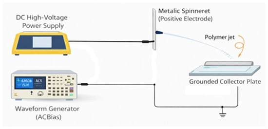
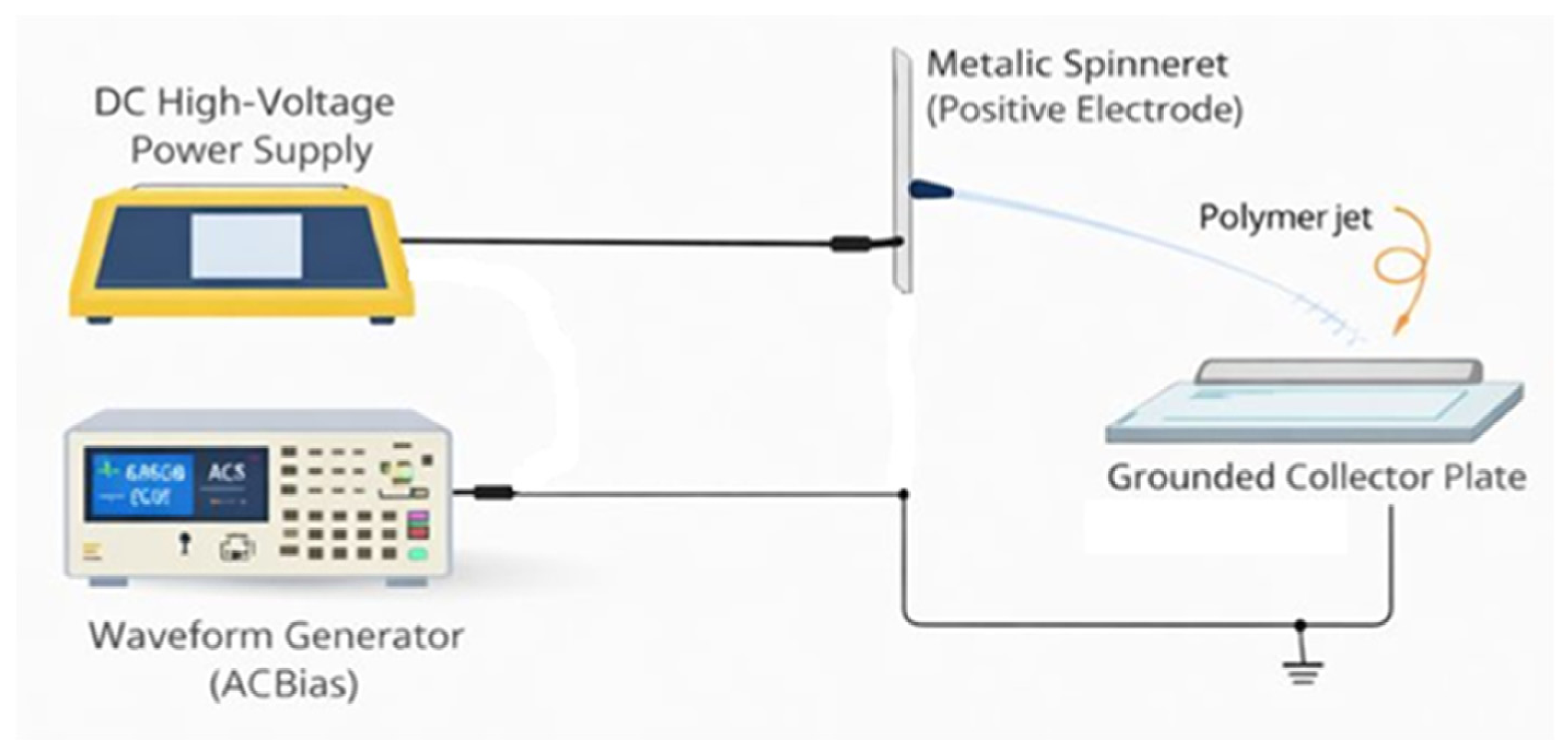
A conventional electrospinning apparatus (Inovenso Starter Kit, Inovenso Ltd. Co., İstanbul, Türkiye), comprising a syringe pump, a stainless-steel needle (21 G, inner diameter ~0.5 mm), and a flat plate collector, was used. The needle was connected to a high-voltage DC supply. For all experiments, a DC voltage of 20 kV was applied to the needle, and a tip-to-collector distance of 20 cm was applied. These base conditions were kept constant to isolate the effect of the AC field. The polymer solution was delivered at a flow rate of 0.5 mL/h, ensuring a steady Taylor cone at the needle tip. PVP solution is electrospun from the needle under the primary DC field, while the collector receives a secondary AC bias (Figure 1). To introduce an AC field, the collector plate (which was normally grounded in the control) was instead connected to the output of a function/arbitrary waveform generator (Multicomp Pro MP750065, Farnell, Leeds, UK) through a power amplifier (a 50 Ω output stage integrated into the generator unit, providing unity gain at the specified amplitude range). The waveform generator can produce standard waveforms (sine, square, ramp, arb) as well as user-defined arbitrary signals, with 14-bit resolution and 125 MS/s sampling rate. In our setup, the generator was configured to output a 1 kHz signal with a peak-to-peak amplitude of 20 V. This low-voltage AC output was fed into a 50 Ω output stage and then to the collector. The collector itself was a 15 × 15 cm aluminum plate, which we covered with aluminum foil to ensure a uniform distribution of the applied field across the surface. The plate was electrically insulated from ground except through the generator. The waveform generator is earth-referenced through its chassis ground terminal. The collector was directly connected to the amplifier output via a coaxial cable without capacitive coupling or electrical isolation. The waveform fidelity was verified at the collector under load using an oscilloscope, and the current delivered at 1 kHz into the predominantly capacitive collector plate was measured to be in the microampere range. The DC high-voltage supply ground and the AC generator ground share a common earth reference through the laboratory mains. A detailed circuit schematic is provided in Figure 1.

Figure 1. A combined experimental setup including the electrospinning under primary DC with a waveform generator as a secondary AC bias.

The combined field experienced by the jet is therefore an oscillating component superimposed on the static DC field between needle and collector. The working hypothesis was that the oscillatory component would perturb the whipping (bending) instability of the charged jet and thereby modify the degree of stretching. The AC amplitude is very low relative to the main DC field (approximately 0.05% of the DC voltage; see Section 1), so it does not appreciably alter the time-averaged electric force and acts, if at all, as a dynamic perturbation.

Four AC waveform conditions were investigated in addition to two controls: (1) sine wave, a sinusoidal voltage of 20 Vp–p at 1 kHz; (2) pulse wave, a 1 kHz square wave (50% duty cycle) of ±10 V amplitude; (3) ramp wave, a sawtooth waveform rising linearly from −10 V to +10 V over each cycle (1 kHz) and dropping back to −10 V sharply at the end of the cycle; and (4) arbitrary/noise wave, a pseudo-random voltage waveform with approximate Gaussian white-noise characteristics bounded between ±10 V. These waveforms allow testing of smooth periodic fields (sine), abrupt switching fields (pulse, which are rich in higher harmonics), asymmetric periodic fields (ramp) and a stochastic field (noise). All waveforms were AC-coupled around 0 V (no DC offset). The generator output was monitored with an oscilloscope to confirm amplitude and waveform fidelity under load. Because the main electrospinning high voltage is supplied by the DC source at the needle, the presence of the AC signal does not appreciably change the time-averaged electric field magnitude between needle and collector, which for 20 kV across a 0.20 m gap is approximately 1 × 10⁵ V m⁻¹ (0.1 MV m⁻¹). The oscillating component (±10 V over the same 0.20 m gap, i.e., ±50 V m⁻¹) is approximately three orders of magnitude smaller than this mean DC field. A “control (connected)” test was also included, in which the function generator was connected to the collector but set to 0 V output, in order to control for the impedance of the generator and the presence of the circuit independently of the oscillation. This was in addition to the standard control with the collector simply grounded. Six conditions were therefore compared: DC only (grounded collector), DC with generator connected at 0 V, and DC with AC sine, pulse, ramp and noise waveforms. Each condition was run three times as independent electrospinning runs.

2.3. SEM Image Recording and Fiber Diameter Analysis

After electrospinning for 10 min, the fibers were characterized morphologically using a Zeiss Ultra Plus field-emission SEM (Zeiss Ultra Plus, Carl Zeiss Microscopy GmbH, Oberkochen, Germany) at an accelerating voltage of 1–2 kV (low-voltage imaging was used to reduce charging on the non-conductive PVP). Before SEM analysis, the samples were sputter-coated with a 5 nm gold layer to enhance conductivity and minimize charging artifacts. For each sample, at least five representative areas were imaged at magnifications between 1000× and 10,000×. From these images, fiber diameters were measured using FIJI/ImageJ (version 1.54r; National Institutes of Health, Bethesda, MD, USA). One hundred fibers were measured per condition, distributed across the three independent runs of that condition (approximately 33–34 fibers per run, taken from several images per run); the sampling scheme and its statistical consequences are set out in Section 2.6. The data were compiled to calculate the mean fiber diameter, the standard deviation, and the minimum and maximum observed diameters for each condition. Any occurrence of bead defects (qualitatively identified as spindle-like thicker sections or spherical beads along fibers) was also noted. We acknowledge that the fiber-diameter measurements were performed manually using FIJI/ImageJ and were not conducted in a blinded fashion; this is noted as a methodological limitation.

2.4. Profilometry (Surface Topography)

To assess the topography of the deposited fiber mats, a contact profilometer (Bruker Dektak XT, Bruker Nano Surfaces Division, Tucson, AZ, USA) was used. This instrument maps the surface height profile along a line scan with sub-micron vertical resolution. For each sample, line scans of approximately 1.0 mm were recorded across the fiber mat in two orthogonal directions (denoted X and Y). From these height profiles, roughness parameters were evaluated in accordance with ISO 4287 [22]. after least-squares removal of the mean line: the arithmetic mean roughness Ra, the root-mean-square roughness Rq, the maximum peak-to-valley height Rt, and the skewness Rsk. Because a single representative X profile and a single representative Y profile were recorded per condition, no inferential statistics were performed on the roughness data; the two orthogonal scans are reported as the spread of the measurement and the values are presented as descriptive rather than statistically compared quantities. All other quantitative data are reported as mean ± standard deviation.

Profilometry measurements were not performed in a blinded fashion, regional uniformity across different areas of the mat was not systematically characterized, and only one profile per direction per condition was acquired; these are noted as limitations. Representative profiles were selected from the central region of each mat.

2.5. Quantitative Fiber Orientation Analysis Theory

Fiber orientation was quantified from the 1000× SEM panels, which were acquired at identical magnification for all six conditions and therefore permit direct comparison; the higher-magnification panels were not used for orientation analysis because they were not acquired at a common magnification across conditions. Two independent estimators were applied to each micrograph. The first is a gradient structure-tensor analysis, in which the local fiber direction is taken as normal to the intensity gradient, and the orientation histogram is weighted by the gradient magnitude, retaining only pixels above the 60th percentile of the gradient magnitude [23,24]. The second is a two-dimensional fast Fourier transform (FFT) analysis, in which the angular distribution of spectral power is integrated over an annular spatial-frequency band (0.02–0.30 cycles per pixel) after application of a Hann window. For both estimators, the degree of alignment is reported as the two-dimensional Herman orientation factor,

S = 2⟨cos²(θ − θ₀)⟩ − 1,

(1)

where θ₀ is the modal orientation and the average is taken over the weighted orientation distribution. S = 1 denotes perfect uniaxial alignment and S = 0 an isotropic (random) fiber mat. Because any finite image of randomly oriented fibers returns a small non-zero S, the isotropic noise floor of the method was established separately for each estimator by applying the identical pipeline to twelve synthetic images of randomly oriented fibers, giving S = 0.062 ± 0.027 (95th percentile S95 = 0.104) for the structure tensor and S = 0.094 ± 0.031 (S95 = 0.141) for the FFT estimator. The pipeline was validated on synthetic fiber images of known orientation, returning S = 1.00 for perfectly aligned fibers, S = 0.81 for a partially aligned population (Gaussian orientation distribution, σ = 20°) and S = 0.11 for randomly oriented fibers. Values of S are compared against the noise floor of the corresponding estimator, and Equation (1) is applied identically to all conditions.

2.6. Statistical Analysis

Each of the six conditions was produced in three independent electrospinning runs. One hundred fiber diameters per condition were measured from SEM images pooled across those three runs (approximately 33–34 fibers per run). The statistical unit used in the inferential analysis is therefore the individual fiber, not the independent run. This is stated explicitly because it constitutes pseudoreplication with respect to the experimental unit: the 100 diameters within a condition are not fully independent, since fibers from the same run share the run-level sources of variation (solution batch, ambient humidity, needle condition). The consequence is that the effective sample size is smaller than n = 100 and the reported p-values are anti-conservative. The values below should accordingly be read as a descriptive comparison of pooled fiber-level diameter distributions rather than as a test of the run-level treatment effect, and the significance thresholds should not be interpreted as establishing a reproducible between-run difference. A properly powered test of the treatment effect would require the run mean as the statistical unit (n = 3 per condition), or a linear mixed-effects model with run as a random intercept; neither is well determined at three runs per condition, and this is identified as a limitation of the present design in Section 5. One-way analysis of variance (ANOVA) followed by Tukey’s honestly significant difference (HSD) post-hoc test was applied to the pooled fiber-level measurements, with significance set at p < 0.05.

3. Results

3.1. Fiber Morphology Under DC vs. AC Fields

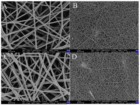
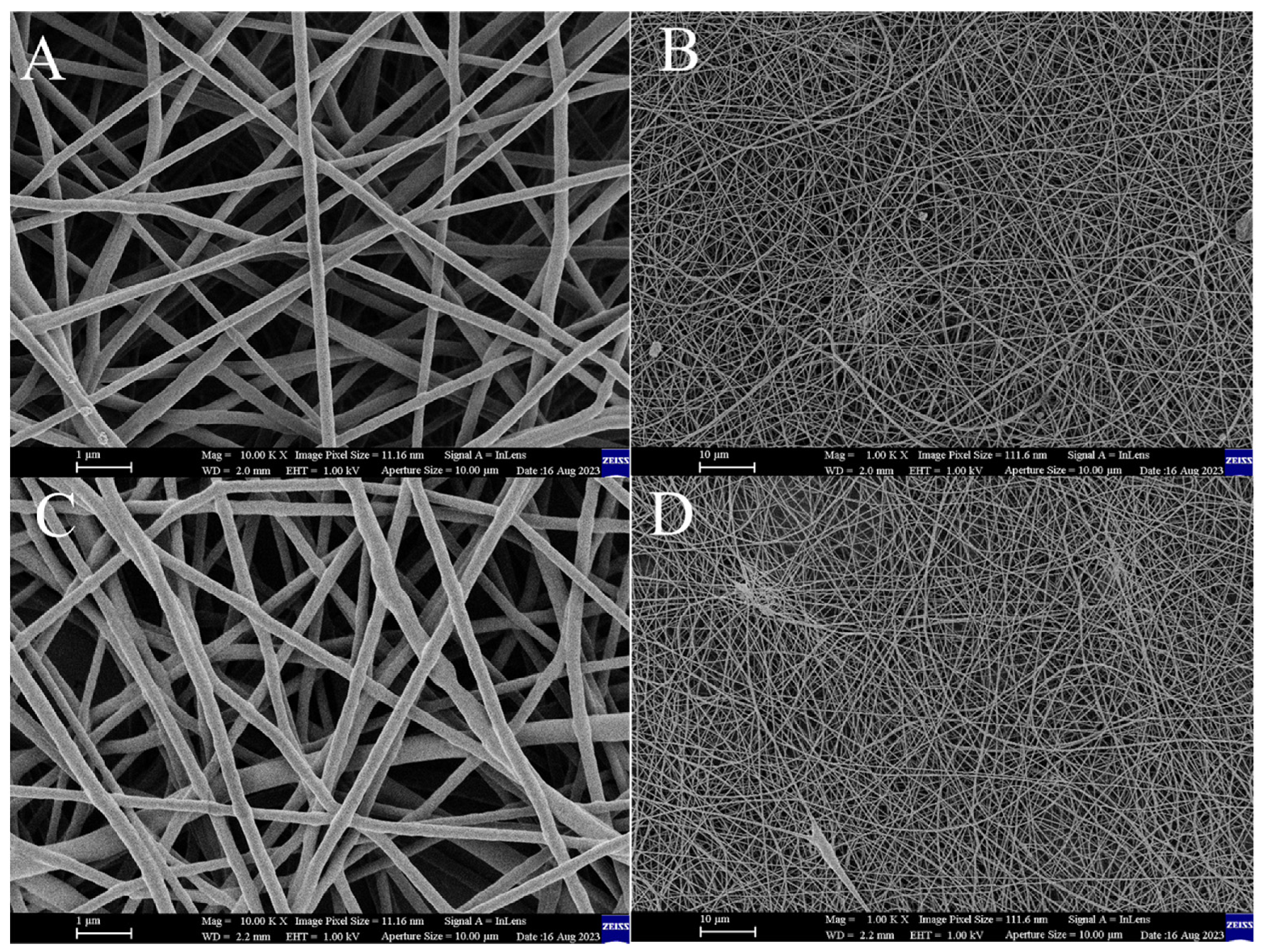
The baseline PVP electrospinning (standard DC field, grounded collector) produced the expected randomly oriented nanofiber mat. SEM images of the control sample (Figure 2A,B) reveal fibers with an average diameter of 215 nm and occasional beads or thick segments.

Figure 2. SEM images of electrospun PVP nanofibers obtained under baseline DC electrospinning conditions: (A) control (grounded collector) at 10,000× magnification, (B) control at 1000× magnification, (C) control-connected condition (collector connected to the function generator with 0 V output) at 10,000× magnification, and (D) control-connected at 1000× magnification. Scale bars: 1 µm (A,C) and 10 µm (B,D). Panels (A,C) are shown at the same magnification to facilitate direct comparison.

The diameter distribution for the DC control was relatively broad (standard deviation ~47 nm), indicating appreciable variability in fiber thickness. This is common in electrospinning, where minor fluctuations in the jet can cause some fibers to be thinner than others. A small number of bead defects were observed in the control images, appearing as spindle-like enlargements along the fibers. When the function generator was attached with 0 V output (the “control-connected” case, Figure 2C,D), the fibers had a larger mean diameter (~237 nm) and a broader distribution (standard deviation ~52 nm) than the plain control. This difference is attributed to the collector not being a perfect ground in this configuration: the 50 Ω output impedance of the generator to ground alters the electric boundary condition, leaving the collector at a floating potential close to 0 V, which would slightly reduce the effective field and hence the stretching force on the jet. This shows that the electrical environment of the collector, independently of any oscillation, can affect fiber morphology—a point developed further in Section 3.2 and Section 4.1. All of the active AC waveform cases described next should therefore be compared against both the connected and grounded controls.

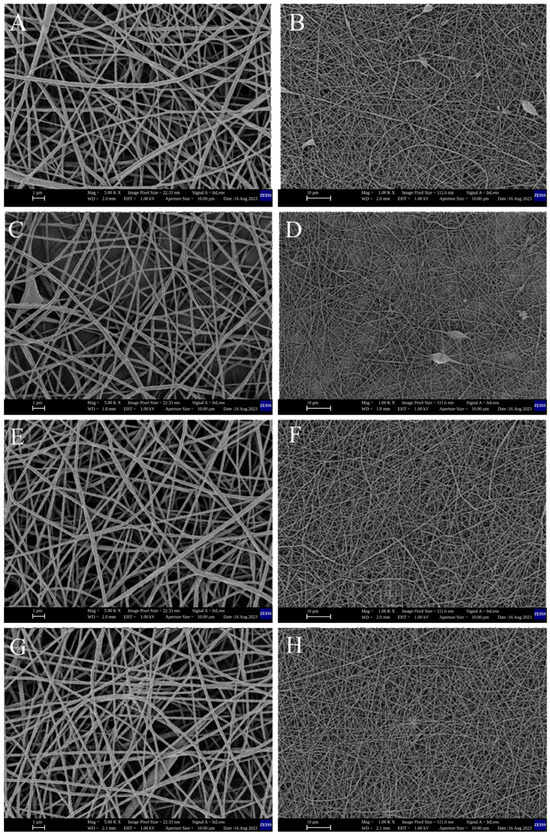
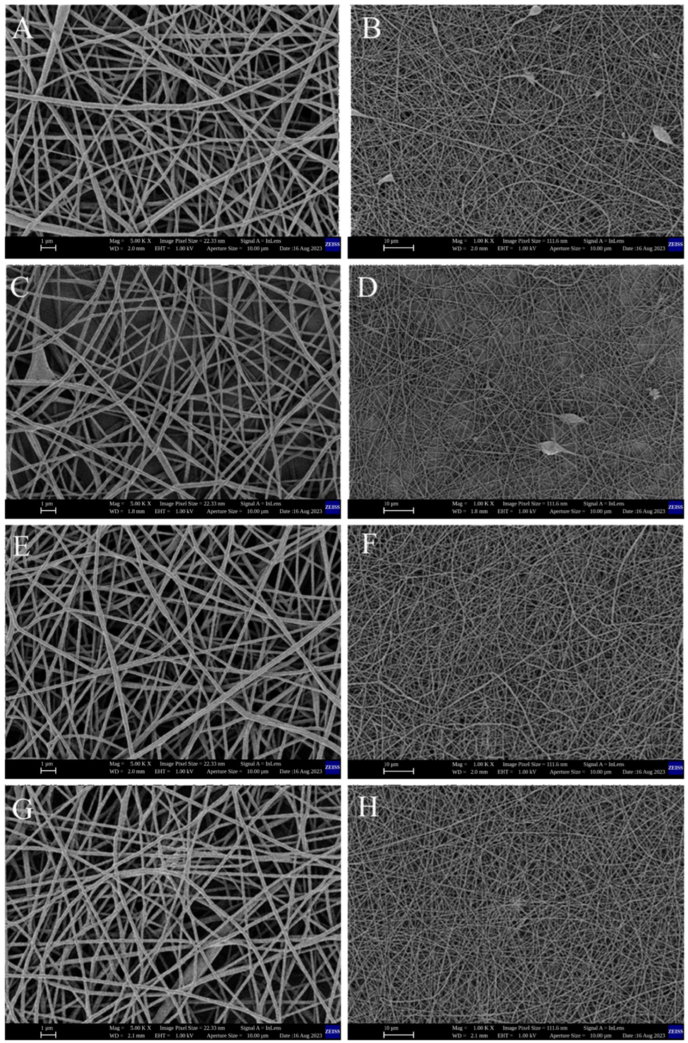
With a 1 kHz sinusoidal 20 Vp–p applied to the collector, a noticeable change in the fiber deposition behavior was observed. During electrospinning, the jet visually appeared to whip more vigorously in the presence of the AC field, as anticipated. The SEM images (Figure 3A,B) for the sine-wave case show fibers that are, on average, 224 nm in diameter, slightly thinner than the control-connected fibers. The diameter spread (std ~64 nm) was somewhat higher for sine-wave fibers, and a few bead defects were still present. The increase in variability could be due to the continuous sinusoidal modulation causing a mix of stretching and relaxing phases each cycle—while the field is in one polarity, the jet is pulled slightly stronger, and half a cycle later, slightly weaker (since the needle remains positively charged at 20 kV, the collector’s oscillation from 0 to ±10 V effectively modulates the field strength by ±0.05%). If the frequency is high enough (1 kHz) that the jet cannot fully respond to each polarity switch, the result might be a quasi-periodic fluctuation in the fiber diameter along its length—possibly explaining the higher variability.

Figure 3. SEM micrographs of PVP nanofibers electrospun with a 20 Vp–p, 1 kHz AC signal applied to the collector: sine (A,B), square/pulse (C,D), ramp (E,F) and arbitrary noise (G,H) waveforms. Panels (A,C,E,G) were acquired at 5000× magnification (scale bar 1 µm); panels (B,D,F,H) at 1000× magnification (scale bar 10 µm). Note that the high-magnification panels here (5000×) are not at the same magnification as the high-magnification panels of Figure 2 (10,000×); cross-figure comparison should therefore use the 1000× panels, which are common to both figures.

Fiber orientation under the sine waveform was assessed quantitatively (Section 3.3) rather than by visual impression. The fibers in Figure 3A,B form a nonwoven mat with no orientation preference detectable above the noise floor of the orientation analysis.

The square (pulse) waveform produced the broadest diameter distribution. Here the collector potential switched between +10 V and −10 V every 0.5 ms. The SEM images (Figure 3C,D) show a mean fiber diameter of approximately 212.6 nm, close to that of the grounded DC control, but with the widest distribution of all conditions (standard deviation ~70 nm). Both thin fibers and thicker spindle-like sections are present, and Figure 3C,D show a mixture of fine fibers and occasional beaded segments. This outcome is qualitatively consistent with the report of Sivan et al. [15] for square-wave AC electrospinning of polycaprolactone, in which abrupt field transitions were associated with broader, multimodal diameter distributions; we note that their observation was obtained at high AC voltage and at 30 Hz, so the comparison is suggestive rather than direct. The pulsed waveform did not produce fiber alignment: quantitative orientation analysis (Section 3.3) returns among the lowest orientation factors of all six conditions for this waveform, at or below the noise floor of both estimators. The apparent “bundles” visible in Figure 3C,D are local fiber crossings and overlapping segments and are not distinguishable from the arrangement seen in the DC control.

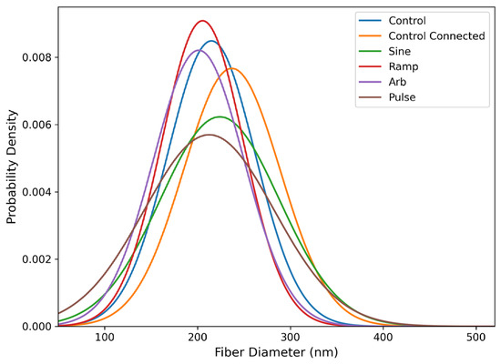
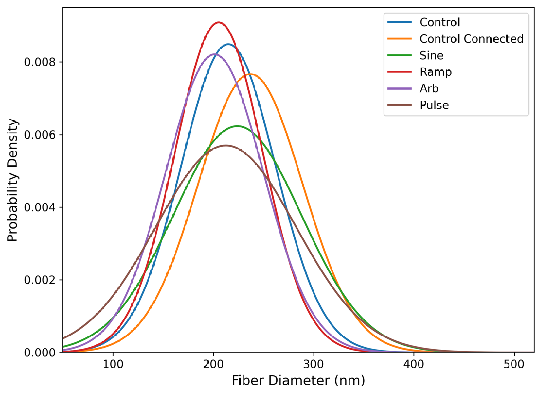
The ramp (sawtooth) waveform produced the most uniform fiber diameters. SEM images (Figure 3E,F) show fibers that are thinner and more uniform than in the other conditions. The mean diameter was approximately 205.5 nm and the standard deviation ~43.9 nm, the lowest of all samples. The diameter histogram (Figure 4) for the ramp condition is correspondingly narrow, and few bead defects are visible in Figure 3E,F. One possible interpretation is that the linear rise and abrupt reset of the ramp impose a predominantly unidirectional stretching over most of the cycle, followed by a rapid reset; this is offered as a hypothesis only, since no measurement of jet trajectory or jet current was made and the alternative explanation that the difference reflects run-to-run variability cannot be excluded at three runs per condition. The ramp waveform did not produce fiber alignment (Section 3.3), and it did not produce the flattest mat: its surface roughness was the highest of the four AC conditions (Section 3.2).

Figure 4. Histogram of fiber-diameter distributions. X-axis: Fiber Diameter (nm); Y-axis: Probability Density.

Under the arbitrary noise waveform, the SEM micrographs (Figure 3G,H) show fibers with a mean diameter of approximately 201.3 nm—the smallest mean of all conditions—and a standard deviation of approximately 48.6 nm, comparable to the grounded control. The noise waveform therefore achieved a reduction in mean diameter without an increase in variability. A random waveform introduces a broad spectrum of frequencies, some of which may coincide with the growth rates of the jet instability; this remains a conjecture, as no spectral measurement of the jet was performed. Fibers under the noise waveform are generally bead-free, although less uniform in diameter than in the ramp condition, and show no preferential orientation (Section 3.3).

Figure 4 presents histograms of the fiber-diameter distributions for all conditions, allowing the uniformity of each distribution to be compared directly. The corresponding summary statistics—mean, standard deviation, minimum and maximum diameter, number of independent runs and n, are given in Table 1, and the inferential statistics in.

Table 1. Summary of fiber diameter statistics for all experimental conditions.

Condition	Mean (nm)	SD (nm)	Min (nm)	Max (nm)	Runs	n
Control (grounded)	215	47	171	339	3	100
Control (connected)	237	52	166	442	3	100
Sine AC	224	64	145	405	3	100
Pulse AC	212.6	70.0	117	460	3	100
Ramp AC	205.5	43.9	135	344	3	100
Noise AC	201.3	48.6	132	400	3	100

Note: n = 100 pooled fiber-diameter measurements per condition, obtained from SEM images across three independent electrospinning runs (≈33–34 fibers per run). The statistical unit is the individual fiber; see Section 2.6 for the pseudoreplication caveat. Statistical comparison: one-way ANOVA with Tukey HSD post-hoc test. Ramp, noise and pulse conditions differ significantly from the connected control; no condition differs significantly from the grounded control. Full post-hoc statistics.

The grounded control fibers had a mean diameter of approximately 215 nm (min ~171 nm, max ~339 nm). The connected control had a higher mean of approximately 237 nm and a wider range (min ~166 nm, max ~442 nm). Under sine AC the mean was ~224 nm (min ~145 nm, max ~405 nm); ramp AC gave a mean of ~205.5 nm (min ~135 nm, max ~344 nm); noise AC ~201.3 nm (min ~132 nm, max ~400 nm); and pulse AC ~212.6 nm (min ~117 nm, max ~460 nm). One-way ANOVA over the six conditions was significant (F(5.594) = 5.56, p = 5.1 × 10⁻⁵), but the effect size was small: one of the conditions accounted for 4.5% of the total variance in fiber diameter (η² = 0.045, ω² = 0.037), with a pooled within-condition standard deviation of 55.1 nm. The choice of comparator is decisive for the interpretation and is therefore stated explicitly. Against the connected control, the ramp (−31.5 nm, p = 0.0008), noise (−35.7 nm, p = 0.0001) and pulse (−24.4 nm, p = 0.022) waveforms all produced significantly finer fibers. Against the grounded control, however, no AC condition reached significance (ramp p = 0.83; noise p = 0.49; pulse p > 0.99; sine p = 0.86), and the difference between the two controls themselves was itself borderline (p = 0.055). The only other significant pairwise difference was sine versus noise (22.7 nm, p = 0.043). The corrected statement is therefore that the ramp and noise waveforms produce a significant reduction in fiber diameter relative to the impedance-matched connected control, but not relative to a conventional grounded collector; the reduction relative to the connected control is approximately 13–15%, whereas relative to the grounded control it is approximately 4–6% and is not statistically supported. These p-values are subject to the pseudoreplication caveat set out in Section 2.6.

3.2. Deposition Pattern and Surface Topography

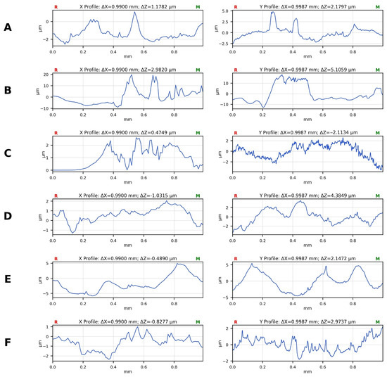
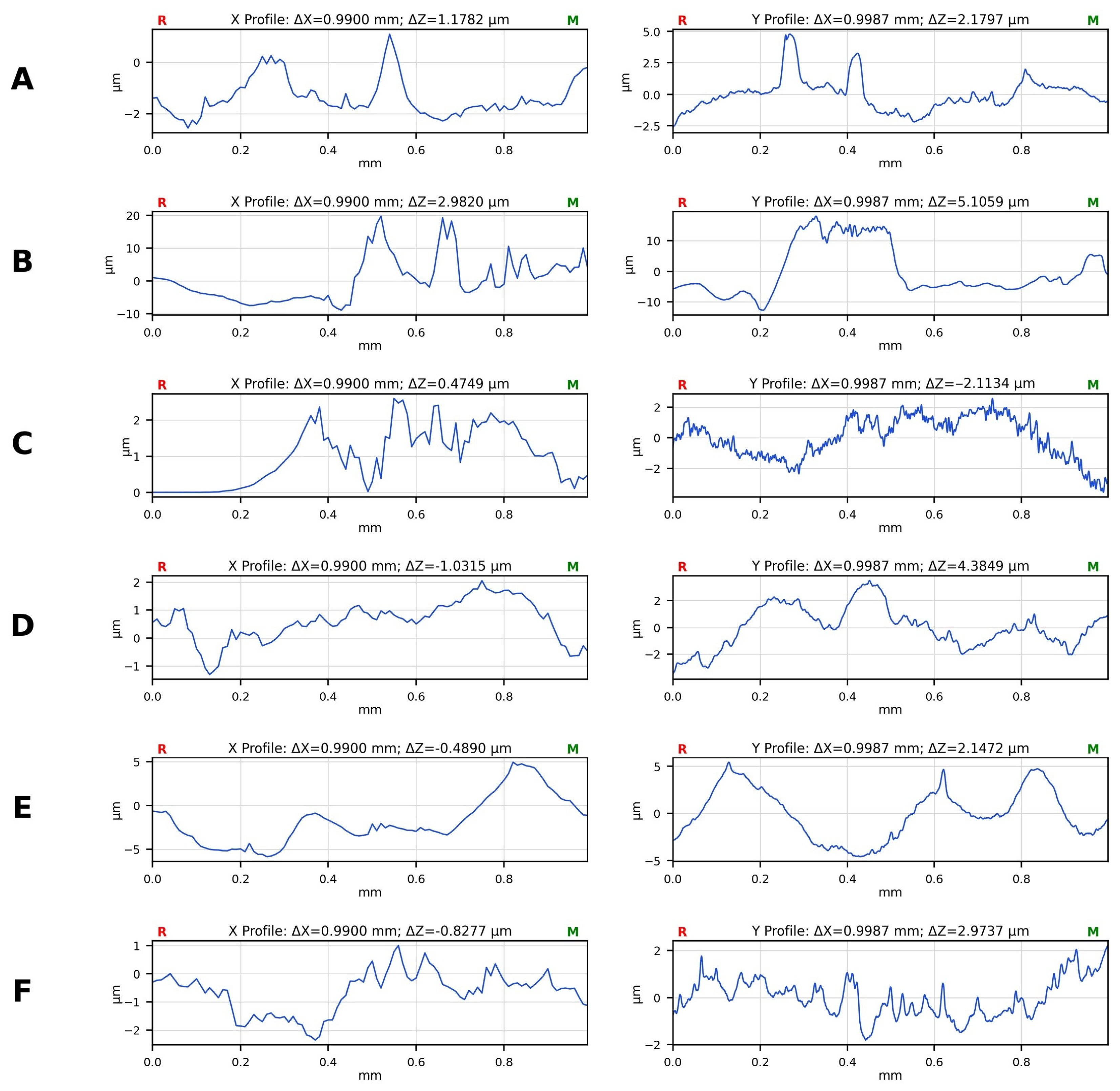
Surface topography was quantified from the profilometry traces of Figure 5 using the roughness parameters defined in Section 2.4; the results are collected in Table 2. Two findings emerge. First, the connected control is a clear outlier: its mat is far rougher than every other condition (Ra = 5.73 µm, Rt = 29.0 µm, against Ra = 0.61–1.95 µm and Rt = 3.6–8.6 µm for all other conditions). This is consistent with the collector being held at a floating potential through the 50 Ω output stage of the generator rather than at true ground, which alters the electrical boundary condition at the collector and appears to promote uneven deposition. Second, among the AC waveforms the noise condition produced the smoothest mat (Ra = 0.61 µm, Rt = 3.56 µm), marginally smoother than the grounded DC control (Ra = 0.74 µm, Rt = 5.47 µm), while the sine (Ra = 0.83 µm) and pulse (Ra = 0.85 µm) conditions were indistinguishable from the grounded control at this level of sampling. The ramp waveform produced the roughest mat of the four AC conditions (Ra = 1.95 µm, Rt = 8.61 µm), approximately 2.6 times rougher than the grounded control. The ramp waveform therefore combines the narrowest fiber-diameter distribution with the roughest mat surface, indicating that fiber-scale uniformity and mat-scale uniformity are not equivalent measures and do not necessarily improve together. Because only one profile per direction per condition was acquired, these differences are descriptive; with n = 1 per scan direction the roughness values cannot be compared inferentially, and the smaller differences between the grounded control and the sine, pulse and noise conditions should not be regarded as established.

Figure 5. Representative contact-profilometry height profiles of the deposited fiber mats for (A) grounded control, (B) connected control, (C) sine, (D) pulse, (E) ramp and (F) noise waveform conditions. For each condition the left panel is the X-direction scan and the right panel the Y-direction scan; the scan length is approximately 1.0 mm in both directions. Note the differing vertical scales between panels. Roughness parameters derived from these profiles are given in Table 2.

Table 2. Surface roughness parameters derived from the profilometry height profiles of Figure 5 (ISO 4287, after least-squares form removal). X and Y denote the two orthogonal scan directions; mean values are the average of the two. Rsk is the profile skewness, averaged over the two directions. A single profile per direction per condition was acquired, so no inferential statistics are reported.

Condition	Ra, X (µm)	Ra, Y (µm)	Ra Mean (µm)	Rq Mean (µm)	Rt Mean (µm)	Rsk Mean
Control (grounded)	0.55	0.93	0.74	1.01	5.5	+1.20
Control (connected)	4.38	7.07	5.73	6.98	29.0	+1.04
Sine AC	0.53	1.12	0.83	0.99	4.4	−0.16
Pulse AC	0.49	1.22	0.85	1.09	4.8	−0.40
Ramp AC	1.64	2.25	1.95	2.33	8.6	+0.44
Noise AC	0.57	0.65	0.61	0.74	3.6	−0.01

Figure 4 compares the fiber-diameter distributions across all conditions. The ramp and noise waveforms shift the distribution towards finer fibers relative to the connected control, and the ramp waveform gives the narrowest distribution; the sine and pulse waveforms do not reduce the mean diameter, and the pulse waveform increases the variance. These differences are small in absolute terms and are not significant against the grounded control (Table 3).

Table 3. One-way ANOVA for fiber diameter across the six conditions (pooled fiber-level measurements, n = 100 per condition).

Source	SS	df	MS	F	p	Effect Size
Between conditions	84,384	5	16,877	5.56	5.1 × 10−5	η2 = 0.045
Within conditions	1,801,619	594	3033	—	—	ω2 = 0.037
Total	1,886,003	599	—	—	—	pooled SD = 55.1 nm

Figure 5 shows representative surface height profiles of nanofiber mats produced under the different electrical excitation modes. The connected control (Figure 5B) exhibits pronounced height excursions of up to approximately 30 µm peak-to-valley. The DC control (Figure 5A) and the sine, pulse and noise AC conditions (Figure 5C,D,F) all lie within a comparable range of a few micrometres, while the ramp condition (Figure 5E) shows larger, longer-wavelength undulations. Quantitative values are given in Table 2.

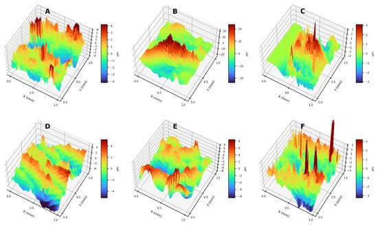
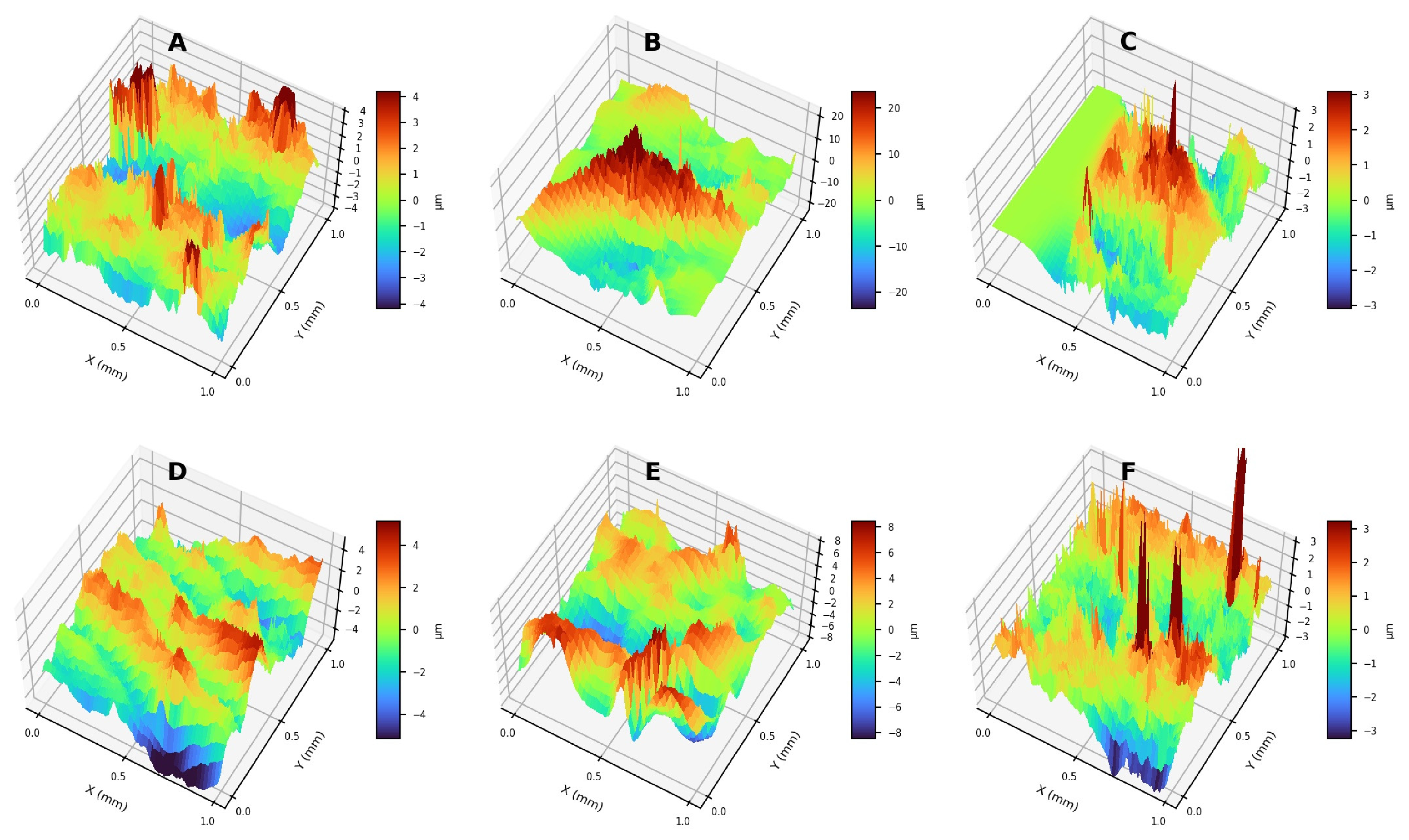
Figure 6 presents three-dimensional surface height maps reconstructed from the profilometry measurements, providing a spatial view of the same data summarized in Table 2. The connected control (Figure 6B) again stands out, with a peak-to-valley height approximately 3.4 times that of the next roughest condition and more than five times that of the grounded control. The ramp condition (Figure 6E) shows the largest height excursions of the four AC waveforms and the sine and noise conditions (Figure 6C,F) the smallest. These maps are presented as qualitative support for the numerical parameters in Table 2; because a single map was acquired per condition, they are not used to draw inferential conclusions about fiber packing.

Figure 6. Three-dimensional surface height maps reconstructed from profilometry for (A) grounded control, (B) connected control, (C) sine, (D) pulse, (E) ramp and (F) noise waveform conditions. Note that the vertical colour scale differs between panels; the connected control (B) spans approximately ±20 µm whereas all other conditions span a few micrometres.

Full ANOVA and Tukey HSD statistics are given in Table 3 and Table 4.

Table 4. Tukey HSD post-hoc pairwise comparisons of mean fiber diameter. “Grounded” and “connected” denote the two control conditions. Positive differences indicate that the first condition has the larger mean diameter.

Comparison	Difference (nm)	q	p (Adjusted)	95% CI (nm)	Significant
Grounded vs. Connected	−22.0	3.99	0.0550	[−44.3, 0.3]	no
Grounded vs. Sine	−9.0	1.63	0.8576	[−31.3, 13.3]	no
Grounded vs. Pulse	+2.4	0.44	0.9996	[−19.9, 24.7]	no
Grounded vs. Ramp	+9.5	1.72	0.8272	[−12.8, 31.8]	no
Grounded vs. Noise	+13.7	2.49	0.4933	[−8.6, 36.0]	no
Connected vs. Sine	+13.0	2.36	0.5528	[−9.3, 35.3]	no
Connected vs. Pulse	+24.4	4.43	0.0223	[2.1, 46.7]	yes
Connected vs. Ramp	+31.5	5.72	0.0008	[9.2, 53.8]	yes
Connected vs. Noise	+35.7	6.48	0.0001	[13.4, 58.0]	yes
Sine vs. Pulse	+11.4	2.07	0.6876	[−10.9, 33.7]	no
Sine vs. Ramp	+18.5	3.36	0.1666	[−3.8, 40.8]	no
Sine vs. Noise	+22.7	4.12	0.0428	[0.4, 45.0]	yes
Pulse vs. Ramp	+7.1	1.29	0.9435	[−15.2, 29.4]	no
Pulse vs. Noise	+11.3	2.05	0.6957	[−11.0, 33.6]	no
Ramp vs. Noise	+4.2	0.76	0.9945	[−18.1, 26.5]	no

3.3. Quantitative Fiber Orientation Analysis

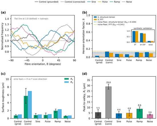
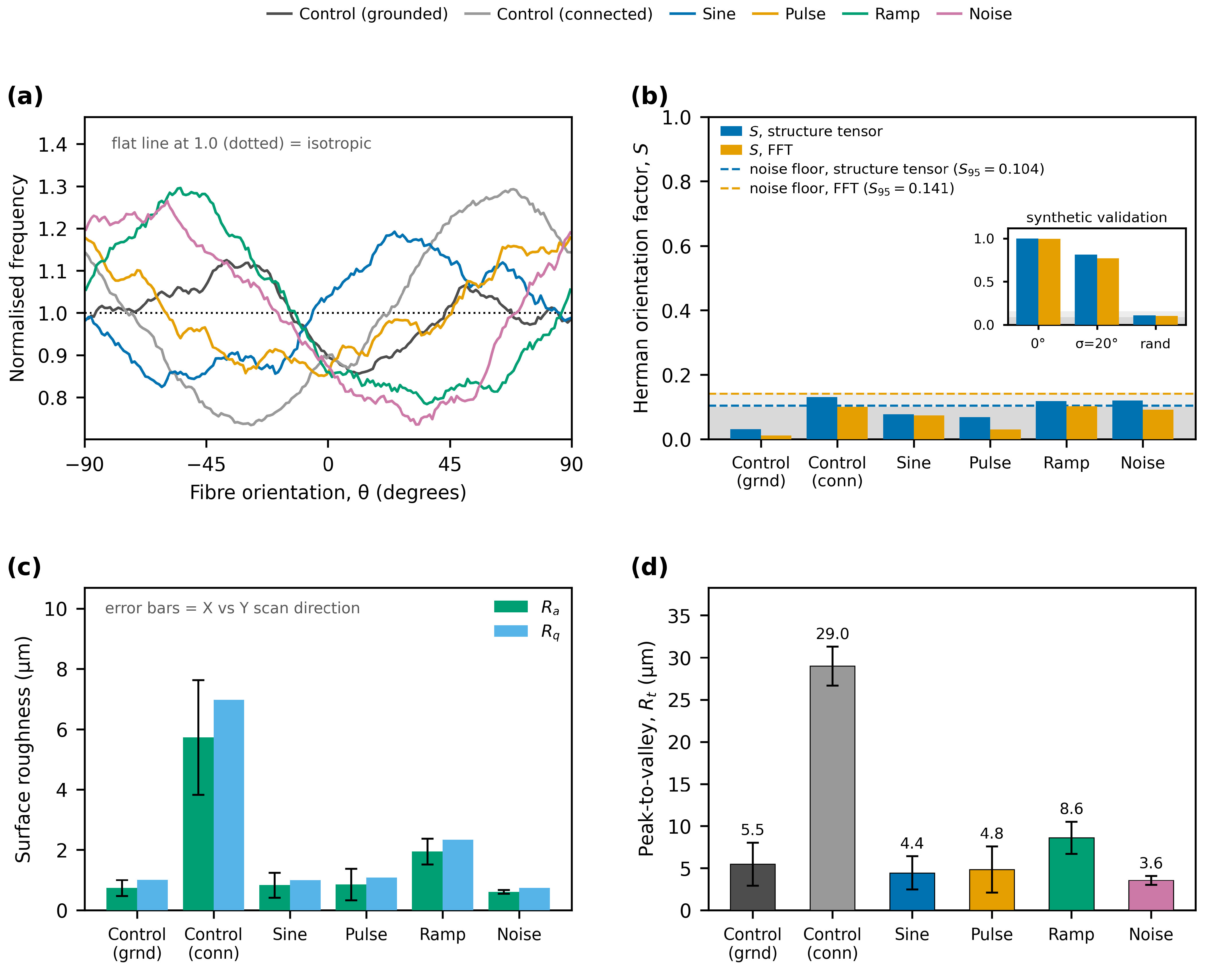
Fiber orientation was quantified for all six conditions using the two independent estimators described in Section 2.5, applied to the 1000× SEM panels. The results are shown in Figure 7 and summarized in Table 5. The Herman orientation factor does not exceed S = 0.13 for any condition by either estimator: structure-tensor values range from 0.031 (grounded control) to 0.130 (connected control), and FFT values from 0.012 to 0.103. For comparison, the same pipeline returns S = 1.00 for perfectly aligned synthetic fibers and S = 0.81 for a partially aligned population with a 20° orientation spread, so every measured value is below one-sixth of the partially aligned benchmark.

Figure 7. Quantitative orientation and surface-roughness analysis. (a) Gradient-weighted orientation distributions obtained by structure-tensor analysis of the 1000× SEM panels, normalized so that an isotropic mat gives a flat line at unity. (b) Two-dimensional Herman orientation factor S for each condition obtained by structure-tensor and FFT estimators; the shaded band is the isotropic noise floor of the method (95th percentile of twelve randomly oriented synthetic images) and the inset shows validation of the pipeline on synthetic fiber images with known orientation (perfectly aligned, partially aligned with σ = 20°, and random). (c) Arithmetic mean roughness Ra and root-mean-square roughness Rq from the profiles of Figure 5; error bars indicate the spread between the X and Y scan directions. (d) Maximum peak-to-valley height Rt for each condition.

Table 5. Quantitative fiber orientation results. S is the two-dimensional Herman orientation factor (S = 0 isotropic, S = 1 perfectly aligned), computed by two independent estimators on the 1000× SEM panels. Isotropic noise floors determined on randomly oriented synthetic images are S = 0.062 ± 0.027 (S95 = 0.104) for the structure tensor and S = 0.094 ± 0.031 (S95 = 0.141) for the FFT estimator; each value is compared against the floor of its own estimator.

Condition	S (Structure Tensor)	S (FFT)	Exceeds Isotropic Noise Floor?
Control (grounded)	0.031	0.012	no
Control (connected)	0.130	0.101	no
Sine AC	0.078	0.074	no
Pulse AC	0.069	0.031	no
Ramp AC	0.118	0.103	no
Noise AC	0.120	0.092	no
Synthetic, perfectly aligned (0°)	1.000	0.996	yes (validation)
Synthetic, partially aligned (σ = 20°)	0.814	0.771	yes (validation)
Synthetic, random	0.108	0.103	no (validation)

Figure 7 shows the full quantitative orientation and surface-roughness analysis.

The comparison against the isotropic noise floor requires care, because the two estimators have different floors: S95 = 0.104 for the structure tensor and S95 = 0.141 for the FFT (Section 2.5). By the FFT estimator no condition exceeds its floor. By the structure-tensor estimator three conditions marginally exceed it, the connected control (0.130), the noise waveform (0.120) and the ramp waveform (0.118), and for the ramp and noise conditions the two estimators return preferred directions that agree to within 7–9°. We therefore do not claim that these mats are perfectly isotropic: a weak residual anisotropy of order S ≈ 0.12 cannot be excluded for those three conditions. What the data do establish is that such anisotropy as exists is not attributable to the AC field. The largest orientation factor of all six conditions belongs to the connected control, which received no oscillating signal at all; the grounded control returns the smallest value (0.031); and the pulsed waveform, which the original analysis identified as the most strongly aligned condition, falls at or below both noise floors (S = 0.069 by structure tensor, S = 0.031 by FFT). There is no ordering of the orientation factors that corresponds to the presence, absence or shape of the applied waveform.

The alignment claims made previously are therefore withdrawn. No AC waveform produced fiber alignment attributable to the applied field, and any residual anisotropy is an order of magnitude weaker than the partially aligned reference case. The features previously interpreted as aligned bundles are local fiber crossings and overlapping segments that are not distinguishable from the arrangement seen in the DC control. The analysis is limited to the field of view of one representative micrograph per condition; a mat-scale orientation measurement (for example, small-angle X-ray scattering, or a tiled montage over several square millimetres with replicate fields per condition) would be required to characterise the weak residual anisotropy properly and to exclude alignment on length scales larger than the imaged field.

4. Discussion

4.1. Mechanistic Interpretation

The differences in fiber diameter observed with certain AC waveforms may be considered in terms of the electrohydrodynamic forces acting on the jet, but it should be stated at the outset that the following account is interpretive. No measurement of jet trajectory, jet current, deposited charge or field distribution was performed in this study, and none of the mechanisms below are established by the present data. In a DC field the charged jet accelerates towards the collector and undergoes the whipping instability, driven principally by self-repulsion of charge within the jet and by ambient perturbation. When an AC component is superimposed, the field at the collector oscillates, so the force on a given jet segment varies periodically. At 1 kHz this variation is fast relative to the millisecond-scale flight time. A plausible consequence is that the jet experiences a rapidly varying tensile force, so that no single segment experiences a sustained constant tension; this could in principle yield more uniform thinning and would be most pronounced for the ramp waveform, where the applied change is monotonic over most of the cycle. This is consistent with the observed narrowing of the ramp diameter distribution, but consistency is not demonstration: the effect size is small (η² = 0.045), the difference is not significant against the grounded control, and a run-to-run explanation cannot be excluded at three runs per condition. It has also been suggested in the AC electrospinning literature that field oscillation dissipates charge from deposited fibers and thereby reduces electrostatic repulsion between them [16]. Whether such an effect operates here is doubtful on quantitative grounds: the oscillating component is approximately three orders of magnitude smaller than the DC field, the collector is a good conductor covered with aluminium foil, and no measurement of surface charge or of mat current was made. Charge neutralization is therefore not advanced here as an explanation of the present results and is retained only as one hypothesis among several that future work could test directly by measuring jet current and deposited charge. The observation that the connected control produced both the thickest fibers and by far the roughest mat is the clearest electrical effect in the dataset, and it is attributable to the altered boundary condition at the collector rather than to the oscillation, since no oscillation was applied in that condition. Comparable sensitivity of deposition uniformity to the collector electrical configuration has been reported for auxiliary-electrode geometries [20].

With respect to fiber alignment, the quantitative analysis in Section 3.3 shows no measurable preferential orientation under any waveform. This is not unexpected on physical grounds. A single flat collector held at a spatially uniform potential provides no lateral field gradient and therefore no preferred axis along which the jet could be swept; alignment in AC-assisted electrospinning has previously been achieved with a DC-biased AC field applied across a gap between two electrodes, which does define such an axis [17]. In addition, the jet flight time was not measured here, so it is not established whether the jet responds to individual 1 ms cycles or integrates over many of them; neither case would produce a directional response in this geometry. Both considerations suggest that alignment with this configuration requires a lower frequency and a collector geometry that defines a preferred direction, for example, a gap or parallel-electrode collector. This is proposed as a direction for future work and is not demonstrated here.

The frequency used here (1 kHz) corresponds to an oscillation period of 1 ms, which is comparable to the estimated flight time of the jet, so the jet is unlikely to respond to individual cycles. Lower frequencies (for example, 10–100 Hz) would allow the jet to track the field oscillation more closely. All mechanisms proposed in this section require experimental verification through high-speed jet imaging, in situ jet-current and deposited-charge measurement, and electric-field modelling of the needle–collector geometry; none of these were performed in the present study.

4.2. Safety and Practicality

One practical advantage of the configuration demonstrated here is its simplicity and safety. The AC voltage used (20 V peak-to-peak) is very low, and the method uses a standard function generator rather than a dedicated high-voltage AC supply. The alternating power available at the generator output is approximately 1 W into a matched 50 Ω load (20 V peak-to-peak corresponds to 7.07 V rms); the collector, however, presents a predominantly capacitive load rather than a matched resistive one, and the current measured at the collector was in the microampere range, corresponding to a delivered power of the order of tens of microwatts. The energy cost of the process is therefore essentially unchanged from the base DC case. At 20 V the AC component is far below the threshold for corona discharge or arcing in air, and no corona was observed; this contrasts with high-voltage AC electrospinning systems, in which corona is deliberately generated to initiate multiple jets. The approach is therefore a retrofittable addition to existing electrospinning equipment. It should be emphasized that this is a statement about the practicality of the hardware, not about the magnitude of the benefit obtained, which on the present evidence is modest and is demonstrated only for one polymer at one amplitude and one frequency.

4.3. Potential Future Directions

The following applications are potential future directions rather than demonstrated benefits of the present work; this study establishes only that waveform shape produces a small, measurable change in the fiber-diameter distribution and mat roughness of one PVP system. If the modest improvement in diameter uniformity observed for the ramp waveform were confirmed across polymer systems and at run level, it could be relevant to filtration membranes, where uniform fiber diameter contributes to consistent pore size. Applications that require aligned fibers, including nerve, muscle and tendon scaffolds and anisotropic sensor architectures, are not addressed by this work: the quantitative orientation analysis reported in Section 3.3 shows that the present configuration does not produce aligned fibers. Whether a lower-frequency signal combined with a gap or parallel-electrode collector could produce alignment at low voltage remains an open question and is, in our view, the most direct extension of this work.

In summary, this study shows that the shape of a low-voltage AC signal applied to the collector produces a small but measurable change in the fiber-diameter distribution of electrospun PVP and no measurable change in fiber orientation. The effect on diameter is significant relative to an impedance-matched connected control but not relative to a conventional grounded collector and accounts for approximately 4.5% of the total variance in fiber diameter. These improvements were obtained without additional high-voltage hardware or any changes to the solution or the primary process parameters. The concept could be extended by exploring different frequencies and amplitudes and by tailoring arbitrary waveforms; the present data do not indicate which, if any, of these directions will prove productive.

The scope of this study is deliberately narrow, and its limitations should be weighed against the conclusions drawn. A single AC amplitude (20 V peak-to-peak), a single frequency (1 kHz), and a single-polymer/solvent system (PVP in 3:1 ethanol/water) were examined, so neither the optimality of these parameters nor the generality of the observed trends across polymer systems can be assessed from these data. Solvent properties such as dielectric constant, conductivity, and evaporation rate strongly influence jet charge dynamics, and testing a non-aqueous system (for example, polycaprolactone in chloroform/DMF) would be required before any claim of general applicability. A systematic amplitude series (for example, 5, 10, 20, and 50 V) and a frequency series spanning 10 Hz to 10 kHz would be needed to establish dose–response behavior and to test whether the absence of alignment at 1 kHz reflects the jet’s inability to track the field. Finally, three independent runs per condition, with statistics computed on pooled fiber-level measurements, do not support strong claims of reproducibility; a design with more runs and run-level statistics would be required.

5. Conclusions

The effect of low-amplitude AC electric fields on nanofiber morphology was evaluated by applying a 20 V peak-to-peak, 1 kHz AC voltage with four different waveforms to the collector during PVP electrospinning, against both grounded and an impedance-matched connected control. Waveform shape produced a small but statistically detectable effect on the fiber-diameter distribution and no detectable effect on fiber orientation.

One-way ANOVA across the six conditions was significant (F(5.594) = 5.56, p = 5.1 × 10⁻⁵) with a small effect size (η² = 0.045). Relative to the connected control, the ramp, noise and pulse waveforms produced significantly finer fibers (13%, 15% and 10% reductions in mean diameter; Tukey HSD p = 0.0008, 0.0001 and 0.022). Relative to a conventional grounded collector, no waveform produced a statistically significant change in mean diameter. The ramp waveform gave the narrowest diameter distribution (205.5 ± 43.9 nm) and the noise waveform gave the smallest mean diameter (201.3 ± 48.6 nm). These comparisons rest on pooled fiber-level measurements and are subject to the pseudoreplication caveat set out in Section 2.6.

Quantitative orientation analysis by two independent estimators returned Herman orientation factors of S ≤ 0.13 for all six conditions, against S = 1.00 for perfectly aligned and S = 0.81 for partially aligned synthetic fibers. No condition exceeded the FFT noise floor; three marginally exceeded the structure-tensor floor, but the largest value belonged to the connected control, which received no oscillating signal, and the pulsed waveform fell at or below both floors. A weak residual anisotropy of order S ≈ 0.12 cannot be excluded in some samples, but it does not track the presence or shape of the applied waveform. No waveform produced fiber alignment attributable to the AC field. This is a negative result and is reported as such: low-voltage AC modulation applied to a uniform flat collector is not a route to aligned nanofibers, and the alignment claims made previously are withdrawn.

Profilometry showed that the mat surface is more sensitive to the electrical boundary condition of the collector than to the applied waveform. The connected control produced by far the roughest mats (Ra = 5.73 µm) despite receiving no oscillating signal, whereas among the AC conditions the noise waveform gave the smoothest mat (Ra = 0.61 µm) and the ramp waveform the roughest (Ra = 1.95 µm). Fiber-scale diameter uniformity and mat-scale surface uniformity therefore do not vary together, and the ramp waveform optimizes the former at the expense of the latter. With a single profile per scan direction, these values are descriptive.

The practical contribution of this work is that waveform modulation at 20 V requires only a standard function generator connected to an existing collector, introduces no additional high-voltage hazard and adds negligible power consumption. Its scientific contribution is bounded: a small, waveform-dependent shift in the fiber-diameter distribution of one polymer system, measurable against an impedance-matched control but not against a grounded collector, together with a quantitative negative result on fiber alignment. Establishing whether the effect is real at run level, whether it generalizes to other polymer systems, and whether lower frequencies with a direction-defining collector can produce alignment are the necessary next steps.

In conclusion, superimposing a low-voltage (20 Vp–p, 1 kHz) AC field on a conventional DC electrospinning setup produces a small, waveform-dependent change in the diameter distribution of PVP nanofibers and no measurable change in fiber orientation. The ramp waveform yielded the narrowest diameter distribution (205.5 ± 43.9 nm) and the noise waveform the smallest mean diameter (201.3 ± 48.6 nm) and the smoothest mat. This study has the following limitations: (i) a single AC amplitude (20 Vp–p) was investigated, so dose–response relationships remain to be established; (ii) a single frequency (1 kHz) was used, which is likely too high for the jet to track; (iii) only one polymer/solvent system (PVP in 3:1 ethanol/water) was tested; (iv) inferential statistics were computed on pooled fiber-level measurements rather than on the three independent runs, which constitutes pseudoreplication and renders the reported p-values anti-conservative; (v) fiber-diameter and profilometry measurements were not performed in a blinded fashion; (vi) a single profilometry trace per scan direction per condition was acquired, so roughness values are descriptive only; and (vii) no direct measurement of jet trajectory, jet current or field distribution was made, so the proposed mechanisms remain untested hypotheses. Future work should address these limitations through systematic amplitude and frequency sweeps, run-level or mixed-effects statistical designs, testing of non-aqueous polymer systems, and direct electrohydrodynamic measurement.

References

- Al Saif, Y.; Cselkó, R. Revolutionizing Electrospinning: A Review of Alternating Current and Pulsed Voltage Techniques for Nanofiber Production. Processes 2025, 13, 2048. [Google Scholar] [CrossRef] [Scilit]
- Teo, W.E.; Ramakrishna, S. A Review on Electrospinning Design and Nanofibre Assemblies. Nanotechnology 2006, 17, R89–R106. [Google Scholar] [CrossRef] [Scilit] [PubMed]
- Ji, D.; Lin, Y.; Guo, X.; Ramasubramanian, B.; Wang, R.; Radacsi, N.; Jose, R.; Qin, X.; Ramakrishna, S. Electrospinning of Nanofibres. Nat. Rev. Methods Primer 2024, 4, 1. [Google Scholar] [CrossRef] [Scilit]
- Cetinkaya, T.; Ayseli, M.T. Raw trout fillets coated with carvacrol-loaded gelatin nanofibers: Changes in microbiological, texture, and odor compounds during cold storage. Food Bioprocess Technol. 2025, 18, 5462–5478. [Google Scholar] [CrossRef] [Scilit]
- Meinhold, K.L.; Tankersley, T.; Darlington, R.; Robinson, J.L. Mandrel Diameter Is a Dominating Parameter for Fiber Alignment Control in Rotating Mandrel Electrospinning Systems. J. Appl. Polym. Sci. 2025, 142, e57364. [Google Scholar] [CrossRef] [Scilit] [PubMed]
- Yan, H.; Liu, L.; Zhang, Z. Alignment of Electrospun Nanofibers Using Dielectric Materials. Appl. Phys. Lett. 2009, 95, 143114. [Google Scholar] [CrossRef] [Scilit]
- Xue, J.; Xie, J.; Liu, W.; Xia, Y. Electrospun Nanofibers: New Concepts, Materials, and Applications. Acc. Chem. Res. 2017, 50, 1976–1987. [Google Scholar] [CrossRef] [Scilit] [PubMed]
- Yuan, H.; Zhou, Q.; Zhang, Y. Improving Fibre Alignment during Electrospinning. In Electrospun Nanofibers; Elsevier: Amsterdam, The Netherlands, 2026; pp. 91–113. ISBN 978-0-443-21519-3. [Google Scholar]
- Secasanu, V.P.; Giardina, C.K.; Wang, Y. A Novel Electrospinning Target to Improve the Yield of Uniaxially Aligned Fibers. Biotechnol. Prog. 2009, 25, 1169–1175. [Google Scholar] [CrossRef] [Scilit] [PubMed]
- New Method to Create Nanomaterials Discovered—VCU News—Virginia Commonwealth University. Available online: https://news.vcu.edu/article/New_method_to_create_nanomaterials_discovered (accessed on 30 November 2025).
- Robinson, A.J.; Pérez-Nava, A.; Ali, S.C.; González-Campos, J.B.; Holloway, J.L.; Cosgriff-Hernandez, E.M. Comparative Analysis of Fiber Alignment Methods in Electrospinning. Matter 2021, 4, 821–844. [Google Scholar] [CrossRef] [Scilit] [PubMed]
- Kessick, R.; Fenn, J.; Tepper, G. The Use of AC Potentials in Electrospraying and Electrospinning Processes. Polymer 2004, 45, 2981–2984. [Google Scholar] [CrossRef] [Scilit]
- Levitskaya, V.; Bendová, K.; Novák, O.; Amorós, M.T.; Jirkovec, R.; Skřivánek, J.; Müllerová, J.; Pechočiaková, M.; Horáková, J. Alternating Current Electrospinning: A Novel and Efficient Fabrication Method for Curcumin-Loaded Polylactic Acid Nanofibers Compared to Direct Current Electrospinning. J. Appl. Polym. Sci. 2025, 142, e57585. [Google Scholar] [CrossRef] [Scilit]
- Pokorny, P.; Kostakova, E.; Sanetrnik, F.; Mikes, P.; Chvojka, J.; Kalous, T.; Bilek, M.; Pejchar, K.; Valtera, J.; Lukas, D. Effective AC Needleless and Collectorless Electrospinning for Yarn Production. Phys. Chem. Chem. Phys. 2014, 16, 26816–26822. [Google Scholar] [CrossRef] [Scilit] [PubMed]
- Sivan, M.; Madheswaran, D.; Valtera, J.; Kostakova, E.K.; Lukas, D. Alternating Current Electrospinning: The Impacts of Various High-Voltage Signal Shapes and Frequencies on the Spinnability and Productivity of Polycaprolactone Nanofibers. Mater. Des. 2022, 213, 110308. [Google Scholar] [CrossRef] [Scilit]
- Stanishevsky, A. Electrospinning Using AC Electric Fields. Macromol. Rapid Commun. 2025, 46, 2400907. [Google Scholar] [CrossRef] [Scilit] [PubMed]
- Sarkar, S.; Deevi, S.; Tepper, G. Biased AC Electrospinning of Aligned Polymer Nanofibers. Macromol. Rapid Commun. 2007, 28, 1034–1039. [Google Scholar] [CrossRef] [Scilit]
- Dima, P.; Stubbe, P.R.; Mendes, A.C.; Chronakis, I.S. Control and promotion of probiotic cells’ aggregation and viability using DC electric field and standing acoustic waves. Innov. Food Sci. Emerg. Technol. 2023, 87, 103423. [Google Scholar] [CrossRef] [Scilit]
- Gutiérrez-Ramos, S.; Hoyos, M.; Ruiz-Suárez, J.C. Induced clustering of Escherichia coli by acoustic fields. Sci. Rep. 2018, 8, 4668. [Google Scholar] [CrossRef] [Scilit] [PubMed]
- Wu, D.; Xiao, Z.; Deng, L.; Sun, Y.; Tan, Q.; Dong, L.; Huang, S.; Zhu, R.; Liu, Y.; Zheng, W.; et al. Enhanced Deposition Uniformity via an Auxiliary Electrode in Massive Electrospinning. Nanomaterials 2016, 6, 135. [Google Scholar] [CrossRef] [Scilit] [PubMed]
- Utkarsh; Hegab, H.; Tariq, M.; Syed, N.A.; Rizvi, G.; Pop-Iliev, R. Towards Analysis and Optimization of Electrospun PVP (Polyvinylpyrrolidone) Nanofibers. Adv. Polym. Technol. 2020, 2020, 4090747. [Google Scholar] [CrossRef] [Scilit]
- ISO 4287:1997; Geometrical Product Specifications (GPS), Surface Texture: Profile Method, Terms, Definitions and Surface Texture Parameters. International Organization for Standardization: Geneva, Switzerland, 1997.
- Püspöki, Z.; Storath, M.; Sage, D.; Unser, M. Transforms and Operators for Directional Bioimage Analysis: A Survey. In Focus on Bio-Image Informatics; Advances in Anatomy, Embryology and Cell Biology; Springer: Cham, Switzerland, 2016; Volume 219, pp. 69–93. [Google Scholar] [CrossRef] [Scilit] [PubMed]
- Rezakhaniha, R.; Agianniotis, A.; Schrauwen, J.T.C.; Griffa, A.; Sage, D.; Bouten, C.V.C.; van de Vosse, F.N.; Unser, M.; Stergiopulos, N. Experimental Investigation of Collagen Waviness and Orientation in the Arterial Adventitia Using Confocal Laser Scanning Microscopy. Biomech. Model. Mechanobiol. 2012, 11, 461–473. [Google Scholar] [CrossRef] [Scilit] [PubMed]
Disclaimer/Publisher’s Note: The statements, opinions and data contained in all publications are solely those of the individual author(s) and contributor(s) and not of MDPI and/or the editor(s). MDPI and/or the editor(s) disclaim responsibility for any injury to people or property resulting from any ideas, methods, instructions or products referred to in the content. |
© 2026 by the authors. Licensee MDPI, Basel, Switzerland. This article is an open access article distributed under the terms and conditions of the Creative Commons Attribution (CC BY) license.