Within- and Between-Operator Variability in Real-Time PCR-Based Human DNA Quantification and the Effect of Applying Calibration Curves Generated in Different Runs: A Preliminary Single-System Study

Abstract

Background/Objectives: Quantification of human DNA before short tandem repeat (STR) typing is an essential step in forensic DNA analysis, and the DNA quantity recovered from trace material can itself be weighed in court, as illustrated by a recently concluded Japanese criminal case in which the amount of DNA on a complainant’s skin was a central point of contention. For one specific instrument–assay combination, we characterized within- and between-operator variability of real-time PCR quantification and quantified how much an estimate changes when the calibration curve used to convert it originates from a different run. Methods: Three examiners quantified three oral-swab DNA extracts from three donors (low, medium and high concentration) on a SmartCycler II with a human genomic DNA quantification kit (Ver. 2), each reaction in duplicate, over four consecutive days and, separately, in five consecutive runs within one day (27 runs, 162 unknown measurements). Each unknown quantification cycle (Cq) was then re-converted, with its Cq held constant, using the calibration curve of every other run in the same experiment block (2052 paired comparisons), stratified by whether the operator and the day changed. Results: All 27 curves had R-squared ≥ 0.995, yet slopes ranged from −3.13 to −3.90 (amplification efficiency 80.4–108.8%), so a single Cq of 16.80 mapped to 0.51–1.22 ng/μL, a 2.4-fold range, according only to which run supplied the curve. Coefficients of variation per sample and operator were 7.6–19.5% between days and 7.3–18.7% within a day; repeatability CV was 4.9–13.7% and intermediate-precision CV 10.9–17.6%. Applying a non-contemporaneous curve changed the estimate by a median of 14.7% (interquartile range 7.0–27.6) when the curve came from another run by the same operator on the same day, 13.6% (6.3–20.7) when it came from a run by the same operator on a different day, and 17.7–18.6% (8.5–30.1) for cross-operator pairings, with single changes up to 102%. Changes occurred in both directions within every stratum; mean signed changes of 1.9–3.3% are reported descriptively. Conclusions: In this system, applying a calibration curve generated in a different run changed the reported concentration by a median of approximately 14–19%. Within the same operator, separation of the runs by days rather than minutes was not associated with a larger discrepancy. Because the three examiners measured sequentially and never on the same day, operator identity was fully confounded with calendar period, so operator-specific effects could not be estimated independently and the larger cross-operator values are reported descriptively only. R-squared alone does not reveal this cross-run variability. These findings support the generation and preservation of run-specific calibration data whenever quantitative DNA results may carry evidential weight.

1. Introduction

The impetus for this study was a criminal case in Japan in which a breast surgeon was prosecuted for quasi-forced indecency. The defendant was alleged to have licked the left nipple area of a female patient shortly after she regained consciousness from general anesthesia following breast surgery that he had performed [1]. In this case, amylase testing of material swabbed from the area was positive, and the defendant’s DNA was detected there; the central dispute was whether this reflected saliva deposited by the alleged licking, or could instead be explained by droplets from conversation, contact during a clinical examination, or some other mechanism unrelated to indecent conduct [1,2]. The court of first instance (Tokyo District Court) acquitted the defendant, holding that the amylase and DNA quantification results could not sufficiently corroborate the complainant’s testimony, in part because the underlying calibration data and DNA extract had already been discarded and could not be independently verified. The High Court reversed this decision and convicted the defendant, but the Supreme Court of Japan (Second Petty Bench, judgment of 18 February 2022) quashed the High Court’s decision and remanded the case, holding that the reliability of the DNA quantification result required further examination [1,2]. During the remanded appeal proceedings, an expert appraisal was commissioned by the Tokyo High Public Prosecutors Office to examine the degree of precision, and the range of variation, inherent in real-time PCR-based DNA quantification; the present study expands upon and re-analyzes the content of that appraisal. The remanded appeal resulted in a not-guilty verdict on 12 March 2025, which became final on 25 March 2025 [3].

As this case illustrates, quantification of human DNA in forensic biology is not only a prerequisite step for adjusting template DNA input before STR typing; the DNA quantity recovered from trace material can itself be weighed in court as evidence bearing on the credibility of testimony. An inaccurate quantification value leads to an inappropriate amount of template DNA being carried into the STR reaction; when the effective template is thereby reduced, stochastic effects characteristic of low-template DNA, such as allele drop-out and amplification failure, become more likely and the reliability of the resulting profile is degraded [4]. UV spectrophotometry is simple to perform but is susceptible to contaminants and to the fragmentation or base composition of the nucleic acid, and its values can diverge from those obtained by fluorometric methods, limiting its quantitative accuracy [5,6].

Real-time PCR, now widely used, quantifies template DNA by tracking the accumulation of a fluorescent signal over successive cycles [7]. For human DNA quantification, targeting human-specific repetitive sequences such as D17Z1 or Alu elements confers specificity [8,9], and real-time PCR is now widely used in forensic casework [10]. The MIQE guidelines were introduced to support the quality and transparent reporting of qPCR experiments [11] and were substantially revised in 2025 as MIQE 2.0, which strengthens in particular the expectations for calibration-curve reporting, replicate structure, amplification efficiency, dynamic range, controls and release of the underlying data [12]. Several studies have compared the performance of commercial quantification and STR kits [13,14], but few have systematically examined within- and between-operator precision, or the consequences of converting an unknown sample with a calibration relationship that was generated in a different run.

Two related but distinct practices should be separated at the outset. The first is the reuse of a stored calibration equation: a slope and intercept obtained on one occasion are retained and later applied to the Cq of an unknown amplified in a subsequent run. The second is the preparation of calibration standards at a time, or by a person, different from the unknown amplification, with the curve still being generated in its own run. The two raise different questions, and only the first is what is usually meant by “applying a previously prepared calibration curve” in casework, where time constraints sometimes make it attractive. The present study addresses the first practice. Because the reliability of such a transfer rests on the assumption that the Cq-to-concentration relationship is stable across runs, we examined, using real-time PCR (SmartCycler II) with a human genomic DNA quantification kit (version 2): (1) within-operator and between-operator precision, both between days and within a single day, and (2) the change in the calculated concentration when the same unknown Cq is converted with a calibration curve generated in a different run, stratifying the comparisons according to whether the operator and the day changed.

2. Materials and Methods

2.1. DNA Samples, Aliquoting and Storage

Human DNA was extracted from oral swabs from three volunteer donors using the QIAamp DNA Mini Kit (QIAGEN, Hilden, Germany) on a QIAcube instrument according to the manufacturer’s protocol, with a final elution volume of 100 μL [15]. The three donors were distinct individuals: the donors of Samples A and B were female and the donor of Sample C was male. Two of the three donors were also among the three examiners (the donor of Sample B served as Examiner 1 and the donor of Sample C as Examiner 2); the donor of Sample A did not perform measurements, and Examiner 3 did not donate a sample. No STR typing or other genotyping was performed on any donor sample at any stage of this study. The assay quantifies total human nuclear DNA by amplifying a multicopy target and yields a concentration only, so no genotype or other identifying genetic information was generated.

To secure sufficient material, saliva was collected from each donor on three separate occasions; the three collections from a given donor were extracted and measured separately by UV spectrophotometry (NanoDrop, Thermo Fisher Scientific, Waltham, MA, USA) and then pooled to form the single working sample used for all real-time PCR measurements. The NanoDrop concentrations of the three collections were 6.4, 5.3 and 5.8 ng/μL for Sample A, 7.4, 6.8 and 6.4 ng/μL for Sample B, and 9.8, 7.6 and 8.2 ng/μL for Sample C. In an initial characterization of the pooled samples by real-time PCR, the concentrations were 0.53 ng/μL (Cq 17.26) for Sample A, 0.717 ng/μL (Cq 16.82) for Sample B and 1.747 ng/μL (Cq 15.53) for Sample C. The samples are therefore described as low, medium and high only relative to one another; on the real-time PCR scale all three fall in the upper-middle part of the 0.001–10 ng/μL calibration range and none is a low-template sample near the limit of quantification. The systematic difference between the NanoDrop and real-time PCR values is consistent with the known sensitivity of UV spectrophotometry to non-amplifiable and non-human nucleic acid and to contaminants in oral-swab extracts [5,6].

Each pooled sample was divided into aliquots, with separate tubes for each examiner and for each of the two experiments (between-day and within-day). For the between-day experiment, each examiner’s tube was thawed once on the first measurement day and then held at 4 °C in the dark for the remaining three days; no aliquot was re-frozen or thawed a second time. The consequences of this design for the interpretation of between-day variation are addressed in Section 3.4 and Section 4.3.

2.2. Real-Time PCR Assay, Calibration Standards, Controls and Acceptance Criteria

Real-time PCR was performed on a SmartCycler II instrument (Cepheid/Takara Bio, Otsu, Japan) using the Human Genomic DNA Quantification Kit Ver. 2 (Takara Bio, product code RR281, lot AL21276A), an intercalator-based assay targeting the human-specific multicopy D17Z1 region [9,16]. Each 25 μL reaction contained 12.5 μL TB Green Premix Ex Taq (ROX), 1.0 μL D17Z1 primer mix (5 pmol/μL), 9.5 μL nuclease-free water and 2.0 μL of template (sample DNA, calibration standard, or water for the no-template control). Cycling comprised an initial hold at 95 °C for 30 s, followed by 35 cycles of 95 °C for 5 s, 55 °C for 15 s and 72 °C for 15 s with optical acquisition at the 72 °C step, and a final melt-curve stage. Product specificity was assessed from the melt-curve profile of every reaction, and the no-template control was required to show no detectable amplification within the 35 cycles. Cq values were obtained from the primary IntFltr Ct output of the SmartCycler II analysis software supplied with the instrument; the exact software version could not be recovered retrospectively because the instrument, which had been lent for the appraisal, was returned after the measurements and no contemporaneous record of the version number is available.

All liquid handling was performed with Gilson PIPETMAN Neo pipettes (P2N 0.2–2 μL, F144561; P10N 1–10 μL, F144562; P20N 2–20 μL, F144563; P200N 20–200 μL, F144565; P1000N 100–1000 μL, F144566, Middleton, WI, USA); the same physical pipettes were used by all three examiners throughout. These were the same pipettes that had been used for the quantification at issue in the criminal proceedings described in the Introduction, and they were recalibrated before the start of the present measurements. The design therefore reproduces the liquid-handling conditions of the original casework analysis rather than substituting equivalent instruments.

Calibration standards were prepared as a five-point dilution series (10, 1, 0.1, 0.01 and 0.001 ng/μL) rather than the four-point series (10 to 0.01 ng/μL) given in the package insert. The additional 0.001 ng/μL point was included in the original appraisal because the casework question concerned very small DNA quantities and an extension of the working range towards that region was considered desirable; the point had not been separately validated for quantitative reliability by the manufacturer, and we therefore treat it as an extension of the fitted range rather than as a validated lower limit of quantification. All unknown measurements in this study fell between Cq 15.19 and 17.48, corresponding to 0.46–2.93 ng/μL, which lies within the four-point range of the package insert. Because an additional point nonetheless enters the global regression and can alter the slope and intercept, and hence the back-calculated concentrations within the four-point range, the principal analyses were repeated with four-point curves restricted to the manufacturer’s range (Section 2.5 and Section 3.6). A fresh set of calibration standards was prepared independently for every run; no standard dilution series was carried over between runs. This follows the package insert of the kit, which stipulates that a calibration curve be prepared in each run. The practice examined in Section 2.4, namely the application of a calibration equation obtained in an earlier run to an unknown amplified subsequently, is therefore contrary to the manufacturer’s instruction; what has not previously been quantified, and what this study measures, is the size of the consequence when it is nevertheless done.

Every unknown sample and each standard other than the 0.001 ng/μL standard were amplified in duplicate. Because the SmartCycler II carries only 16 wells, the duplicate of the 0.001 ng/μL standard could not be accommodated, so this point was measured in a single reaction; the second replicate of the calibration series therefore comprised four points. The duplicate reactions were pipetted independently from the same master mix into separate wells, so they report the combined contribution of pipetting and well-to-well amplification variability. Unlike the original submission, in which only the first replicate of each unknown sample was analyzed, both technical replicates of every unknown sample are included in the precision and cross-run analyses here; no replicate failed and none was excluded. Calibration curves were fitted consistently from the first-replicate five-point standard series of each run. The acceptance criteria applied to each run were those of the appraisal protocol: an R-squared of at least 0.995 for the calibration curve and absence of amplification in the no-template control. Neither the package insert nor the appraisal protocol specified a predefined acceptance range for the slope or the amplification efficiency, so no curve could be rejected on those grounds; all 27 curves met the criteria that were applied, and all are included. Melt-curve profiles were inspected for product specificity, but no numerical melt-curve acceptance threshold had been predefined. No completed reaction was excluded from the analysis on the basis of melt-curve inspection. The coefficient of determination (R-squared) of the calibration curve was calculated for every run, together with the slope, intercept and amplification efficiency; following MIQE 2.0 [12], these are reported in full in Sheet S2 of the Supplementary Data S1 rather than summarized by R-squared alone.

2.3. Experimental Design for Within- and Between-Operator Variability

Each of three examiners quantified Samples A, B and C on four consecutive days, using a calibration curve that the same examiner prepared in the same run on the same day. Three days after the last day of that experiment, each examiner quantified the same three samples in five consecutive runs within a single day, again with a freshly prepared curve in each run. The within-day runs followed one another immediately in a fixed order; run order was not randomized, and the possible consequences of this are considered in Section 4.3. The three examiners differed substantially in experience: approximately 5 years as a researcher for Examiner 1, the least experienced of the three; approximately 25 years for Examiner 2; and approximately 15 years of measurement experience for Examiner 3, including experience in a pharmaceutical company laboratory before joining the university. The Examiner 1 to 3 labels denote the same three individuals as in the original submission and are used consistently in every table, figure and Supplementary Sheet.

The three examiners did not measure in parallel. One examiner completed the whole of their programme, both the four-day series and the five within-day runs, before the second began, and the second before the third; no two examiners measured on the same day. Operator is therefore fully confounded with calendar period in this design. This is why the stratified analysis of Section 2.4 is defined in terms of what differs between the two runs concerned rather than in terms of an operator effect estimated over a shared set of days, and it also means that the storage interval described in Section 2.1 ran separately within each examiner’s own series.

2.4. Cross-Run Calibration-Curve Application Experiment

To evaluate the reuse of a stored calibration equation, each unknown measurement was re-converted with its Cq held fixed at the value actually observed, substituting the slope and intercept of a calibration curve generated in a different run for those of its own run. Every unknown measurement was paired with every other run in the same experiment block, which yielded 2052 paired comparisons. Each pairing was assigned to one of four strata according to what differed between the run that produced the Cq and the run that produced the curve: (I) same operator, another run on the same day, the two runs being separated by minutes to hours within one within-day series; (II) same operator, a run on a different day within that operator’s four-day series; (III) a different operator, with the curve taken from a within-day series; and (IV) a different operator, with the curve taken from the four-day series. Because the three examiners measured in sequence and never on the same day (Section 2.3), every cross-operator pairing is necessarily also a cross-day pairing, and strata III and IV are distinguished only by which experiment supplied the substituted curve. The comparison that carries the argument is therefore stratum I against stratum II: the operator is held constant, and the principal contrast is between curves generated minutes to hours apart and curves generated on different days. However, the two strata arise from separate experimental blocks, which also differ in calendar period, in the aliquot used and in the set of calibration runs, so this comparison does not constitute a controlled estimate of an elapsed-time effect. Strata III and IV provide descriptive cross-operator comparisons; because operator identity is fully confounded with calendar period, these strata cannot isolate an operator-specific effect, and we do not use them to estimate one. For completeness, the specific pairing used in the original submission, in which one examiner’s Day-1 curve was applied to another examiner’s measurements, is reported separately in the Results.

2.5. Statistical Analysis and Definitions of Metrics

Calibration curves were fitted by ordinary least squares as Cq = a*log10(C) + b on the five-point first-replicate standard series of each run, where C is the nominal standard concentration in ng/μL. Amplification efficiency was calculated as E = 10^(−1/a) − 1 and is reported as a percentage. Unknown concentrations were back-calculated as C = 10^((Cq − b)/a). All concentrations reported in this paper, including those under the contemporaneous curve, were recomputed from raw Cq by this single uniform procedure rather than taken from the instrument output, so that every value in the paper is reproducible from the supplied Cq data; agreement with the instrument-reported concentration was within 0.7% for all runs except the two noted in the Supplementary Data S1 README, where the instrument had used the second standard series for the second sample replicate.

Precision is reported separately for each sample and examiner, on untransformed concentrations. Both duplicate reactions contribute to the mean, standard deviation (SD), coefficient of variation (CV = 100*SD/mean) and observed range, so these describe the total dispersion of individual reactions. Because the two duplicate reactions of a run are not statistically independent, the 95% confidence interval of the mean was not computed from the individual reactions. It was computed instead from the duplicate-pair mean of each run as the unit of replication, that is from four run means in the between-day experiment and five in the within-day experiment, as mean +/− t(0.975, n_runs − 1)*SD(run means)/sqrt(n_runs). This is also the quantity a casework report would carry, since routine practice reports the mean of a duplicate pair. Treating the eight or ten individual reactions as independent would have understated these intervals by a factor of about 1.7. Between-operator spread is defined as the difference between the largest and smallest operator mean, divided by the mean of the three operator means; because operator is confounded with calendar period (Section 2.3), it is a descriptive quantity and not an estimate of an operator effect. Variance components were estimated with a balanced nested random-effects model on ln-transformed concentration, with operator random, run nested within operator, and the duplicate reaction as the residual term; components were obtained from the expected mean squares of the balanced design, negative estimates were set to zero, and each variance was expressed as a CV using CV = sqrt(exp(variance) − 1)*100. Following the nomenclature of measurement science, the residual term is reported as repeatability, the run term as between-run precision, and their sum together with the third term as intermediate precision. The third term is labelled between-operator/period rather than between-operator throughout, because the sequential measurement schedule (Section 2.3) means it absorbs any difference between the calendar periods in which the three examiners worked as well as any difference between the examiners themselves. No trueness or accuracy claim is made anywhere in this paper: no independently characterized reference material was available, so the study estimates dispersion of repeated results and the difference produced by substituting one calibration relationship for another, not agreement with a true value.

For the cross-run analysis, the signed percentage change of each pairing is 100*(C_alternative − C_contemporaneous)/C_contemporaneous, where both estimates derive from the same Cq, and the absolute percentage change is its absolute value. Because the distribution of absolute changes is right-skewed, it is summarized by the median and interquartile range together with the maximum; the signed change is summarized descriptively by its mean without a confidence interval because the same unknown measurements and calibration curves are reused across multiple pairings and the pairings are therefore not statistically independent. We emphasize that these are paired, per-measurement deviations from the contemporaneous result. They are not, and should not be confused with, the span between the most positive and the most negative pairing of a set, which is a range across different pairings and does not represent a deviation from any single reference value. The trend across successive occasions was assessed by ordinary least-squares regression of log10 concentration on occasion index, pooled over operators, within each sample and experiment; because duplicate reactions and repeated occasions within an operator are clustered rather than independent, these slopes are reported as descriptive trends, without p-values or standard errors. Given three operators and three samples, all variance components are estimates with wide and unquantified uncertainty; the analysis is deliberately estimation-focused, and no null-hypothesis test of operator or run effects is reported. To assess whether the results depend on the curve-construction rule, the distribution of calibration parameters, the fixed-Cq example of Figure 1b, the paired cross-run analysis and the precision estimates were recomputed with four-point curves restricted to the manufacturer’s range (10, 1, 0.1 and 0.01 ng/μL). In the principal sensitivity analysis, these curves were fitted to the first-replicate standards of each run, exactly as in the primary analysis, so that the exclusion of the 0.001 ng/μL point is the only change. As a secondary alternative model, four-point curves were also fitted to the mean Cq of the duplicate standards at each concentration; because this changes both the number of points and the treatment of the replicates, its results are not attributable to the exclusion of the 0.001 ng/μL point alone (Supplementary Sheets S11 and S12). All reported values were computed in Python (version 3.11.15) with NumPy (version 2.4.4), pandas (version 3.0.2) and SciPy (version 1.17.1); the complete analytical dataset and the formulas above are provided as Supplementary Data S1.

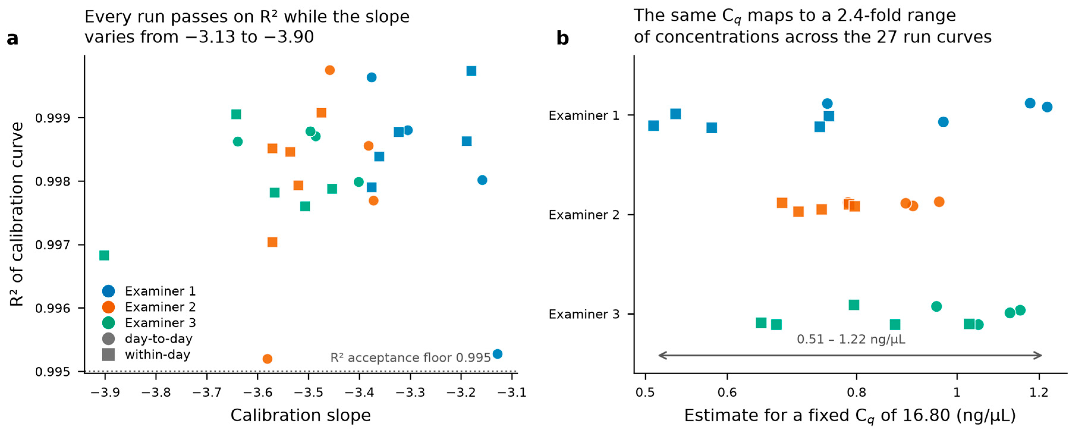
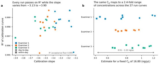
Figure 1. Calibration-curve performance across the 27 runs. (a) Coefficient of determination against slope for every run. All runs satisfy the R-squared threshold of 0.995 applied in the appraisal protocol (dotted line) while the slope varies from −3.128 to −3.902, corresponding to amplification efficiencies of 80.4% to 108.8%. (b) Concentration that each of the 27 run-specific curves assigns to one fixed quantification cycle of 16.80, close to the mean Cq of Sample B. The same Cq maps to 0.509–1.222 ng/μL, a 2.40-fold range, according only to which run supplied the curve. Circles, runs of the between-day experiment (n = 12); squares, runs of the within-day experiment (n = 15); colour denotes operator. Note the logarithmic concentration axis in panel (b). Blue, Examiner 1; orange, Examiner 2; green, Examiner 3.

3. Results

3.1. Calibration-Curve Performance and Quality Control

Across all 27 runs (12 in the between-day experiment and 15 in the within-day experiment), 243 standard reactions and 162 unknown reactions were measured. Every run met the linearity criterion of the appraisal protocol (R-squared ≥ 0.995; Section 2.2), a laboratory-specific threshold rather than a universal qPCR acceptance criterion: R-squared ranged from 0.9952 to 0.9998 (Figure 1a). The regression parameters of the curves, however, were not interchangeable. Slopes ranged from −3.128 to −3.902 (mean −3.443) and intercepts from 15.87 to 17.09, corresponding to amplification efficiencies of 80.4% to 108.8%; five runs exceeded 100% nominal efficiency, which in an intercalator-based assay is usually taken to indicate slight deviation of the dilution series or of the fit rather than genuine supra-exponential amplification. Per-run parameters are given in Sheet S2 of the Supplementary Data S1. No predefined slope or efficiency criterion applied to this system (Section 2.2). All 27 curves were retained, because the study question concerns the variability among curves that passed the checks actually in use; as a descriptive check, restricting the paired cross-run analysis to the 24 runs with efficiencies of 90–110%, an exploratory range applied only as a descriptive check and not as an acceptance criterion, left the stratum medians essentially unchanged (13.3–19.9%; Supplementary Sheet S12, Part D).

The practical consequence of this spread is shown in Figure 1b. A single quantification cycle of 16.80, close to the mean Cq of Sample B, is converted by the 27 run-specific curves into concentrations ranging from 0.509 to 1.222 ng/μL, a 2.40-fold range with a CV of 23.2% across curves; the corresponding ranges at the mean Cq of Sample A and Sample C were 2.44-fold and 2.27-fold. The spread was not attributable to one operator: curves from all three examiners, and from both experiments, are distributed across the range. R-squared was therefore uninformative about the comparability of the curves, and the variation in slope and intercept is the quantity that matters when a curve is transferred between runs.

3.2. Between-Day Precision

Pooling both duplicate reactions, the mean concentration over four days was 0.797 ng/μL (SD 0.120) for Sample A, 0.981 ng/μL (SD 0.121) for Sample B and 2.423 ng/μL (SD 0.248) for Sample C. Per operator, CV ranged from 11.4% to 19.5% for Sample A, 8.8% to 10.7% for Sample B and 7.6% to 9.7% for Sample C (Table 1). The absolute SD increased with concentration while CV did not, which is the expected behaviour of a multiplicative measurement process within this part of the working range. The largest deviation of a single measurement from its own operator-and-sample mean was 40.0% (Examiner 2, Sample A) but this is a maximum of eight observations and is reported only for comparability with the original submission; the CV and the 95% confidence intervals in Table 1 are the summary measures we rely on. Between-operator spread in the mean was 10.8% for Sample A, 18.9% for Sample B and 12.5% for Sample C; as the three examiners measured in different calendar periods, this spread is descriptive and is not an estimate of an operator effect. Dispersion did not track experience. Averaged over the three samples, the mean CV was 11.2% for Examiner 1 (approximately 5 years of experience), 13.0% for Examiner 2 (approximately 25 years) and 9.3% for Examiner 3 (approximately 15 years) between days, and 14.8%, 9.8% and 15.5% respectively within a day; the most experienced examiner had the widest dispersion of the three between days and the narrowest within a day. With three operators, and with operator confounded with calendar period, this is a description of the present dataset and not an estimate of any relationship between experience and precision.

Table 1. Between-day precision of DNA quantification by sample and operator over four consecutive days. Concentrations in ng/μL, recomputed from raw Cq with the contemporaneous calibration curve of each run. Both duplicate reactions contribute to the mean, SD, CV and range, so n = 8 reactions per cell (4 days × 2 replicates); the 95% confidence interval of the mean was calculated using the duplicate-pair mean of each run as the independent observational unit, so n = 4 runs per cell. CV, coefficient of variation; CI, confidence interval.

Sample	Operator	n Reactions	n Runs	Mean	SD	CV (%)	Range	95% CI of Mean	Mean Cq (SD)
A	Examiner 1	8	4	0.763	0.100	13.2	0.601–0.866	0.615–0.911	17.21 (0.18)
A	Examiner 2	8	4	0.779	0.152	19.5	0.609–1.090	0.615–0.943	17.01 (0.23)
A	Examiner 3	8	4	0.849	0.097	11.4	0.710–1.039	0.741–0.956	17.16 (0.15)
B	Examiner 1	8	4	0.988	0.105	10.7	0.862–1.144	0.835–1.140	16.84 (0.19)
B	Examiner 2	8	4	0.885	0.094	10.6	0.698–1.005	0.769–1.000	16.81 (0.23)
B	Examiner 3	8	4	1.070	0.094	8.8	0.924–1.206	0.916–1.223	16.80 (0.05)
C	Examiner 1	8	4	2.512	0.245	9.7	2.228–2.930	2.110–2.915	15.53 (0.14)
C	Examiner 2	8	4	2.227	0.200	9.0	1.999–2.591	1.945–2.510	15.42 (0.10)
C	Examiner 3	8	4	2.530	0.192	7.6	2.284–2.774	2.224–2.836	15.49 (0.07)

Within-run repeatability, estimated directly from the duplicate reactions that the original submission discarded, was best for the highest-concentration sample: the mean duplicate CV was 11.5% for Sample A, 5.9% for Sample B and 3.6% for Sample C, and the mean absolute Cq difference between duplicates was 0.24, 0.12 and 0.08 cycles respectively.

3.3. Within-Day Precision

In five consecutive runs on a single day, the mean concentration was 0.619 ng/μL (SD 0.099) for Sample A, 0.804 ng/μL (SD 0.123) for Sample B and 1.801 ng/μL (SD 0.272) for Sample C, with per-operator CVs of 10.5–17.3%, 7.3–13.2% and 11.7–18.7% respectively (Table 2). Mean duplicate CV was 9.4%, 4.4% and 7.2% for Samples A, B and C.

Table 2. Within-day precision of DNA quantification by sample and operator over five consecutive runs on a single day. Concentrations in ng/μL. Both duplicate reactions contribute to the mean, SD, CV and range, so n = 10 reactions per cell (5 runs × 2 replicates); the 95% confidence interval of the mean was calculated using the duplicate-pair mean of each run as the independent observational unit, so n = 5 runs per cell. Columns as in Table 1.

Sample	Operator	n Reactions	n Runs	Mean	SD	CV (%)	Range	95% CI of Mean	Mean Cq (SD)
A	Examiner 1	10	5	0.553	0.096	17.3	0.462–0.722	0.445–0.662	16.97 (0.16)
A	Examiner 2	10	5	0.653	0.068	10.5	0.554–0.791	0.604–0.703	17.00 (0.16)
A	Examiner 3	10	5	0.650	0.102	15.7	0.507–0.838	0.533–0.767	17.12 (0.14)
B	Examiner 1	10	5	0.685	0.090	13.2	0.544–0.846	0.578–0.791	16.66 (0.12)
B	Examiner 2	10	5	0.835	0.061	7.3	0.766–0.933	0.772–0.899	16.62 (0.11)
B	Examiner 3	10	5	0.892	0.108	12.1	0.761–1.007	0.751–1.033	16.62 (0.13)
C	Examiner 1	10	5	1.703	0.237	13.9	1.414–2.077	1.408–1.998	15.36 (0.13)
C	Examiner 2	10	5	1.885	0.220	11.7	1.511–2.101	1.721–2.049	15.37 (0.16)
C	Examiner 3	10	5	1.815	0.339	18.7	1.313–2.274	1.378–2.253	15.52 (0.09)

The original submission reported that within-day variation exceeded between-day variation. That comparison rested on the maximum deviation observed in five runs versus four days, and maxima are not comparable across designs with different numbers of observations. On the CV and confidence-interval measures used here, the two experiments are closely similar: the per-operator CV range was 7.6–19.5% between days and 7.3–18.7% within a day, and intermediate precision (Table 3) was 10.9–17.6% across all six sample-by-experiment combinations. We therefore no longer claim that within-day variability is larger. The mean concentrations of all three samples were, however, lower in the within-day experiment than in the between-day experiment. Because a progressive downward trend occurred across measurement occasions (Section 3.4) and its cause cannot be separated from storage, repeated sampling of the same tube, or an order effect, this difference should not be interpreted as evidence of better or poorer precision in either experiment.

Table 3. Variance components of ln-transformed DNA concentration, expressed as coefficients of variation. Estimated from a balanced nested random-effects model with operator random, run nested within operator, and the duplicate reaction as residual. Repeatability, within-run; between-run, run-to-run within one operator; intermediate precision, the combination of all three terms. The third term is labelled between-operator/period because the three examiners measured in sequence and never on the same day, so it absorbs any between-period difference as well as any between-operator difference and is not an estimate of an operator effect. Negative method-of-moments estimates were set to zero. With three operators, these estimates carry wide uncertainty.

Experiment	Sample	Repeatability CV (%)	Between-Run CV (%)	Between-Operator/Period CV (%)	Intermediate Precision CV (%)
day-to-day	A	13.7	5.7	1.9	15.0
day-to-day	B	7.7	7.3	8.5	13.6
day-to-day	C	4.9	7.8	5.8	10.9
within-day	A	10.8	10.2	7.9	16.9
within-day	B	5.7	10.3	13.0	17.6
within-day	C	9.2	13.0	0.0	16.0

3.4. Variance Components and the Trend Across Occasions

The nested random-effects analysis apportioned the total variation of ln concentration among the duplicate reaction (repeatability), the run, and the operator (Table 3). Repeatability CV was 4.9–13.7%, between-run CV 5.7–13.0% and between-operator/period CV 0–13.0%, giving an intermediate-precision CV of 10.9–17.6%. No single term dominated consistently: repeatability accounted for 84% of the variance for Sample A between days but only 11% for Sample B within a day, while the operator/period term was estimated at zero in one of the six combinations and at 1.9% CV in another. A non-zero between-run component was estimated in all six sample-by-experiment combinations. However, with three operators and four or five runs per operator, these components are imprecise; the operator term is not separable from calendar period, the run term is not separable from the progressive trend described below, and the magnitudes and the ordering of the terms should therefore be interpreted cautiously.

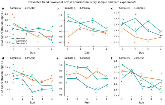
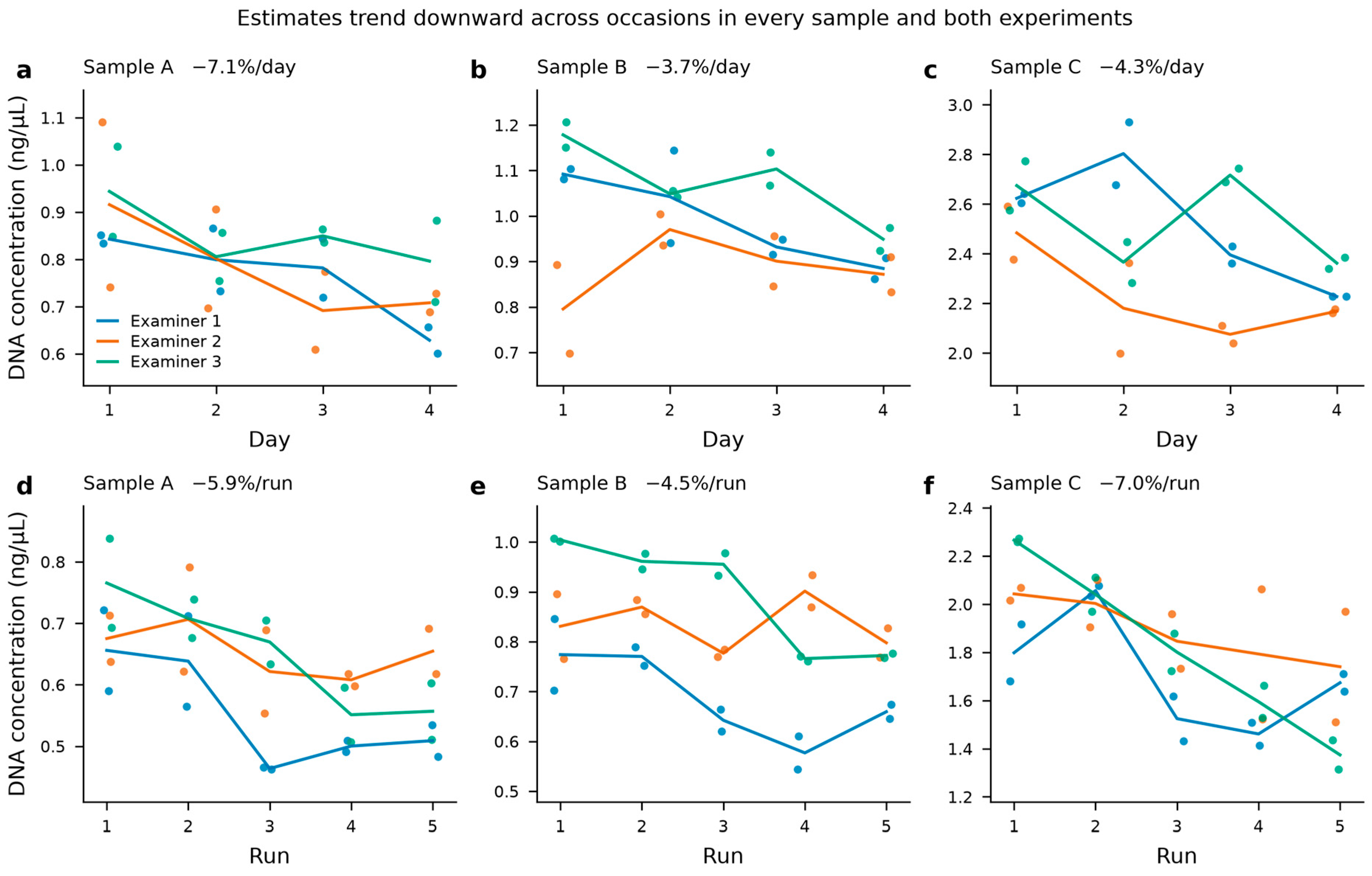
Examination of the individual measurements over successive occasions revealed a feature not reported in the original submission (Figure 2). In all six sample-by-experiment combinations the estimated concentration declined across occasions, with descriptive pooled least-squares slopes of −7.1%, −3.7% and −4.3% per day for Samples A, B and C in the between-day experiment and of −5.9%, −4.5% and −7.0% per run in the within-day experiment; over four days the total decline was 21.1%, 11.8% and 13.2%. Because each examiner’s aliquot was thawed once and then held at 4 °C and sampled repeatedly, the between-day term estimated in Table 3 necessarily conflates run-to-run measurement variation with any progressive change in the sample itself, and the same is true of the within-day term over the course of one day’s runs. This is a limitation of the design rather than a result about the assay, and it is discussed further in Section 4.3.

Figure 2. DNA concentration estimates across successive measurement occasions. (a–c) Four consecutive days; (d–f) five consecutive runs within a single day. Points are individual duplicate reactions (horizontally jittered), lines join the operator mean for each occasion, and the value in each panel heading is the descriptive least-squares trend in percent per occasion pooled over operators, shown without inferential statistics because repeated observations within an operator are not independent. Note that the vertical scale differs between panels; each panel is scaled to its own sample. The consistent downward trend means that the between-occasion term of Table 3 includes any progressive change in the stored sample as well as run-to-run measurement variation.

3.5. Effect of Applying a Calibration Curve Generated in a Different Run

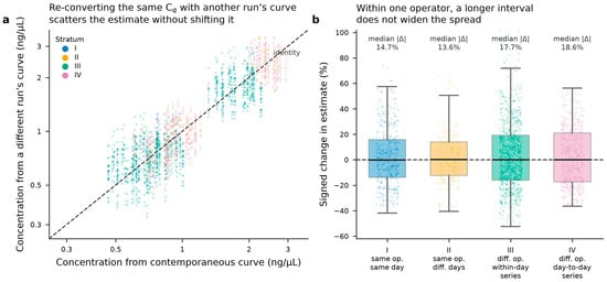
When each unknown Cq was re-converted with the calibration curve of a different run, the estimate changed by a median of 14.7% (interquartile range 7.0–27.6) for another run by the same operator on the same day, 13.6% (6.3–20.7) for a run by the same operator on a different day, 17.7% (9.2–30.1) for a run by a different operator taken from a within-day series, and 18.6% (8.5–27.0) for a run by a different operator taken from the four-day series (Table 4). Between 26% and 46% of pairings changed the estimate by more than 20%, and the largest single change was 102.4%. The mean signed change was small in every stratum, between +2% and +3%. Because the same unknown measurements and the same calibration curves are reused across many of the 2052 pairings, these pairings are not statistically independent, and a confidence interval computed as though they were would understate the true uncertainty; we therefore report the mean signed change as a descriptive summary only, without an accompanying interval. Changes occurred in both directions within every stratum (Figure 3), which is the basis for describing the effect as dispersive rather than displacing the estimate in a consistent direction; there is no general correction factor that could be applied.

Table 4. Change in the calculated DNA concentration when the same quantification cycle is converted with a calibration curve generated in a different run, by stratum. Each row summarizes all pairings of one unknown measurement (Cq held constant) with one non-contemporaneous curve from the same experiment block. Signed change = 100 × (alternative − contemporaneous)/contemporaneous; absolute change is its absolute value. Stratum I comprises pairings within one operator’s within-day series, in which the two runs were minutes to hours apart; stratum II pairings within one operator’s four-day series; and strata III and IV cross-operator pairings, which because the examiners measured in sequence are always also cross-day, distinguished by whether the substituted curve came from a within-day series (III) or the four-day series (IV). The last two columns give the proportion of pairings whose absolute change exceeded 20% and 50%, respectively. The 2052 pairings are not statistically independent, because each unknown measurement and each calibration curve contribute to many pairings; the proportions in the last two columns therefore describe the set of pairings and should not be read as frequencies of independent events.

Stratum	n Pairings	Median |Change| (%)	IQR (%)	Mean |Change| (%)	95th Percentile (%)	Maximum (%)	Mean Signed Change (%)	Pairings > 20% (%)	Pairings > 50% (%)
I. Same operator, same day	360	14.7	7.0–27.6	18.4	44.2	73.7	+2.5	40	3.3
II. Same operator, different days	216	13.6	6.3–20.7	16.2	48.1	65.7	+1.9	26	4.6
III. Different operator, different days (within-day series)	900	17.7	9.2–30.1	21.6	51.3	102.4	+3.3	45	5.8
IV. Different operator, different days (day-to-day series)	576	18.6	8.5–27.0	19.4	43.2	56.3	+2.5	46	2.8

Figure 3. Paired effect of converting the same quantification cycle with a calibration curve from a different run. (a) Each point is one unknown measurement paired with one non-contemporaneous curve (n = 2052): the concentration obtained with the contemporaneous curve on the horizontal axis against that obtained with the substituted curve on the vertical axis, both axes logarithmic, with the identity line dashed. Points fall on both sides of the identity line, indicating substantial bidirectional dispersion rather than systematic displacement. (b) Signed percentage change by stratum, with the median absolute change annotated above each box. Boxes show the median and interquartile range, whiskers the 1.5-interquartile-range limits, and individual pairings are overplotted. Stratum I, same operator, another run on the same day; II, same operator, a run on a different day; III, a different operator, curve from a within-day series; IV, a different operator, curve from the four-day series. The similarity of strata I and II indicates that, within the same operator, increasing the interval between runs from minutes or hours to different days was not associated with a larger discrepancy in this dataset. Strata III and IV are descriptive: operator identity is confounded with calendar period, so their larger values cannot be attributed to the operator.

The stratification clarifies one aspect of the question that the original design could not address. Holding the operator constant, the median absolute change was 14.7% when the substituted curve came from another run by the same operator on the same day, the two runs being separated by minutes to hours, and 13.6% when it came from a run on a different day. Thus, within the same operator, separation of the runs by days rather than minutes was not associated with a larger discrepancy. This holds for the present dataset only; because strata I and II derive from separate experimental blocks, the comparison is not a controlled estimate of an elapsed-time effect. Cross-operator pairings showed somewhat larger median absolute changes, 17.7% and 18.6%. However, because the three examiners measured sequentially and never on the same day, operator identity is fully confounded with calendar period, and these larger values cannot be attributed specifically to the operator; they are reported descriptively. Two further limits on interpretation should be stated. The within-operator comparison spans intervals of minutes to a few days, so it does not license any inference about curves stored for weeks or months, which is the situation that arises in casework. And the cross-operator strata span intervals of that longer order, so their larger values are equally consistent with a longer interval, with a change of operator, or with any change in the laboratory between one examiner’s measurement period and the next. The data therefore support the narrower conclusion that applying a calibration curve generated in a different run introduces substantial variability, while this design does not permit the independent contributions of operator identity, calendar period and elapsed time to be quantified. Accordingly, we no longer describe the finding as an effect of calibration-curve timing.

For direct comparison with the original submission, Table 5 reports the specific pairing used there, in which the Day-1 curve of one examiner is applied to another examiner’s measurements. The mean signed change ranged from −10.0% to +41.3% across the six examiner pairings and three samples, and the largest absolute change for a single measurement was 56.3%. We note that the values of approximately 48%, 50% and 52% quoted in the original submission for Samples A, B and C were the spans between the most positive and the most negative pairing for each sample (48.4, 48.4 and 50.6 percentage points on the corresponding recomputation, read directly from the mean signed changes in Table 5), not deviations from the contemporaneous result; the largest mean deviation for any single pairing is 41.3%. The text, Abstract and Conclusions have been corrected throughout, and the paired measures of Table 4 rather than any cross-pairing span are now the basis of the reported result.

Table 5. Change in mean quantification values when the Day-1 calibration curve of one examiner is applied to the measurements of another examiner, corresponding to the pairing reported in the original submission. Mean signed change and maximum absolute change over the four days and both duplicate reactions (n = 8 measurements per cell), with the Cq of each measurement held constant. Positive values indicate that the substituted curve returns the higher estimate.

Curve from	Applied to	Sample A	Sample B	Sample C
Examiner 1	Examiner 2	+38.4 (55.9)	+38.7 (55.8)	+41.3 (55.7)
Examiner 1	Examiner 3	+13.7 (27.6)	+14.8 (28.1)	+18.8 (32.2)
Examiner 2	Examiner 1	−1.5 (31.0)	−3.3 (26.5)	−9.3 (22.8)
Examiner 2	Examiner 3	−10.0 (16.3)	−9.7 (16.5)	−8.6 (17.7)
Examiner 3	Examiner 1	+17.4 (56.3)	+15.7 (51.8)	+10.2 (40.7)
Examiner 3	Examiner 2	+30.4 (47.0)	+30.6 (46.6)	+32.1 (45.5)

3.6. Sensitivity of the Results to Calibration-Curve Construction

When the 0.001 ng/μL point was excluded and the curves were refitted to the four manufacturer-range standards (10 to 0.01 ng/μL) of the first replicate, exactly as in the primary analysis, the results were essentially unchanged. Slopes ranged from −3.701 to −3.169 (amplification efficiency 86.3–106.8%, five runs above 100%), and the fixed Cq of 16.80 was converted into 0.508–1.219 ng/μL, a 2.40-fold range with a CV of 23.2% across curves, identical to the primary model. In the paired cross-run analysis, the median absolute change was 15.1% (interquartile range 7.1–27.7) in stratum I, 13.5% (6.6–20.9) in stratum II, 18.0% (8.8–29.8) in stratum III and 18.1% (8.9–26.7) in stratum IV, with a maximum of 103.0%, against 14.7%, 13.6%, 17.7% and 18.6% under the primary model; the ordering of the four strata was preserved, changes occurred in both directions in every stratum, and the absolute changes of individual pairings under the two models were almost perfectly correlated (Spearman rho 0.99). The R-squared values of these retrospective four-point fits ranged from 0.9929 to 0.9996; one fit (Examiner 2, Day 2) fell below the threshold of 0.995 that had been applied to the original five-point curves. Because these four-point curves were fitted retrospectively for sensitivity analysis and were not used for run acceptance, that threshold was not reapplied as an exclusion criterion; omitting that run left the stratum medians at 15.1–18.1%. Intermediate-precision CV was 10.2–17.6% against 10.9–17.6%, and contemporaneous concentrations differed from the primary values by a median of 0.0% (range −4.1% to +3.6%). The additional point therefore did not drive any of the principal results. The secondary alternative model, fitted to the mean Cq of the duplicate standards at the four manufacturer-range concentrations, gave a similar fixed-Cq range (2.38-fold) and somewhat smaller cross-run discrepancies (stratum medians 10.5–16.2%, maximum 101.8%); the same-operator strata again showed lower median changes than the cross-operator strata, although the order of strata III and IV was reversed. Because that model changes the replicate treatment as well as the number of points, the smaller discrepancies cannot be attributed to the exclusion of the 0.001 ng/μL point. Neither model altered any substantive conclusion. The complete comparison is given in Supplementary Sheets S11 and S12.

4. Discussion

4.1. Analytical Precision of the Tested System

In this single instrument–assay system, the precision of real-time PCR quantification, expressed as intermediate-precision CV, was between 11% and 18% depending on the sample, with within-run repeatability CV of 5–14% and a between-operator/period CV of up to 13% that cannot be resolved into an operator component and a period component. These are estimates of dispersion, not of agreement with a true value: no reference material of assigned concentration was measured, so no statement about trueness or accuracy can be made from these data, and we have accordingly replaced the language of “measurement error” used in the original submission with repeatability, intermediate precision and between-operator/period precision throughout. Non-negligible within- and between-operator imprecision of manual pipetting has been reported in recent studies [17,18], and the broader observation that quantitative results can differ between operators and between runs even when the same kit and principle are used is consistent with performance-evaluation studies of commercial quantification kits [13,14].

One consequence deserves emphasis for practitioners. Because the duplicate reactions carry a repeatability CV of 5–14%, the mean of a duplicate pair, which is the value a casework report would normally carry, is itself an estimate with a confidence interval of practical width. Reporting a quantification result as a single number without an associated interval understates what is known about it, and MIQE 2.0 [12] now makes explicit the reporting elements needed for a reader to judge this. The CVs and confidence intervals reported here characterize this dataset and this instrument–assay system; they are study-specific precision estimates, not a complete measurement-uncertainty model across sample types, concentration ranges and operational conditions, and uncertainty or precision statements for casework should be derived from each laboratory’s own validation and ongoing performance data over the relevant analytical range.

4.2. Transfer of a Calibration Relationship Between Runs

The principal finding of the revised analysis is that the Cq-to-concentration relationship of this assay is not stable enough across runs for a stored calibration equation to be substituted without consequence. All 27 curves would have passed an R-squared-based acceptance check, yet their slopes spanned 80.4% to 108.8% amplification efficiency, and one fixed Cq was converted by them into concentrations differing by a factor of 2.4. In paired terms, substituting a curve from another run moved the estimate by a median of 14–19% (essentially unchanged when the 0.001 ng/μL standard was excluded from the curves; Section 3.6) and, in the tail of the distribution, by more than 50%.

Two features of this result matter for how it should be used. First, the effect is dispersive: the changes occurred in both directions, and the mean signed changes were small relative to the corresponding mean absolute changes; because the underlying pairings are not statistically independent, we report these mean signed changes descriptively rather than with a confidence interval. The practical implication is an increase in uncertainty rather than a predictable shift. Second, within the same operator, the magnitude was similar whether the substituted curve came from another run performed minutes to hours apart or from a run performed on a different day, although, because the two strata come from separate experimental blocks, this is not a controlled estimate of the effect of elapsed time. Cross-operator pairings showed somewhat larger discrepancies, but operator identity is fully confounded with calendar period and therefore cannot be identified as the cause of that increase. This also gives the manufacturer’s instruction an empirical footing: the package insert requires a curve to be prepared in each run, and our data show why a departure from that instruction cannot be treated as a formality, since the resulting shift is of a size that would be material to any quantitative conclusion drawn from the result. The original submission attributed the effect to the timing of curve preparation; the stratified reanalysis does not support such a specific causal attribution. The finding is more appropriately described as variability introduced when a calibration relationship is transferred between separate amplification runs. We would add one caution against the opposite over-reading: the within-operator comparison covers intervals of minutes to a few days only, so it is evidence that the discrepancy does not grow over that span, not evidence that a curve may safely be stored and reused after weeks or months. This is also why R-squared, which describes the fit of one curve to its own standards, cannot serve as a check on transferability, and why the slope, intercept and efficiency of each run should be recorded whenever a curve might later be reused.

4.3. Candidate Mechanisms That Remain Untested

The design of this study does not identify the source of either the observed imprecision or the run-to-run instability of the curves, and we present the candidate mechanisms explicitly as hypotheses. Small differences in the volume of template or standard dispensed with a micropipette are one plausible contributor and would be consistent with the published imprecision of manual pipetting [17,18]; however, we did not measure dispensed volumes, did not compare manual with electronic pipetting, and did not hold the other candidate sources constant, so the pipetting hypothesis is not tested by these data. The original submission’s inference that high R-squared implicated pipetting of unknown samples specifically is not sound: a high R-squared shows only that the standard points lie close to a straight line, and is compatible with a systematically mis-diluted standard series, which would shift slope and intercept while leaving the fit excellent. Our own observation that R-squared was uniformly high while slopes varied over an efficiency range of 80–109% illustrates the point directly, and indeed makes preparation of the standard dilution series at least as plausible a contributor as pipetting of the unknowns. Other candidates that these data cannot separate include run-to-run differences in amplification efficiency arising from reagent handling, the threshold and baseline determination applied by the instrument software, well-to-well thermal or optical differences within the instrument, and the stability of reagents and standards after opening. A suitably designed follow-up study would vary these one at a time, and the evaluation of electronic pipettes is a reasonable element of such a study, but it is future work rather than a corrective measure supported by the present experiment.

The progressive decline in estimated concentration across occasions (Figure 2) is itself a candidate mechanism for part of what was previously reported as between-day variation. Each examiner’s aliquot was thawed once and then held at 4 °C and sampled on each of four days, so any loss, adsorption or degradation during storage would appear as a downward between-day trend, and a decline of 12–21% over four days is of the order that has to be taken seriously. The same trend appeared within a single day, where storage time is short, so it is unlikely to be the whole explanation; repeated sampling of the same tube, evaporation, or an order effect over successive runs could all contribute. Because run order was fixed and not randomized, a fatigue or order effect cannot be separated from a storage effect in these data. We raise this as a limitation of the design and as an argument for randomizing run order and using a fresh aliquot per occasion in any future study, rather than as a demonstrated cause.

4.4. Forensic Applicability and Limitations

The findings apply to the specific analytical system tested, a SmartCycler II with the Human Genomic DNA Quantification Kit Ver. 2, and to clean oral-swab extracts within the concentration range examined. They should not be generalized to other quantification platforms, to other kits, or to the low-template, degraded, inhibited and heterogeneous material typical of trace casework, in which precision is expected to be poorer, particularly near the limit of quantification. None of our samples was a low-template sample in that sense.

It also needs to be stated plainly that analytical imprecision is only one of the components of uncertainty that bear on the evidential interpretation of a DNA quantity. The amount of DNA measured in an extract is separated from the event in dispute by deposition, transfer and persistence, by the efficiency of sampling from the substrate, by extraction recovery, and by degradation and inhibition, each of which contributes its own and generally larger uncertainty. The present experiments say nothing about any of these, and a measured DNA quantity does not establish the mechanism or the time of deposition. Our results speak to a narrower but tractable question: given a Cq obtained on this system, how much does the reported concentration depend on which run supplied the calibration curve, and how reproducible is the measurement between operators and runs. In the case that motivated the study, the first-instance court noted that the calibration data and the extract had been discarded and could not be independently checked. Our finding that the choice of run-specific curve alone can move the reported value by a median of 14–19%, and occasionally by more than 50%, is a concrete reason why the calibration data of the same run, the run-specific slope and intercept, and the identity of the run that generated the curve should be preserved and disclosed whenever a quantitative DNA result may be weighed as evidence.

The study has several further limitations. Only three samples, three operators and one instrument-and-kit combination were examined, the last constrained by the 16 wells of the SmartCycler II, 10 of which were required for the five-point calibration series. With three operators, the between-operator/period variance component is estimated with wide uncertainty and its ordering relative to the other terms should not be relied upon. No trueness or accuracy assessment was possible in the absence of a characterized reference material. Because the three examiners measured in sequence and never on the same day, the operator is fully confounded with calendar period and with the source of the curve, which is why the stratified analysis of Section 3.5, and within it the comparison of strata I and II, rather than the original pairwise comparison, carries the argument; a between-operator difference estimated from this design cannot be separated from any change in the laboratory or in the samples between one examiner’s measurement period and the next. Two of the three donors were also examiners, although this is not expected to affect precision. Run order was fixed, the between-day aliquots were stored at 4 °C after a single thaw, and the additional 0.001 ng/μL standard was not independently validated, although a sensitivity analysis excluding it did not change the substantive conclusions (Section 3.6). Finally, the analysis is retrospective with respect to an appraisal conducted for a specific legal proceeding, and the design was shaped by the question put to that appraisal rather than by the requirements of a validation study.

5. Conclusions

In real-time PCR-based human DNA quantification with a SmartCycler II and the Human Genomic DNA Quantification Kit Ver. 2, the intermediate precision of the measurement was 11–18% CV, with within-run repeatability of 5–14% and a between-operator/period term of up to 13% CV, for clean oral-swab extracts of 0.46–2.93 ng/μL. Converting a quantification cycle with a calibration curve generated in a different run changed the reported concentration by a median of 14–19%, exceeded 20% in approximately one quarter to one half of pairings, and in the extreme exceeded 100%; these findings were substantively unchanged when the unvalidated 0.001 ng/μL standard was excluded from the calibration curves. The changes were predominantly dispersive rather than consistently directional. Within the same operator, the magnitude of the discrepancy was similar whether the substituted curve came from another run on the same day or from a run on a different day. Because operator identity was fully confounded with calendar period, the independent contribution of the operator could not be determined from this design. Every one of the 27 calibration curves satisfied an R-squared criterion of 0.995 while the slopes corresponded to amplification efficiencies from 80% to 109%, so linearity of fit is not a sufficient check on whether a curve may be reused. Within the limits of this single-system, preliminary study, the practical implications are that a calibration curve should be generated in the same run as the unknown it is used to convert, that slope, intercept, efficiency and the underlying Cq values should be recorded and preserved, and that a quantification result intended to carry evidential weight should be accompanied by an explicit statement of its precision, derived from the laboratory’s own validation and performance data rather than from the study-specific estimates reported here.

References

- Supreme Court of Japan, Second Petty Bench. Judgment of 18 February 2022 (Case of Quasi-Forced Indecency). Available online: https://www.courts.go.jp/app/hanrei_jp/detail2?id=90933 (accessed on 10 July 2026).
- Bengo4.com News. Supreme Court Quashes High Court’s Guilty Verdict in Breast Surgeon’s Quasi-Forced Indecency Case, Remands for Retrial. Bengo4.com News, 18 February 2022. Available online: https://www.bengo4.com/c_1009/n_14135/ (accessed on 10 July 2026). (In Japanese)
- Nikkei Medical Online. Never Repeat the Tragedy: Looking Back on the Trial of a Breast Surgeon Prosecuted for Quasi-Forced Indecency; April 2025. Available online: https://medical.nikkeibp.co.jp/leaf/mem/pub/report/202504/588187.html (accessed on 10 July 2026). (In Japanese)
- Gill, P.; Whitaker, J.; Flaxman, C.; Brown, N.; Buckleton, J. An investigation of the rigor of interpretation rules for STRs derived from less than 100 pg of DNA. Forensic Sci. Int. 2000, 112, 17–40. [Google Scholar] [CrossRef] [Scilit]
- Lee, S.B.; McCord, B.; Buel, E. Advances in forensic DNA quantification: A review. Electrophoresis 2014, 35, 3044–3052. [Google Scholar] [CrossRef] [Scilit]
- Versmessen, N.; Van Simaey, L.; Negash, A.A.; Vandekerckhove, M.; Hulpiau, P.; Vaneechoutte, M.; Cools, P. Comparison of DeNovix, NanoDrop and Qubit for DNA quantification and impurity detection of bacterial DNA extracts. PLoS ONE 2024, 19, e0305650. [Google Scholar] [CrossRef] [Scilit]
- Heid, C.A.; Stevens, J.; Livak, K.J.; Williams, P.M. Real time quantitative PCR. Genome Res. 1996, 6, 986–994. [Google Scholar] [CrossRef] [Scilit]
- Nicklas, J.A.; Buel, E. Development of an Alu-based, real-time PCR method for quantitation of human DNA in forensic samples. J. Forensic Sci. 2003, 48, 936–944. [Google Scholar] [CrossRef] [Scilit]
- Alonso, A.; Martin, P.; Albarran, C.; Garcia, P.; Garcia, O.; Fernandez de Simon, L. Real-time PCR designs to estimate nuclear and mitochondrial DNA copy number in forensic and ancient DNA studies. Forensic Sci. Int. 2004, 139, 141–149. [Google Scholar] [CrossRef] [Scilit]
- McDonald, C.; Taylor, D.; Linacre, A. PCR in forensic science: A critical review. Genes 2024, 15, 438. [Google Scholar] [CrossRef] [Scilit]
- Bustin, S.A.; Benes, V.; Garson, J.A.; Hellemans, J.; Huggett, J.; Kubista, M.; Mueller, R.; Nolan, T.; Pfaffl, M.W.; Shipley, G.L.; et al. The MIQE guidelines: Minimum information for publication of quantitative real-time PCR experiments. Clin. Chem. 2009, 55, 611–622. [Google Scholar] [CrossRef] [Scilit]
- Bustin, S.A.; Ruijter, J.M.; van den Hoff, M.J.B.; Kubista, M.; Pfaffl, M.W.; Shipley, G.L.; Tran, N.; Roediger, S.; Untergasser, A.; Mueller, R.; et al. MIQE 2.0: Revision of the Minimum Information for Publication of Quantitative Real-Time PCR Experiments guidelines. Clin. Chem. 2025, 71, 634–651. [Google Scholar] [CrossRef] [Scilit]
- Lin, S.W.; Li, C.; Ip, S.C.Y. A performance study on three qPCR quantification kits and their compatibilities with the 6-dye DNA profiling systems. Forensic Sci. Int. Genet. 2018, 33, 72–83. [Google Scholar] [CrossRef] [Scilit]
- Harrel, M.; Mayes, C.; Houston, R.; Holmes, A.S.; Gutierrez, R.; Hughes, S. The performance of quality controls in the Investigator Quantiplex Pro RGQ and Investigator 24plex STR kits with a variety of forensic samples. Forensic Sci. Int. Genet. 2021, 55, 102586. [Google Scholar] [CrossRef] [Scilit]
- QIAGEN. QIAamp DNA Mini and Blood Mini Handbook; QIAGEN: Hilden, Germany; Available online: https://www.qiagen.com/us/resources/download.aspx?id=62a200d6-faf4-469b-b50f-2b59cf738962&lang=en (accessed on 23 September 2026).
- Jaeger, R. Genomic multicopy loci targeted by current forensic quantitative PCR assays. Genes 2024, 15, 1299. [Google Scholar] [CrossRef] [Scilit]
- Guan, X.L.; Chang, D.P.S.; Mok, Z.X.; Lee, B. Assessing variations in manual pipetting: An under-investigated requirement of good laboratory practice. J. Mass Spectrom. Adv. Clin. Lab 2023, 30, 25–29. [Google Scholar] [CrossRef] [Scilit]
- Lippi, G.; Lima-Oliveira, G.; Brocco, G.; Bassi, A.; Salvagno, G.L. Estimating the intra- and inter-individual imprecision of manual pipetting. Clin. Chem. Lab. Med. 2017, 55, 962–966. [Google Scholar] [CrossRef] [Scilit]
Disclaimer/Publisher’s Note: The statements, opinions and data contained in all publications are solely those of the individual author(s) and contributor(s) and not of MDPI and/or the editor(s). MDPI and/or the editor(s) disclaim responsibility for any injury to people or property resulting from any ideas, methods, instructions or products referred to in the content. |
© 2026 by the authors. Licensee MDPI, Basel, Switzerland. This article is an open access article distributed under the terms and conditions of the Creative Commons Attribution (CC BY) license.