


Abstract
Reliable mapping of mine tailings deposits from unmanned aerial vehicle (UAV) products requires evaluation protocols that separate within-site interpolation from transfer to geographically unseen deposits. This study evaluates an eight-channel multiband segmentation workflow for six mining environments in Hidalgo, Mexico, using 4531 aligned -pixel tiles and nine overlapping semantic annotations. The quantitative analysis focuses on tailings and slope. U-Net and MobileNetV3-Large + Lite Reduced Atrous Spatial Pyramid Pooling (LR-ASPP) are assessed using a reproducible tile-level split (70/15/15, seed 42), six-fold leave-one-site-out (LOSO) validation with three seeds, a full six-site, three-seed A1–A6 input band ablation and a common-hardware benchmark. On the reproducible fixed split, MobileNetV3-Large + LR-ASPP outperforms U-Net in the global branch for tailings (Dice 0.9462 vs. 0.8944) and slope (0.7525 vs. 0.7214), while the class-specific MobileNetV3 tailings branch reaches a Dice score of 0.9507, confirming consistent performance for the tailings class. Under the stricter LOSO protocol, the tailings Dice is essentially tied (0.7356 for MobileNetV3 and 0.7361 for U-Net), whereas the slope Dice is 0.4878 and 0.4703, respectively. Each architecture ranks first at three of the six sites for both labels, and paired Wilcoxon tests on site-level means do not indicate systematic architecture dominance (). On an NVIDIA A100-SXM4-40GB benchmark, U-Net is faster (349.5 vs. 112.7 tiles/s), whereas MobileNetV3 uses 20.1% less peak measured graphics processing unit (GPU) memory. Reproducible digital terrain model (DTM)-referenced geometric postprocessing produces similar area estimates but greater sensitivity in volume. In the 216-job global model band ablation, the RGB+Z+D+ configuration without (A4) reaches the highest mean tailings Dice for U-Net (0.7452) and MobileNetV3 (0.7582). Adding local relative to A3 improves the mean slope Dice by 0.2292 and 0.0903, respectively, with the same positive direction at all six sites; no five-contrast Holm-adjusted Wilcoxon result is significant at 0.05. The results indicate that geographic domain shift dominates a simple architecture ranking; external deposits, independent annotation and survey-grade geometric references remain necessary before operational use.
1. Introduction
Mine tailings deposits are persistent mining legacies whose exposed surfaces, embankments and drainage pathways can evolve under erosion, oxidation, vegetation growth and anthropogenic disturbance. Their environmental and geotechnical relevance arises not only from residue chemistry, but also from deposit configuration, slope condition and interaction with adjacent land cover [1,2,3]. In historical mining districts such as Hidalgo, Mexico, mineralogical, geochemical and metallurgical studies have documented heterogeneous residues containing potentially hazardous and economically valuable elements [4,5,6,7,8,9,10,11,12]. Digital image analysis has also been used to characterize mineral surfaces in related regional studies [13]. Repeated spatial characterization is therefore needed to complement laboratory analyses and conventional field inspection.
To address this need, high-resolution unmanned aerial vehicle (UAV) surveying offers a practical means of repeatedly capturing the spatial and geometric characteristics of mine tailings deposits. UAV photogrammetry provides centimetric-to-decimetric orthomosaics, digital surface models (DSM), digital terrain models (DTM) and dense point clouds at a cost and operational scale compatible with repeated local surveys. These products have supported tailings surveillance, displacement analysis and stockpile volumetry [14,15]. UAV imagery combined with deep learning has also shown value for high-resolution environmental mapping in Mexico [16]. Nevertheless, converting photogrammetric products into reproducible semantic maps remains challenging. Tailings may resemble natural bare soil, roads or construction fill; slopes can be narrow, fragmented and partially covered by vegetation; and the same semantic region may exhibit strong spectral changes across deposits. Furthermore, geometric quantities derived from segmentation depend on both the elevation model and the spatial regularity of the predicted contour.
These limitations motivate the use of automated semantic segmentation methods to delineate mine tailings features directly from UAV-derived imagery. Deep convolutional networks offer an efficient alternative to exhaustive manual delineation, but architecture choice is not neutral. U-Net transfers high-resolution features through encoder–decoder skip connections and is therefore a strong reconstruction reference for irregular regions and narrow structures [17]. MobileNetV3-Large uses inverted residuals, depth-wise separable convolutions, squeeze-and-excitation and hardware-aware design. MobileNetV3-Large combined with Lite Reduced Atrous Spatial Pyramid Pooling (LR-ASPP) provides a compact multiscale segmentation pathway, which may be advantageous for broad semantic regions and memory-constrained inference [18,19]. A direct comparison is scientifically relevant because tailings delineation contains both region-level and contour-level requirements; however, contour complexity alone does not establish boundary accuracy without an independent reference.
Beyond architecture selection, the reliability of reported segmentation performance also depends on how generalization is evaluated. A related challenge is the evaluation design. Random tile splits can place neighboring portions of the same orthomosaic in both training and test partitions. Even when tiles do not overlap, they may share illumination, camera calibration, mineral texture, terrain range and spatial context, producing optimistic estimates of transferability. Site-held-out evaluation is therefore necessary to distinguish within-site interpolation from application to a geographically distinct deposit. This issue is particularly important in UAV remote sensing, where spatial autocorrelation can be stronger than in conventional image benchmarks [20,21,22].
The objective of this study is to determine how two complementary segmentation architectures exploit multiband UAV information for tailings and slope mapping, how their performance changes under site-held-out evaluation and how the resulting segmentation masks propagate into computational geometric indicators. The study makes four contributions: First, it organizes a six-site, eight-channel UAV dataset with nine overlapping semantic annotations, while the quantitative analysis focuses on tailings and slope. Second, it adapts U-Net and MobileNetV3-Large + LR-ASPP to the same multilabel representation and evaluates global and class-specific branches. Third, it combines a fixed tile-level test set, three-seed leave-one-site-out (LOSO) evaluation and a full six-fold, three-seed A1–A6 input band ablation for both architectures, making the contribution of direct coordinates, elevation, relative height and gradient descriptors assessable across all six deposits. Fourth, it quantifies inter-model sensitivity in planimetric area, terrain-following surface area and volume above a computational reference surface.
Three hypotheses guide the analysis: (H1) proposes that elevation-derived descriptors improve segmentation for some targets relative to red–green–blue (RGB) input alone. The full six-site A1–A6 study assesses this hypothesis across three seeds and two models; however, its descriptive benefits must be distinguished from multiplicity-adjusted statistical significance. (H2) states that MobileNetV3-Large + LR-ASPP provides a computationally efficient alternative, particularly for broad region delineation and GPU memory usage, whereas U-Net provides a high-resolution decoder reference with potentially different contour characteristics. (H3) assumes that site-held-out segmentation scores are substantially lower than tile-level scores because tile-level evaluation benefits from spatial and acquisition-related similarities among samples from the same site.
2. Related Work
2.1. UAV Photogrammetry for Tailing Monitoring
UAV-based Structure-from-Motion and Multi-View Stereo have become established tools for reconstructing mine surfaces at high spatial resolution. Prior studies have used these products to monitor tailings impoundments, estimate displacement and calculate stockpile or waste volumes [14,15,23]. The reliability of such measurements depends on image overlap, camera calibration, georeferencing and the distribution of ground control or independent checkpoints [24,25,26]. These studies provide the geometric foundation for the present workflow, but most do not jointly evaluate multilabel semantic segmentation and the sensitivity of downstream geometry to the segmentation architecture.
2.2. Deep Learning for Mining and Irregular Surface Mapping
Deep learning has been applied to mine and tailings dam detection in satellite imagery, UAV-based solid waste mapping, mine restoration segmentation and extraction of tailings pond surface features [21,22,27,28]. These applications demonstrate that convolutional and transformer-based models can learn complex anthropogenic surfaces, but their tasks differ in spatial scale, target ontology and validation protocol. Satellite detection emphasizes broad spatial search, whereas UAV segmentation requires accurate local boundaries and must accommodate centimetric-to-decimetric texture variation.
Taghipour et al. [29] reviewed artificial intelligence for mineral exploration, including foundation models and cross-region transfer learning. Although mineral prospectivity mapping differs from UAV tailings segmentation, the review identifies geographic transfer and heterogeneous geoscientific inputs as relevant open challenges; it therefore motivates spatially separated validation rather than providing a directly comparable segmentation baseline.
U-Net remains a standard high-resolution reference because skip connections recover spatial detail that may be lost during downsampling [17]. MobileNetV3-Large + LR-ASPP represents a different design point: a compact backbone and a lightweight context head intended to reduce activation and computational cost [19]. Comparing these models under identical semantic outputs is more informative than comparing isolated headline scores from unrelated studies. It allows the analysis to connect architecture bias with the physical scale of the target: large connected tailings regions, narrow slope faces and sparse contextual classes.
2.3. Unresolved Validation Gap
The principal methodological gap is the separation between within-site performance and geographic generalization. Many UAV datasets are divided at the image or tile level, which can preserve strong spatial dependence across subsets. This concern is consistent with established cross-validation guidance for spatially structured data, for which random partitioning can underestimate predictive error [30]. In addition, accuracy is often reported without input band ablation or common-hardware resource measurements.
The present study addresses these limitations through site-level folds, repeated seeds, thresholds selected on validation data and fixed before testing, area under the precision–recall curve (AUPRC, also referred to as PR-AUC), a full six-site, three-seed controlled input ablation and a common-server benchmark. Independent external deposits and survey-grade geometric references remain outside the current evidence and are treated explicitly as limitations rather than inferred from internal results. To synthesize the current literature landscape and highlight the methodological contributions of this study, Table 1 presents a positioning overview comparing previous work in UAV photogrammetry, satellite remote sensing and deep learning segmentations against our proposed approach.
Table 1.
Positioning of the present study relative to representative UAV, remote sensing and tailings monitoring literature. Metrics are not directly comparable across tasks or spatial scales.
As shown, while the cited studies have addressed specific aspects of mine monitoring or general semantic segmentation, there remains a distinct gap relating to unified workflows that combine multiband UAV terrain inputs with site-held-out cross-validation strategies and downstream geometric characterization.
3. Materials and Methods
Figure 1 presents the general eight-stage framework: (I) the real-time kinematic (RTK) system for ground control points (GCPs); (II) assignment of GCPs in the region of interest (ROI); (III) UAV trajectory within the ROI; (IV) photogrammetry; (V) multiband raster; (VI) deep learning model training; (VII) model inference and segmentation; and (VIII) report.
Figure 1.
General eight-stage workflow. The green-shaded region identifies the stages addressed in this paper: IV, photogrammetry; V, multiband raster; VI, deep learning model training; VII, model inference and segmentation; and VIII, report. Stages I–III document the upstream RTK/GCP georeferencing and UAV acquisition provenance.
The green-shaded region of the framework identifies the scope addressed in this paper, namely, stages IV–VIII. Stages I–III are retained to document the upstream image acquisition and georeferencing provenance that feed Stage IV, without claiming survey-grade geometric validation. Image acquisition across the six study areas utilizes a portable DJI Mini 5 Pro (DJI, Shenzhen, China) equipped with a 1-inch 50-megapixel (MP) CMOS sensor and a 24 mm equivalent lens. The flights are executed following a nadir grid with an 80% forward and 80% lateral overlap target for challenging or homogeneous terrain, while a Pixhawk-based rover featuring u-blox ZED-F9P multiband RTK GNSS receivers (u-blox AG, Thalwil, Switzerland) and an RFD900-class telemetry link (RFD900 radio family developed by RFDesign Pty Ltd., Archerfield, QLD, Australia) provides ground-point positioning, as RTK GNSS configurations materially influence photogrammetric accuracy [24,25,26]. This subsystem is described only to establish the provenance of the data; this study does not claim survey-grade geometric validation.
In Stage IV, OpenDroneMap 3.5.5 generates orthomosaics, DSMs and DTMs, which Stage V aligns into multiband rasters with resolutions between 0.0883 and 0.1845 m to extract tiles. Finally, Stage VI conducts deep learning model training and site-held-out cross-validation, Stage VII performs model inference and segmentation and Stage VIII generates the final semantic and geometric outputs. The dataset used in this work contains 4531 tiles, and their distribution and aligned raster ground sampling distance (GSD) are summarized in Table 2. Aligned GSD varies from 0.0883 to 0.1845 m/pixel, which is a 2.09-fold range. Thus, a 256-pixel tile spans approximately 22.60–47.23 m along either horizontal axis across sites; structures of equal physical width occupy different numbers of pixels. This difference is a possible contributor to domain shift, not an independently quantified causal effect. A GSD-controlled or resampled comparison would be necessary to isolate its contribution.
Table 2.
Composition of the six-site dataset and aligned raster resolution used for model development and evaluation.
3.1. Study Design and Photogrammetry
Operations were planned according to the Mexican Official Standard (Norma Oficial Mexicana, NOM) NOM-107-SCT3-2019. Ground control was established using the Instituto Nacional de Estadística y Geografía (INEGI) Red Geodésica Nacional (RGN) as the geodetic reference [31]. The official geodetic control located in the vicinity of each mine tailings survey area was used to establish the local reference for the RTK observations. From this reference, RTK GNSS equipment was used to survey the GCPs distributed within each area of interest.
Approximate WGS 84 center coordinates for all six sites are available in the published HidalgoTailings-UAV v1.0 Zenodo record [32] and are mapped in Figure 2. The approximate centers do not establish site-specific survey footprints or aerial coverage; these require georeferenced orthomosaic boundaries, which are not available in the organized records.
Figure 2.
Approximate study site centers in geographic WGS 84 coordinates based on the publicly described HidalgoTailings-UAV dataset [32]. Inset views distinguish the Pachuca–Omitlán and Zimapán area groups. These centers are not survey footprints or certified boundaries.
The GCPs were physically marked on the ground using high-visibility targets that could be clearly identified in the UAV imagery and subsequently incorporated into photogrammetric processing for georeferencing. These control points are used as part of the image orientation and georeferencing procedure and are not treated as independent photogrammetric checkpoints; therefore, the present study does not claim survey-grade absolute positional accuracy or report independent-checkpoint RMSE. The downstream workflow progresses through photogrammetry and model evaluation at six representative sample sites, CEUNI/Jales de Jaltepec, Omitlán, La Sabina, Venta Prieta, SAGO/La Alberca and Zimapán, which together incorporate diversity in oxidation, mineral texture, vegetation cover, illumination, land use and relief.
The site centers indicate that La Sabina, SAGO/La Alberca and Zimapán Zim lie in the same local geographic cluster. Consequently, six LOSO folds do not necessarily represent six geologically independent regions; geographic transfer must be interpreted in this regional context.
To illustrate the topographic complexity and environmental diversity in the study locations, Figure 3 shows the normalized three-dimensional surface models for each of the six mine tailings sites surveyed.
Figure 3.
Normalized three-dimensional surface models of the six mine tailings sites analyzed in this study: (a) CEUNI/Jales de Jaltepec, (b) Omitlán, (c) La Sabina, (d) Venta Prieta, (e) SAGO/La Alberca and (f) Zimapán. The normalized representations illustrate the relative surface morphology and topographic variability among the surveyed tailings deposits.
These normalized representations highlight the notable variations in surface morphology, relief and slope gradients among the sites, ranging from the steep irregularities of Omitlán and CEUNI to the relatively flat deposits of Venta Prieta and SAGO, providing the physical context for the subsequent photogrammetric and deep learning segmentation analyses.
3.2. Multiband Representation and Multilabel Ontology
Each tile contains an eight-channel feature vector, as defined in (Equation (1)):
where denotes the feature vector at raster pixel , i and j are the row and column indices and , and are the red, green and blue orthomosaic values, respectively. and are normalized map coordinates, is the normalized DSM elevation, is relative height and is the normalized local elevation gradient descriptor. The representation is designed to combine material appearance with absolute/relative spatial context and local morphology, as illustrated in Figure 4. The figure has been revised to display all eight channels, including , which was omitted from the previous visual legend. For the confirmatory LOSO runs, statistics fitted to the training partition are applied unchanged to validation and held-out testing; no held-out distribution is used to recompute fitted moments. This distinction is essential for spatial variables () and topographic descriptors (), which can vary in distribution between deposits. The local gradient channel is constructed from the elevation surface using a per-tile normalized gradient descriptor before the training statistics transformation; this local operation and the train-only fitted transformation are separate steps. The operational full-raster workflow additionally records per-case 1st–99th percentile scaling for RGB, DSM and DSM–DTM, which is reported separately from the controlled model comparison.
Figure 4.
Eight-channel input representation combining RGB appearance, normalized spatial coordinates and elevation-derived descriptors.
A dedicated 2D manual labeling program was developed to generate the reference masks. The annotation process was performed manually using the orthophoto, DSM and DTM as complementary visual inputs. The ground sampling distance (GSD) was considered to ensure consistent spatial interpretation and labeling. This approach enables the manual identification and delineation of the target features. The resulting masks were used as pixel-wise reference labels for model training and evaluation. The extracted manifest confirms 4531 matched feature–mask tiles across the six sites. This file pairing check does not establish annotator identities, independent adjudication or annotation reliability.
The annotation is encoded as an overlapping bit mask: tailings = 1, slope = 2, crack = 4, water = 8, vegetation = 16, trees = 32, road = 64, building = 128 and car = 256. For class c with bit value , the corresponding binary target is obtained using Equation (2):
Here, denotes the binary target for class c on pixel , while represents the original multilabel integer mask and is the bit assigned to class c. The operator is the indicator function, which returns 1 when the condition is true and 0 otherwise, and & denotes the bitwise AND operator.
Because several labels can coexist at a pixel, the global networks use independent sigmoid logits rather than softmax. The combined source mask requires at least uint16 to preserve bit 256. Tailings and slope constitute the primary target classes: tailings defines the core spatial domain for downstream geometric analysis, whereas slope represents a smaller, highly boundary-sensitive target. To illustrate the extent of class imbalance across the dataset, Table 3 provides a detailed summary of the label distributions.
Table 3.
Multilabel class distribution in the 4531-tile dataset used in the reported analyses. Pixel shares are reported independently because labels may overlap spatially.
As shown in Table 3, tailings covers 52.462% of evaluated pixels and slope 14.339%; the remaining classes are less prevalent. All nine labels occur in each of the six sites. Because masks overlap, pixel shares must not be added across classes. To clarify how the nine released labels are interpreted, Table 4 outlines each class and its bit mask representation, together with common sources of confusion. This conceptual ontology does not independently verify the original annotation protocol.
Table 4.
Operational interpretation of the nine overlapping semantic labels and the principal sources of confusion considered during annotation and evaluation.
As detailed in Table 4, the dataset incorporates nine semantic classes encoded through power-of-two bit flags (Bits 1–256) to allow multilabel overlapping prediction, each presenting specific physical definitions and operational sources of confusion. The core tailings class (Bit 1) maps mine residue deposits and must be distinguished from natural bare soil and pale roads, while slope (Bit 2) targets embankments and inclined faces while avoiding false positives from vertical walls and DSM discontinuities. The environmental features include crack (Bit 4), which isolates surface fissures from shadows and tire tracks; water (Bit 8), differentiated from dark shadows and wet soil; and vegetation (Bit 16) alongside trees (Bit 32), which separates herbaceous cover from woody canopies. Lastly, anthropogenic classes road (Bit 64), building (Bit 128) and car (Bit 256) delineate trafficable paths, structures and vehicles, requiring careful control against internal bare tracks, retaining walls and bright industrial equipment.
3.3. Network Architectures and Scientific Rationale
3.3.1. U-Net
U-Net is selected as the high-resolution encoder–decoder reference because its long skip connections transfer spatially detailed features from the encoder to the decoder [17]. The implemented network receives inputs, uses feature widths and reconstructs the output through a symmetric decoder, as illustrated in Figure 5.
Figure 5.
Implementation-matched U-Net architecture: a input, channel widths 24, 48, 96 and 192, three downsamplings, three upsampling steps with skip connections and a nine-logit global output. This updated diagram replaces the incompatible generic figure. A5 shows eight input channels, skip concatenations of 192, 96 and 48 channels and a nine-logit global or one-logit binary head.
The full-band A5 U-Net uses eight channels (R, G, B, ). Across A1–A6, the input depth (3–8 channels) and first convolution change, while the resolution and encoder–decoder widths remain fixed.
UNetSmall uses double-convolution stages with 24, 48, 96 and 192 channels at , , and . Each stage has two bias-free padded convolutions with batch normalization and ReLU; three max pools provide downsampling.
Three stride-2 transposed convolutions upsample , and channels, joining E3, E2 and E1 skips (192, 96 and 48 concatenated channels). The double-convolution decoder outputs 96, 48 and 24 channels, with no cropping needed for tiles.
The final head produces nine independent global multilabel logits or one binary logit; sigmoid thresholds are applied during evaluation. The full-band models have 1,085,961 and 1,085,761 trainable parameters, respectively; reduced-band models have different first-layer counts.
The final convolution generates either nine global logits or one class-specific logit. This inductive bias supports reconstruction of irregular deposit margins, narrow slope faces and small discontinuities, although boundary accuracy must be assessed against an independent contour reference. These classifier heads are alternatives, not simultaneous outputs; the nine global logits use independent sigmoid thresholds to allow overlapping labels.
3.3.2. MobileNetV3-Large + LR-ASPP
MobileNetV3-Large + LR-ASPP is selected as the compact multiscale alternative. The backbone combines inverted residual blocks, linear bottlenecks, depth-wise separable convolutions and squeeze-and-excitation, while LR-ASPP fuses high-level semantic context with lower-level spatial information [18,19]. The first convolution is expanded from three to eight channels, as shown schematically in Figure 6.
Figure 6.
MobileNetV3-Large + LR-ASPP architecture, used as the compact multiscale alternative. The first convolution is adapted to eight input channels and the classifier to independent multilabel logits.
Pretrained RGB weights are retained where compatible, and the additional terrain channel weights are initialized for task-specific learning. The classifier is adapted to nine independent logits for the global model and one logit for binary branches. The comparison is not a controlled isolation of architecture alone: the global U-Net is initialized without external pretrained weights, whereas the MobileNetV3-Large backbone uses pretrained RGB-compatible weights, with additional input weights initialized from their channel mean. Moreover, optimizer learning rates, batch sizes and maximum epoch budgets differ between model families, as detailed in the Section 3.4. Accordingly, differences between models refer to the implemented training pipelines rather than to pure architectural effects. The comparison intentionally contrasts two different inductive biases: U-Net allocates more runtime memory to explicit multiscale reconstruction and can retain fine spatial variation. MobileNetV3-Large + LR-ASPP emphasizes efficient semantic encoding and lightweight context fusion, which may regularize broad tailings regions and produce smoother contours. The present work therefore evaluates overlap, site-held-out stability, ranking quality, latency, memory and geometric sensitivity rather than declaring a winner from Dice alone.
To justify the selection of deep learning architectures used in this study, Table 5 presents a side-by-side comparison of their underlying inductive biases, trade-offs and intended roles within the experimental framework.
Table 5.
Complementary inductive biases and intended scientific roles of the two evaluated architecture families.
As summarized in Table 5, the two evaluated architecture families exhibit complementary inductive biases tailored to different operational priorities. U-Net leverages dense skip connections for high-resolution spatial reconstruction, making it particularly effective for capturing local spatial details, irregular regions and narrow slope boundaries; however, its substantial decoder memory demand and potential risk of overfitting establish it primarily as a high-resolution reference baseline. In contrast, MobileNetV3-Large with LR-ASPP combines a compact backbone with lightweight semantic fusion, optimizing performance for broad semantic regions while maintaining low activation memory and enabling portable inference. Although susceptible to boundary smoothing and weaker recovery of micro-structures, it serves as the benchmark model for evaluating the trade-off between segmentation accuracy and computational efficiency.
3.4. Training and Experimental Protocol
The current reproducible experimental framework incorporates AdamW optimization, geometric and radiometric data augmentation, positive tile oversampling, gradient clipping and early stopping. Within this framework, the refined binary slope U-Net is trained using the proposed boundary-aware composite objective, formulated explicitly in Equation (3):
where is the total training loss; is the weighted binary cross-entropy (WBCE) loss; is the Dice loss; is the Tversky loss; and is the focal loss. The coefficients 0.35, 0.25, 0.30 and 0.10 are the fixed weights assigned to the four loss components. For the remaining reconstructed branches, model training uses the base composite objective, as defined in Equation (4):
In Equation (4), denotes the base training objective, with equal weighting of the WBCE and Dice components through coefficients of 0.5 each. This formulation corresponds to the objective implemented in the reproducible rerun and is provided solely to document the experimental implementation, rather than to reconstruct any undocumented historical loss function. The global U-Net is trained directly, whereas compatible binary U-Net branches are initialized from the corresponding global U-Net checkpoint when available. MobileNetV3-Large + LR-ASPP retains pretrained RGB-compatible weights and uses separate backbone and classifier learning rates; additional input channel weights are initialized from the mean of the pretrained RGB weights. Thresholds are selected only from the validation probabilities and fixed before inference of the test. Table 6 details the key parameters and experimental setup used to ensure the reproducibility of the study, directly comparing two main architectures: a variant based on U-Net and a lightweight MobileNetV3-Large + LR-ASPP architecture.
Table 6.
Principal settings of the current reproducible experiment suite. Values that are not fully documented in the historical experiment record are treated as explicit reconstruction settings rather than claimed original parameters.
The evaluation comprises four complementary protocols: First, because the original historical fixed-split assignment is not available in the organized archive, the current reproducible fixed experiment uses a deterministic 70/15/15 tile split with seed 42, containing 3171 training, 680 validation and 680 test tiles. This split is used to provide a reproducible within-site benchmark and is not presented as an exact replication of the earlier undocumented development split. Second, six-fold LOSO holds out every complete site in turn and repeats each fold with seeds 42, 1337 and 2026 across two architectures and three model scopes (global, tailings and slope), yielding 108 completed jobs out of 108. LOSO is therefore treated as the principal evidence for geographic transfer. Third, the earlier A1–A5 ablation on Venta Prieta with seed 42 is retained solely as a historical single-fold reference, not as the primary input band evidence. The extended study evaluates all six configurations (A1–A6) on all six LOSO folds, three seeds (42, 1337 and 2026) and two global multilabel architectures: validated model–fold–seed–input combinations, producing 432 class-specific records for tailings and slope. A1 comprises RGB; A2 RGB + Z; A3 RGB + Z + D; A4 RGB + Z + D + (without direct ); A5 all eight channels; and A6 RGB+D+ (without direct ). The hold-out site is not included in training or validation, training partition-fitted percentile normalization is applied to validation and test and per-class thresholds are selected from validation only. The locally derived input is scaled per tile before the fitted channel transformation. The archived best checkpoint, run metadata and test metric files for all 216 jobs pass the reported file/metric integrity audit. These checks support traceability but do not substitute for an independent line-by-line audit of the preprocessing implementation. Fourth, computational efficiency is benchmarked on an NVIDIA A100-SXM4-40GB GPU (NVIDIA, Santa Clara, CA, USA) using the current fixed checkpoints, automatic mixed precision disabled for timing, batch size 1, 20 warm-up iterations and 100 timed repetitions.
For the A1–A6 contrasts, Dice and IoU are summarized as arithmetic mean and sample standard deviation over the 18 site–seed scores per architecture and label. Paired inference uses the six differences between held-out site means (averaged over their three matched seeds); the independent pairing unit is a deposit rather than a seed or tile. A two-sided exact Wilcoxon signed-rank test assesses each A2–A6 contrast against A1, with Holm adjustment across the five contrasts within each architecture–class–metric family. Follow-up A5–A4 (adding direct ), A4–A6 (adding direct Z in the presence of ) and A4–A3 (adding ) comparisons are identified as directed/exploratory interpretations; the family with five directed contrasts also received Holm adjustment. The displayed 95% t intervals summarize site-level mean differences and are nominal, not family-wise multiplicity-adjusted intervals. With only six sites, exact Wilcoxon p values are discrete and multiplicity-adjusted significance has low power; lack of significance does not imply equivalence.
Metrics are computed independently for each multilabel class. The principal overlap measures are computed using the Dice similarity coefficient as shown in Equation (5),
and the intersection over union (IoU) using Equation (6):
Here, TP denotes true positives, FP false positives and FN false negatives. Dice denotes the Dice similarity coefficient and IoU the intersection over union. Precision and recall characterize thresholded discrimination, whereas AUPRC summarizes probability ranking across thresholds. For each LOSO fold, all tiles from the held-out deposit are excluded from both model fitting and validation-driven threshold selection. Training and validation are formed exclusively from the other five deposits; each seed defines a reproducible partition and initialization. The selected checkpoint and per-class thresholds are fixed using validation data before the held-out deposit is evaluated. Table 7 lists the held-out test site and the five-site training/validation pool for each fold. This prevents direct reuse of held-out tiles for fitting or threshold selection, although geographic similarity between regional deposits can still limit independence. Macro LOSO summaries are computed from the 18 site–seed evaluations per architecture so that repeated seeds and site variability remain visible. To test whether one architecture shows a consistent site-level advantage, an exact two-sided Wilcoxon signed-rank test is applied to the six paired site means after averaging the three seeds within each held-out site. Because only six sites are available and all belong to the same regional project, this test is interpreted descriptively and not as evidence of statistical equivalence.
Table 7.
Fold-specific LOSO separation. Within each fold, training/validation is selected from the five non-held-out deposits; the test deposit is never used for checkpoint or threshold selection.
3.5. Geometric Postprocessing
Full-raster probabilities are reconstructed in the source geospatial grid and thresholded to obtain tailings masks. For a binary mask M, the principal indicators are computed using the geometric indicators in Equation (7):
Here, A is a planimetric area, is the surface that follows the terrain, is the positive volume above the computational reference surface, M is the binary tailings mask, is the planimetric area of one raster pixel, Z is the elevation surface, is the computational reference surface, is height above that reference and and are elevation derivatives with respect to the coordinates of the map x and y. The operator retains only positive height in relation to . In the current reproducible rerun, no archived raster is found reproducing the historical definition of case-specific ; therefore, the automated geometry workflow uses the aligned DTM as an explicit computational reference. Consequently, the updated volume is denoted and interpreted as a positive elevation integral referenced by DTM, , and is not directly compared with previous unarchived outputs . A contemporaneous DSM–DTM difference is not by itself a reconstruction of the original basal surface of a mine tailings deposit. Vegetation, built structures, interpolation and site-specific terrain processing can contribute to the positive elevation integral. Without an independently established pre-deposition or otherwise physically justified reference surface, the present is not interpreted as the true stored tailings volume or a survey-grade volume change. Geometric analysis is intended to quantify model-to-model sensitivity, not certified deposit volume. Independent reference polygons, survey checkpoints and survey-derived volumes are unavailable, so absolute geometric error cannot be reported.
4. Results
4.1. Fixed Tile-Level Performance
In the global model on the reproducible 70/15/15 tile split, Table 8 demonstrates that MobileNetV3-Large + LR-ASPP achieves the highest fixed-test Dice for both primary labels.
Table 8.
Updated fixed tile-level test performance on the reproducible 70/15/15 split (seed 42). Thresholds are selected on validation data and then fixed for testing. This split is a documented reconstruction and not the unavailable historical fixed split.
For tailings, MobileNetV3 reaches a Dice/IoU of 0.9462/0.8978 compared to 0.8944/0.8090 for U-Net; for slope, the corresponding values are 0.7525/0.6032 and 0.7214/0.5642. The ranking quality picture is more nuanced: U-Net produces the higher tailings AUPRC (0.9597 vs. 0.9437), whereas MobileNetV3 produces the higher slope AUPRC (0.8280 vs. 0.8001). The class-specific branches are also stable in the rerun. Binary MobileNetV3 obtains Dice values of 0.9507 for tailings and 0.8203 for slope, compared to 0.9349 and 0.7932 for U-Net, respectively. In particular, the previously anomalous MobileNetV3 tailings branch is not reproduced: its validation-selected threshold is 0.64, with test precision 0.9602, recall 0.9414 and AUPRC 0.9849. Because this fixed split is reconstructed as a reproducible fallback rather than recovered from the historical experiment archive, these results are used as an internal benchmark and not as direct evidence of improvement relative to the earlier undocumented split.
4.2. Geographic Transfer Under Site Hold-Out
Table 9 highlights that the geographically stricter LOSO protocol substantially reduces performance relative to the within-site fixed benchmark and changes the architecture-level interpretation.
Table 9.
Updated six-site, three-seed leave-one-site-out results for the global models. Site rows are means over the three seeds; macro rows summarize the 18 site–seed evaluations per architecture. SD denotes standard deviation.
For tailings, the macro Dice across the 18 site–seed evaluations is 0.7361 ± 0.1212 for U-Net and 0.7356 ± 0.0890 for MobileNetV3, an average difference of less than 0.001. For slope, MobileNetV3 obtains a slightly higher macro Dice (0.4878 ± 0.1567) than U-Net (0.4703 ± 0.0775), but with substantially greater variability across sites and seeds. The site-level ranking reversals are symmetric: U-Net obtains the higher mean tailings Dice at CEUNI/Jaltepec, Venta Prieta and Zimapán Zim, whereas MobileNetV3 is higher at Omitlán, La Sabina and SAGO/La Alberca. For slope, MobileNetV3 is higher at CEUNI/Jaltepec, SAGO/La Alberca and Zimapán Zim, whereas U-Net is higher at Omitlán, La Sabina and Venta Prieta. Thus, each architecture leads at three of six sites for each primary label.
An exact two-sided Wilcoxon signed-rank comparison of the six paired site means yields for tailings and for slope. Given the small number of regional sites, these values do not establish equivalence; rather, they provide no evidence in the present sample for a systematic site-level advantage of one architecture over the other. The dominant findings are therefore the magnitude and direction of site-specific domain shift rather than a universal architecture ranking.
4.3. Contribution of Spectral, Spatial and Topographic Bands
The full LOSO input band study is completed: six input configurations, six held-out deposits, three seeds and two global multilabel architectures (216 validated combinations, 432 tailings/slope evaluation records). Table 10 replaces the earlier single-site exploratory interpretation as the main input band result. Values are the mean ± sample SD across 18 site–seed evaluations; repeated seeds are not treated as independent geographic sites for hypothesis testing.
Table 10.
Complete six-fold, three-seed leave-one-site-out input band ablation (A1–A6). Dice and IoU for tailings and slope are shown as mean ± SD over 18 held-out site–seed evaluations for each model. A4 excludes direct coordinates , and A6 additionally excludes direct DSM elevation Z.
For tailings, A4 (RGB + Z + D + without ) provides the highest mean Dice under each architecture: 0.7452 ± 0.1192 for U-Net and 0.7582 ± 0.0979 for MobileNetV3-Large. In contrast, the best mean slope Dice is 0.5489 ± 0.0955 for U-Net under A6 and 0.4878 ± 0.1567 for MobileNetV3 under A5. The eight-channel configuration is therefore not universally optimal, and band contributions are label-dependent. Relative to RGB-only A1, every evaluated configuration A2–A6 has a positive overall mean Dice difference for both classes and both models, but none of the 20 Dice comparisons reaches after Holm correction across the five contrasts within each model–class family (the smallest adjusted value is 0.15625). The same lack of Holm-adjusted significance applies to the 20 corresponding IoU comparisons.
For the main terrain-versus-coordinate question, Table 11 reports exploratory directed contrasts on the same six paired site means. A5–A4 adds direct while retaining other bands: U-Net slope Dice decreases by 0.07524 on average (negative difference at all six sites), MobileNetV3 tailings Dice decreases by 0.02259 on average (five of six sites) and MobileNetV3 slope is slightly higher on average (+0.00798; four of six sites). A4–A6 adds direct Z while retaining RGB, D and : the mean tailings Dice increases by 0.06373 for U-Net and 0.03044 for MobileNetV3, although site-to-site differences remain variable. A4–A3 adds to RGB + Z + D: mean slope Dice increases by 0.22919 for U-Net and 0.09032 for MobileNetV3, with all six site means favoring A4 in both models. All quoted 95% t intervals are nominal (unadjusted); the Holm-adjusted exact Wilcoxon values for these directed comparisons are not below 0.05. These descriptive patterns support a class-dependent advantage of local terrain morphology, not a causal demonstration of a geographic coordinate shortcut.
Table 11.
Exploratory directed paired contrasts for Dice. denotes the mean difference between the indicated configurations after averaging three seeds within each of six held-out sites. The 95% t confidence intervals are nominal (unadjusted), and the displayed exact two-sided Wilcoxon p values are Holm-adjusted over the five directed contrasts within each model–class–metric family. Positive sites counts indicate .
Statistical interpretation. Six sites, not 18 seeds, provide the paired inference units. For six nonzero differences, the smallest attainable two-sided exact Wilcoxon p is 0.03125; in a family of five contrasts, Holm correction cannot yield an adjusted even if the unadjusted minimum is attained. Consequently, the effect sizes, direction counts and uncertainty intervals are emphasized, while all multiplicity-adjusted tests are reported as nonsignificant. The analysis is not evidence of configuration equivalence. Moreover, A6 removes only the direct input Z: is computed from elevation and normalized within each tile, and may retain site-dependent geometric information. Hence, A6 cannot isolate “site identity” completely.
Earlier Single-Site Exploratory Reference (Retained for Traceability)
The previously reported A1–A5 results for Venta Prieta, seed 42 (Table 12), are retained below only to document the originally exploratory experiment. They must not be substituted for the six-fold results above, and differences in model checkpoints should be considered when comparing the original reference to the extension.
Table 12.
Historical exploratory A1–A5 input band results for Venta Prieta (seed 42), preserved for traceability and not used for the full LOSO conclusions.
4.4. Additional Contextual Multilabel Outcomes
For completeness, Table 13 reports the LOSO behavior of the global models for all nine multilabel outputs. The contextual classes confirm that class difficulty varies substantially: road, building and trees achieve moderate transferable overlap, whereas crack, water and car remain markedly more difficult under geographic hold-out. These results support retaining tailings and slope as the principal confirmatory targets while reporting the remaining labels transparently rather than implying a uniformly validated nine-class benchmark.
Table 13.
Global model LOSO summary for all nine overlapping labels. Values are mean ± SD across the 18 site–seed evaluations per architecture. Tailings and slope are designated as the primary confirmatory labels; the remaining classes are reported for completeness and to expose class imbalance limitations.
4.5. Computational Efficiency
Table 14 outlines the updated common-hardware benchmark, performed on an NVIDIA A100-SXM4-40GB GPU using disabled automatic mixed precision (AMP) for timing, an inference batch size of 1, 20 warm-up iterations and 100 timed repetitions.
Table 14.
Updated common-hardware benchmark on an NVIDIA A100-SXM4-40GB GPU. AMP is disabled for timing; inference batch size is 1, with 20 warm-up iterations and 100 timed repetitions.
Full-band U-Net has 1,085,961 global or 1,085,761 binary parameters. The 200-parameter difference comes solely from the versus final head; band ablation changes first-layer weights, not decoder widths.
These settings replace the earlier benchmark values obtained on different server hardware and should not be numerically compared across GPUs. On the A100, global U-Net is faster, requiring 2.8613 ms/tile (349.5 tiles/s), whereas MobileNetV3 requires 8.8719 ms/tile (112.7 tiles/s). MobileNetV3 nevertheless requires substantially fewer multiply–accumulate operations (MACs) (0.534 vs. 6.005 G MACs) and reduces peak measured GPU memory for the global branch from 50.17 to 40.09 megabytes (MB), which is a 20.1% reduction. U-Net contains fewer learned parameters (1.09 vs. 3.22 million) and produces a smaller serialized checkpoint (4.18 vs. 12.48 MB). Thus, “lightweight” is not a single property: in the current implementation, MobileNetV3 is favorable in terms of MAC count and measured peak GPU memory, while U-Net is favorable in terms of parameter count, checkpoint size and A100 server GPU latency. The benchmark is implementation- and hardware-specific and is reported only under the documented A100 conditions.
4.6. Propagation to Geometric Indicators
Table 15 details the rerun of the geometric module using updated global fixed checkpoints, where the automated workflow adopts the aligned DTM as the explicit reference surface and reports instead of a certified deposit volume due to the absence of the exact historical construction in the organized archive.
Table 15.
Updated aggregate six-site geometric indicators derived from the global fixed checkpoints. The current reproducible geometry run uses the aligned DTM as the explicit computational reference; differences quantify model sensitivity rather than absolute geometric error.
The total planimetric area differs only by for MobileNetV3 compared to U-Net, and the surface area following the terrain differs by . In contrast, the positive volume referenced by DTM differs by . The first two indicators are dominated by region interiors and are therefore comparatively stable. The DTM-referenced volume is sensitive both to the predicted mask and to the chosen reference surface; because the historical is not recoverable, the updated values must not be compared numerically with earlier volume outputs produced under a different or undocumented reference. The reported is a computational positive elevation integral, not an independently validated estimate of the actual deposited tailings volume. Figure 7 shows the GeoSeg program developed for inference and automated reporting. Given a user-defined slope threshold, the program identifies potentially risky slope regions within detected tailings, summarizes the relative coverage of slope, vegetation, water and the remaining semantic classes and reports planimetric area, terrain-following surface area and DTM-referenced volume. It supports global and class-specific models from the U-Net and MobileNetV3 model families evaluated in this work.
Figure 7.
GeoSeg reporting interface: (a) inference and spatial analysis with slope risk detection using a user-defined threshold; (b) geometric and risk summary tables; and (c) relative semantic class coverage within the detected tailings area. The software reports planimetric area, terrain-following surface area and DTM-referenced volume and supports global and class-specific U-Net and MobileNetV3 models.
The illustrative geospatial mosaics below were generated from the available fixed-split U-Net checkpoints and are presented for visualization of model outputs, not as evidence of site-held-out predictive performance. A complementary visualization based on the six LOSO test checkpoints for the corresponding held-out sites would strengthen the geographic transfer argument and remains to be generated.
Finally, Figure 8 illustrates fixed-split U-Net predictions for six deposits; it does not evaluate LOSO geographic transfer. Red and blue overlays display tailings and slope predictions from global U-Net logits, not a two-channel network output.
Figure 8.
U-Net inference results for the six mine tailings sites analyzed in this study: (a) CEUNI/Jales de Jaltepec, (b) Omitlán, (c) La Sabina, (d) Venta Prieta, (e) SAGO/La Alberca and (f) Zimapán. In the generated thematic maps, tailings are highlighted in red and slope areas in blue, illustrating the spatial distribution of the two primary classes used in the semantic segmentation analysis. These qualitative mosaics were generated using fixed-split U-Net checkpoints and are not held-out LOSO predictions.
In the generated thematic orthophotos, the model spatially distinguishes the two primary classes using color coding, where the tailings class is delineated in red over the central area of each tailings pond and the slope class is represented in blue along its outer profiles and retaining slopes. The geographic distribution shows representative geometric variations, ranging from highly regularized, rectangular structures such as those at Venta Prieta and CEUNI—both located in peri-urban settings—to topographically irregular and fragmented configurations such as those at La Sabina, SAGO and Zimapán, where the slope class exhibits greater spatial complexity across the terrain.
5. Discussion
5.1. Architecture-Specific Behavior in Relation to Previous UAV Segmentation Studies
The fixed-split results confirm that both evaluated architectures can delineate the dominant tailings surface with high overlap when training and test tiles are drawn from the same regional image collection. In the global branch, MobileNetV3-Large + LR-ASPP reaches a tailings Dice of 0.9462 and an IoU of 0.8978, compared with 0.8944 and 0.8090 for U-Net, respectively (Table 8). The corresponding binary tailings models reach Dice values of 0.9507 for MobileNetV3 and 0.9349 for U-Net. These values place the within-site performance of the present workflow in the same broad range as recent high-resolution UAV segmentation studies, but the tasks and validation protocols must be distinguished before making numerical claims of superiority.
For example, Liu et al. [21] reported an overall accuracy above 94% and a recall of 88.6% for large-area UAV solid waste segmentation after comparison with 13 segmentation baselines. Wang et al. [22] reported a 90.85% mean intersection over union (mIoU) and a 94.69% mean F1 score (mF1) for an improved SegFormer on the HUNAN Mine UAV Dataset (HNMUD). In the same study, the reported U-Net baseline reached 62.43% mIoU. Cao et al. [28] obtained mean IoU values close to 0.95 for several dry beach boundaries in a tailings pond application and approximately 0.8477 IoU for a more ambiguous water boundary. These studies demonstrate that high segmentation scores are achievable in UAV mining and waste management imagery, but none of those headline values is directly equivalent to the present tailings Dice/IoU because target definitions, scene composition, class balance, image resolution and validation design differ. This distinction is consistent with the positioning summarized in Table 1.
The main contribution of the present comparison is therefore not a claim of a new absolute segmentation record; it is the observation that the apparent architecture advantage on the fixed split does not persist when geographic separation is enforced. Under LOSO, tailings Dice becomes essentially identical for U-Net (0.7361) and MobileNetV3 (0.7356), with IoU values of 0.5960 and 0.5895, respectively (Table 9). For slope, MobileNetV3 retains only a modest mean Dice advantage (0.4878 versus 0.4703), while its standard deviation is approximately twice that of U-Net. In addition, each architecture leads at exactly three of the six held-out sites for both primary labels. The Wilcoxon result () should not be interpreted as equivalence, but it reinforces the absence of a consistent site-level winner in this six-site sample.
This behavior also clarifies the architectural interpretation. U-Net preserves high-resolution spatial information through skip-connected decoding, whereas MobileNetV3-Large + LR-ASPP emphasizes compact semantic encoding and lightweight context aggregation (Figure 5 and Figure 6). The fixed split favors MobileNetV3 for the principal classes, but the LOSO reversals show that architecture-specific inductive bias is secondary to the spectral and geometric characteristics of the unseen deposit. Consequently, architecture selection for deployment should be based on the target site distribution and hardware constraints rather than on a single random or tile-level leaderboard.
5.2. Geographic Transfer as the Dominant Source of Performance Loss
The largest change in interpretation occurs when the evaluation moves from the reproducible tile split to LOSO. For MobileNetV3 tailings, IoU decreases from 0.8978 on the fixed test set to an LOSO macro mean of 0.5895; U-Net decreases from 0.8090 to 0.5960. Slope shows the same pattern, falling from 0.6032 to 0.3368 for MobileNetV3 and from 0.5642 to 0.3106 for U-Net. These differences are consistent with geographic domain shift, but the comparison does not isolate its causal contribution from changes in train/test composition and model fitting.
This finding is important when the present results are compared with published UAV segmentation studies. Cao et al. [28] observed only a slight degradation when applying their trained dry beach model to a second acquisition phase without retraining, whereas the six-site LOSO experiment used here removes an entire geographically distinct deposit from training. Wang et al. [22] additionally evaluated their model on the public Aeroscapes dataset, demonstrating the cross-dataset robustness of the proposed SegFormer modifications, but their objective was general mine restoration scene segmentation rather than the explicit transfer of tailings and slope labels among multiple deposits. The present six-fold design therefore addresses a complementary question: How much of apparently strong UAV segmentation performance survives when the model is forced to extrapolate to a deposit whose full local appearance has never been observed during optimization?
The site-specific ranking reversals further illustrate heterogeneous generalization. U-Net performs better for tailings at CEUNI/Jaltepec, Venta Prieta and Zimapán Zim, while MobileNetV3 performs better at Omitlán, La Sabina and SAGO/La Alberca. For slope, the winning sites change again. Such reversals are consistent with known concerns regarding spatial autocorrelation in UAV remote sensing [20]: neighboring tiles from one orthomosaic share illumination, camera response, surface mineralogy, elevation range and local context, so random tile partitioning can overestimate transferability even when individual image chips do not overlap. For this reason, the fixed split in this work should be interpreted as a reproducible within-project benchmark, whereas LOSO provides the stronger evidence regarding deployment to unseen deposits.
5.3. Interpretation of the Multiband Representation
The eight-channel representation defined in Equation (1) and illustrated in Figure 4 integrates RGB appearance with spatial and terrain information. Unlike the original Venta Prieta exploratory comparison, the revised six-site, three-seed ablation (Table 10) permits a fold-complete descriptive assessment across geographically held-out deposits. For tailings, A4 (RGB + Z + D + , omitting ) obtains the largest average Dice for both models: 0.7452 for U-Net and 0.7582 for MobileNetV3. However, the ranking depends on the output class: for slopes, A6 leads for U-Net (0.5489) and A5 for MobileNetV3 (0.4878). This shows that “more channels” is not itself a sufficient model selection principle.
The controlled channel inclusions sharpen the interpretation without proving a site identity mechanism. A5–A4 add and reduce U-Net slope performance by 0.07524 Dice (six of six deposits) but not MobileNetV3 slope performance, revealing architecture–class heterogeneity. A4–A3 isolate the addition of local gradient and increase the mean slope Dice in all six folds for both architectures (U-Net +0.22919; MobileNetV3 +0.09032). A4–A6 isolate the addition of direct Z in the presence of , and increase the mean tailings Dice by 0.06373 and 0.03044, respectively, while the corresponding site differences are not uniformly positive. None of these comparisons achieves significance after the stated five-test Holm correction; nominal positive t intervals should not be represented as multiplicity-adjusted confidence intervals.
Although absolute coordinates may encode spatial context that does not transfer to a new deposit, the six-fold results cannot identify a causal shortcut mechanism without interventions such as coordinate perturbation, site identity probes, controlled spatial resampling or an external region evaluation. Also, depends on elevation and D depends on DSM and DTM, so excluding raw Z does not remove all elevation-derived or site-dependent information. The validated result is thus a consistent descriptive role for local terrain morphology in slope segmentation alongside modest, heterogeneous changes in tailings performance.
Compared with UAV solid waste and mine restoration studies based primarily on image appearance [21,22], the explicit fusion of photogrammetric terrain descriptors is a distinctive component of the present workflow. Compared with the photogrammetry-plus-deep-learning framework of Cao et al. [28], which back-projects segmented image boundaries to a reconstructed point cloud, the present method introduces topographic descriptors before segmentation and then propagates the resulting mask to geometric indicators. These are complementary strategies rather than directly competing formulations.
5.4. Computational Trade-Offs and Implications for Deployment
The common-hardware experiment in Table 14 prevents the term “lightweight” from being reduced to a single descriptor. MobileNetV3-Large + LR-ASPP uses only 0.534 G MACs for the global branch compared with 6.005 G MACs for U-Net and reduces measured peak GPU memory from 50.17 to 40.09 MB. Nevertheless, U-Net contains fewer trainable parameters (1.09 versus 3.22 million), produces a smaller checkpoint (4.18 versus 12.48 MB) and is substantially faster on the tested NVIDIA A100-SXM4-40GB implementation (2.8613 versus 8.8719 ms/tile). Thus, theoretical operation count does not predict server GPU latency by itself.
This result is relevant to operational UAV workflows because model choice depends on where inference occurs. A lower MAC count and lower activation memory demand may be advantageous for embedded or edge deployment, but this hypothesis requires direct testing on the intended central processing unit (CPU), neural accelerator or embedded GPU. On the other hand, the measured A100 results support U-Net when server-side throughput is the priority. The present benchmark therefore avoids extrapolating hardware efficiency from architecture names alone and reports the exact precision mode, batch size, warm-up count and timing repetitions used in the comparison.
5.5. Geometric Implications Compared with Photogrammetric Validation Studies
The geometric stage, computed from Equation (7) and represented operationally in Figure 7, shows a second level of model dependence that is not visible from Dice alone. Aggregate planimetric area differs by only between MobileNetV3 and U-Net and terrain-following surface area by . In contrast, the DTM-referenced positive volume differs by for MobileNetV3 relative to U-Net (Table 15).
The interpretation of these geometric values must be separated from the validation standards used in dedicated photogrammetric studies. Rauhala et al. [14] evaluated UAV-derived tailings elevation models against ground checkpoints and reported vertical mean absolute errors of 2.8–3.5 cm in their 2017 surveys. Kuinkel et al. [15] validated UAV stockpile volumes against a known laboratory volume of 0.14 m3 and reported errors of 14–21% for the better 3.5–5 m flight height cases when all images were processed. These works quantify geometric accuracy against an external reference. The present geometry experiment does not: no independent survey polygon, checkpoint set or certified volume is available for the six deposits. Therefore, the 14.19% difference between the two predicted values is a measure of segmentation-induced sensitivity, not a 14.19% volumetric error.
This distinction strengthens the practical interpretation of the results. The segmentation models produce a similar aggregate area while yielding non-negligibly different DTM-referenced volumes. Applications concerned only with broad deposit extent may therefore be more robust to architecture choice than applications based on volumetric change. Before such indicators are used for engineering or regulatory decisions, the workflow should be validated against survey-grade control and an explicitly defined reference surface, following the type of external geometric validation used in established UAV photogrammetric studies [14,15,24,25].
5.6. Limitations and Future Work
The evidence supports regional methodological conclusions but not operational certification. The dataset contains 4531 paired tiles from six deposits and the LOSO suite completes all 108 planned site–seed–architecture–scope jobs, providing a substantially stronger geographic test than the reconstructed tile-level split. Nevertheless, the six deposits belong to the same regional project. Validation on deposits acquired with different cameras, seasons, illumination conditions, geological settings and photogrammetric pipelines is required before broader generalization is claimed.
The nine-label ontology is also unevenly supported. Tailings and slope are sufficiently represented to serve as the primary confirmatory targets, whereas crack, water and car remain sparse and transfer poorly under LOSO (Table 13). A second independent annotator and an adjudication protocol were not available, preventing estimation of inter-annotator uncertainty. The originally reported A1–A5 ablation is exploratory because it covers only Venta Prieta and seed 42. It has now been extended to all six LOSO folds, three seeds and both architectures (216 validated input band runs). Nevertheless, the resulting effect sizes should not be promoted to causal evidence of a site shortcut: all five-contrast Holm-adjusted comparisons against RGB remain nonsignificant, the six sites are geographically clustered and the indirect elevation information in remains available even in A6.
Finally, the computational and geometric results are conditional on their measurement protocols. The latency results apply to an NVIDIA A100-SXM4-40GB with AMP disabled and batch size 1. The volume results apply to the aligned DTM used as the explicit reference surface in Equation (7). Future work should therefore combine external-deposit LOSO or leave-region-out validation, independent annotation, calibrated uncertainty, survey-grade GNSS/checkpoint validation, reference volume measurements and matched edge device benchmarks. Additional architectures such as DeepLabV3+ and SegFormer-B0 would be scientifically informative only if trained with the same folds, seeds, loss budgets and threshold selection rules used here. Foundation model pretraining and cross-region transfer learning, as reviewed by Taghipour et al. [29], are further directions worth testing with geographically independent deposits; they were not evaluated in the present study.
6. Conclusions
The presented results indicate that a central difficulty in UAV-based mine tailings segmentation is not selecting a universally superior architecture, but preserving performance when the geographic domain changes. On the reproducible fixed split, MobileNetV3-Large + LR-ASPP achieved the best global tailings result (Dice 0.9462, IoU 0.8978) and the best global slope result (Dice 0.7525, IoU 0.6032). These scores are comparable in magnitude to the strong UAV segmentation results reported for related mining and waste management tasks, although direct ranking is not appropriate because the target classes and validation protocols differ. When complete deposits were held out, the apparent advantage largely disappeared: tailings Dice was 0.7361 for U-Net and 0.7356 for MobileNetV3, and each architecture ranked first at three of the six sites. The main quantitative conclusion is therefore the gap between within-site interpolation and transfer to geographically unseen deposits.
The experiments also show why model evaluation must extend beyond a single overlap metric. The completed six-site A1–A6 ablation (216 jobs) shows class-dependent spectral–terrain contributions: A4, which removes direct , yields the highest mean tailings Dice for both models (0.7452 U-Net; 0.7582 MobileNetV3); adding to A3 improves mean slope Dice consistently in all six deposits for both models (+0.22919 U-Net; +0.09032 MobileNetV3). However, exact paired Wilcoxon comparisons do not reach significance after Holm adjustment across five contrasts per model–class family (all adjusted ). These results support a descriptive topographic contribution, not a causally demonstrated site identity shortcut. The A100 benchmark shows a genuine architecture trade-off rather than a single definition of efficiency: MobileNetV3 reduces MACs and measured peak GPU memory, whereas U-Net is faster on the tested server GPU and uses fewer parameters. Downstream geometry is similarly metric-dependent: aggregate area is nearly invariant between models, while DTM-referenced positive volume differs by 14.19%. These differences establish that segmentation disagreement can propagate differently to derived geometric quantities.
Relative to previous UAV tailings and stockpile studies that validate elevation or volume against ground checkpoints or known reference quantities, the presented geometric results should be interpreted as showing computational sensitivity rather than certified accuracy. The practical value of the proposed framework is therefore its reproducible integration of eight-channel UAV data, multilabel segmentation, six-site, three-seed LOSO evaluation, controlled architecture benchmarking and mask-to-geometry propagation in one workflow. External deposits, independent annotation and survey-grade geometric references are the remaining requirements for converting this research framework into an operational monitoring system.
Author Contributions
Conceptualization, G.G.-G.; methodology, G.G.-G., A.L.C. and J.-C.G.-I.; software, G.G.-G.; validation, G.G.-G., A.L.C. and J.-C.G.-I.; formal analysis, G.G.-G. and J.-C.G.-I.; investigation, G.G.-G., V.H.F.S. and M.U.F.G.; resources, G.G.-G., V.H.F.S. and M.U.F.G.; data curation, G.G.-G. and M.U.F.G.; writing—original draft preparation, G.G.-G. and J.-C.G.-I.; writing—review and editing, G.G.-G., A.L.C., J.-C.G.-I., V.H.F.S., M.U.F.G. and M.d.J.G.-S.; visualization, G.G.-G. and V.H.F.S.; supervision, A.L.C. and M.d.J.G.-S.; project administration, G.G.-G.; funding acquisition, G.G.-G. All authors have read and agreed to the published version of the manuscript.
Funding
This research was supported through a 2025 national postdoctoral fellowship awarded to Gildardo Godínez-Garrido by the Consejo de Ciencia, Tecnología e Innovación de Hidalgo (CITNOVA), Mexico. The article processing charge (APC) was funded by the authors.
Data Availability Statement
The dataset has a publicly accessible Zenodo metadata record, while the underlying files are currently marked as ‘restricted access’ on the record landing page. The dataset is described in Zenodo as HidalgoTailings-UAV: A Multiband and Multilabel UAV Dataset of Mine-Tailings Environments in Hidalgo, Mexico, version 1.0. Digital object identifier (DOI): https://doi.org/10.5281/zenodo.21892728. Record uniform resource locator (URL): https://zenodo.org/records/21892728. The study dataset comprises 4531 spatially aligned tiles distributed across the six study sites, together with the corresponding semantic annotations described in this manuscript.
Conflicts of Interest
The authors declare no conflict of interest.
References
- Hudson-Edwards, K.A.; Kemp, D.; Torres-Cruz, L.A.; Macklin, M.G.; Brewer, P.A.; Owen, J.R.; Franks, D.M.; Marquis, E.; Thomas, C.J. Tailings storage facilities, failures and disaster risk. Nat. Rev. Earth Environ. 2024, 5, 612–630. [Google Scholar] [CrossRef] [Scilit]
- Cacciuttolo, C.; Cano, D.; Custodio, M. Socio-environmental risks linked with mine tailings chemical composition: Promoting responsible and safe mine tailings management considering copper and gold mining experiences from Chile and Peru. Toxics 2023, 11, 462. [Google Scholar] [CrossRef] [Scilit] [PubMed]
- Vinet, L.; Valdés-González, H.; Calderón, M. Risk management model for tailings storage facilities in Chile: An approach from geological and mining engineering and the regulatory framework. Mining 2025, 5, 80. [Google Scholar] [CrossRef] [Scilit]
- Méndez, M.; Armienta, M.A. Arsenic phase distribution in Zimapán mine tailings, Mexico. Geofísica Int. 2003, 42, 131–140. [Google Scholar] [CrossRef] [Scilit]
- Romero, F.M.; Armienta, M.A.; Villaseñor, G.; González, J.L. Mineralogical constraints on the mobility of arsenic in tailings from Zimapan, Hidalgo, Mexico. Int. J. Environ. Pollut. 2006, 26, 23–40. [Google Scholar] [CrossRef] [Scilit]
- Espinosa, E.; Armienta, M.A.; Cruz, O.; Aguayo, A.; Ceniceros, N. Geochemical distribution of arsenic, cadmium, lead and zinc in river sediments affected by tailings in Zimapan, a historical polymetallic mining zone of Mexico. Environ. Geol. 2009, 58, 1467–1477. [Google Scholar] [CrossRef] [Scilit]
- Teja Ruiz, A.M.; Juárez Tapia, J.C.; Reyes Domínguez, I.A.; Hernández Cruz, L.E.; Pérez, M.R.; Cardona, F.P.; Flores Guerrero, M.U. Kinetic study of Ag leaching from arsenic sulfosalts in the S2–O2–NaOH system. Metals 2017, 7, 411. [Google Scholar] [CrossRef] [Scilit]
- Juárez Tapia, J.C.; Cardona, F.P.; Roca Vallmajor, A.; Teja Ruiz, A.M.; Reyes Domínguez, I.A.; Reyes Pérez, M.; Pérez Labra, M.; Flores Guerrero, M.U. Determination of dissolution rates of Ag contained in metallurgical and mining residues in the S2–O2–Cu2+ system: Kinetic analysis. Minerals 2018, 8, 309. [Google Scholar] [CrossRef] [Scilit]
- Teja Ruiz, A.M.; Juárez-Tapia, J.C.; Cisneros-Flores, G.; Martínez-Soto, J.I.; Reyes-Pérez, M.; Reyes-Domínguez, I.A.; Garcia Ortiz, H.; Flores Guerrero, M.U. Characterization of solid mining waste in the urbanized area of Zimapan, Hidalgo, for the identification of economically valuable elements and trace elements. In TMS 2024 153rd Annual Meeting & Exhibition Supplemental Proceedings; Springer: Cham, Switzerland, 2024; pp. 1876–1885. [Google Scholar] [CrossRef] [Scilit]
- Cisneros, G.; Juárez, J.C.; Reyes, I.A.; Reyes, M.; Urbano, G.; Martínez, J.I.; Teja, A.M.; Flores, M.U. Selective removal of arsenic and antimony by alkaline leaching with sodium sulfide: Remediation of metalloids-contaminated concentrates from Zimapán, Hidalgo, Mexico. Processes 2025, 13, 3347. [Google Scholar] [CrossRef] [Scilit]
- Hernández-Ávila, J.; Salinas-Maldonado, R.G.; García-Cerón, A.; Flores-Badillo, J.; Cerecedo-Sáenz, E.; Toro, N.; Saldana, M.; Gálvez, E.; Gutiérrez-Amador, M.P.; Salinas-Rodríguez, E. A comparative study of cyanide and thiosulfate for silver leaching from tailings: A kinetics approach. Processes 2025, 13, 1522. [Google Scholar] [CrossRef] [Scilit]
- Hernández, E.J.M.; Toro, N.; Pérez, M.R.; Domínguez, I.A.R.; Ruiz, A.M.T.; Guerrero, M.U.F.; Soto, J.I.M.; Flores, G.C.; Tapia, J.C.J. Evaluation of silver recovery from high-sulphur mining waste using thiourea–oxalate system. Materials 2025, 18, 347. [Google Scholar] [CrossRef] [Scilit] [PubMed]
- Gonzalez-Islas, J.C.; Aparicio-Duran, A.R.; Godinez-Garrido, G.; Gonzalez-Garcia, K.A.; Flores-Guerrero, M.U. Chemical analysis of mineral surfaces using digital image processing. In Characterization of Minerals, Metals, and Materials 2022; Springer: Berlin/Heidelberg, Germany, 2022; pp. 155–162. [Google Scholar] [CrossRef] [Scilit]
- Rauhala, A.; Tuomela, J.; Davids, E.; Rossi, S. UAV remote sensing surveillance of a mine tailings impoundment in sub-Arctic conditions. Remote Sens. 2017, 9, 1318. [Google Scholar] [CrossRef] [Scilit]
- Kuinkel, M.S.; Zhang, C.; Liu, P.; Demirkesen, S.; Ksaibati, K. Suitability study of using UAVs to estimate landfilled fly ash stockpile. Sensors 2023, 23, 1242. [Google Scholar] [CrossRef] [Scilit] [PubMed]
- Godinez-Garrido, G.; Gonzalez-Islas, J.-C.; Gonzalez-Rosas, A.; Flores, M.U.; Miranda-Gomez, J.-M.; Gutierrez-Sanchez, M.d.J. Estimation of damaged regions by the bark beetle in a Mexican forest using UAV images and deep learning. Sustainability 2024, 16, 10731. [Google Scholar] [CrossRef] [Scilit]
- Ronneberger, O.; Fischer, P.; Brox, T. U-Net: Convolutional networks for biomedical image segmentation. In Medical Image Computing and Computer-Assisted Intervention—MICCAI 2015; Springer: Cham, Switzerland, 2015; pp. 234–241. [Google Scholar] [CrossRef] [Scilit]
- Sandler, M.; Howard, A.; Zhu, M.; Zhmoginov, A.; Chen, L.-C. MobileNetV2: Inverted residuals and linear bottlenecks. In Proceedings of the IEEE Conference on Computer Vision and Pattern Recognition, Salt Lake City, UT, USA, 18–23 June 2018; pp. 4510–4520. [Google Scholar] [CrossRef] [Scilit]
- Howard, A.; Sandler, M.; Chen, B.; Wang, W.; Chen, L.-C.; Tan, M.; Chu, G.; Vasudevan, V.; Zhu, Y.; Pang, R.; et al. Searching for MobileNetV3. In Proceedings of the IEEE/CVF International Conference on Computer Vision, Seoul, Republic of Korea, 27 October–2 November 2019; pp. 1314–1324. [Google Scholar] [CrossRef] [Scilit]
- Osco, L.P.; Junior, J.M.; Ramos, A.P.M.; Jorge, L.A.d.C.; Fatholahi, S.N.; Silva, J.d.A.; Matsubara, E.T.; Pistori, H.; Gonçalves, W.N.; Li, J. A review on deep learning in UAV remote sensing. Int. J. Appl. Earth Obs. Geoinf. 2021, 102, 102456. [Google Scholar] [CrossRef] [Scilit]
- Liu, Y.; Zhao, B.; Zhang, X.; Nie, W.; Gou, P.; Liao, J.; Wang, K. A practical deep learning architecture for large-area solid wastes monitoring based on UAV imagery. Appl. Sci. 2024, 14, 2084. [Google Scholar] [CrossRef] [Scilit]
- Wang, F.; Zhang, L.; Jiang, T.; Li, Z.; Wu, W.; Kuang, Y. An improved SegFormer for semantic segmentation of UAV-based mine restoration scenes. Sensors 2025, 25, 3827. [Google Scholar] [CrossRef] [Scilit] [PubMed]
- Ghahramanieisalou, M.; Gomez Llerena, J.A.; Sattarvand, J. Tackling geotechnical risks in tailings dams using high-resolution UAV imaging and advanced image processing. In Geo-Risk 2023; American Society of Civil Engineers: Reston, VA, USA, 2023; pp. 220–228. [Google Scholar] [CrossRef] [Scilit]
- Štroner, M.; Urban, R.; Seidl, J.; Reindl, T.; Brouček, J. Photogrammetry using UAV-mounted GNSS RTK: Georeferencing strategies without GCPs. Remote Sens. 2021, 13, 1336. [Google Scholar] [CrossRef] [Scilit]
- Martínez-Carricondo, P.; Agüera-Vega, F.; Carvajal-Ramírez, F. Accuracy assessment of RTK/PPK UAV-photogrammetry projects using differential corrections from multiple GNSS fixed base stations. Geocarto Int. 2023, 38, 2197507. [Google Scholar] [CrossRef] [Scilit]
- Atik, M.E.; Arkali, M. Comparative assessment of the effect of positioning techniques and ground control point distribution models on the accuracy of UAV-based photogrammetric production. Drones 2025, 9, 15. [Google Scholar] [CrossRef] [Scilit]
- Balaniuk, R.; Isupova, O.; Reece, S. Mining and tailings dam detection in satellite imagery using deep learning. Sensors 2020, 20, 6936. [Google Scholar] [CrossRef] [Scilit] [PubMed]
- Cao, B.; Wang, Y.; Li, Y.; Zhu, X.; Yang, Z.; Liu, X.; Lu, G. A semi-automatic framework for dry beach extraction in tailings ponds using photogrammetry and deep learning. Remote Sens. 2025, 17, 4022. [Google Scholar] [CrossRef] [Scilit]
- Taghipour, A.; Scott, R.; Ghahremani, M.; Jessell, M.; Boussaid, F.; Laga, H.; Bennamoun, M. Artificial Intelligence for Mineral Exploration: Methods, Foundation Models, and Future Directions. Preprints 2026. [Google Scholar] [CrossRef] [Scilit]
- Roberts, D.R.; Bahn, V.; Ciuti, S.; Boyce, M.S.; Elith, J.; Guillera-Arroita, G.; Hauenstein, S.; Lahoz-Monfort, J.J.; Schröder, B.; Thuiller, W.; et al. Cross-validation strategies for data with temporal, spatial, hierarchical, or phylogenetic structure. Ecography 2017, 40, 913–929. [Google Scholar] [CrossRef] [Scilit]
- Instituto Nacional de Estadística y Geografía (INEGI). Coordenadas Geodésicas de las Estaciones de la Red Geodésica Nacional Activa (ITRF2008, época 2010.0), Calendario GPS 2026. Updated 13 January 2026. INEGI RGNA 2026. Available online: https://www.inegi.org.mx/contenidos/temas/geodesia_activa/doc/cale2026_itrf2008.pdf (accessed on 9 November 2026).
- Godinez Garrido, G.; López Chau, A.; Flores Sánchez, V.H.; Flores Guerrero, M.U.; Gonzalez Islas, J.C. HidalgoTailings-UAV: A Multiband and Multilabel UAV Dataset of Mine-Tailings Environments in Hidalgo, Mexico, Version 1.0; Approximate Site Centers Reported in the Published Metadata; Zenodo: Geneva, Switzerland, 2026. [Google Scholar] [CrossRef]
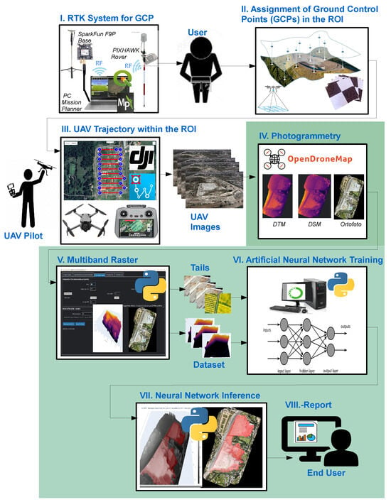
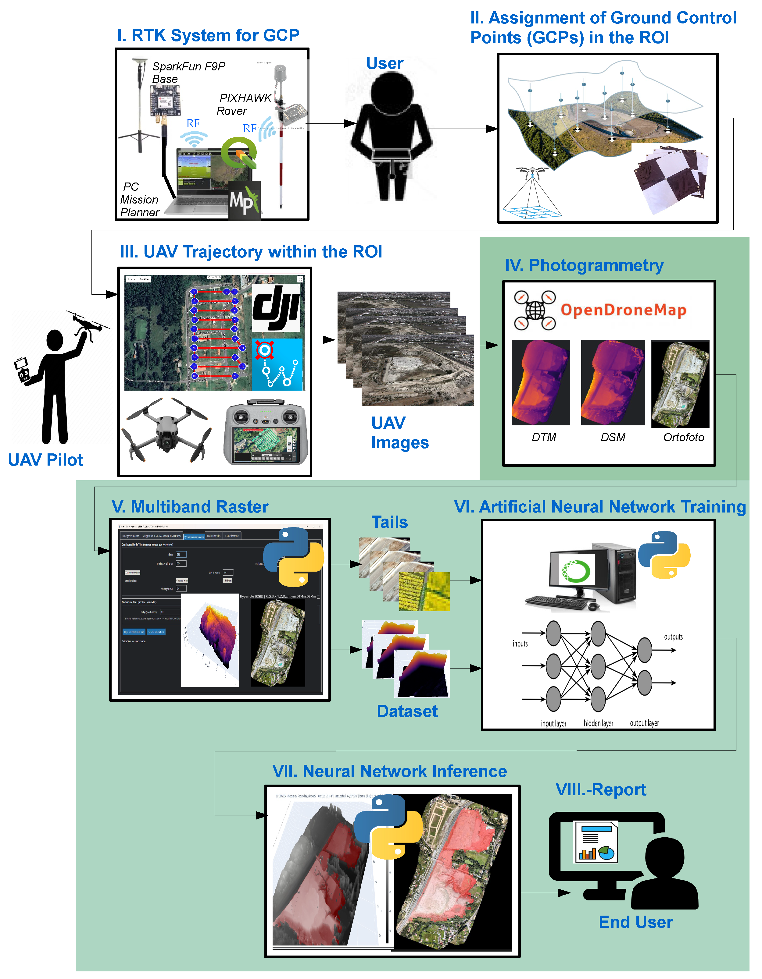
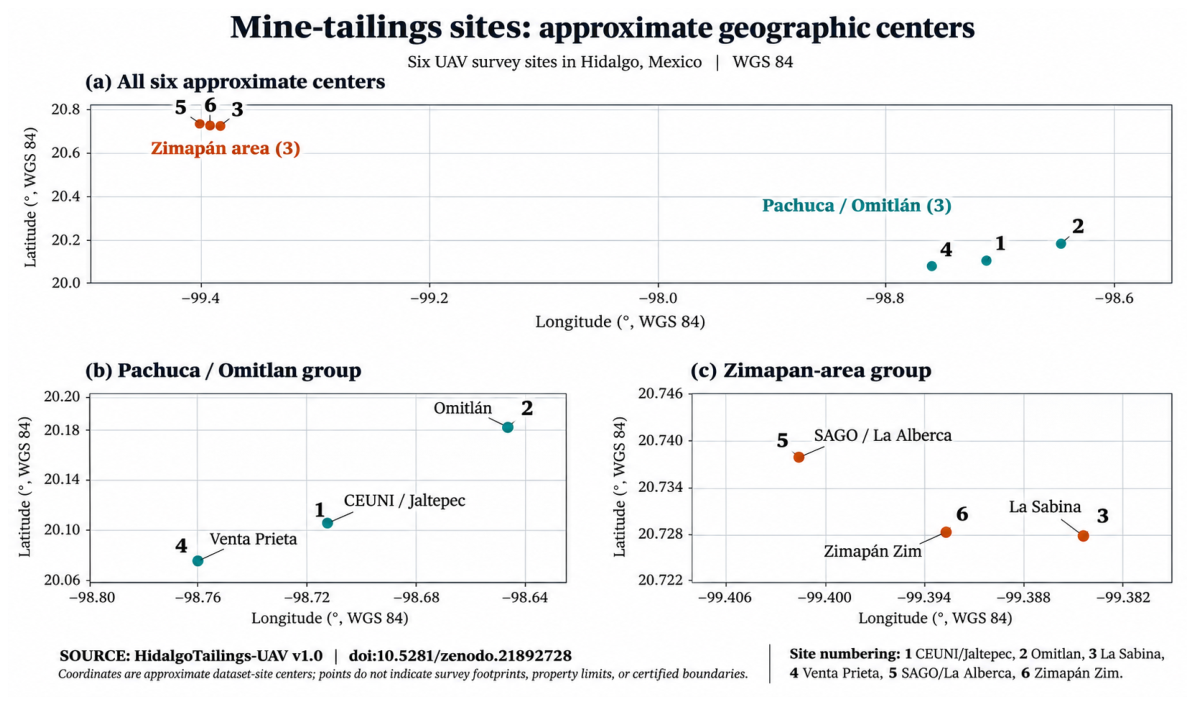
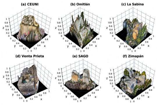
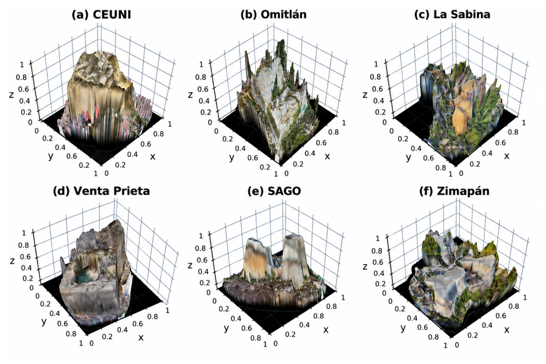
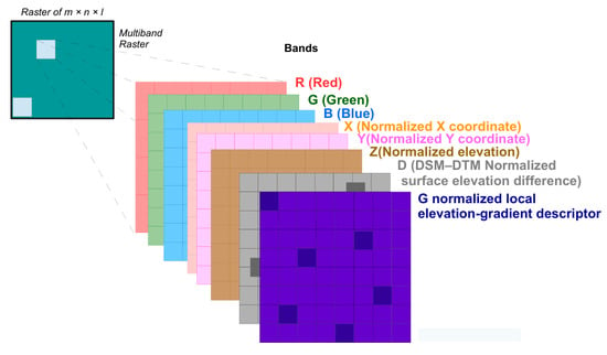
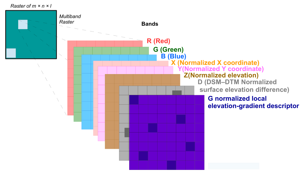
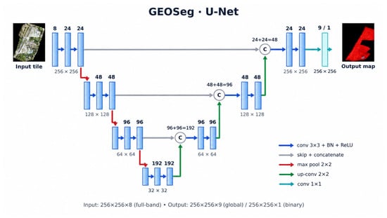
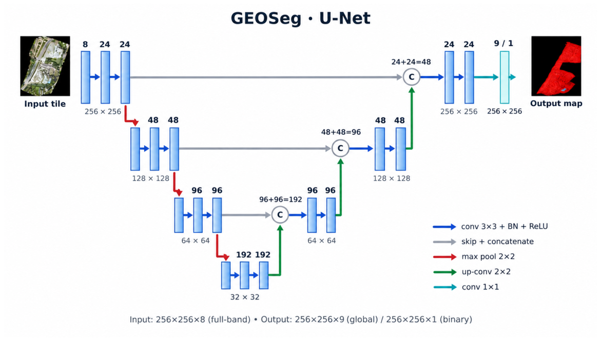
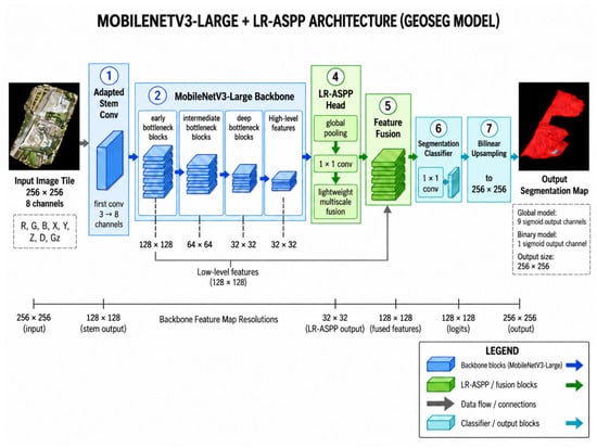
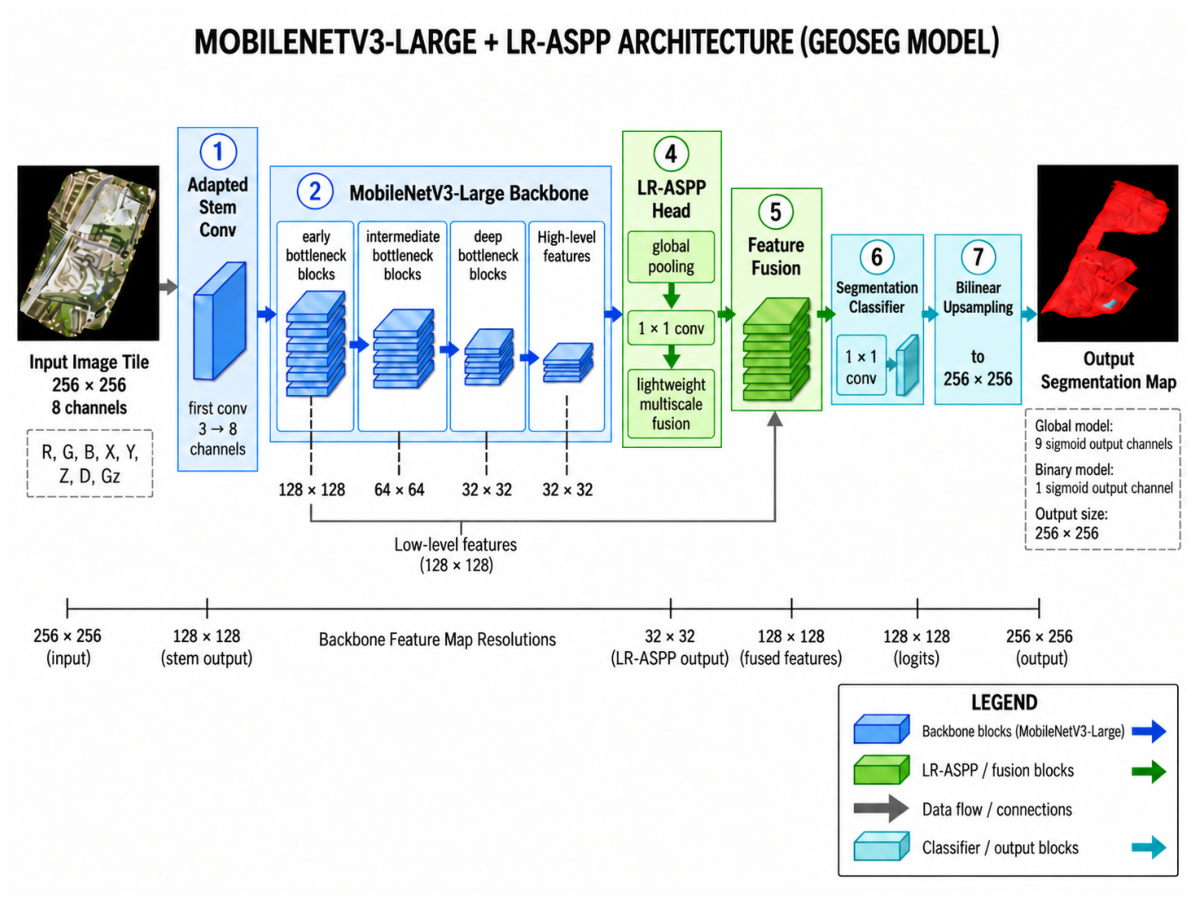
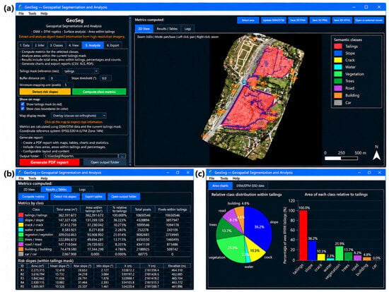
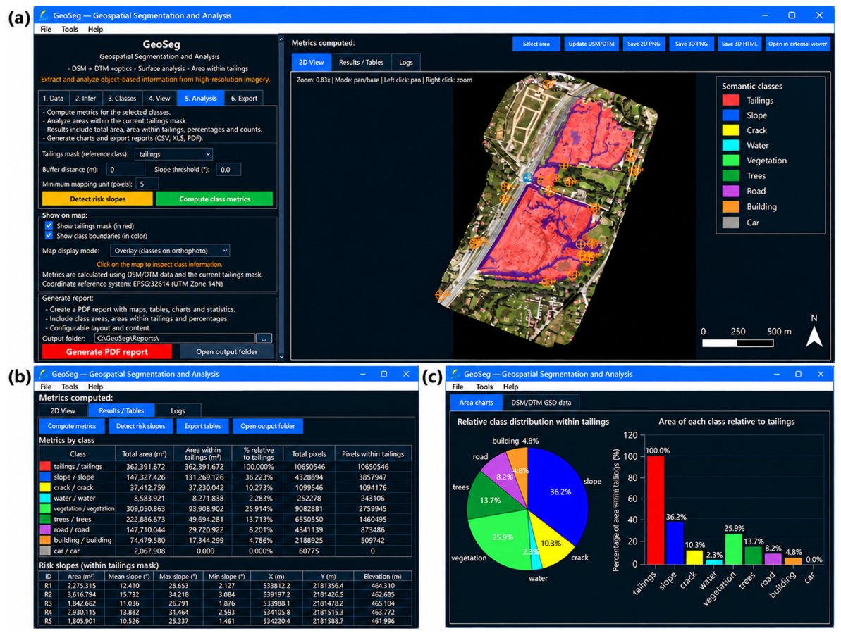
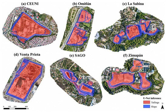
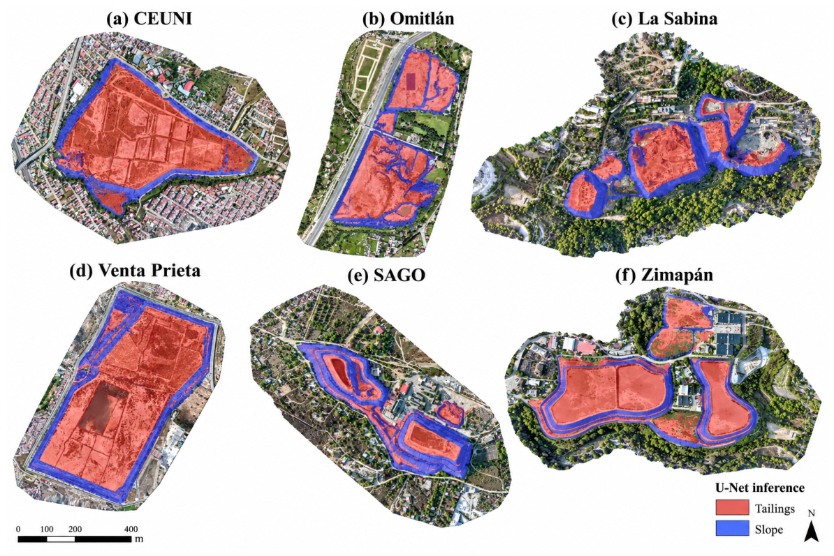

Disclaimer/Publisher’s Note: The statements, opinions and data contained in all publications are solely those of the individual author(s) and contributor(s) and not of MDPI and/or the editor(s). MDPI and/or the editor(s) disclaim responsibility for any injury to people or property resulting from any ideas, methods, instructions or products referred to in the content. |
© 2026 by the authors. Licensee MDPI, Basel, Switzerland. This article is an open access article distributed under the terms and conditions of the Creative Commons Attribution (CC BY) license.