


Abstract
In the mining industry, where equipment breakdowns cause expensive unplanned downtime, operational continuity is paramount. Internet of Things (IoT) technologies have the potential to make predictions; however, most solutions lack a holistic view and mapping of complex system interdependencies. This study presents a comprehensive predictive maintenance (PdM) framework specifically designed for continuous-operation mining environments, with a primary focus on Semi-Autogenous Grinding (SAG) mills. By combining exploratory data analysis, advanced feature engineering, classical machine learning (Gradient Boosting Classifier), and deep learning (LSTM with multiple time-window configurations), the system achieves real-time anomaly detection, root-cause explanation, and failure forecasting up to 48 h in advance (average lead time: 17 h). A four-layer digital twin architecture integrated with Streamlit enables actionable alerts classified as emergency, planned, or preventive interventions. Applied to a one-year dataset comprising 99,854 hourly records from an industrial SAG mill, the hybrid model prevented an estimated 219.5 h of unplanned downtime, yielding substantial economic benefits. The proposed solution is deliberately designed for high adaptability across multiple equipment types and industrial sectors beyond mining.
1. Introduction
The mining industry is characterized by non-stop production cycles. As a result, certain machinery and equipment in the operation continues to run non-stop throughout this process. This intense working environment accelerates equipment degradation, making maintenance a critical operational factor. Traditional maintenance processes rely on fixed maintenance intervals (preventive) or sending equipment for repair after a breakdown occurs (corrective). These traditional methods lead to high costs caused by production interruptions, part replacements, and wasted labor.
With the integration of Internet of Things (IoT) technology, real-time data storage and analysis of machines has been enabled [1,2]. There has been a shift toward condition-based monitoring. This technology increases the success rate of failure prediction by continuously monitoring parameters such as temperature, pressure, and vibration. Kruczek et al. [3] addressed the reduction in machine failures and optimization through big data analytics via IoT-based systems in their work. In this study, cloud technology reduces costs and increases efficiency thanks to the correlation between IoT and predictive maintenance [4].
The operability of system machines is affected by environmental conditions in terms of the applicability of the models produced. Recent approaches have focused on automated machine learning (AutoML) to improve fault classification under these varying conditions [5]. For example, environmental conditions such as high temperatures and dust cause machine and equipment failures [6]. Another study discusses how the model can be optimally developed under such adverse conditions [7].
Hsu et al. [8] examined the determination of the remaining useful life of equipment and machinery and its applicability in extending the life of critical equipment. Modeling was performed using machine learning and deep learning models. Dayo-Olupona et al. [1] conducted a study on the mechanics of predictive modeling. The study shows the operation of models that can be used according to the machine and equipment.
Aqueveque et al. [9] state that predictive maintenance aims to optimize maintenance processes by monitoring the operational processes of machines and equipment. This method is important to prevent significant losses resulting from production interruptions. Rihi et al. [10] emphasize in their work that the predictive maintenance system approach significantly reduces downtime. The study compares modern technology and traditional methods, highlighting the superiority of the modern method. In another study, the adaptability of neural networks, deep learning, and many other such models to the system, their approaches, and data definitions were made [11]. Another study focuses on the necessity of collecting, storing, analyzing, controlling, and reporting data for the system to operate efficiently [12].
In conclusion, studies prepared for predictive maintenance provide significant contributions in terms of supporting the effectiveness of this technology not only for fault systems but also in areas such as increasing efficiency, combating environmental impacts, and similar fields [13,14]. Predictive maintenance (PdM) stands out as a technology that can minimize unplanned downtime and costs by monitoring the operation of equipment and analyzing the data obtained through its algorithms, addressing the inefficiencies of traditional methods and leaving decision-making to artificial intelligence. However, a significant gap remains in the integration of these technologies. While individual studies address environmental constraints [6] or specific algorithmic adaptations [11], few approaches view the mining operation as a holistic system. Existing solutions often lack a ‘Systems Thinking’ perspective, failing to map the complex interdependencies between sensor data, environmental variables, and operational logic.
This study aims to bridge the gap by establishing an advanced and highly adaptable predictive maintenance system for mining operations by conducting research, developing innovative models, and creating solutions that increase efficiency. Emerging research in 2025 [15] reinforced the necessity of hybrid AI frameworks in mining, demonstrating that combining distinct algorithmic strengths is essential for handling the complex, multi-variable nature of mineral processing data. Unlike distinct algorithmic studies, this research utilizes a Systems Thinking approach to define system architecture and interdependencies. A hybrid infrastructure combining machine learning and deep learning algorithms was developed. Finally, a Streamlit-integrated digital twin architecture was created to enable real-time operation and action of the algorithms. To move beyond standard implementation and address the theoretical limitations of existing predictive maintenance models, this study investigates two specific research questions: (1) Can the integration of ‘Systems Thinking’ (MICMAC analysis) reduce the dimensionality and noise inherent in mining sensor data better than standard correlation methods? (2) Does a hybrid architecture combining classical machine learning (for feature classification) with LSTM (for temporal forecasting) outperform standalone deep learning models in environments with extreme class imbalance? The following sections detail the experimental framework designed to answer these questions.
2. Materials and Methods
2.1. Research Subject and Dataset
This research focuses on a high-capacity Semi-Autogenous Grinding (SAG) mill operating within a 24 h production cycle across three shifts. The dataset comprises one year of operational telemetry, totaling over 500 million raw sensor readings, which were aggregated into 99,854 hourly records. The research subject was monitored via 154 distinct data features, including average mill speed, pulp density, feed counter, acoustic emissions, motor power consumption, and main bearing pressure. This specific equipment was selected due to its critical role as a bottleneck in the comminution circuit and its susceptibility to complex, non-linear failure modes. Crucially, the mechanical and tribological laws governing SAG mill operations are physical constants rather than temporal trends. Therefore, the failure modes and stress correlations captured in this dataset are time-invariant, ensuring the model’s applica-bility to modern equipment reliability regardless of the data collection year.
To strengthen the foundation of the predictive maintenance system, the environment was examined in detail using Systems Thinking and analysis, and analyses were performed. The most important part of these analyses involves interpreting the results. A modeling framework was developed using the outputs of Systems Thinking and analysis, which determined the parameters selected during development of the predictive maintenance algorithm.
2.2. Systems Thinking and MICMAC
To understand the complex causal relationships within the maintenance ecosystem, the MICMAC method was employed. This analysis identified parameters with the strongest influence–dependence relationships, categorizing variables into influential, key, dependent, and excluded sectors. The result of this analysis dictated to the system, in terms of algorithm selection, which sensors should be used for modeling, elements to be considered in the analysis of data obtained from sensors, and similar situations.
The key parameters identified for the system included sensors, data collection system, cloud storage, machine learning models, data analysis platform, real-time monitoring panels, warning system, maintenance planning module, control center operator, maintenance unit, and IT.
2.3. Sensor Network and Data Acquisition
The input layer of the proposed system consists of a sensor network installed on a Semi-Autogenous Grinding (SAG) mill. The accuracy of the predictive algorithms is directly correlated with the positioning and fidelity of these sensors. The instrumentation profile includes sensors for motor power, bearing pressure, vibration, acoustic emission (sound), feed flow rate, and material density.
2.4. Data Collection Frequency
Data transmission rates were calibrated based on the dynamic nature of the monitored variables. Slow-varying parameters, such as bearing pressure, were sampled at 1 Hz. However, high-frequency variables, particularly acoustic emissions, required significantly higher sampling rates. Adhering to the Nyquist–Shannon Sampling Theorem, the sampling frequency (fs) was set such that
where fmax represents the highest frequency component of the signal, ensuring no aliasing occurred during data capture.
fs ≥ 2 · fmax
2.5. Data Preprocessing and Storage Architecture
The data obtained from sensors must first undergo preprocessing and analysis, and an algorithm must be developed based on this data.
A dual-format storage strategy was implemented to balance immediate accessibility with long-term archival efficiency.
- Data Ingestion: Raw sensor data is initially processed in Comma-Separated Values (CSV) format to ensure compatibility with standard preprocessing libraries.
- Archival: To manage the volume of the data, daily CSV logs are converted to Apache Parquet format. Parquet is a columnar storage file format that provides significant compression and efficient data retrieval. This allows the system to query specific columns (e.g., only ‘Motor power’) without scanning the entire dataset, significantly reducing input/output overhead costs.
2.6. Real-Time Data Transmission via MQTT
After developing the algorithm, the next step involves creating a Streamlit-based (Version 1.43.0) interface. Due to insufficient capabilities of the underlying software libraries to provide real-time data, a messaging protocol Message Queuing Telemetry Transport (MQTT) was implemented for instantaneous data transmission.
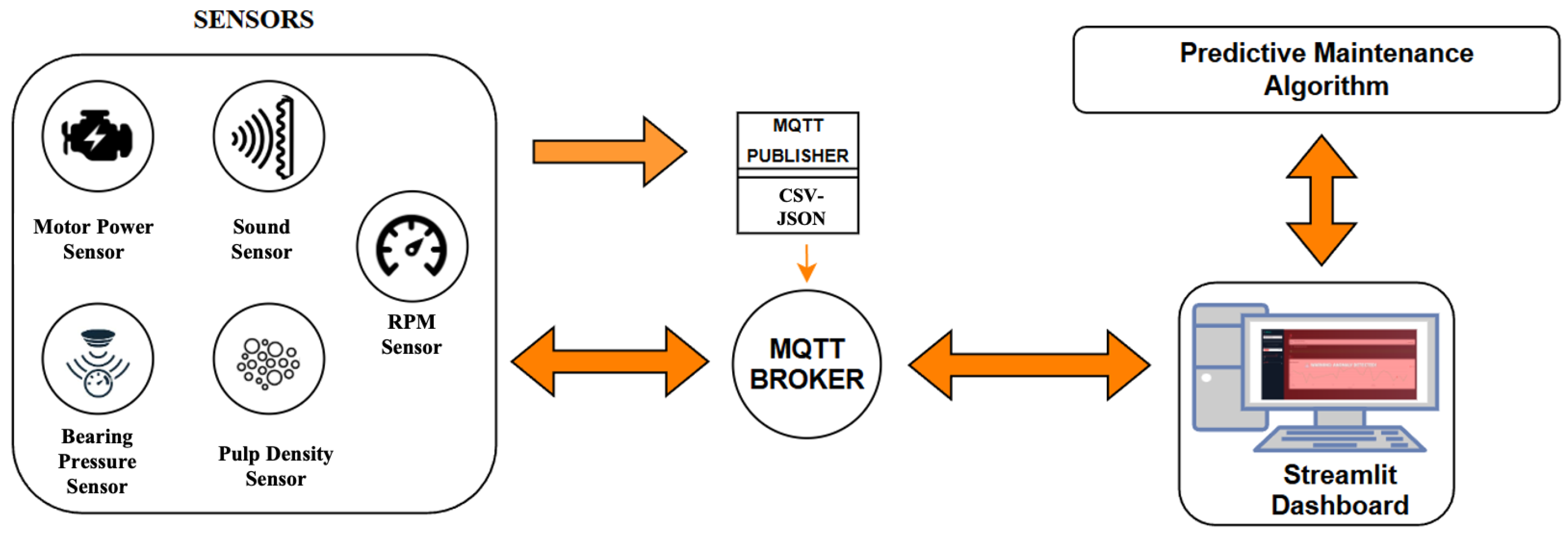
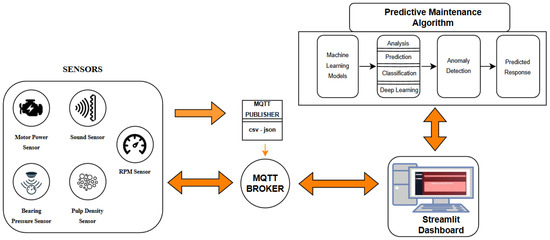
MQTT, one of the data transmission approaches, is a subscription protocol between sensors and analysis platforms. According to this system, a central proxy server receives messages from sensors in JSON format and provides instant updates to the Streamlit interface acting as a client through a subscription (see Figure 1). This system, which transmits data in real time, eliminates data latency. Furthermore, slowdowns in the system caused by large amounts of data can be prevented thanks to this system. On the other hand, it holds incoming messages in intermittent network conditions and performs the necessary updates on the client.
Figure 1.
The role of MQTT communication in the system.
3. Results
Effective predictive maintenance relies on a sequential pipeline of data discovery, data cleaning, feature engineering, and data modeling. Rather than following a rigid roadmap, an iterative approach was adopted where the output of each stage informed the strategy for the next. This section details the application of this pipeline to the SAG mill dataset.
The data must first be examined and analyzed with exploratory data analysis, and unnecessary data must be cleaned as a result of the discoveries made. Then, feature engineering must be performed to establish connections between the data and form the basis for modeling, and finally, the model must be trained. Decisions and strategies should be determined at the end of each stage. Because each stage has its own methods, the outputs they provide may be specific to the analyzed data. Therefore, instead of drawing a roadmap at the outset, creating new rotations at the end of each stage can ensure the reality and permanence of the system to be established.
3.1. Exploratory Data Analysis and Data Cleaning
The first step in developing the algorithm is to examine the existing data. A comprehensive review of the data collected from the sensors will identify missing values, anomalies, and features that can be used during model development.
During the data examination, zero values were observed for some records. These values were generally observed in the sound and motor power data. Under normal conditions, situations such as a mill operating without making any noise or operating at zero speed would not be observed. Therefore, when developing the model, it is necessary to exclude these data so that the machine does not perceive these situations as anomalies and does not make unrealistic detection errors. For this reason, periods containing zero values have been filtered out.
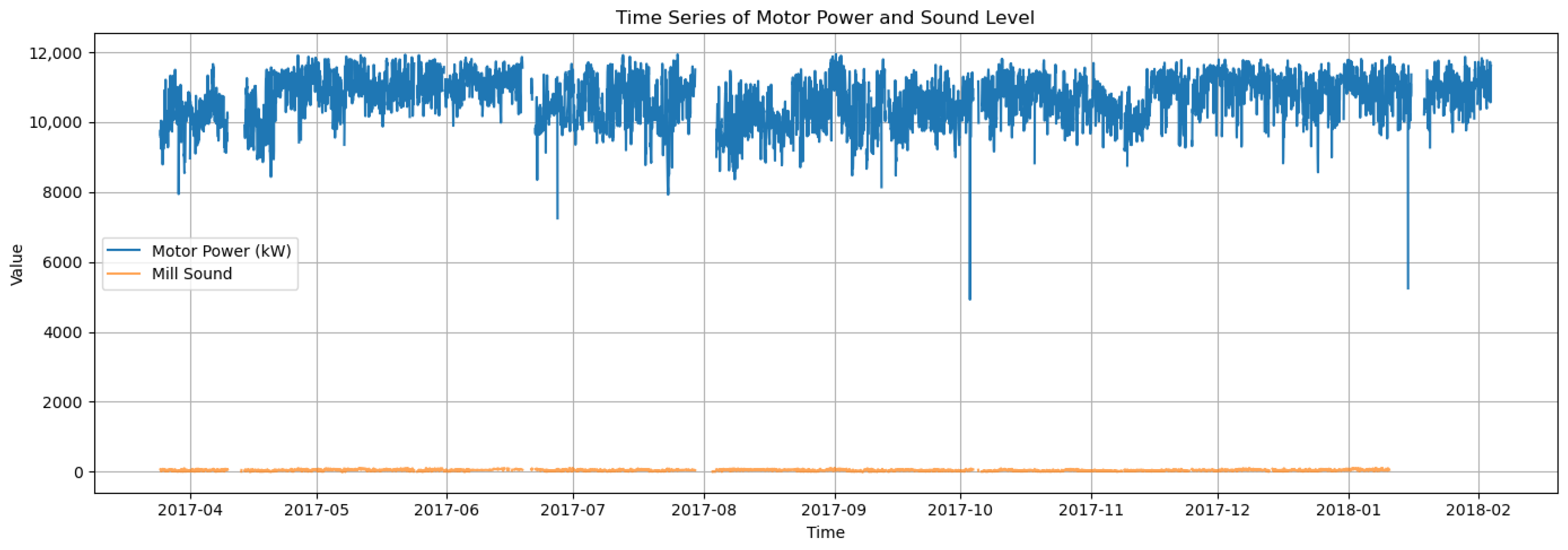
When sound and motor power are examined together in the time series, it is observed that motor power and sound level produce data in parallel (see Figure 2). This parallel relationship indicates that when the load increases, the motor consumes more power and the resulting impacts also increase. This situation is anticipated to be critical data in terms of increasing both energy and acoustic pressure in the mill, and it is supported by other analyses.
Figure 2.
Hourly distribution of motor power and noise data in the time series.
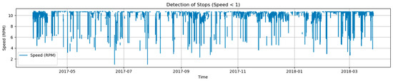
When examining the speed data in Figure 3, based on the time series, if the speed is less than one revolution per minute, the mill may be stopped or undergoing maintenance. In this case, speeds of 1 RPM (revolutions per minute) or less have been filtered to prevent the model from directly identifying them as anomalies.
Figure 3.
Change in mill speed over time.
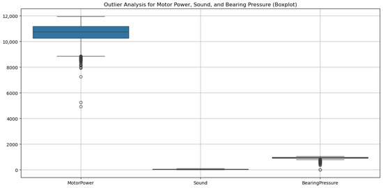
An outlier analysis was performed for motor power, noise level, and bearing pressure, as shown in Figure 4. According to this analysis, situations with high variance should be investigated as they may indicate a malfunction. Based on this output, bearing pressure was very low at certain times. This situation indicates that the data quality of the sensors needs to be updated or that quality control needs to be repeated. Outliers in sound and motor power, on the other hand, indicate the possibility of pre-malfunction situations.
Figure 4.
Outlier analysis for motor power, noise, and bearing pressure.
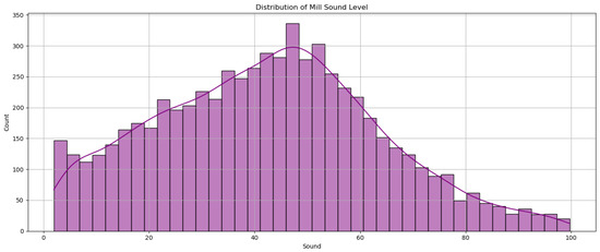
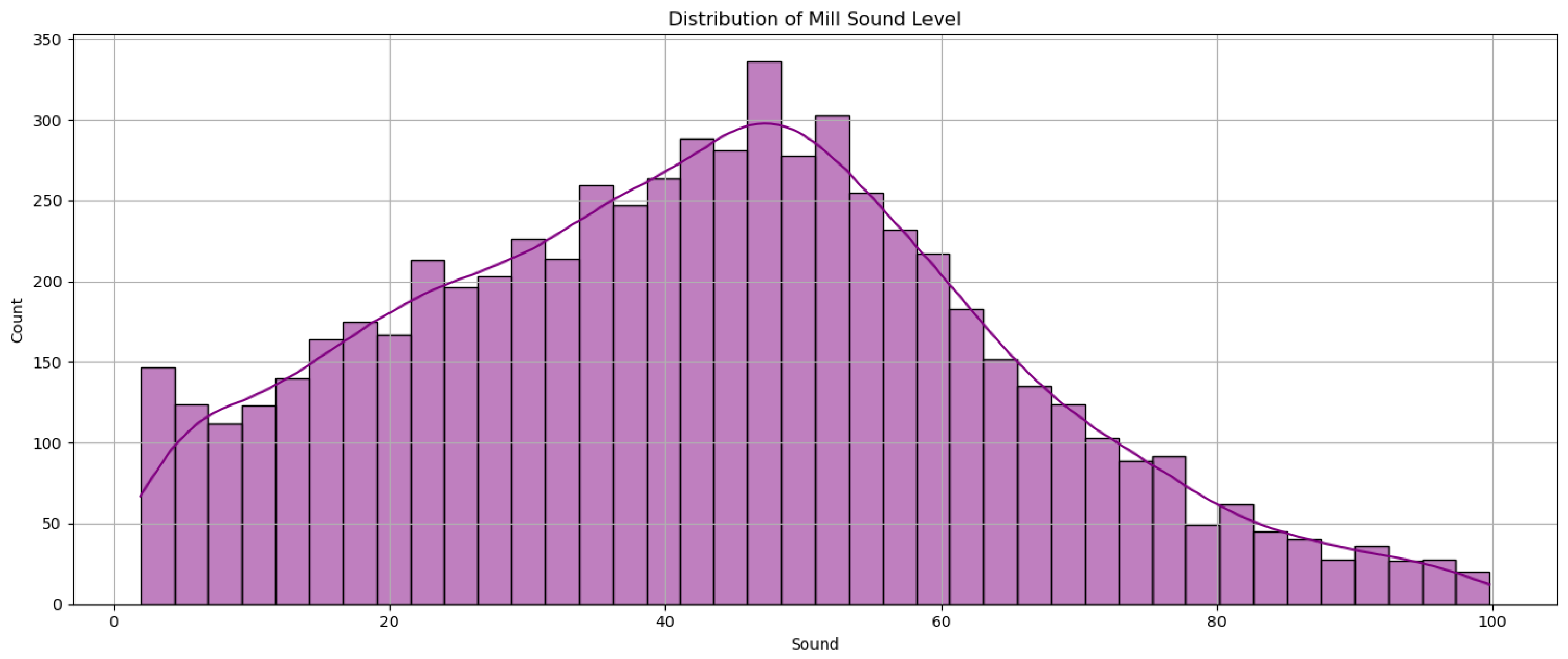
Figure 5 represent sound level frequency distribution with trend line. When the noise level of the mill is examined as a normal distribution as shown in Figure 5, it is observed that it is not consistent with the normal distribution. In this case, skewness becomes apparent. The right skewness of the distribution highlights the criticality of sounds originating from sudden impact events. This situation will facilitate the algorithm’s ability to distinguish anomalies and increase the success rate.
Figure 5.
Normal distribution of sound levels.
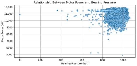
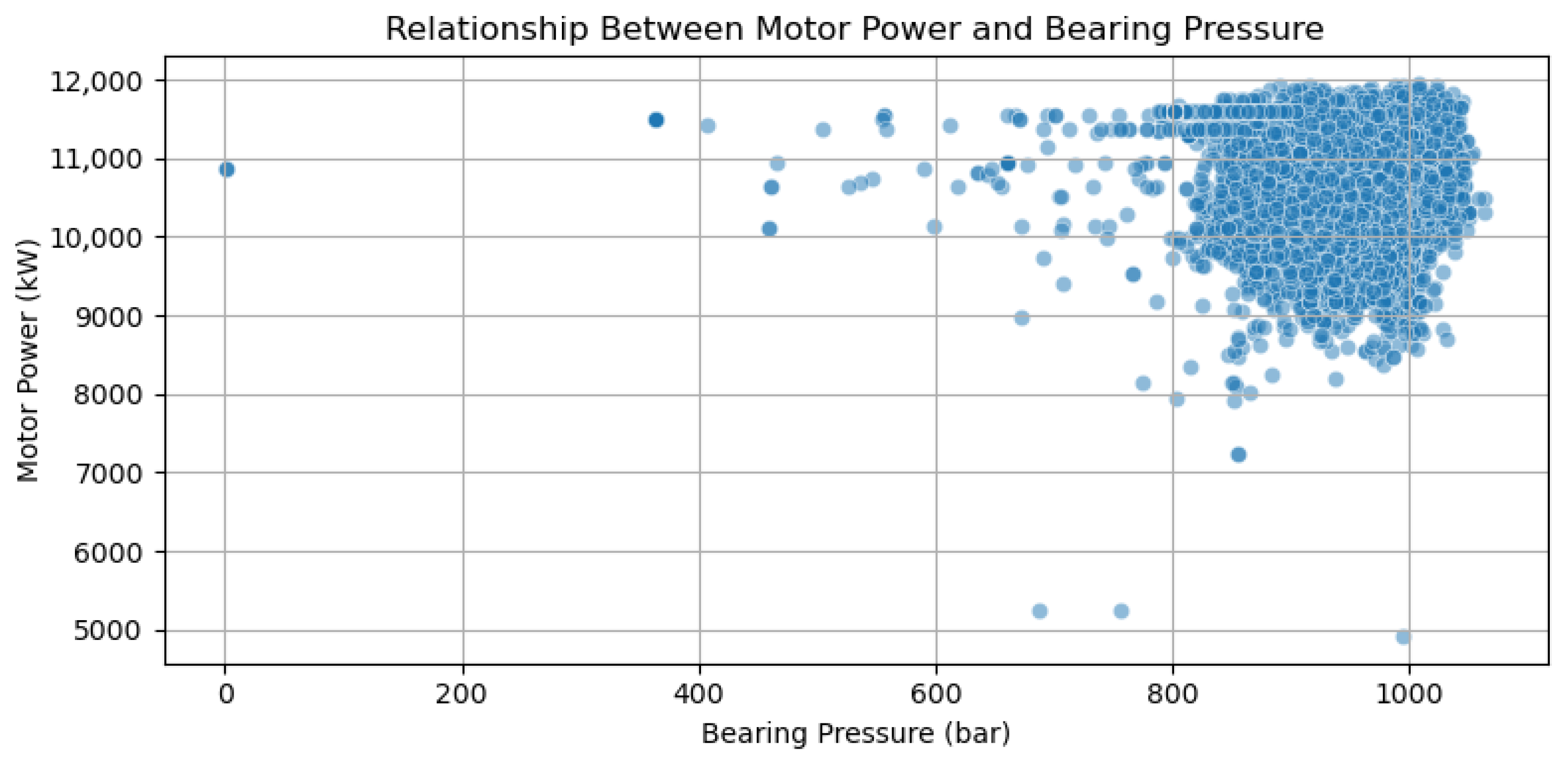
The relationship between motor power and bearing pressure is examined in Figure 6, revealing a positive correlation between them. This correlation indicates that both mechanical pressure and energy consumption increase as the load increases. At certain points, however, the motor power is high while the bearing pressure is low. This situation represents energy waste for the system. Since these two indices can produce multiple different results, a stress index can be introduced. This can be beneficial in terms of introducing a new column for feature engineering to the data set. The product of these two indices yields the stress index. This index reveals the amount of internal stress on the mill. This makes it possible to comment on the energy expended as a result of this stress. By analyzing the energy expanded by the mill under load, it was possible to determine whether a mechanical stress condition has occurred. This analysis provides insight into potential damage.
Figure 6.
Distribution graph showing the relationship between motor power and bearing pressure.
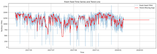
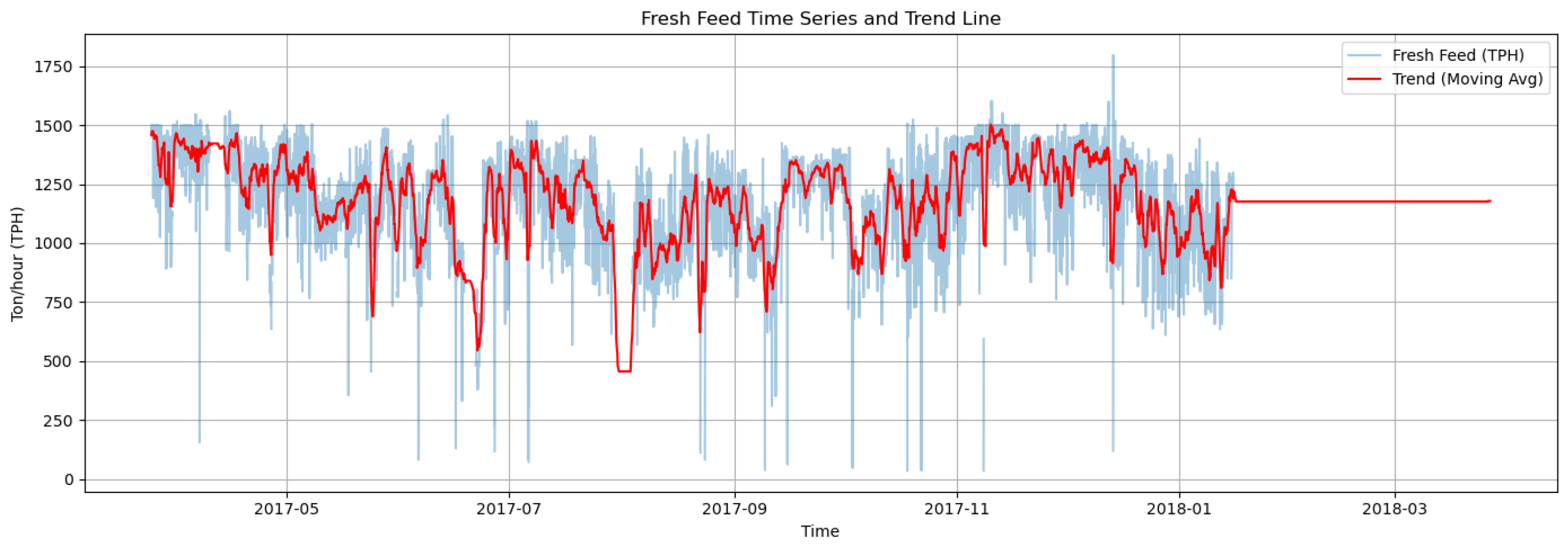
When examining the moving average trend of fresh ore feed data, it is observed that the system’s feed rate follows a normal pattern, but sudden changes occur at certain points (see Figure 7). Considering that this situation may be due to material being drawn from stock instead of the crusher or post-failure conditions, it has been cleaned so that the model does not perceive it as an anomaly.
Figure 7.
Behavior of fresh ore feed data on the trend line.
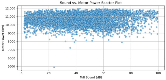
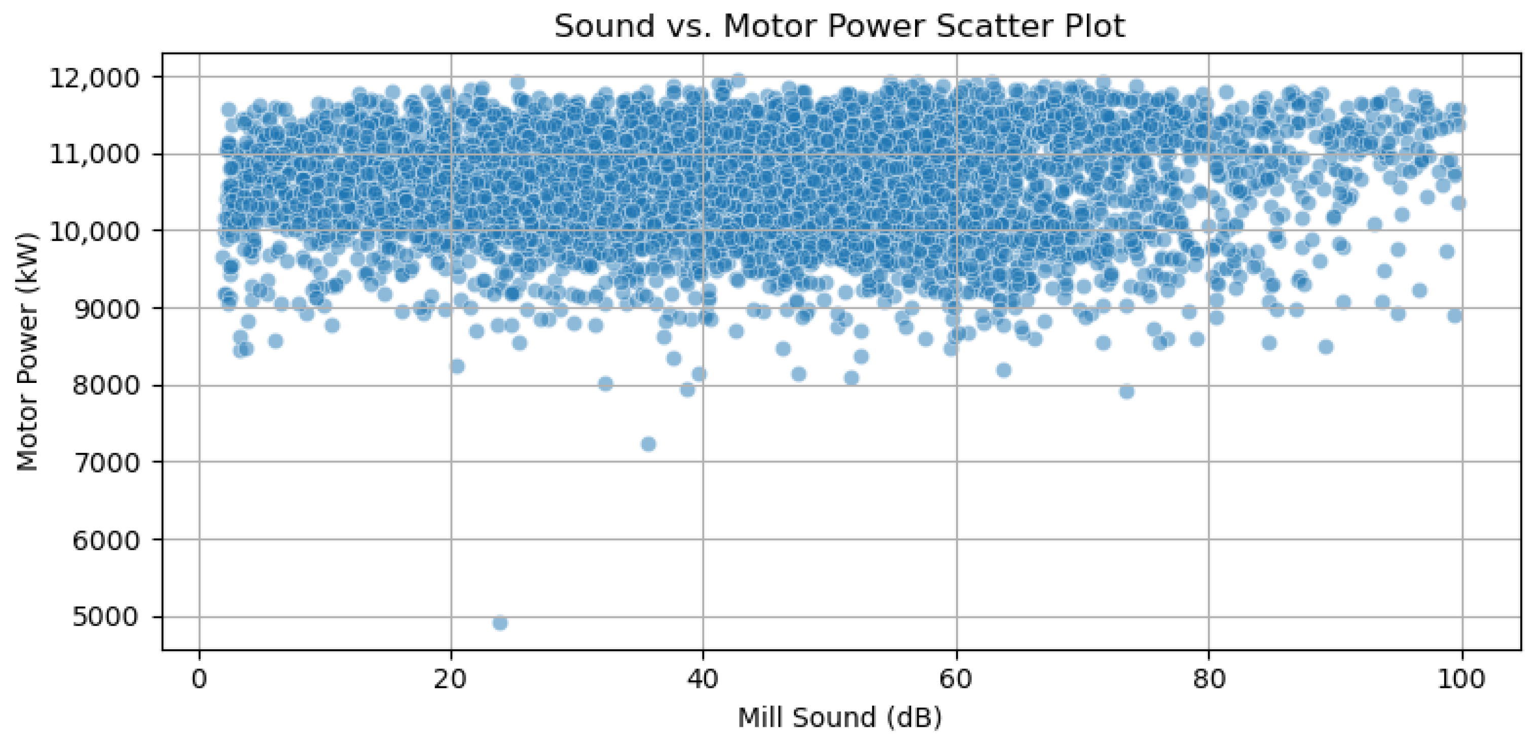
When examining the relationship between sound data and motor power data in the distribution graph, it is observed that as power increases, sound also increases (see Figure 8). However, this correlation shows a moderate level of correlation rather than a high level of correlation. The most important part of this output is the occurrence of low sound levels at very high motor power or the detection of high sound data at low motor power levels. This situation may be caused by idle collisions or sensor shifts. For this reason, the model has been cleaned to prevent incorrect prediction and classification. Furthermore, this output shows that the sound data is sensitive to anomalies. Due to this sensitivity to anomalies, it was deemed appropriate to use sound data in the examination of the data prior to developing the model.
Figure 8.
Distribution graph of the correlation between motor power and noise data.
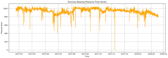
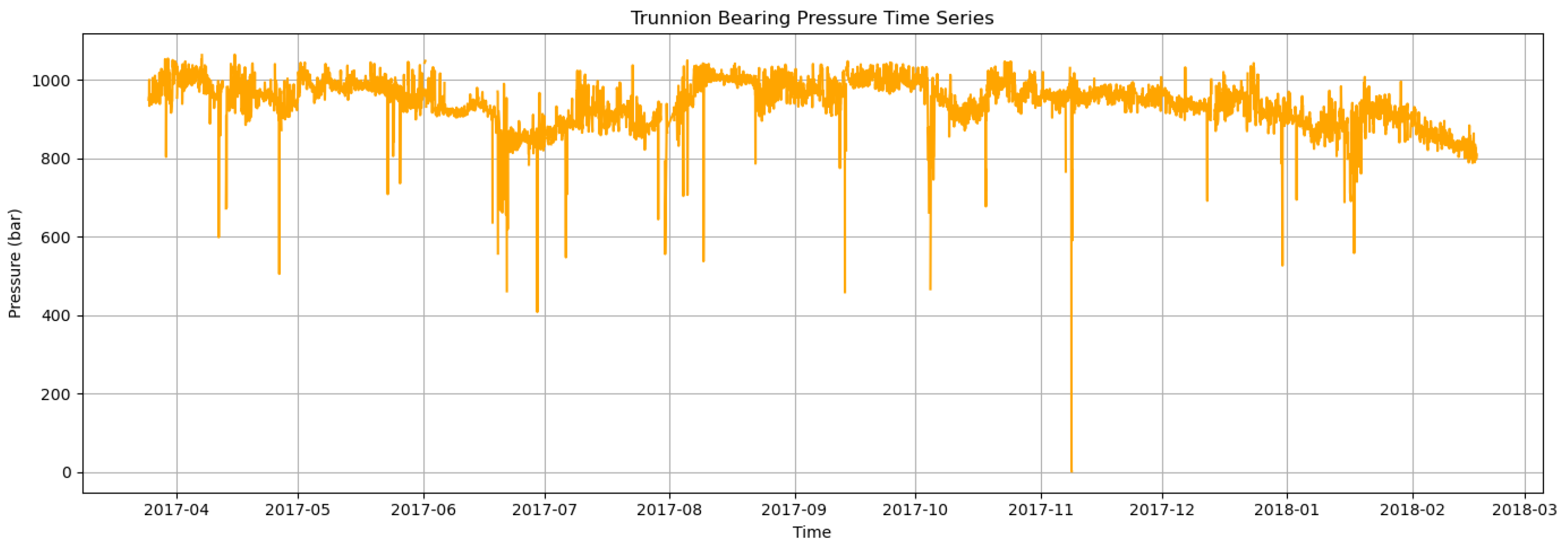
The change in bearing pressure over time, as examined in Figure 9, generally ranges between 900 and 1050 bar. However, sudden drops in pressure are observed at certain times. Although the first step was to remove empty data from the system, this situation may still be observed due to oil shortages or pump interruptions. Such situations will increase friction due to insufficient oil. This will cause wear and tear and result in extra maintenance costs. Based on this analysis, a lower pressure limit should be determined, and the system should be integrated to issue a warning if this limit is exceeded.
Figure 9.
Time-dependent change in bearing pressure data.
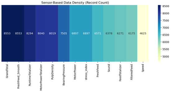
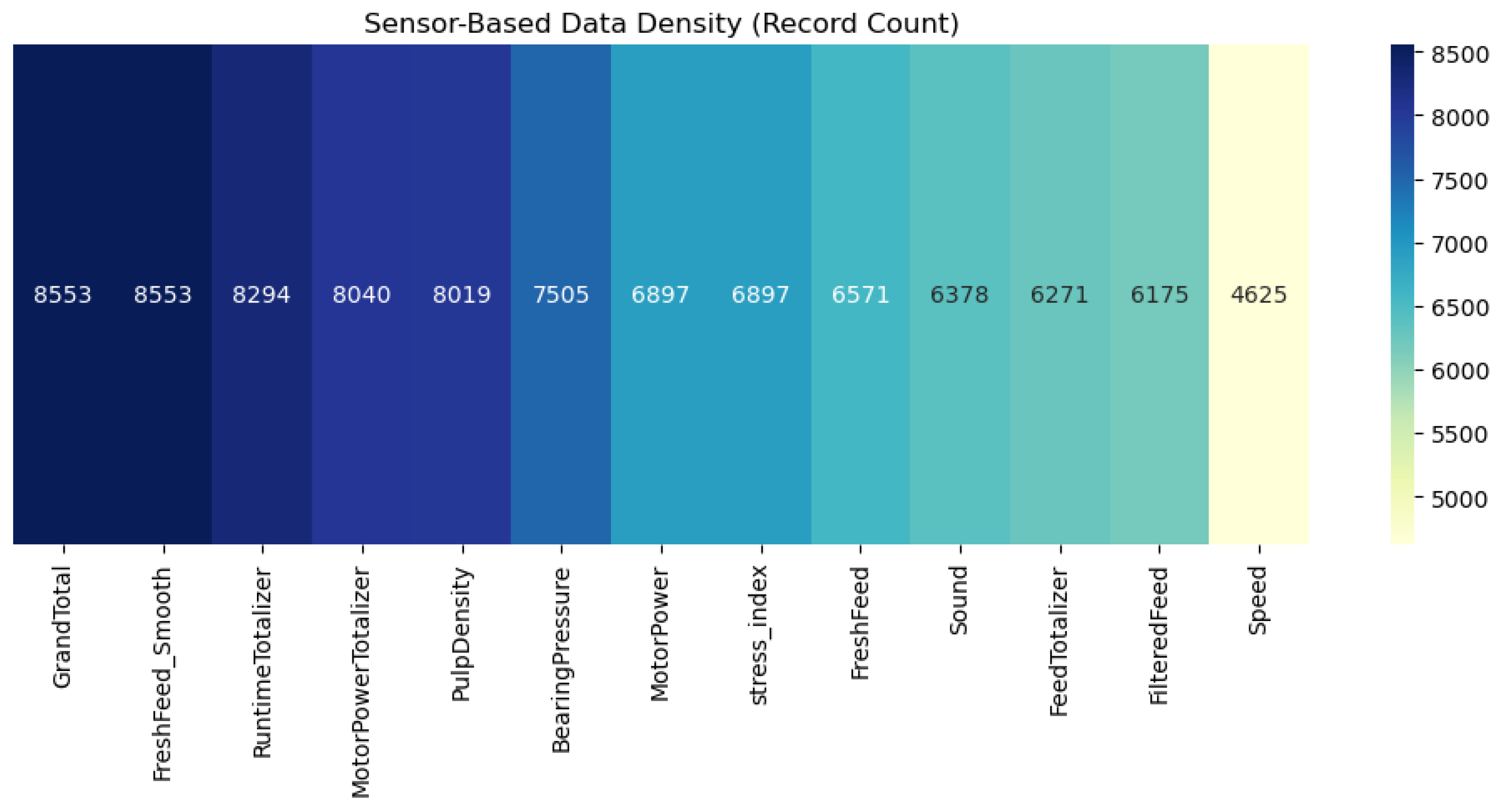
The data remaining after all cleanups are shown in Figure 10. According to this output, the sensor with the most data loss is the speed sensor. These data losses indicate that some sensors are failing more frequently. As a result, the sensor-based scoring system was able to incorporate the sensor’s confidence level into the model and, consequently, perform the prediction process.
Figure 10.
Number of data points collected from sensors after data cleaning.
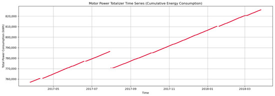
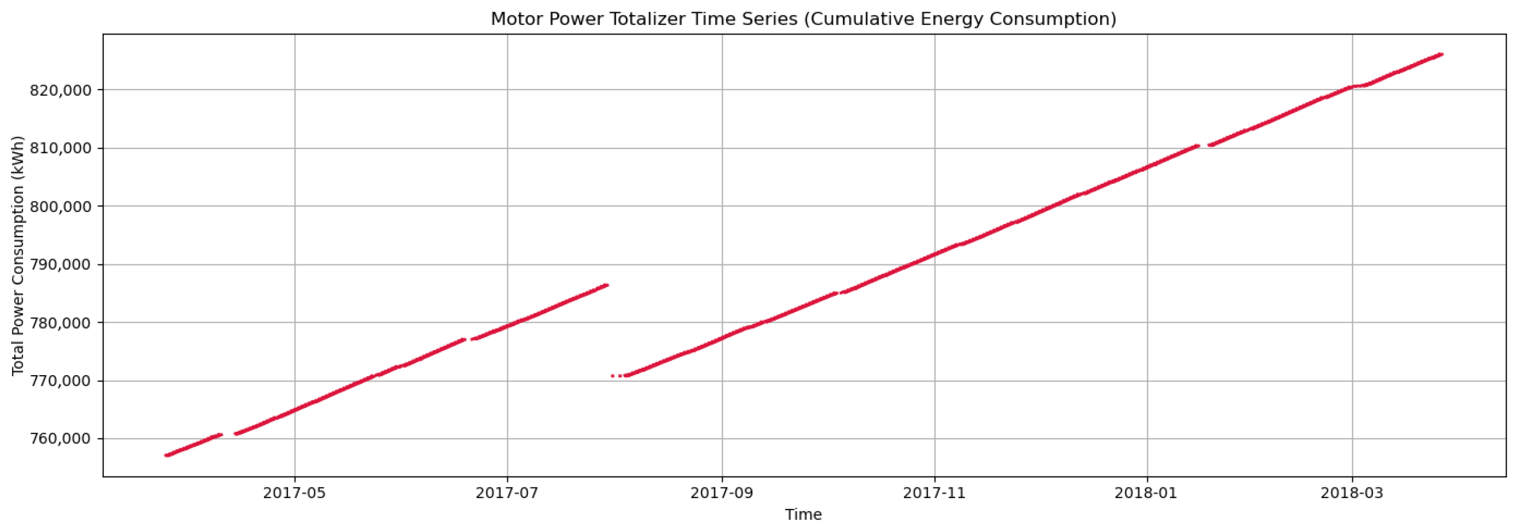
When examining the change in total power consumption over time, a generally linear increase is observed, and in the 8th month an adjustment was made to the totalizer (see Figure 11). However, sudden spikes are seen at certain times. These sudden spikes may be due to momentary overload or material jams. In this case, the energy consumption trend was derived by taking hourly differences. To develop a sudden surge alarm based on these differences, the average of the hourly energy differences was taken. For fluctuations in energy consumption, the standard deviation of the hourly differences was taken as twice the standard deviation in order to detect abnormal situations. In other words, this calculation was performed to detect situations that exceeded the 95% confidence interval. The values of this calculation, whether abnormal or not, were added to the pre-model system as an energy spike column.
Figure 11.
Change in cumulative energy consumption over time.
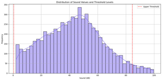
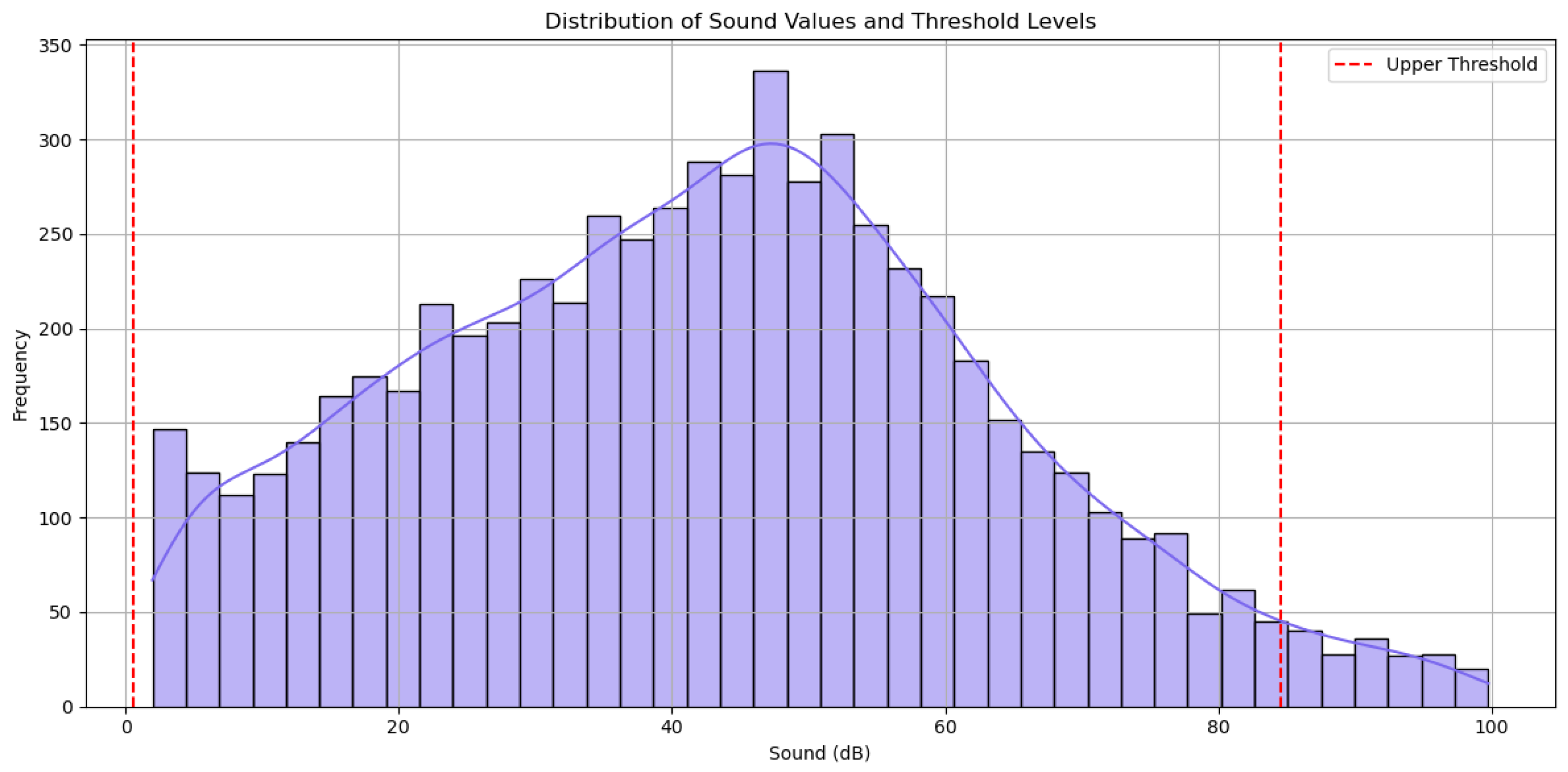
Figure 12 represent sound level frequency distribution, trend line and threshold levels. As with energy consumption, values exceeding twice the standard deviation are considered abnormal operation for the purpose of detecting sound anomalies. The lines in the normal distribution graph shown in Figure 12 represent the differences between twice the standard deviation and the mean. The areas outside these lines indicate anomalies.
Figure 12.
Distribution of sound data and threshold values.
3.2. Feature Engineering
Feature engineering was performed to enhance model stability and prediction accuracy. This process involved creating derived attributes, encoding categorical data, and addressing missing values to better represent the operational state of the SAG mill.
Some results obtained during exploratory data analysis indicated that new columns needed to be created. Based on these results, the limits for speed, valid data masks, and outlier sound values were determined. Additionally, missing values were deleted or filled with appropriate correlations. Following these cleaning steps, the idea of creating a stress index based on the relationship between motor power and bearing pressure was proposed.
The stress index represents the mechanical load and stress level in the system as a result of the product of motor power and bearing pressure. An increase in either of these two data columns can increase the stress condition. It can also alert the system about moments when strain occurs in the parts of machines operating under load. This is used in fault prediction, anomaly detection, and maintenance planning.
Thanks to the method developed by taking the absolute values of the differences between consecutive values to detect sudden changes in sound level, sudden sound changes, vibrations, loosening, cracking, impact, etc., can be detected. This is used in sudden failure detection and impact analysis.
For cumulative energy consumption, a method has been developed that makes decisions based on the difference between consecutive values to identify sudden increases and decreases. This method can enable the detection of material jams, sudden loading, or idle operation conditions. This is used in the detection of energy anomalies and efficiency analysis.
Based on the correlation between fresh feed and pulp density, the normalized feed amount according to density has been determined. Considering that excessive feeding when pulp density is low causes blockages in the system, this is used in the process stability monitoring of the feed adjustment algorithm.
The feed efficiency has been determined based on the amount of feed per unit of power. If the result of this situation is low, it can be predicted that the system is inefficient. This is important in terms of energy efficiency and system optimization.
3.3. Establishing the Basis for Anomaly Detection
In order for the machine system to be able to identify unusual data flows, deviations in the data were labeled as anomalies using an unsupervised learning approach based on the Isolation Forest Algorithm. This labeling process focused not only on the result but also on the causes. The cause system not only predicts an anomaly but also states why it will occur, facilitating the planning of the prediction system. It correlates the condition of excessively high motor power with other variables and provides a recommendation as a result. It utilizes newly created data frames to send a cooling control warning when matched with thermal overload. Similarly, it will use sound differences to match with internal impact maintenance type and generate an internal coating control warning. If the feed efficiency is low, it will match with one of the reasons, such as material blockage, and issue a feed inlet control warning. Additionally, it will detect low bearing pressure, match it with bearing clearance, and issue an oil shortage or mechanical loosening warning. In cases where no matching occurs, it will perform an unknown matching.
The warnings are based on the Local Outlier Factor algorithm. This algorithm works by classifying data based on nearby data using the nearest-neighbor model. In the established system, every 20 data points were examined, and matching was performed in cases of 5% outlier. As a result of this matching, a value of 1 is assigned for anomalies and a value of 0 for normal conditions. The reason for choosing this algorithm is that systemic failures appear as local anomalies rather than in the general distribution. Thanks to local anomaly detection, deviations that could be overlooked or undetectable can be identified.
The causes of the warning were explained using Root Cause Analysis. This removed the anomaly from being a black box and turned it into a mechanism explained by cause-and-effect relationships. This will enable more reliable maintenance planning, more accurate interpretation of error causes, and improvements in operator decisions. Unlike static quality tools such as FMEA, this system employs dynamic Root Cause Analysis to correlate real-time deviations with specific mechanical causes. This integration transforms static risk assessment into an active, predictive decision-support mechanism.
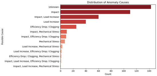
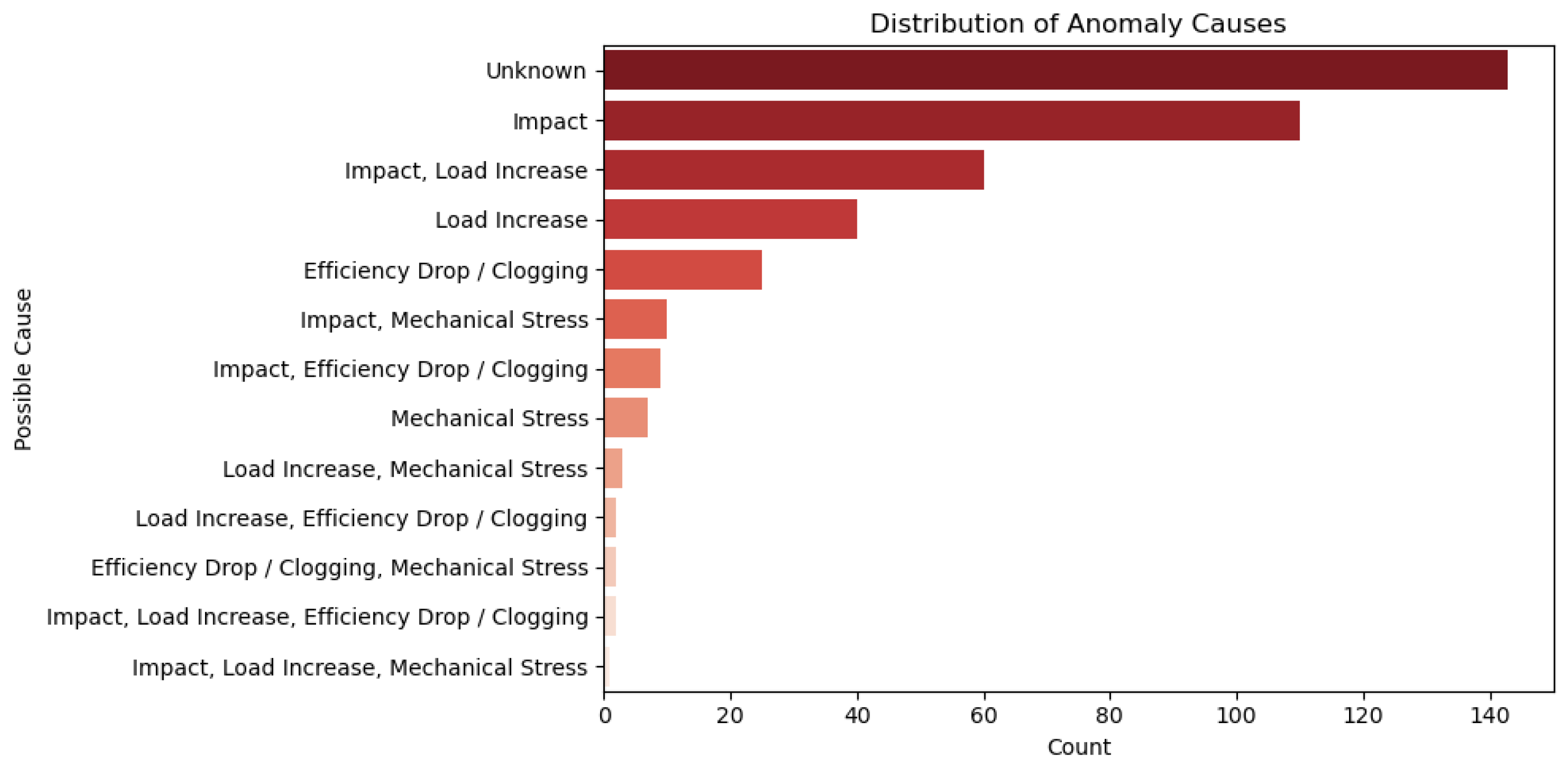
After the basic formation process, the results obtained are examined in Figure 13, where nearly 30% of the data is labeled as unknown. This situation indicates that the model detects a difference but does not match the definitions. They are matched as abnormal hours but do not exceed the value thresholds. These hours provide an ideal environment for creating new labels. The most frequent matching observed subsequently is due to impact. This indicates that collisions and material failures occur frequently within the system. This situation is followed by matches caused by load increases and mechanical stress. Integrating these high-risk situations into the system will significantly increase production efficiency.
Figure 13.
Distribution of anomaly causes.
When the 143 h of data matched as an unknown anomaly were statistically analyzed (see Table 1 and Table 2), it was observed that the motor power operated at an average of 9735 kW, i.e., under high load, the sound data operated at a medium level with an average of 46 dB, the bearing pressure operated at a normal level below the threshold at 923 bar, the stress index was under intense mechanical load, the sound threshold was below the threshold, the energy difference followed a negative trend, and the feed efficiency was low. Although the decrease in energy consumption and normal sound data during these hours may appear to indicate normal operation, it suggests that the system is approaching its efficiency and endurance limits, indicating a pre-critical stress condition. A specific label has been assigned to these hours, defining the new system as normal, anomaly, and hidden anomaly. This will enable the implementation of an early warning system.
Table 1.
Statistical values of unpaired data.
Table 2.
Continuation of statistical values for unknown matched data.
3.4. Development of the Anomaly Detection System
When establishing the anomaly detection foundation, the data matched and analyzed as unknown resulted in three types of anomaly assignments. According to this matching system, data within the threshold values are matched as normal, while abnormal situations outside the threshold are matched as anomalies. Values outside these situations, i.e., those within the threshold values but behaving abnormally, are matched as unknown. This situation has played an active role in the development of the early warning system.
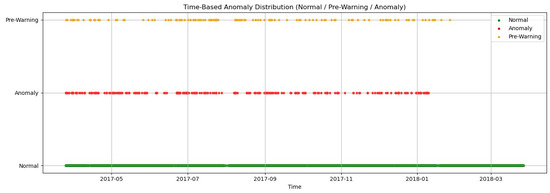
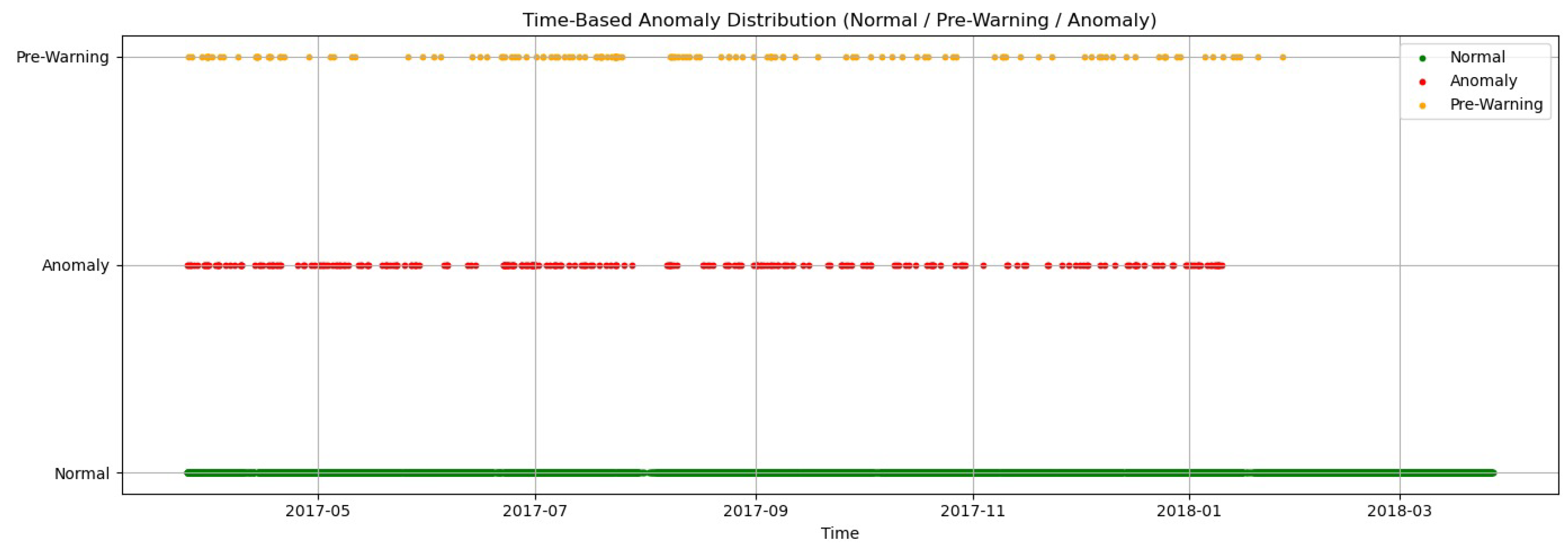
Values matched as unknown were matched as early warnings. The distribution graph of normal, anomaly, and early warning data over time is shown in Figure 14. According to this Figure, there were frequent early warnings between April 2017 and June 2017. Anomalies were observed immediately after these early warnings. This situation indicates that the system is approaching failure but also that the warnings are effective. When examining the period between July and August of this year, it is seen that early warnings have become less frequent. This indicates that maintenance has been performed or that the system has temporarily stabilized. Later, when examining the period between September and December 2017, it is observed that the early warning came first, followed by the actual anomaly occurring within 5–10 h without delay. This system behavior is consistent with the Long Short-Term Memory (LSTM) working mechanism.
Figure 14.
Anomaly distribution graph over time.
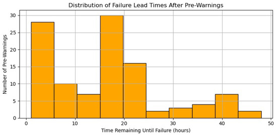
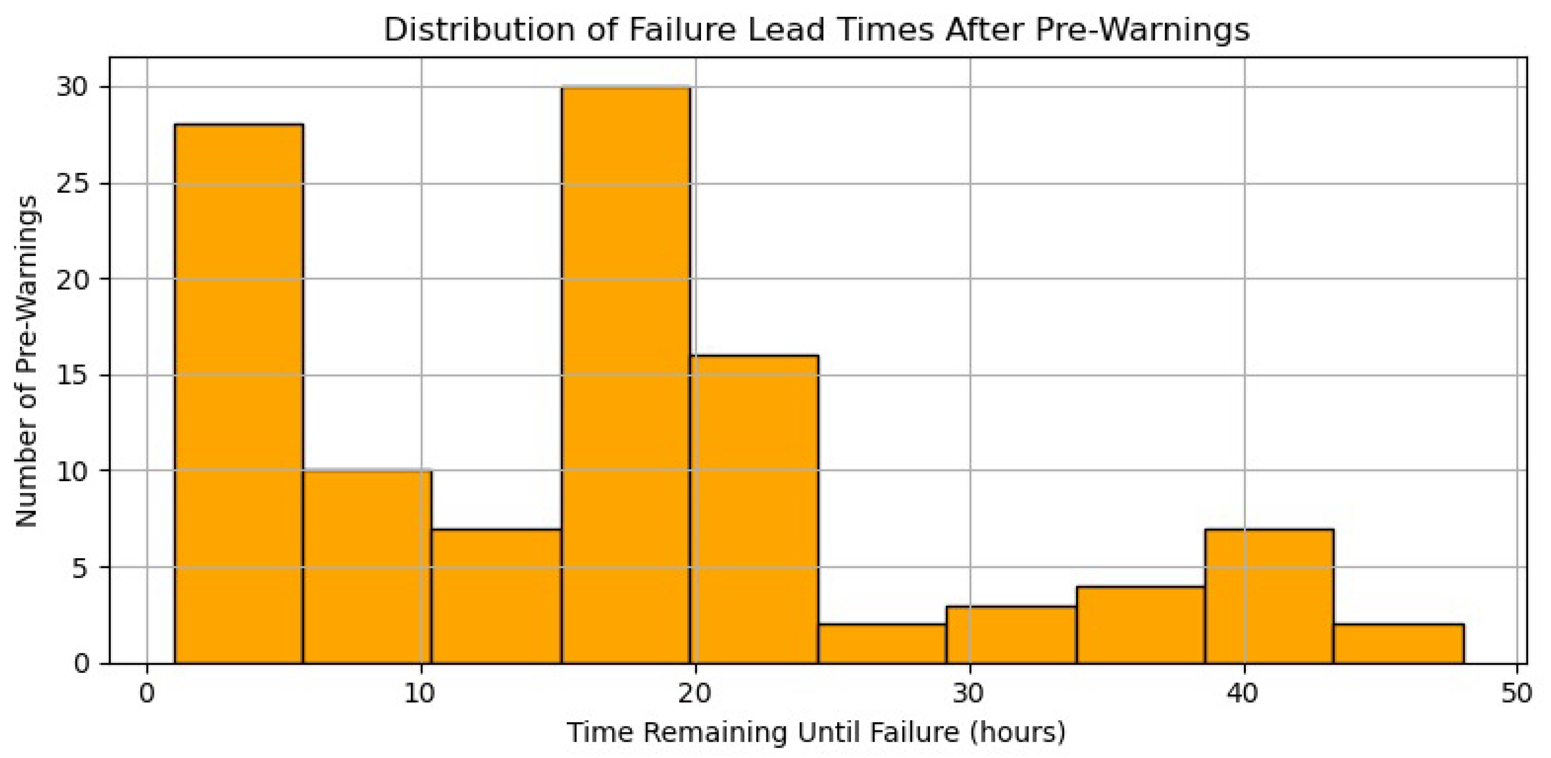
When examining the distribution of time remaining until failure in Figure 15, taking into account the differences between the time of failure and the warning times, most failures occur within 1–5 h after the warning. This output indicates that there are situations requiring immediate intervention. Subsequently, a 15–20 h advanced warning occurred. The system issued a warning, but the failure occurred the next day, not immediately. The occurrence of an anomaly after a certain period of time indicates the accumulation of hidden damage. This situation has been evaluated as output that can be included in the daily periodic maintenance list. Finally, it is observed that failures occur between 30 and 48 h after the warning. This situation offers ideal intervention opportunities. Predictive maintenance can be performed with the model to be trained as a result of the early warnings that occur.
Figure 15.
Failure time distribution after early warning.
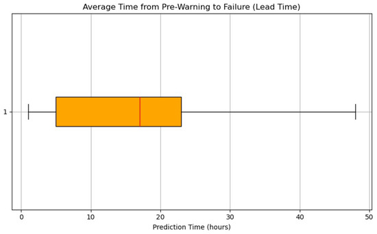
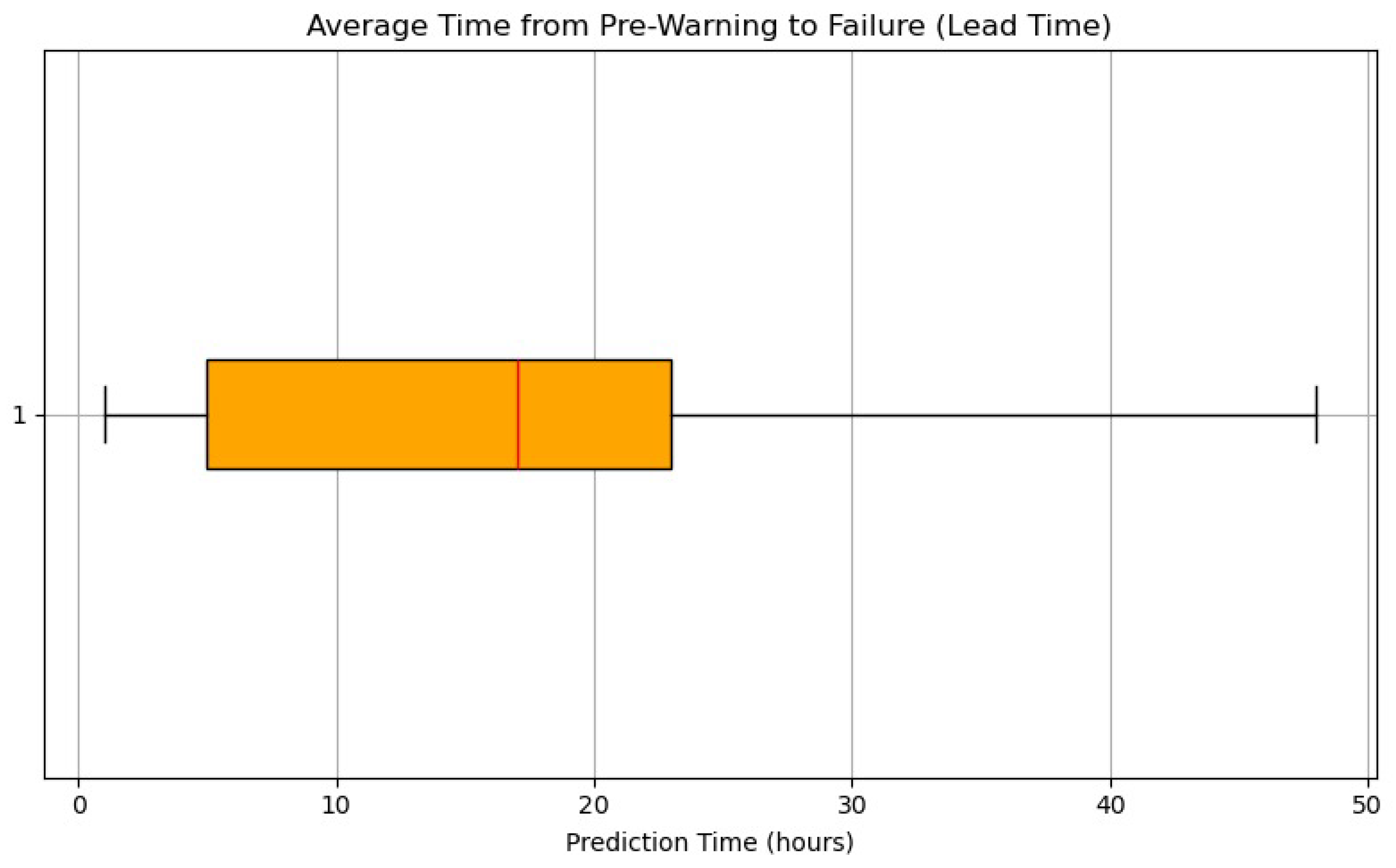
When the box plot of the average time from pre-alert to failure is statistically analyzed, it is seen that the median (red line) is 17 h, the 50% range is 5–25 h, and the outlier is 48 h (see Figure 16). The fact that the system can operate for such a long period demonstrates the success of the matching performed. This means that when the system issues a warning, the operator can be notified 17 h in advance.
Figure 16.
Statistical box plot of the time remaining from the pre-warning to the failure.
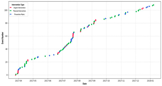
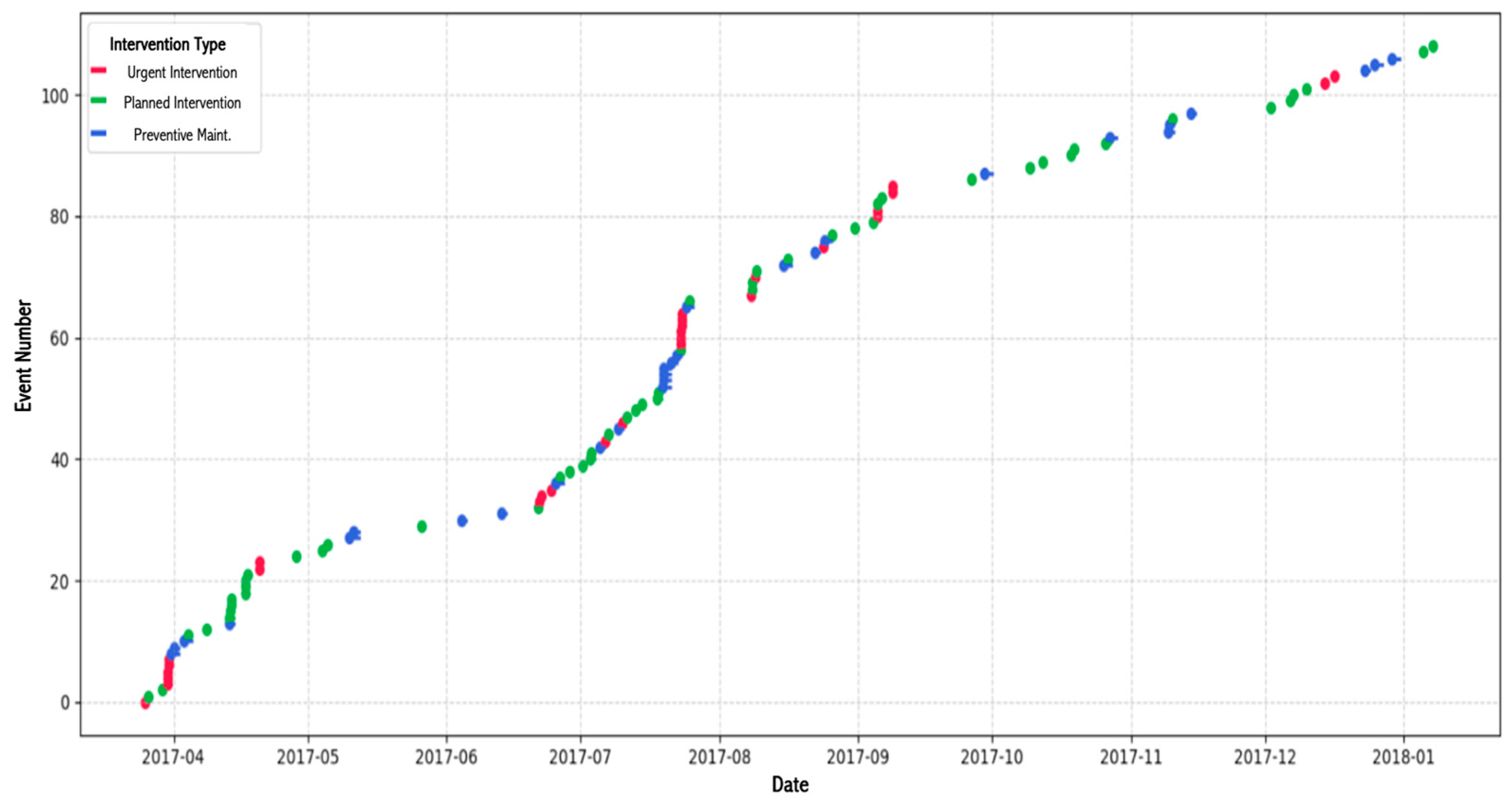
Early warnings are classified into intervention categories as follows: if they occur 5 h or more in advance, they require emergency intervention; if they occur 25 h or more in advance, they require planned intervention; and if warnings are received between 25 and 48 h in advance, they require preventive maintenance.
The existence of different intervention opportunities in each period indicates dynamic risk, as shown in Figure 17. Furthermore, the fact that most emergency interventions occur during the summer months may be a seasonal constraint. The most common scenario is that intervention will occur without significant delay, offering the most efficient operational intervention window.
Figure 17.
Time-dependent distribution of intervention types.
3.5. Model Selection and Training
Testing and selecting the models required to convert the warning system, whose foundations were laid through feature engineering, into an algorithm-based classification and prediction system, and training the models decided to be used, is the starting point for the final foundation of a predictive system.
Model performance was evaluated using Accuracy, Precision, Sensitivity (Recall), and the F1-Score. Given the inherent class imbalance in anomaly detection (where normal data significantly outweighs failure data), the F1-Score was prioritized to ensure an optimal balance between minimizing false alarms (Precision) and ensuring all faults were detected (Sensitivity).
3.6. Classic Machine Learning Models and Performance Results
To validate the classification of these warnings, nine classical machine learning models were tested. The goal was to maximize the F1-Score, which balances Precision (avoiding false alarms) and Sensitivity (detecting all faults).
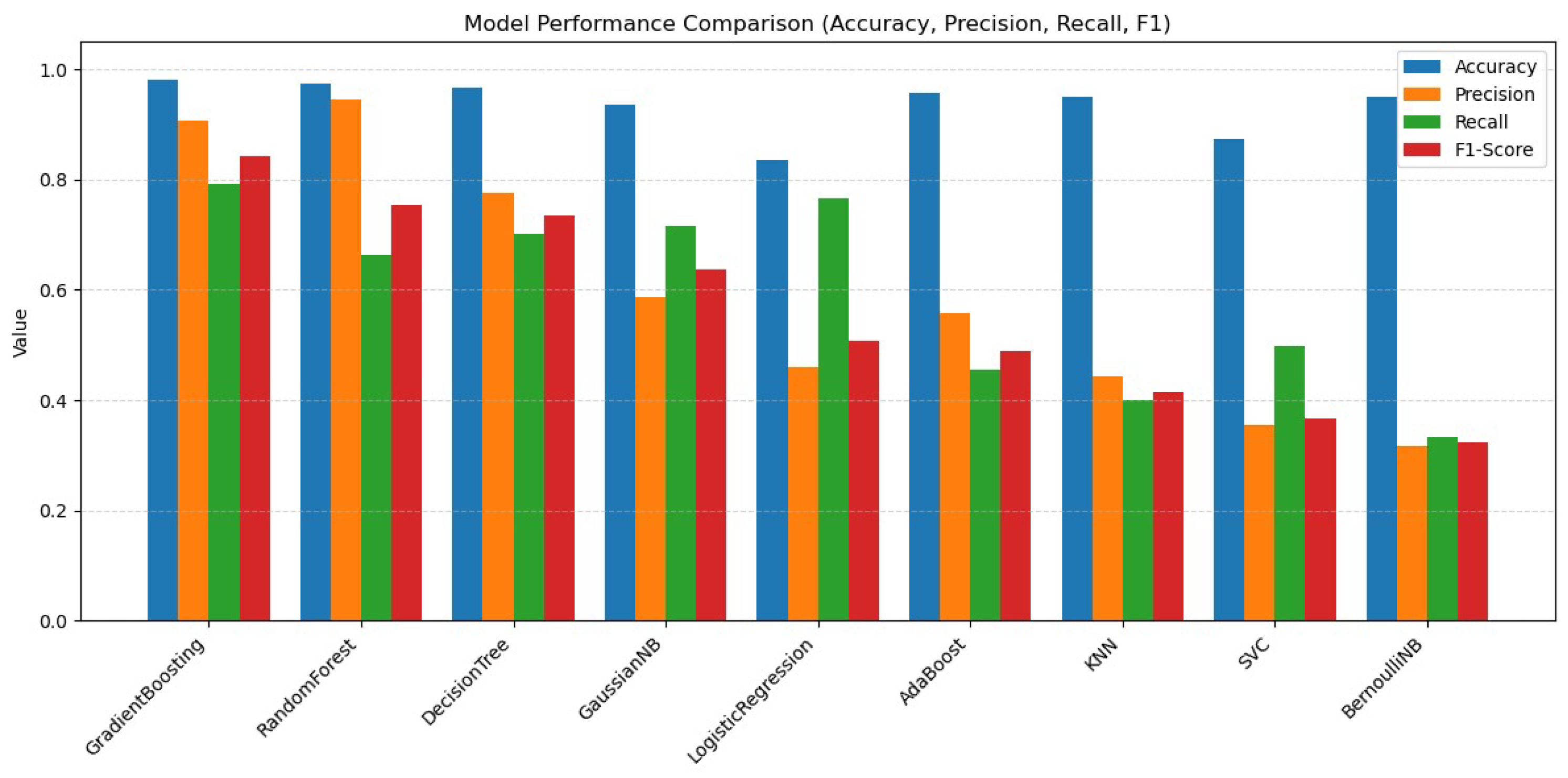
As detailed in Table 3, the Gradient Boosting Classifier achieved the highest performance with an F1-Score of 84.21%, followed by the Random Forest Classifier (77.61%). These ensemble methods proved superior to simpler linear models (Logistic Regression) and distance-based models (KNN) in handling the complex, non-linear relationships of the mill data.
Table 3.
Success rates of classical models.
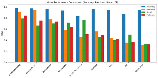
The results obtained by testing nine different machine learning algorithms show that the Gradient Boosting Classifier and Random Forest Classifier models can perform robust fault classification for the predictive maintenance system and provide real-time decision support thanks to their F1-Scores. Additionally, a graph comparing the performance of these models is shown in Figure 18.
Figure 18.
Performance comparison of machine learning models.
3.7. Deep Learning (LSTM) Implementation
Classic machine learning models operate based on data from a specific time, functioning in the present moment. Deep learning models such as Long Short-Term Memory (LSTM), on the other hand, are algorithms that can take time dependency into account. They can predict the probability of failure occurring in future hours based on the relationships between successive time steps.
To predict future failure states by analyzing temporal dependencies, Long Short-Term Memory (LSTM) networks were employed. Unlike standard RNNs, the LSTM architecture effectively manages long-term dependencies, making it ideal for time-series forecasting in a continuous production environment.
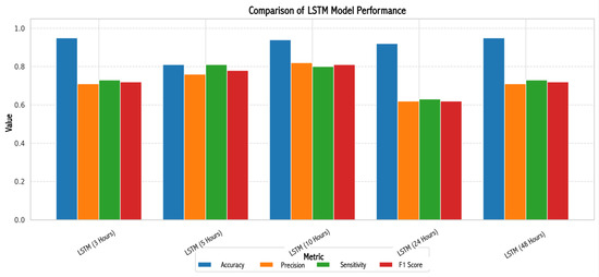
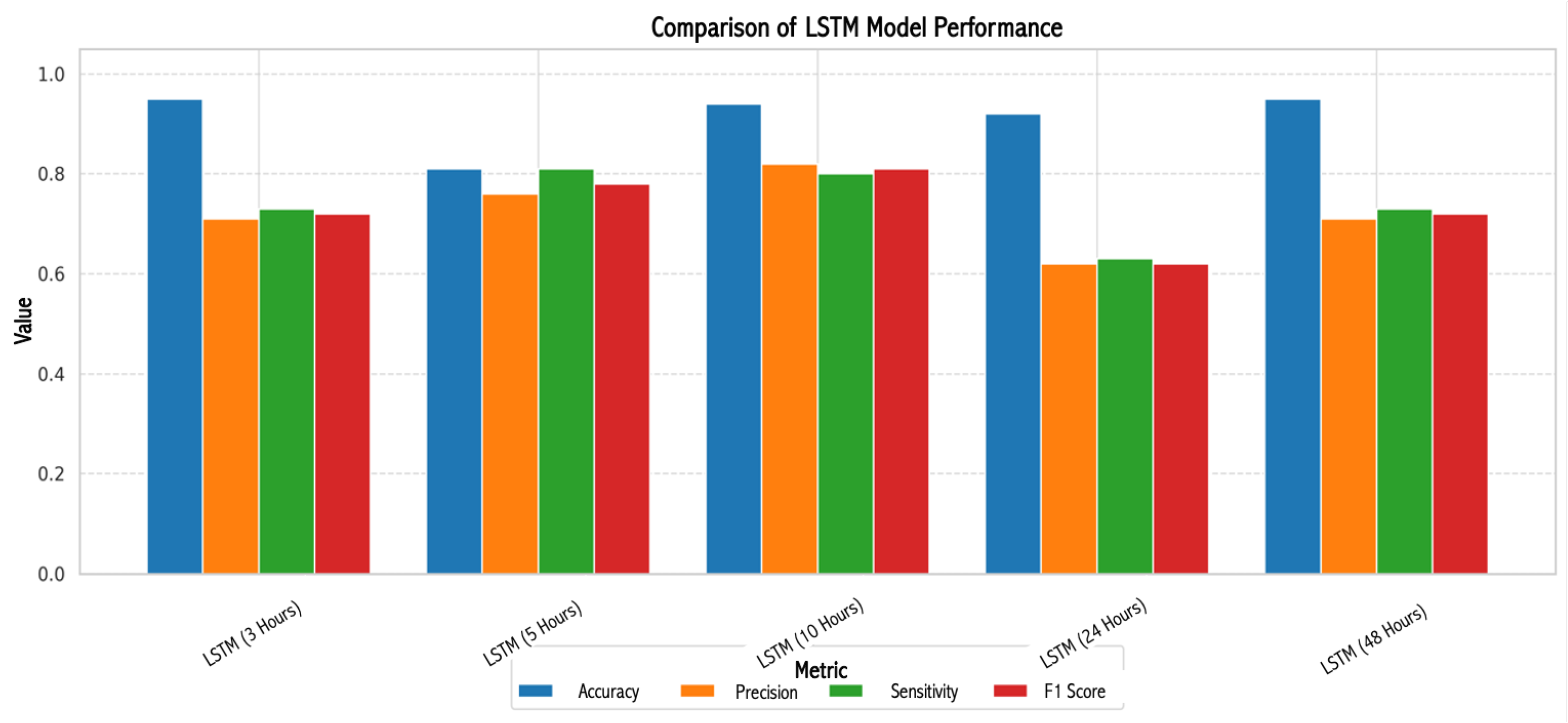
Five windows have been defined for analysis. Deep learning has been achieved using 3 h, 5 h, 10 h, 24 h, and 48 h windows. The 3 h windows focus on recent events and are effective in sudden failures and rapid changes. The 5 h window utilizes short history and transition times and is used in situations where warning systems are just starting. The 10 h window provides balanced analysis and maintains equilibrium between classes. The 24 h window is used for medium- to long-term trend tracking. The 48 h window was created for stable long-term predictions and serious disruptions. The success results of these windows are shown in Table 4. According to these results, the high accuracy rates of all models indicate that normal models are quite successful in terms of prediction. However, the main objective is for the models to detect abnormal situations. In this regard, the 10 h window showed the most balanced result with an 81% success rate.
Table 4.
Test results for Long Short-Term Memory (LSTM) models.
A comparison of the models in different windows is also shown in Figure 19. According to this, the most successful result is seen in the 10 h window. The 5 h window is also close to this situation. These two windows are considered strong models. This provides the possibility of using them in various applications.
Figure 19.
Success rates according to model windows.
3.8. Hybrid Model Architecture
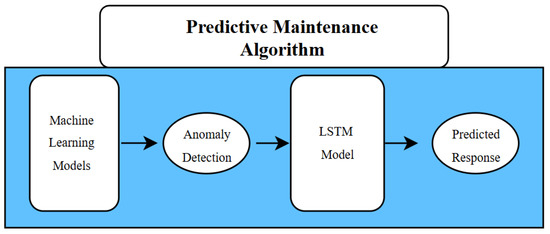
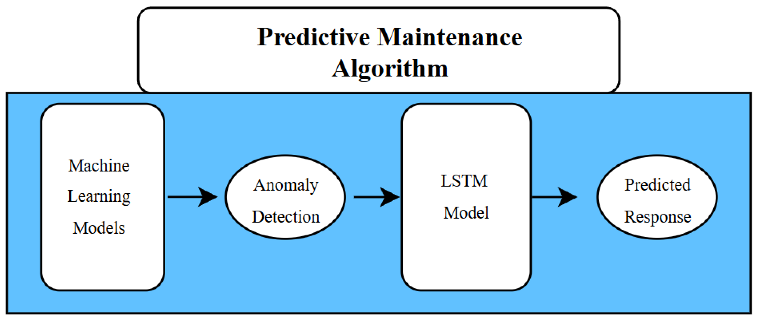
Classic machine learning algorithms that derive instantaneous data about the present based on sensor data from a specific time are an effective method for making decisions about the current situation. Long Short-Term Memory algorithms, on the other hand, are successful in predicting the future using real-time data. By using the variables resulting from anomaly classifications made with machine learning models as input information for the Long Short-Term Memory (LSTM) model, the forecasting process was more successful thanks to the powerful anomaly detection presented. Thanks to this combination, not only can maintenance failure times be predicted but also the type and location of maintenance, using informative features obtained from machine learning results in addition to raw data. Machine learning models perform real-time anomaly classification and feature selection, transferring their outputs to the deep learning system to enable forward-looking prediction. Figure 20 shows the flow chart of the hybrid model architecture.
Figure 20.
Flow chart of model.
3.9. Anomaly-Caused Downtime
When anomaly-caused downtime and the hours lost due to this downtime are examined in conjunction with the associated models in Table 5, which is the model output, it is seen that a total of 249 h of downtime was detected, with an average of 1.09 h and a maximum of 4.00 h. These downtimes can be predicted up to 3 to 48 h in advance using the five windows created. On average, a 17 h forecast is provided.
Table 5.
Downtimes predicted by the combined method.
The classification and prediction performed categorized the planning outputs as urgent, planned, and preventive. Some of the outputs of this predictive maintenance intervention action are shown in Table 6. Based on the 10 h window algorithm of this planning forecast, an F1-Score of 81% was obtained, revealing that 219.5 h of the 271 h downtime were definitely accurate.
Table 6.
Some of the reactions generated by the developed model.
Thanks to the combined model developed, downtime of 219.5 h can be prevented for a year’s worth of data.
3.10. Digital Twin Architecture
A digital twin is the synchronized modeling and testing of a physical system in a digital environment. Recent reviews in energy sectors [16] similarly highlight that the primary value of digital twin technology lies in reliability enhancement and operational feedback loops rather than static geometric representation. In the context of this study, the architecture represents an ‘Operational Digital Twin’, focusing on the replication of the system’s functional behavior and reliability state rather than its geometric physical attributes. This system was implemented in a Streamlit-based interface along with the developed models. Here, sensor data served as the data layer. The developed algorithms were used as the model layer. The interfaces created served as the visualization and decision layer. While traditional product digital twins often emphasize 3D object visualization, the proposed framework prioritizes the visualization of operational logic, providing alarm systems, maintenance recommendations, outputs, and live graphs for user interaction. All these components form the functional digital twin.
3.11. Layers of the Digital Twin Architecture
An architecture was developed that includes the sensors that collect data, the transmission of this data, the processing of the transmitted data, and the generation of results from this. The components of this architecture are based on four fundamentals and must work in an integrated manner for the entire system to function actively.
3.11.1. Physical Layer
The first layer collecting data from the mill consists of sensors. These devices monitor the status of equipment in the physical system and collect values.
3.11.2. Communication Layer
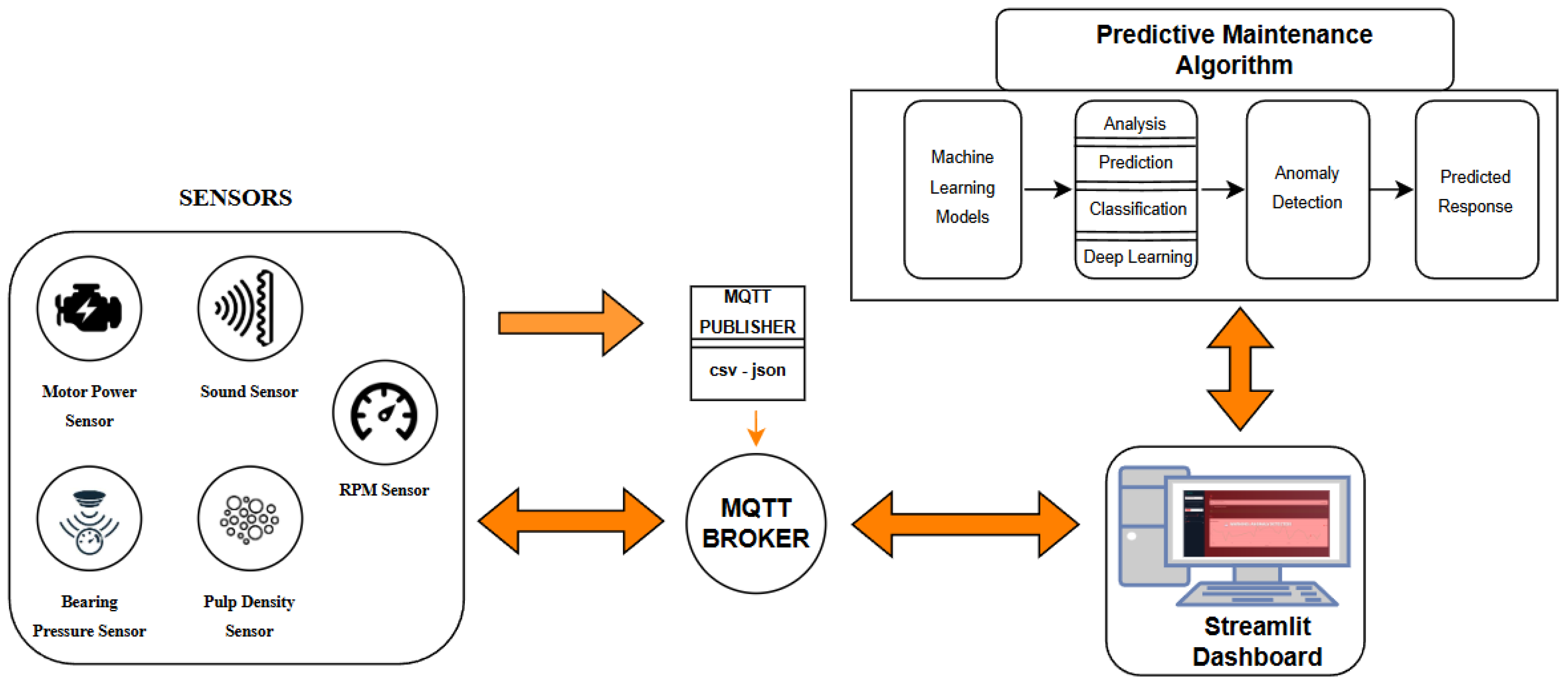
The communication layer is formed by the MQTT publisher converting data from sensors into CSV or JSON formats and transferring it to the MQTT broker. If the physical layer produces data in the format required by the MQTT broker, the data is sent directly here. Otherwise, the MQTT publisher first converts this data into the required format and then transfers it to the MQTT broker.
3.11.3. Analytical Layer
Data received from the MQTT broker is processed by the predictive maintenance algorithms created. As a result of processing, anomalies are detected, and forecasting operations are performed.
3.11.4. Decision Layer
All data and model outputs are presented to the necessary units through the interface created. The Streamlit panel serves as the interactive decision layer. It visualizes the ‘health state’ of the equipment through real-time time-series graphs, anomaly probability heatmaps, and intervention alerts, rather than static 3D spatial models. This allows operators to visualize the condition of the machine instantaneously.
3.12. Architectural Structure
The developed digital twin infrastructure transfers sensor data from the physical system to the MQTT broker, a central intermediary, via the MQTT-based lightweight messaging protocol. This data flow is transferred to the models developed via the Streamlit panel. The response of the predictive maintenance algorithms is sent to the Streamlit panel. The entire system is alerted via this panel, and the necessary responses are sent to the maintenance units and responsible authorities. The created architectural structure is shown in Figure 21.
Figure 21.
Architectural structure of the predictive maintenance system.
4. Discussion and Conclusions
This study presents three primary innovative outcomes contributing to the field of industrial reliability. 1. Methodological Innovation: The application of the MICMAC Systems Thinking approach to define sensor interdependencies prior to modeling. This shifted feature selection from a purely statistical exercise to a causality-driven process, ensuring that the model inputs represented actual physical constraints. 2. Algorithmic Hybridization: The development of a sequential hybrid architecture where Gradient Boosting Classifiers act as a ‘filter’ for anomaly detection, feeding refined state-data into LSTM networks. This approach solved the issue of class imbalance that typically degrades the performance of standalone deep learning models in failure prediction. 3. Operational Digital Twin Concept: The definition and implementation of a digital twin focused strictly on ‘Reliability State Synchronization’ rather than geometric visualization. This effectively bridges the gap between theoretical data science models and practical, floor-level maintenance decision-making.
Studies found in the literature were reviewed, and a large data set was used to address the shortcomings. The low cost of the established system was prioritized, and importance was placed on its uninterrupted operation. During the project development stages, the vast majority of factors that could affect the digital twin layers have been identified in detail using a Systems Thinking and analysis approach. Based on this approach, critical parameters such as data quality, employee competence, and sensor placement, which could disrupt system flow, were used to determine key points for the model, and Gradient Boosting and LSTM-based algorithms were developed using 400,000 data points.
The model results showed that machine learning models are successful in detecting anomalies in real time, while LSTM, one of the renewed neural networks, is successful in making predictions for the future. Minimum data requirements were defined by applying the Nyquist–Shannon Theorem for sampling frequency and empirically selecting a 10 h historical window based on LSTM model performance (Table 4). Shorter sequences failed to capture the necessary temporal dependencies to distinguish anomalies from noise.
As a result of the predictions made, a decision support structure was established with planned maintenance, emergency intervention, and preventive maintenance classifications. Thanks to forecasts averaging 17 h and extending up to 48 h, it was calculated that 219.5 h of downtime could be prevented over a one-year operating period, resulting in significant economic gains.
Author Contributions
Conceptualization, A.K. and M.M.K.; methodology, A.K. and M.M.K.; software, A.K.; validation, M.M.K.; formal analysis, A.K.; investigation, A.K.; resources, A.K.; data curation, M.M.K. and A.K.; writing—original draft preparation, A.K.; writing—review and editing, M.M.K.; visualization, A.K.; supervision, M.M.K.; project administration, M.M.K.; funding acquisition, M.M.K. All authors have read and agreed to the published version of the manuscript.
Funding
This research was funded by the Scientific Research Projects Department of Istanbul Technical University, grant number MGA-2024-45702.
Data Availability Statement
All data supporting the findings of this study are contained within the article (figures and tables).
Conflicts of Interest
The authors declare no conflicts of interest.
Abbreviations
The following abbreviations are used in this manuscript:
| AutoML | Automated Machine Learning |
| CSV | Comma-Separated Values |
| DL | Deep Learning |
| IoT | Information Technology |
| IT | Information Technology |
| JSON | JavaScript Object Notation |
| KNN | K-Nearest Neighbors |
| LSTM | Long Short-Term Memory |
| MICMAC | Matrix of Cross Impact Multiplications Applied to a Classification |
| ML | Machine Learning |
| MQTT | Message Queuing Telemetry Transport |
| PdM | Predictive Maintenance |
| RPM | Revolutions Per Minute |
| SAG | Semi-Autogenous Grinding |
References
- Dayo-Olupona, O.; Genc, B.; Celik, T.; Bada, S. Adoptable Approaches to Predictive Maintenance in Mining Industry: An Overview. Resour. Policy 2023, 86, 104291. [Google Scholar] [CrossRef] [Scilit]
- Veloso, B.; Ribeiro, R.P.; Gama, J.; Pereira, P.M. The MetroPT dataset for predictive maintenance. Sci. Data 2022, 9, 764. [Google Scholar] [CrossRef] [Scilit] [PubMed]
- Kruczek, P.; Gomolla, N.; Hebda-Sobkowicz, J.; Michalak, A.; Śliwiński, P.; Wodecki, J.; Zimroz, R. Predictive Maintenance of Mining Machines Using Advanced Data Analysis System Based on the Cloud Technology. In Proceedings of the 27th International Symposium on Mine Planning and Equipment Selection-MPES 2018; Springer: Berlin/Heidelberg, Germany, 2019; pp. 459–469. [Google Scholar]
- Elbazi, N.; Mabrouki, M.; Chebak, A.; Hammouch, F. Digital Twin Architecture for Mining Industry: Case Study of a Stacker Machine. In Proceedings of the IEEE Global Power, Energy, and Communication Conference (GPECOM 2022), Nevsehir, Turkey, 14–17 June 2022; pp. 232–237. [Google Scholar]
- Hadi, R.H.; Hady, H.N.; Hasan, A.M.; Al-Jodah, A.; Humaidi, A.J. Improved Fault Classification for Predictive Maintenance in Industrial IoT Based on AutoML: A Case Study of Ball-Bearing Faults. Processes 2023, 11, 1507. [Google Scholar] [CrossRef] [Scilit]
- Jacobs, J.A.; Mathews, M.J. Failure Prediction of Mine Compressors. J. Fail. Anal. Prev. 2019, 19, 976–985. [Google Scholar] [CrossRef] [Scilit]
- Sundaram, S.; Zeid, I. 3-Phased Predictive Maintenance Framework for Mining Operations. J. Ind. Appl. 2021, 34, 115–127. [Google Scholar]
- Hsu, J.Y.; Wang, Y.F.; Lin, K.C. Wind Turbine Fault Diagnosis and Predictive Maintenance through Statistical Process Control and Machine Learning. IEEE Access 2020, 8, 23427–23439. [Google Scholar] [CrossRef] [Scilit]
- Aqueveque, P.; Radrigan, L.; Morales, A.S.; Willenbrinck, E. Development of a Cyber-Physical System to Monitor Early Failures in Vibrating Screens. IEEE Access 2021, 9, 145866–145885. [Google Scholar] [CrossRef] [Scilit]
- Rihi, A.; Bainaa, S.; Mhadaa, F.; Elbachari, E.; Tagemouatic, H.; Guerboub, M.; Benzakour, I. Predictive Maintenance in Mining Industry: Grinding Mill Case Study. Procedia Comput. Sci. 2022, 207, 2483–2492. [Google Scholar] [CrossRef] [Scilit]
- Mutovina, N.; Nurtay, M.; Kalinin, A.; Tomilov, A.; Tomilova, N. Application of Artificial Intelligence and Machine Learning in Expert Systems for the Mining Industry: Literature Review of Modern Methods and Technologies. Int. J. Electr. Comput. Eng. (IJECE) 2025, 15, 3291–3308. [Google Scholar] [CrossRef] [Scilit]
- Guerroum, M.; Zegrari, M.; Masmoudi, M. Machine Learning for the Predictive Maintenance of a Jaw Crusher in the Mining Industry. In Proceedings of the IEEE International Conference on Technology Management, Operations and Decisions, Marrakech, Morocco, 24–26 November 2021; pp. 787–791. [Google Scholar]
- Nacchia, M.; Fruggiero, F.; Lambiase, A.; Bruton, K. A Systematic Mapping of the Advancing Use of Machine Learning Techniques for Predictive Maintenance in the Manufacturing Sector. Appl. Sci. 2021, 11, 2546. [Google Scholar] [CrossRef] [Scilit]
- Polverino, L.; Abbate, R.; Manco, P.; Perfetto, D.; Caputo, F.; Macchiaroli, R.; Caterino, M. Machine learning for prognostics and health management of industrial mechanical systems and equipment: A systematic literature review. Int. J. Eng. Bus. Manag. 2023, 15, 18479790231186848. [Google Scholar] [CrossRef] [Scilit]
- Mwale, W.; Liu, Z.; Chipusu, K. A Hybrid AI Framework for Integrated Predictive Maintenance and Mineral Quality Assessment in Mining. Appl. Sci. 2025, 15, 12222. [Google Scholar] [CrossRef] [Scilit]
- Chen, B.-Q.; Liu, K.; Yu, T.; Li, R. Enhancing Reliability in Floating Offshore Wind Turbines Through Digital Twin Technology: A Comprehensive Review. Energies 2024, 17, 1964. [Google Scholar] [CrossRef] [Scilit]

Disclaimer/Publisher’s Note: The statements, opinions and data contained in all publications are solely those of the individual author(s) and contributor(s) and not of MDPI and/or the editor(s). MDPI and/or the editor(s) disclaim responsibility for any injury to people or property resulting from any ideas, methods, instructions or products referred to in the content. |
© 2026 by the authors. Licensee MDPI, Basel, Switzerland. This article is an open access article distributed under the terms and conditions of the Creative Commons Attribution (CC BY) license.