Evaluation and Optimization of Manufacturing Supply Chain Resilience

Abstract

Digital transformation can improve supply chain sensing, but recovery depends on whether reliable information is converted into coordinated operational action. This study develops a simulation-based case study that integrates data-quality-adjusted indicator fusion, a six-dimensional resilience index, system dynamics, and phase-based constrained policy search. The case represents a component-intensive discrete-manufacturing network with 28 tier-1 suppliers, nine qualified alternatives, seven logistics nodes, and five product families. A reproducible 36-month supplier-product panel (5040 unit-month records) is generated from a fixed seed and an explicit machine-readable configuration; it is not presented as confidential company data. Completeness, timeliness, cross-source consistency, and out-of-sample predictive contribution are defined explicitly, and an event-preserving gate prevents reliability shrinkage from attenuating logged disruption signals. Twelve indicators measure robustness, redundancy, agility, visibility, collaboration, and adaptive recovery; time-to-recovery is reserved as an outcome rather than included in the input index. The dynamic model is solved at a 0.25-month step over a 24-month policy horizon. Under a compound supplier-capacity, demand, and logistics shock, the balanced phase-based portfolio increases minimum resilience from 0.490 to 0.680 and reduces time-to-recovery from 8.4 to 3.5 months relative to the efficiency baseline. At an equal 6.9% incremental-cost budget, the integrated portfolio retains a 0.029–0.071 advantage in minimum resilience over single-mechanism alternatives. Holdout replay, alternative weighting schemes, event-gate tests, parameter perturbations, and unseen shock combinations establish numerical robustness but do not constitute external empirical validation. The findings indicate, for this specified model and case, that visibility creates resilience value when coupled with response authority, supplier coordination, flexible capacity, and targeted buffers.

1. Introduction

Manufacturing supply chains are exposed to overlapping supplier failures, demand volatility, transport constraints, cyber dependence, and geopolitical risk. Resilience therefore cannot be reduced to average cost or on-time delivery; it concerns the capacity to resist, absorb, recover, and adapt while preserving essential service. Contemporary scholarship distinguishes resilience as both a measurable performance trajectory and an organizational process that changes the structure of the supply chain after disruption [1,2]. This distinction is particularly important in discrete manufacturing because production continuity depends on synchronized material availability, qualified alternatives, equipment capacity, logistics, and cross-tier information.

Recent evidence illustrates the scale of the operational problem. The European Investment Bank’s 2023 Supply Chain Survey covered approximately 1100 EU importers: 37% identified access to commodities and raw materials as a major obstacle, 34% reported logistics and transport disruption, and the logistics-disruption share reached 44% among firms importing from China [3]. These figures do not define the parameters of the present case, but they demonstrate why manufacturing firms combine digital tracking, inventory changes, and supplier diversification rather than relying on a single response.

Digital transformation changes the speed and scope with which firms sense and coordinate disruption. Industry 4.0 technologies can reduce information delay and improve ripple-effect analytics [4,5], while recent empirical studies associate supply chain digitalization with resilience through information processing, recovery capability, and inventory efficiency [6,7,8]. Digital capability, however, is not equivalent to operational recoverability. A firm may detect a supplier failure in real time yet remain unable to qualify a substitute, reallocate production, or release emergency inventory. Digital dependence can also introduce poor data quality, incompatible systems, cyber exposure, and uneven partner maturity.

The literature leaves three connected problems. First, many assessments remain static and do not separate input capabilities from recovery outcomes. Second, heterogeneous records are often aggregated without an explicit reliability rule, although operational systems, supplier portals, and public-risk feeds differ in missingness, latency, and consistency. Third, optimization studies frequently compare fixed portfolios or optimize one operational lever, leaving unclear how digital governance, collaboration, flexibility, and buffers should change across disruption phases. These limitations make it difficult to distinguish a real methodological gain from an outcome produced by higher spending or by relationships already embedded in a model.

The aim of this study is to develop and transparently test a simulation architecture that connects data reliability, diagnostic resilience measurement, dynamic feedback, and phase-specific managerial action. This study asks the following: (1) how can heterogeneous indicators be fused without suppressing genuine disruption signals; (2) how can a diagnostic index initialize and inform a system dynamics model without being confused with its state variables or validation outcomes; and (3) whether an integrated policy remains preferable when budgets are equal and shocks differ from the calibration scenario. The sequence is indicator definition, reliability adjustment, objective weighting, dynamic-model specification, holdout replay, disruption simulation, constrained phase-based search, and robustness testing.

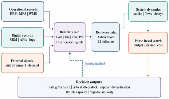
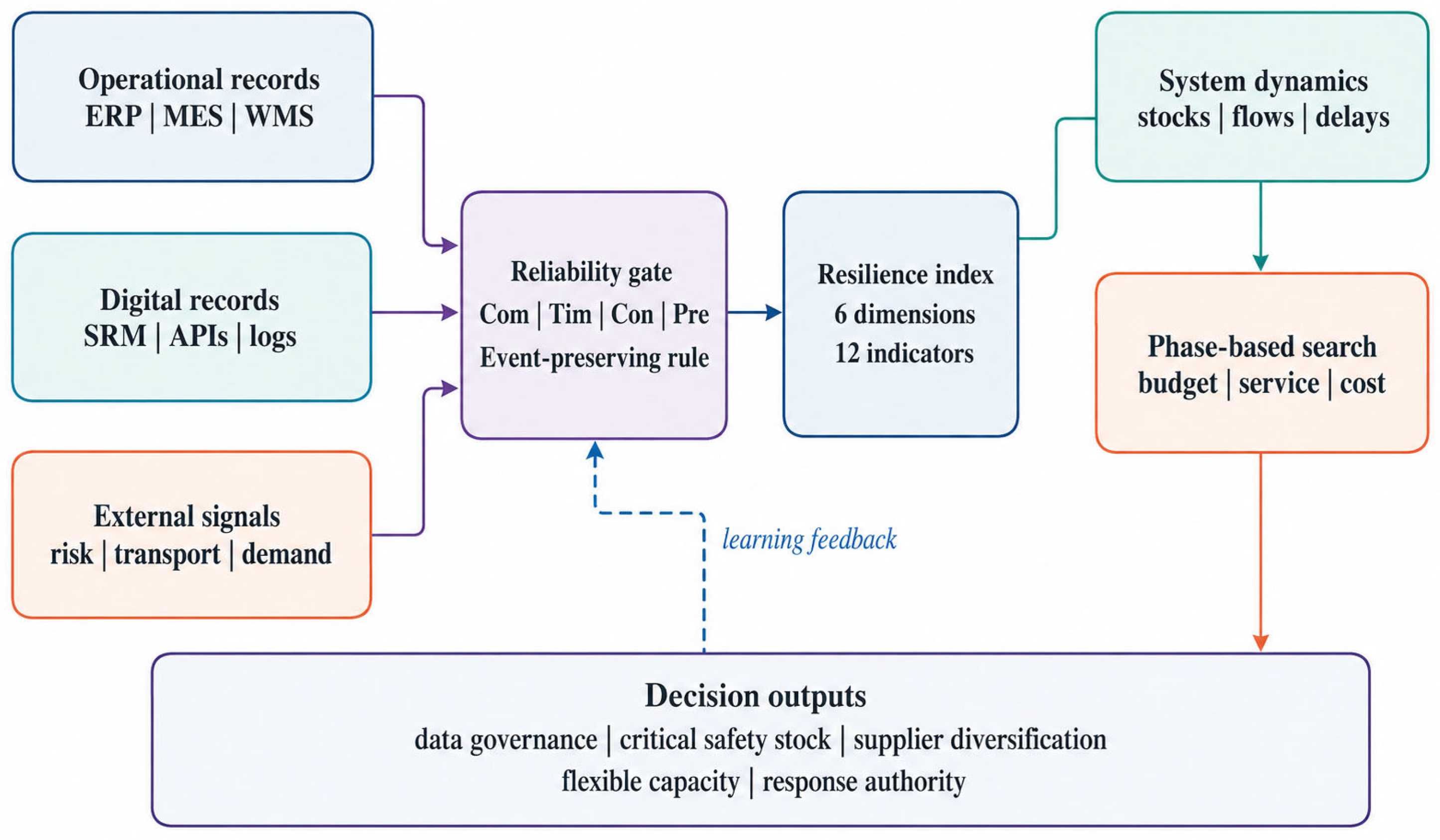
The contribution is methodological rather than a claim of universal empirical effect. The revised study (i) makes the case status and every data-generating assumption explicit; (ii) defines all reliability components and introduces an event-preserving gate; (iii) removes time-to-recovery from the input index to avoid double counting; (iv) reports indicator-level entropy, CRITIC, and combined weights; (v) supplies complete stock-flow, cost, service, parameter, and search specifications; and (vi) distinguishes calibration replay, scenario output, and managerial interpretation. Figure 1 maps the analytical stages to the decisions they can inform.

Figure 1. Integrated analytical workflow and mapping from data inputs to managerial decisions.

2. Literature Review and Research Positioning

2.1. Digital Transformation and Manufacturing Supply Chain Resilience

Digital supply chains combine connected records, analytical capability, traceability, and decision routines. Studies of digital supply chain capabilities and autonomous supply chains emphasize end-to-end visibility, interoperability, analytics, and staged autonomy [9,10]. Research on smart technologies likewise shows that technology creates value through organizational use rather than adoption alone [11]. Supply chain analytics can improve transparency [12], and traceability can support faster detection and accountability [13], but transparency is beneficial only when partners share compatible data and response procedures [14].

Recent evidence strengthens the contingency argument. Digitally driven capability is more effective when aligned with supply chain governance [15], and multiple technologies contribute through different resource and action pathways rather than as an undifferentiated digitalization score [7]. The present model therefore separates digital capability, data quality, visibility, supplier collaboration, production flexibility, and inventory buffering. Their positive links are model assumptions supported by prior theory; simulation results show the consequences of those assumptions and should not be interpreted as independent causal confirmation.

2.2. Dynamic and Simulation-Based Approaches

Simulation research captures disruption propagation, delayed recovery, and policy interactions that are difficult to observe in static indices. Agent-based work models financial ripple effects across adaptive networks [16], digital twins support supply chain stress testing [17], and recent system-dynamics optimization combines dynamic recovery models with reinforcement learning [18]. Broader reviews nevertheless identify recurring shortcomings: incomplete model equations, limited validation evidence, and sensitivity tests that do not cover parameter, initial-state, and policy-preference uncertainty [19,20].

System dynamics is appropriate when accumulation, feedback, and implementation delay are substantively important. It is less suitable for tracing detailed node-to-node contagion than a network or agent-based model. The present study uses an aggregate focal-network architecture and makes that boundary explicit. It adds a reliability-adjusted diagnostic layer and a transparent grid-search policy layer rather than claiming greater predictive accuracy than data-intensive machine-learning or network models.

2.3. Collaboration, Flexibility, Weighting, and the Research Gap

Collaboration can strengthen joint visibility, decision synchronization, and recovery [21], while visibility and flexibility act as complements under uncertainty [22]. Agility and responsiveness similarly support resilience, but their value depends on the disruption type and available resources [23]. These findings motivate a configurational model, yet they do not establish that every integrated portfolio is efficient. An equal-budget comparison is required to determine whether an integrated scenario performs well because of allocation or simply because it spends more.

Objective weighting also requires transparency. Entropy weights represent information dispersion, whereas the CRITIC method combines contrast intensity with inter-criterion conflict [24,25]. Averaging these weights is a modeling choice, not an automatic truth. The present study therefore reports both sets, uses equal mixing only as the primary symmetric specification, and repeats the evaluation under equal, entropy, CRITIC, and combined weights.

The methodological choices also draw on established and recent evidence. The stock-flow formulation follows the feedback and accumulation principles of system dynamics [26]. Disruption simulation has been used to estimate epidemic propagation [27], while Industry 4.0 and analytics research links digital capability to resilience, but cautions that technology effects depend on organizational use and evidence quality [28,29]. Manufacturing and procurement studies report positive digitalization associations [30,31], whereas early technology disappointment highlights integration and governance frictions [32]. These findings extend classic resilience and risk-management arguments [33,34], and systematic reviews show why explicit trajectories, assumptions, and quantitative validation remain necessary [35,36].

2.4. Recent Empirical and Digital-Twin Evidence and Synthesis of the Research Gap

Recent studies published after much of the foundational literature reinforce the need for a contingency view. Qi et al. [37] report a positive association between enterprise digital transformation and supply chain resilience, with heterogeneous effects across ownership and marketization contexts. Ge and Bao [38] show that digital transformation can propagate through vertical supply-chain relationships by improving supply–demand alignment and supplier innovation. However, the evidence is not uniformly positive: Jia and Li [39] find that digital collaboration can be negatively associated with resilience and that the relationship varies with government support and firm characteristics. Zhang et al. [40] identify supply chain collaboration as a mediator and social capital as a moderator of the digital transformation–resilience link, while Hossain et al. [41] find that digital-twin technologies and disruption-mitigation strategies both support resilience and that strategic fit significantly conditions the digital-twin–resilience relationship. Taken together, these studies indicate that digitalization is an enabling resource whose resilience value depends on governance, interorganizational coordination, and the ability to convert information into action rather than a direct technological effect.

Recent digital-twin research adds operational depth to this argument. Corsini et al. [42] integrate simulation, machine learning, and metaheuristic optimization to update replenishment parameters under disruption, demonstrating the value of adaptive decision support relative to static settings. Malekzadeh et al. [43] develop a supply-chain digital twin to analyze immediate and long-term disruptions in a multi-echelon manufacturing context and compare recovery strategies. These studies show how data-driven simulation can move from monitoring toward adaptive decision support. Their decision spaces, however, are organized around specific replenishment or recovery structures. They do not simultaneously connect observation-level data reliability, a multidimensional diagnostic resilience index, bounded stock-flow feedback, and phase-specific allocation across information, supplier, capacity, collaboration, and buffer levers.

Another gap concerns the quality of the information used to produce a resilience diagnosis. The transparency literature shows that analytics and traceability can improve visibility [12,14], and reviews of artificial intelligence and big-data analytics stress the value of richer information processing [29]. At the same time, technology-adoption research shows that integration problems, inconsistent data, governance frictions, and implementation conditions can limit expected benefits [32]. Most empirical studies nonetheless operate with firm-level constructs or already-assembled indicators; they rarely model, at the observation level, whether a disruption signal is complete, timely, cross-source consistent, and sufficiently reliable without suppressing genuine shocks. This distinction is important because increasing data volume is not equivalent to increasing decision quality. The reliability-adjusted fusion layer in the present study is intended to address this measurement-to-decision gap rather than to serve as another general digitalization index.

Taken together, the literature can be differentiated along four dimensions: evidence base, treatment of data quality, representation of dynamic mechanisms, and form of policy search. Survey and listed-firm studies provide external association evidence but usually do not reproduce disruption trajectories. Agent-based, network, and digital-twin models represent propagation or operational adjustment more explicitly, but often optimize a narrow set of controls. System dynamics captures feedback, accumulation, and delay, yet prior applications do not generally connect reliability-adjusted indicator fusion with phase-specific multi-lever governance and an equal-budget comparison. The present study therefore targets the intersection of these streams. Its claim is not algorithmic superiority or universal causality; it is a transparent architecture in which data-quality treatment, diagnostic measurement, dynamic simulation, and constrained phase-based decisions can be inspected separately.

Table 1 positions the contribution against closely related approaches. The distinctive element is not the use of system dynamics alone, but the explicit connection among data-quality treatment, diagnostic measurement, phase-based decisions, equal-budget comparison, and evidence-bounded interpretation.

Table 1. Comparison with closely related research streams.

Study	Evidence Base	Data-Quality Treatment	Dynamic Mechanism	Policy Search	Main Limitation Relative to This Study
Ivanov et al. [5]	Conceptual and analytical	Not an indicator-level gate	Ripple-effect analytics	No integrated phase search	Does not link data reliability to a composite diagnostic index
Zhao et al. [6]	Firm survey/empirical model	Measurement validation	Mediation model	No	Estimates associations but not disruption trajectories
Wu et al. [7]	Multi-technology empirical study	Construct-level validation	Resource–action–performance	No	Does not model delayed stock-flow recovery
Tian and Cui [8]	Quasi-natural network study	Administrative-data construction	Network mechanisms	No	Causal policy evidence but no operational policy optimization
Proselkov et al. [16]	Agent-based network model	Input calibration	Node and financial ripple effects	Scenario comparison	Rich topology; no reliability-adjusted indicator fusion
Bussieweke et al. [18]	System dynamics and reinforcement learning	Secondary-data calibration	Dynamic inventory/recovery	Adaptive RL	Focuses recovery orders rather than multi-lever data/operations governance
Qi et al. [37]	Listed-firm empirical panel	Constructed digitalization and resilience measures	Econometric heterogeneity analysis	No	External association evidence, but no disruption trajectory or operational policy schedule
Jia and Li [39]	Listed-firm empirical panel	Digital-collaboration construct	Moderation by government support and firm characteristics	No	Shows contingency and possible adverse association, but no operational dynamic mechanism
Hossain et al. [41]	Manufacturing survey and PLS-SEM	Construct-level survey validation	Dynamic-capability and strategic-fit relationships	No	Empirical fit evidence, but no disruption trajectory or phase-based allocation
Corsini et al. [42]	Digital twin, simulation, and machine learning	Operational-data/model inputs	Disruption and replenishment dynamics	Metaheuristic parameter optimization	Specific replenishment controls; no reliability-adjusted multidimensional diagnosis
Malekzadeh et al. [43]	Multi-echelon digital-twin case	Input calibration/model data	Immediate and long-term disruption simulation	Recovery-strategy comparison/optimization	Scenario-specific recovery focus; no reliability gate or phase-based multi-lever governance
Present study	Reproducible simulation case	Four-component reliability plus event gate	Bounded stock-flow model	Three-phase constrained grid search	Aggregate and simulation-based; no external empirical validation

3. Materials and Methods

3.1. Research Design and Separation of Analytical Roles

The study separates four object types. Inputs are generated operational indicators, policy settings, and exogenous shock functions. State variables are the bounded stocks in the system dynamics model. Diagnostic measures are the static resilience index and its six dimensions. Validation outcomes are replay error, minimum resilience, time-to-recovery (TTR), cumulative service loss, and cost. TTR is not used as an input indicator. This separation removes the double counting present when recovery time appears both inside the resilience index and in the optimization objective.

The research design has four stages. Reliability-adjusted fusion prepares the indicator matrix; diagnostic evaluation locates weak dimensions; system dynamics translates those dimensions into a causal trajectory; and phase-based search selects actions under budget and service constraints. Table 2 links each stage to a concrete decision rather than treating the framework as a generic sequence.

Table 2. Research stages, analytical outputs, and focal managerial decisions.

Stage	Input	Method	Output	Decision Supported	Primary Owner
Data reliability	ERP-like, MES-like, supplier, logistics, and risk records	Completeness, timeliness, consistency, predictive contribution, event gate	Reliability-adjusted panel	Repair data feeds or retain event observations	Data/IT governance
Diagnostic evaluation	Twelve normalized indicators	Entropy, CRITIC, and alternative weights	Six dimensions and composite index	Identify the dominant capability gap	Supply chain planning
Dynamic simulation	Initial stocks, shocks, delays, policy inputs	Bounded stock-flow equations	Resilience, pressure, service, and cost paths	Test safety stock, flexibility, and response protocols	Operations and procurement
Phase-based optimization	Candidate controls and constraints	Coarse grid plus local refinement	Feasible phase schedule and cost frontier	Allocate budget and decision authority by phase	Senior management

3.2. Case Status, Unit of Analysis, and Data Provenance

This is a simulation-based case study, not an anonymized empirical company study. The case represents a component-intensive discrete manufacturer and is not assigned a country, named firm, or claimed observation period. Network counts—one focal manufacturer, 28 tier-1 suppliers, nine qualified alternatives, seven logistics nodes, and five product families—are design settings used to create a sufficiently heterogeneous but tractable test environment.

The unit indexed by i is a supplier-product-family stratum; j indexes the 12 indicators and t indexes month. A balanced 28 × 5 × 36 panel produces 5040 unit-month records and 60,480 indicator values. Months 1–24 form the training and calibration period. Within this interval, months 19–24 are used only as rolling one-step-ahead internal validation points when estimating predictive contribution; each forecast for month m is fitted using months 1 through m-1. Scaling bounds and dynamic-model calibration use training information only. Months 25–36 form an untouched temporal holdout reference series for behavior replay. The separate policy simulation uses a 24-month horizon. No personally identifiable, confidential, or human-subject data are used, and no expert panel is claimed. Parameters that cannot be estimated from the generated reference panel are labelled case-design assumptions and are varied in sensitivity analysis.

Baseline panel generation is specified separately from the subsequent defect-injection procedure. The complete indicator-level generation specification is maintained in a machine-readable data-generation configuration available from the corresponding author upon reasonable request. For each of the 12 indicators, this configuration records the baseline distribution and its parameters or support, supplier-product-family heterogeneity settings, temporal-dependence settings, aggregation rule, and the event/shock transformation used to create disruption-consistent changes. The executable generator reads these values directly from the configuration, so no unstated defaults are introduced by the code. Together with the fixed random seed 9 July 2026 and the network dimensions stated above, these materials define the pre-defect panel; missingness, reporting delay, cross-source inconsistency, and outlier mechanisms are then applied at the rates reported in the next paragraph.

The generator introduces controlled data-quality defects so that the reliability method can be tested: 2903 missing cells (4.8%), 3810 delayed cell reports (6.3%), 1875 cross-source inconsistencies (3.1%), and 423 statistical outliers (0.7%). Event tags identify 272 of the outliers as disruption-consistent changes; these values are retained. The remaining 151 non-event outliers are winsorized at the indicator-specific 0.5th and 99.5th percentiles. Appendix A Table A1 reports the formula, unit, source analogue, frequency, aggregation level, number of observations, and missing share for every indicator.

To support independent checking and full reproducibility, the complete data-generation configuration, executable panel-generation and calibration scripts, machine-readable long-format panel, parameter and scenario configuration, preprocessing, weighting, fusion, simulation, policy-search and robustness outputs, and environment specification are available from the corresponding author upon reasonable request. Panel generation and uncertainty sampling use the fixed seed 9 July 2026. The data-generation configuration records the exact indicator-level distributional assumptions, initialization ranges, heterogeneity and temporal-dependence settings, perturbation parameters, aggregation rules, and event-transformation settings required to reconstruct the declared simulation case. These materials document the implementation of the generated simulation case and are not presented as external company observations (Table 3).

Table 3. Provenance classes used in the revised study.

Value Class	Examples	Status in Inference	Reproducibility Treatment
Generated panel	Fulfilment, inventory days, latency, response times	Input to diagnostic evaluation and holdout replay	Complete generator specification available from the corresponding author upon reasonable request; seed, record count, and defect rates stated in text
Case-design assumption	Network size, shock magnitudes, policy bounds	Defines the simulation experiment	Reported explicitly and varied in sensitivity tests
Calibrated parameter	Transition, decay, and recovery coefficients	Governs state trajectories	Point value, range, unit, and source class in Table A2; calibration target, loss, and search procedure in Section 3.7; full calibration script available from the corresponding author upon reasonable request
Optimization output	Phase-specific policy intensities	Result conditional on model and constraints	Search grid, objective weights, budget, service floor, and evaluated combinations reported
Validation outcome	RMSE, minimum resilience, TTR, service loss	Tests numerical and behavioral adequacy	Calculated on holdout or unseen scenarios; not described as external validation

3.3. Preprocessing and Event Preservation

Daily and weekly synthetic events are aggregated to supplier-product-family months. Proportions use eligible-event denominators; durations use medians to limit skew; inventory coverage uses end-of-month available stock divided by the next 30-day expected consumption. A gap of one or two consecutive months is filled by the trailing three-month median within the same stratum. A gap longer than two months is estimated with a local-level state-space smoother fitted only to the training period. The primary results are repeated on complete cases and on the uncorrected event-tagged panel.

Outliers are detected using the robust standardized score $M_{ijt}=0.6745\left(x_{ijt}-{\mathrm{m}\mathrm{e}\mathrm{d}\mathrm{i}\mathrm{a}\mathrm{n}}_j\right)/{\mathrm{M}\mathrm{A}\mathrm{D}}_j$. A value is examined when $\left|M_{ijt}\right|>3.5$. It is retained without shrinkage when an event log exists or when at least two related sources move in the same direction within one month. This rule is essential in resilience analysis because an abrupt change can be the signal of interest rather than an error.

For a benefit indicator and a cost indicator, respectively, normalization uses training-period bounds winsorized at the 0.5th and 99.5th percentiles:

$$z_{ijt}^{+}=\mathrm{c}\mathrm{l}\mathrm{i}\mathrm{p} \left({\displaystyle \frac{x_{ijt}-L_j}{U_j-L_j}},0,1\right), z_{ijt}^{-}=\mathrm{c}\mathrm{l}\mathrm{i}\mathrm{p} \left({\displaystyle \frac{U_j-x_{ijt}}{U_j-L_j}},0,1\right)$$

(1)

The same $L_j$ and $U_j$ are frozen for the holdout period, preventing information leakage.

3.4. Data-Quality-Adjusted Fusion

The reliability index contains completeness (Com), timeliness (Tim), cross-source consistency (Con), and predictive contribution (Pre). The components are defined as follows:

$${\mathrm{C}\mathrm{o}\mathrm{m}}_{jt}={\displaystyle \frac{n_{jt}^{\mathrm{v}\mathrm{a}\mathrm{l}\mathrm{i}\mathrm{d}}}{n_{jt}^{\mathrm{e}\mathrm{x}\mathrm{p}\mathrm{e}\mathrm{c}\mathrm{t}\mathrm{e}\mathrm{d}}}}, {\mathrm{T}\mathrm{i}\mathrm{m}}_{jt}=\mathrm{e}\mathrm{x}\mathrm{p}\left(-d_{jt}/{\tau }_j\right), {\mathrm{C}\mathrm{o}\mathrm{n}}_{jt}=1-{\mathrm{m}\mathrm{e}\mathrm{d}\mathrm{i}\mathrm{a}\mathrm{n}}_i \left(\left|z_{ijt}^{\left(a\right)}-z_{ijt}^{\left(b\right)}\right|\right)$$

(2)

where $d_{jt}$ is reporting delay and ${\tau }_j$ is seven days for internal systems and 30 days for external feeds. Consistency compares paired normalized measures when two source analogues exist; if only one source exists, it is estimated from reconciliation with the accounting identity or adjacent process measure specified in Appendix A Table A1.

Predictive contribution is deliberately based on a criterion outside the composite index. A training-only AR(1) model predicts next-month service loss ${\mathcal{l}}_{i,t+1}=1-{\text{order-fulfilment rate}}_{i,t+1}$. Each indicator is then added separately. To avoid temporal leakage, predictive contribution is estimated entirely within months 1–24 using rolling-origin one-step-ahead validation. For validation months 19–24, both the benchmark and indicator-augmented models are fitted only on the preceding months, and their one-step-ahead squared errors are aggregated. The contribution of indicator j is the nonnegative proportional reduction in this training-period validation error, rescaled across indicators; months 25–36 never enter this calculation:

$${\mathrm{P}\mathrm{r}\mathrm{e}}_j={\mathrm{s}\mathrm{c}\mathrm{a}\mathrm{l}\mathrm{e}}_{\left[0,1\right]} \left[\mathrm{m}\mathrm{a}\mathrm{x} \left(0,{\displaystyle \frac{{\mathrm{R}\mathrm{M}\mathrm{S}\mathrm{E}}_0-{\mathrm{R}\mathrm{M}\mathrm{S}\mathrm{E}}_j}{{\mathrm{R}\mathrm{M}\mathrm{S}\mathrm{E}}_0}}\right)\right]$$

(3)

This definition avoids using the same resilience index as both predictor and outcome and keeps the temporal holdout independent of reliability estimation. The resulting predictive-contribution values are frozen before any processing or replay of months 25–36. The four components are combined using coefficients fixed before scenario evaluation:

$$r_{jt}=0.30\hspace{0.17em}{\mathrm{C}\mathrm{o}\mathrm{m}}_{jt}+0.25\hspace{0.17em}{\mathrm{T}\mathrm{i}\mathrm{m}}_{jt}+0.25\hspace{0.17em}{\mathrm{C}\mathrm{o}\mathrm{n}}_{jt}+0.20\hspace{0.17em}{\mathrm{P}\mathrm{r}\mathrm{e}}_j$$

(4)

The coefficients give slightly greater importance to missingness because an absent operational record cannot be corrected by freshness or consistency. They are not estimated to maximize the reported resilience results. Equal coefficients, each coefficient shifted by ±0.10 with renormalization, and windows of two, three, and six months are included in sensitivity analysis.

Let $E_{ijt}=1$ when a disruption-consistent event is verified. The fused feature is

$$u_{ijt}=E_{ijt}{z}_{ijt}+\left(1-E_{ijt}\right)\left[r_{jt}{z}_{ijt}+\left(1-r_{jt}\right){\tilde{z}}_{ij,t-1}^{\left(3\right)}\right]$$

(5)

where ${\tilde{z}}_{ij,t-1}^{\left(3\right)}$ is the median of the preceding three available months and excludes the current observation. Thus, low-reliability routine values are partially stabilized, whereas verified disruption values enter unchanged. This gate directly addresses the risk that reliability shrinkage could erase genuine shock signals.

3.5. Resilience Indicators and Objective Weights

The index covers robustness, redundancy, agility, visibility, collaboration, and adaptive recovery. Two indicators per dimension are retained to keep the diagnostic layer parsimonious and auditable. The indicators do not exhaust the construct; they operationalize mechanisms that are observable in an event-based discrete-manufacturing record. Content coverage is checked against four resilience functions—resist, absorb, respond, and learn—and variance-inflation factors are below 3.2 in the generated training panel. Table 4 gives the exact operational definition, unit, horizon, and direction of every indicator.

Table 4. Operational definitions of the resilience indicators.

Dimension	Code	Operational Definition	Formula or Denominator	Unit/Horizon	Direction
Robustness	ROB1	Fulfilment stability	$1-\mathrm{C}\mathrm{V}$ of monthly order-fulfilment rate, clipped to [0, 1]	Ratio; trailing 3 months	Benefit
Robustness	ROB2	Production plan adherence	Jobs completed within the released plan window/eligible released jobs	%; month	Benefit
Redundancy	RED1	Critical-material coverage	Available critical stock/forecast daily use	Days; month end	Benefit
Redundancy	RED2	Qualified alternative coverage	Critical components with at least one approved alternative/critical components	%; quarter, carried monthly	Benefit
Agility	AGI1	Production rescheduling cycle time	Median hours from approved change request to executable schedule	Hours; month	Cost
Agility	AGI2	Supplier-switching lead time	Median days from switch authorization to first accepted delivery	Days; event/month	Cost
Visibility	VIS1	Cross-system data latency	Median minutes from source event to reconciled planning record	Minutes; month	Cost
Visibility	VIS2	Traceability coverage	Order lines linked to supplier, batch, and logistics milestone/eligible lines	%; month	Benefit
Collaboration	COL1	Joint-plan adherence	Completed supplier planning cycles/scheduled cycles	%; month	Benefit
Collaboration	COL2	Supplier emergency response time	Median hours from alert issue to acknowledged feasible response	Hours; event/month	Cost
Adaptive recovery	REC1	Corrective-action closure rate	Disruption actions closed within 30 days/actions due	%; rolling 3 months	Benefit
Adaptive recovery	REC2	Learning implementation rate	Approved lessons incorporated into a standard process within 60 days/approved lessons	%; rolling 6 months	Benefit

TTR is intentionally absent from Table 4. It is calculated only after a disruption as the continuous time required for the dynamic resilience state to return to 95% of its pre-shock level. This change separates adaptive capability inputs from a realized recovery outcome.

For entropy weighting, $p_{ijt}=u_{ijt}/\sum _i{u}_{ijt}$, $e_j=-{\left[\mathrm{l}\mathrm{n}\left(n\right)\right]}^{-1}\sum _i{p}_{ijt}\mathrm{l}\mathrm{n}\left(p_{ijt}+ϵ\right)$, and $w_j^E=\left(1-e_j\right)/\sum _k\left(1-e_k\right)$ [25]. CRITIC information is $c_j={\sigma }_j{\displaystyle {\sum }_{k=1}^m}\left(1-{\rho }_{jk}\right)$ and $w_j^C=c_j/\sum _k{c}_k$ [24]. The primary combined weight is a symmetric pool:

$$w_j\left(\alpha \right)=\alpha w_j^E+\left(1-\alpha \right)w_j^C, \alpha =0.50$$

(6)

The diagnostic index is

$$R_i^{\mathrm{d}\mathrm{i}\mathrm{a}\mathrm{g}}\left(t\right)={\displaystyle \sum _{j=1}^{12}}{w}_j{u}_{ijt}, \sum _j{w}_j=1$$

(7)

Table 5 reports all indicator-level weights. The full-precision values, rather than displayed rounded values, are used in calculation. The dimension totals are 0.1810, 0.1395, 0.1720, 0.2100, 0.1530, and 0.1445, respectively.

Table 5. Indicator-level entropy, CRITIC, and combined weights.

Code	Entropy Weight	CRITIC Weight	Combined Weight	Dimension Contribution
ROB1	0.0940	0.1000	0.0970	0.1810
ROB2	0.0820	0.0860	0.0840
RED1	0.0690	0.0660	0.0675	0.1395
RED2	0.0730	0.0710	0.0720
AGI1	0.0880	0.0940	0.0910	0.1720
AGI2	0.0790	0.0830	0.0810
VIS1	0.1080	0.1040	0.1060	0.2100
VIS2	0.1020	0.1060	0.1040
COL1	0.0760	0.0820	0.0790	0.1530
COL2	0.0720	0.0760	0.0740
REC1	0.0790	0.0770	0.0780	0.1445
REC2	0.0780	0.0550	0.0665
Total	1.0000	1.0000	1.0000	1.0000

3.6. Link Between Diagnostic Evaluation and the Dynamic Model

The diagnostic index and dynamic resilience state are related but not identical. At the simulation start, the network-level mean of $R_i^{\mathrm{d}\mathrm{i}\mathrm{a}\mathrm{g}}\left(t\right)$ initializes $R\left(0\right)$. Dimension scores initialize the corresponding stocks: visibility initializes $V\left(0\right)$; collaboration initializes $C\left(0\right)$; the mean of the two agility indicators initializes $F\left(0\right)$ after reversing cost direction; and redundancy initializes $B\left(0\right)$. Digital capability $D\left(0\right)$ is initialized from system integration, update frequency, and interface coverage. The diagnostic index is recomputed only when a new monthly panel becomes available; within the 0.25-month simulation step, $R\left(t\right)$ evolves from the stock-flow equations. This is a measurement-to-state mapping, not two parallel resilience measures.

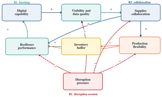
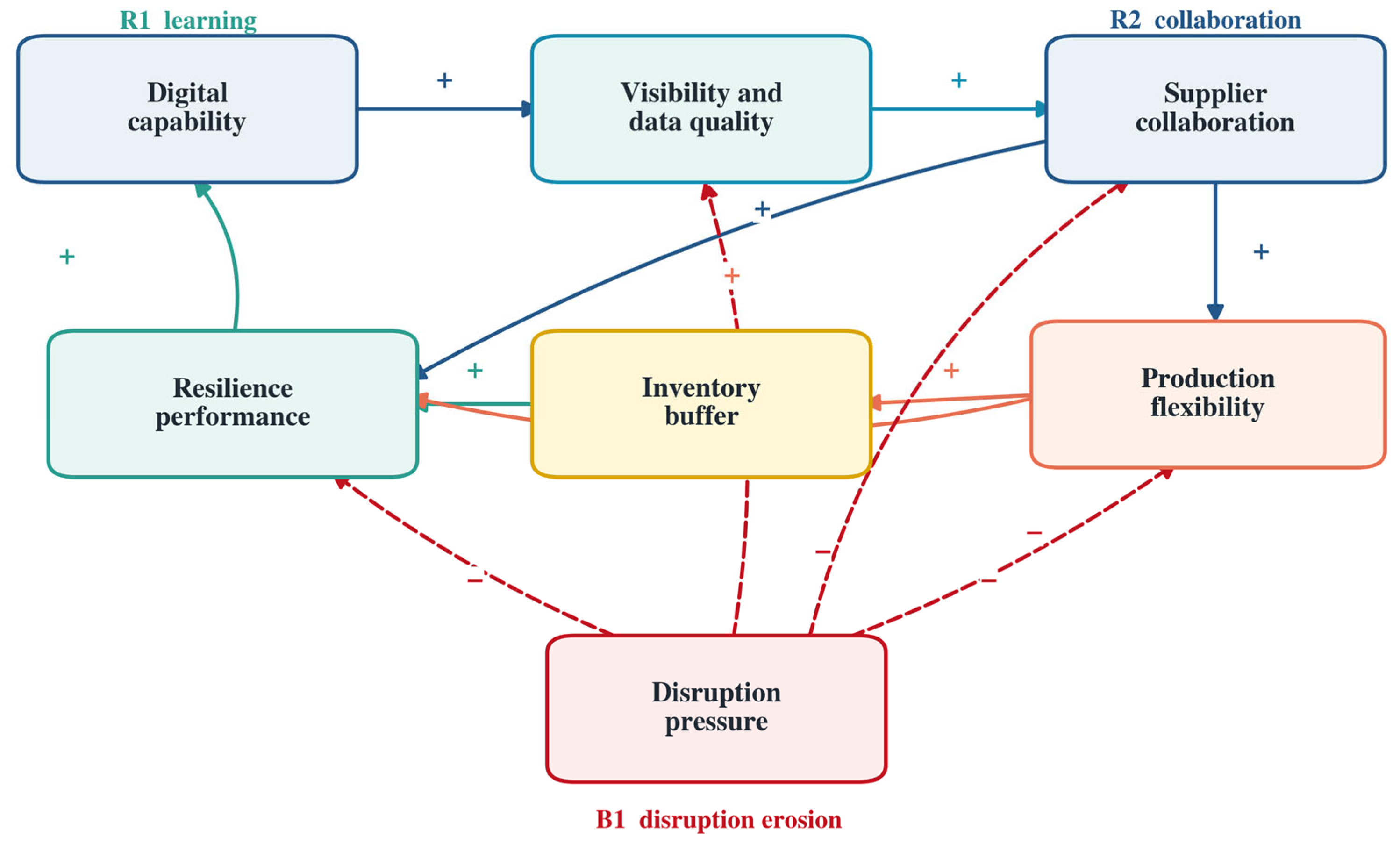
Figure 2 displays the causal structure. Positive signs indicate reinforcing effects and dashed red links indicate erosion by disruption pressure. The figure represents assumed causal directions grounded in prior research and managerial logic; it does not itself validate their empirical magnitude.

Figure 2. Causal feedback structure of the bounded system dynamics model.

3.7. Stock-Flow Equations and Parameterization

All stocks are bounded with $\mathrm{s}\mathrm{a}\mathrm{t}\left(x\right)=\mathrm{m}\mathrm{i}\mathrm{n}\left(1,\mathrm{m}\mathrm{a}\mathrm{x}\left(0,x\right)\right)$. Numerical integration uses fourth-order Runge–Kutta with $\Delta t=0.25$ month. The core stocks are digital capability $D$, visibility $V$, supplier collaboration $C$, production flexibility $F$, inventory buffer $B$, disruption pressure $P$, and dynamic resilience $R$. Data-quality governance $Q$, alternative-supplier intensity $A$, collaboration governance $G$, digital investment $I_D$, flexible-capacity investment $I_F$, and buffer target $B^{*}$ are controls or auxiliaries.

The capability stocks are

$$\dot{D}={\alpha }_D{I}_D\left(t\right)\left(1-D\right)-{\beta }_{D}D, \dot{V}={\alpha }_{V}DQ\left(t\right)\left(1-V\right)-{\beta }_{V}PV$$

(8)

$$\dot{C}={\alpha }_{C}VG\left(t\right)\left(1-C\right)-{\beta }_{C}PC, \dot{F}=\{{\alpha }_{F}D+{\gamma }_{F}C+{\eta }_F{I}_F\left(t\right)\}\left(1-F\right)-{\beta }_{F}PF$$

(9)

Inventory is governed by explicit replenishment, consumption, and obsolescence flows:

$$\dot{B}=\mathrm{R}\mathrm{e}\mathrm{p}-\mathrm{C}\mathrm{o}\mathrm{n}\mathrm{s}-\mathrm{O}\mathrm{b}\mathrm{s}$$

(10)

$$\mathrm{R}\mathrm{e}\mathrm{p}={\kappa }_B{\left[B^{*}\left(t\right)-B\right]}_{+}+{\xi }_{B}A\left(t\right)\left(1-B\right)$$

$$\mathrm{C}\mathrm{o}\mathrm{n}\mathrm{s}={\delta }_B\left[1+0.60s_d\left(t\right)+0.35P\right]B, \mathrm{O}\mathrm{b}\mathrm{s}=o_{B}B$$

(11)

where $s_d\left(t\right)$ is the normalized demand shock. Supplier-capacity loss $s_s\left(t\right)$, demand shock, and logistics delay $s_l\left(t\right)$ create disruption pressure, while visibility, collaboration, and alternatives dissipate it:

$$\dot{P}=s_s\left(t\right)+0.60s_d\left(t\right)+0.40s_l\left(t\right)-\left[{\mu }_0+{\mu }_{V}V+{\mu }_{C}C+{\mu }_{A}A\left(t\right)\right]P$$

(12)

The capability-supported resilience target and realized resilience dynamics are

$$R^{*}\left(t\right)=0.10D+0.18V+0.17C+0.18F+0.17B+0.20Q$$

(13)

$$\dot{R}={\rho }_R\left[R^{*}\left(t\right)-R\right]-{\psi }_{P}P\left[1-0.40B\right]-{\psi }_{K}K\left(t\right)$$

(14)

The quadratic incremental-cost rate $K\left(t\right)$ and service index are

$$K\left(t\right)=\sum _{k\in \{D,Q,A,F,B,G\}}{c}_k{\left[u_k\left(t\right)-u_k^0\right]}_{+}^2$$

(15)

$$\mathrm{S}\mathrm{e}\mathrm{r}\mathrm{v}\mathrm{i}\mathrm{c}\mathrm{e}\left(t\right)=\mathrm{s}\mathrm{a}\mathrm{t}\left[0.72+0.30R\left(t\right)+0.08B\left(t\right)-0.08P\left(t\right)\right]$$

(16)

Appendix A Table A2 reports every coefficient, unit, point value, permissible range, and source class. For parameters labelled “Calibration”, the generated training reference is the monthly network-level composite resilience trajectory obtained from the reliability-adjusted and objectively weighted indicator panel for months 1–24. Calibration minimizes the mean squared difference between that reference trajectory and the dynamic resilience state over the same 24 months; internal stock trajectories are not treated as additional calibration targets. Parameters labelled “Assumption” are held at their case-design point values during this fit. A deterministic bounded least-squares search is restricted to the ranges in Appendix A Table A2, and the lowest-loss feasible parameter vector is selected before values are rounded to two decimals for reporting. The exact search settings, stopping rules, and executable calibration script are available from the corresponding author upon reasonable request. Months 25–36 and all policy-scenario outputs are excluded from parameter calibration, and no scenario is excluded after calibration.

3.8. Phase-Based Constrained Optimization

The decision horizon is 24 months: normal operation (months 0–6), absorption (6–9), adaptation (9–14), and recovery (14–24). Normal settings are fixed; six controls can change at the start of each subsequent phase. The objective components are normalized to [0, 1], with TTR divided by 12 months and cost divided by the 7% budget ceiling:

$$\mathrm{m}\mathrm{a}\mathrm{x}J=0.30\hspace{0.17em}\overline{R}+0.30\hspace{0.17em}{R}_{\mathrm{m}\mathrm{i}\mathrm{n}}+0.20\left(1-{\displaystyle \frac{\mathrm{T}\mathrm{T}\mathrm{R}}{12}}\right)+0.20\left(1-{\displaystyle \frac{\mathrm{C}\mathrm{o}\mathrm{s}\mathrm{t}}{0.07}}\right)$$

(17)

$$\mathrm{s}.\mathrm{t}. 0\le u_k\left(t\right)\le 1, \mathrm{C}\mathrm{o}\mathrm{s}\mathrm{t}\le 0.07, \mathrm{S}\mathrm{e}\mathrm{r}\mathrm{v}\mathrm{i}\mathrm{c}\mathrm{e}\left(t\right)\ge 0.80, \left|u_{k,p}-u_{k,p-1}\right|\le 0.40$$

(18)

The 0.80 service floor is enforced after the exogenous impact step, so the model does not rule out the immediate physical effect of a shock. Cost is expressed as a fraction of baseline operating cost. The coefficients $\left(c_D,c_Q,c_A,c_F,c_B,c_G\right)=\left(16.5,11.0,20.0,18.3,14.6,11.0\right)$ convert squared normalized increments to percentage points of baseline operating cost and reproduce the 6.9% cost of the balanced schedule.

Search is deterministic. Each phase first evaluates five admissible values for each of six levers (15,625 combinations per phase). A local refinement evaluates the coarse optimum and ±0.05 for each lever (729 combinations per phase). Across three decision phases, 49,062 combinations are evaluated for the primary scenario. The search is repeated for continuity-priority, recovery-speed, and cost-priority objective weights. This staged search is computationally transparent but does not guarantee the global optimum of a fully continuous 18-dimensional control problem.

4. Experimental Design and Validation Protocol

4.1. Shock and Policy Scenarios

The calibration scenario starts in month 6 and lasts three months. It combines a 40% loss of one critical supplier’s capacity, a 25% demand increase in two product families, and a 20% delay on the primary logistics route. These magnitudes are case-design stress levels, not a claim that a comparable event occurred in an observed firm. Separate supplier-only, demand-only, logistics-only, short-severe, and long-moderate shocks are used as unseen evaluation scenarios.

Five policy logics are compared. S0 retains lean buffers and baseline digital settings. S1 emphasizes digital integration and data governance. S2 emphasizes alternatives, buffer, and flexible capacity. S3 emphasizes supplier coordination and shared response routines. S4 applies the integrated phase-based search. Table 6 separates the mechanisms and prevents the integrated case from being defined only as “more of everything.”

Table 6. Scenario definitions and primary mechanisms.

Scenario	Policy Logic	Levers Above Baseline	Levers Held Near Baseline	Intended Mechanism
S0	Efficiency baseline	None	All	Low cost; limited absorption and slow recovery
S1	Data integration	$I_D,Q$	$A,I_F,B^{*},G$	Faster sensing and more reliable information
S2	Redundancy-flexibility	$A,I_F,B^{*}$	$I_D,Q,G$	Physical absorption and reconfiguration
S3	Collaboration control tower	$Q,G$$; \mathrm{moderate} I_D$	$A,I_F,B^{*}$	Faster acknowledgement and synchronized action
S4	Integrated phase search	All, subject to constraints	None fixed	Allocate information and operational levers by phase

4.2. Calibration, Holdout Replay, and Extreme Conditions

Parameters are calibrated on months 1–24 of the generated reference panel and are frozen before any temporal-holdout calculation. Predictive contribution is also fixed beforehand from the rolling internal-validation procedure in Section 3.4. Months 25–36 are not used to adjust scaling bounds, model coefficients, reliability components or weights, objective weights, or policy values. This clarification makes the validation split explicit and does not change the reported numerical results, the S4 ranking, or the substantive conclusions. The balanced S4 schedule is then selected only under the declared compound calibration shock and frozen before the supplier-only, demand-only, logistics-only, short-severe, and long-moderate shock families are evaluated; no coefficient or control is refitted on those scenarios. This produces two design-separated checks: temporal holdout replay for numerical behavior and shock-family holdout evaluation for policy transfer. The reported RMSE, MAE, and R² remain internal statistics for a generated case and are not described as external empirical validation. Structural checks verify equation signs, units, bounds, and feedback direction, while Appendix A Table A3 reports numerical boundary tests.

Uncertainty analysis perturbs calibrated coefficients within the ranges in Appendix A Table A2, initial stocks by ±10%, implementation delays by ±50%, reliability coefficients, rolling windows, and all four weighting schemes. A Latin hypercube of 1000 parameter sets is used for interval results. Random seed 9 July 2026 is fixed for panel generation and uncertainty sampling. The executable configuration records the point value, range, source class, and constraint for each parameter so that the frozen evaluation protocol can be rerun without interpretive choices by the reader.

4.3. Outcomes and Role Separation

Average resilience and minimum resilience summarize the trajectory. TTR is the interpolated time from the shock onset until $R\left(t\right)$ first reaches 95% of the pre-shock mean and remains above it for two consecutive monthly observations. Cumulative service loss is $100\sum _{t\ge 6}{\left[R_0-R\left(t\right)\right]}_{+}/\left[R_0\left(T-6\right)\right]$. Incremental cost is the horizon-average of Equation (15). These are outcomes; none are an input to the diagnostic index.

The equal-budget test rescales S1–S3 within their own mechanism class until each uses the same 6.9% incremental budget as S4. This comparison isolates allocation logic from resource quantity. The unseen-scenario test applies the S4 schedule optimized on the calibration compound shock without re-estimating its parameters or policy values.

5. Results

5.1. Diagnostic Resilience and Weight Stability

Table 7 reports the dimension results using the full-precision combined weights. Visibility has the largest dimension weight (0.2100), followed by robustness (0.1810) and agility (0.1720). This ranking is generated by the contrast and correlation structure of the panel, not by a subjective priority assignment. The composite values are 0.7523 before the shock, 0.6120 during the shock, and 0.7723 during recovery. Reporting four decimals resolves the apparent discrepancy that arises when rounded dimension weights and scores are multiplied.

Table 7. Dimension weights and diagnostic resilience scores.

Dimension	Combined Weight	Pre-Shock	Shock Period	Recovery Period
Robustness	0.1810	0.820	0.610	0.780
Redundancy	0.1395	0.680	0.640	0.700
Agility	0.1720	0.750	0.580	0.740
Visibility	0.2100	0.790	0.660	0.830
Collaboration	0.1530	0.710	0.570	0.760
Adaptive recovery	0.1445	0.730	0.600	0.800
Composite (full precision)	1.0000	0.7523	0.6120	0.7723

Weight sensitivity is limited at the composite level (Table 8). The shock-period index ranges from 0.598 to 0.614 across equal, entropy, CRITIC, and combined weights; the dimension ranking changes only between robustness and agility. The S4 policy remains first under every scheme. The combined weighting result should therefore be read as one stable specification, not as uniquely correct.

Table 8. Weighting-scheme sensitivity.

Weighting Scheme	Pre-Shock R	Shock-Period R	Recovery R	S4 Minimum R	S4 Rank
Equal weights	0.751	0.614	0.774	0.674	1
Entropy	0.756	0.604	0.779	0.677	1
CRITIC	0.749	0.598	0.770	0.672	1
Combined (primary)	0.752	0.612	0.772	0.680	1

5.2. Behavioral Replay and Numerical Validation

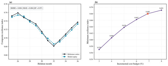
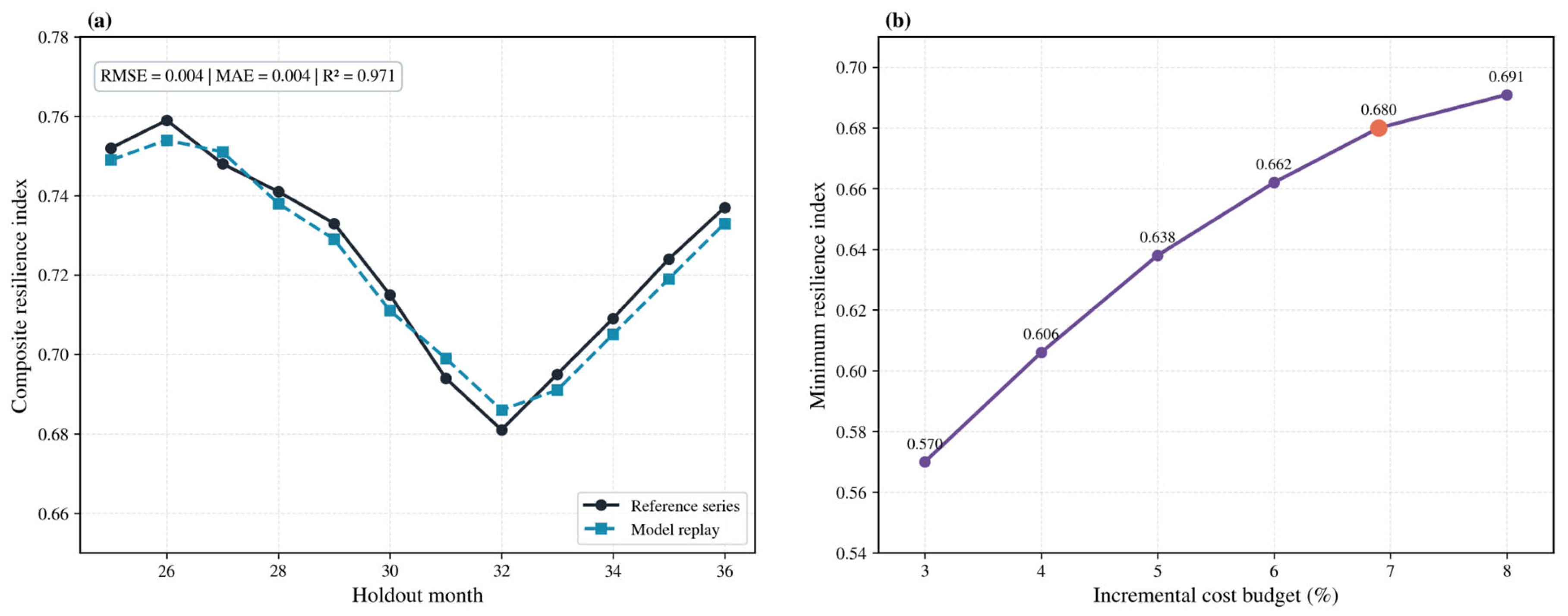
Figure 3a compares the 12-month holdout reference with model replay. RMSE is 0.004, MAE is 0.004, and R² is 0.971. Because months 25–36 are not used in predictive-contribution estimation, scaling, or parameter calibration, the replay is temporally separated from those model-preparation steps within the generated case. These statistics are used only as an implementation and parameter-behavior check; they are not evidence of external generalizability and are not used to select the policy schedule. The stronger protection against policy overfitting is the evaluation of the already-frozen schedule on the five unseen shock families in Section 5.5. Figure 3b shows diminishing returns along the cost–minimum-resilience frontier; increasing the cost budget from 6.9% to 8.0% adds only 0.011 to minimum resilience.

Figure 3. Internal validation and resource trade-off: (a) holdout reference versus model replay; (b) incremental-cost budget versus minimum resilience.

All state variables remain within [0, 1] under the extreme-condition tests. With no shock, $R\left(t\right)$ remains between 0.748 and 0.756. With a full supplier shock and zero response controls, minimum resilience falls to 0.311 without numerical instability. A zero budget reproduces S0; perfect data quality improves minimum resilience by 0.024 but cannot offset the absence of operational levers. These tests support structural plausibility rather than empirical truth.

5.3. Scenario Trajectories and Equal-Budget Comparison

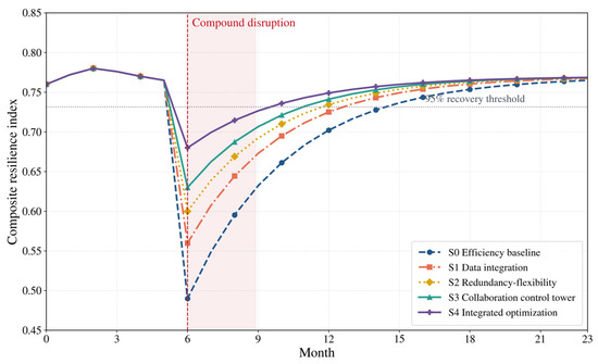
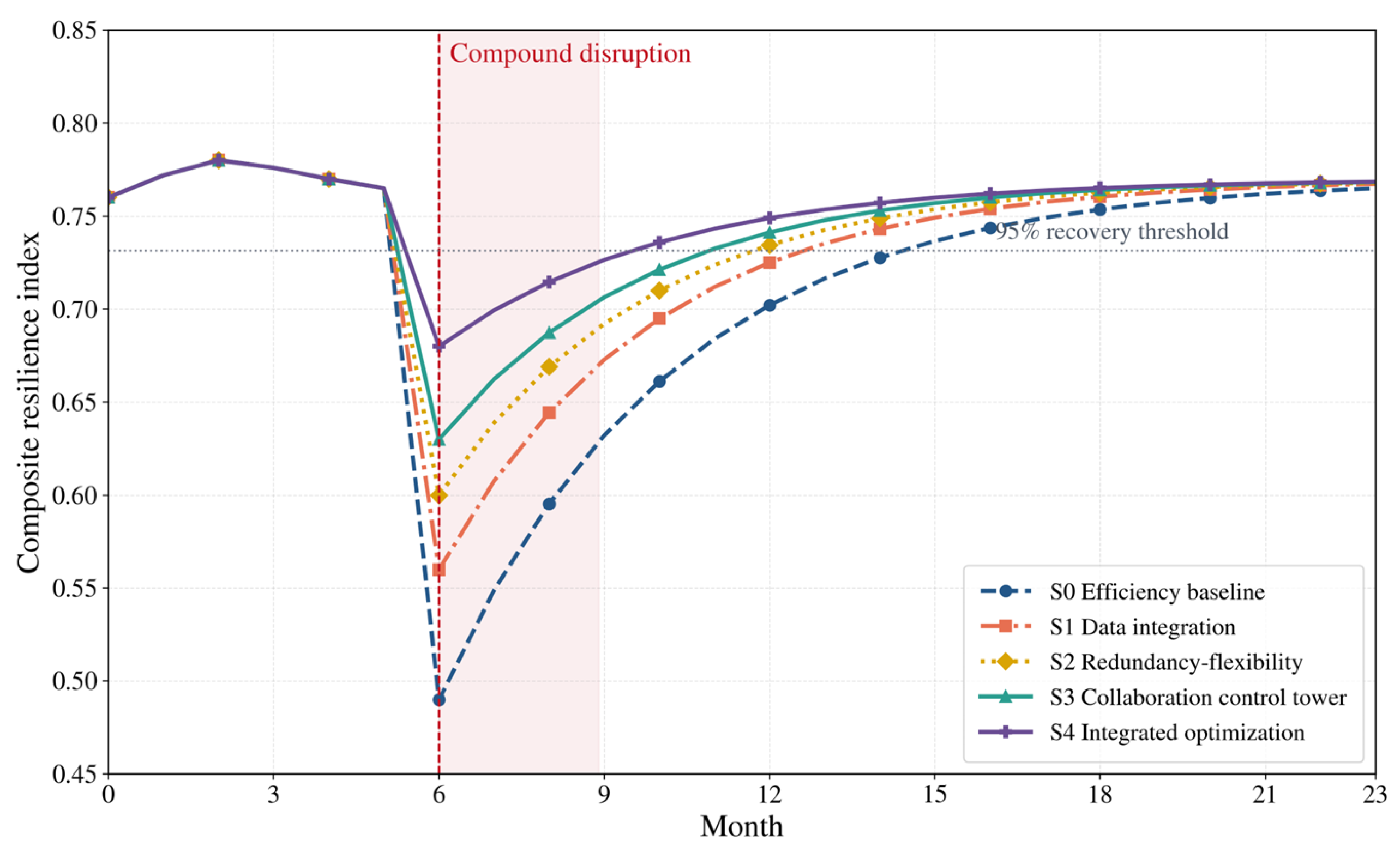
Figure 4 includes all five scenarios. S1 reduces information delay but leaves the physical absorption constraint largely unchanged. S2 produces a higher minimum through alternatives, flexible capacity, and buffer. S3 recovers faster because supplier acknowledgement and joint planning shorten coordination delay. S4 combines these mechanisms by phase and has the highest minimum and shortest TTR.

Figure 4. Dynamic resilience trajectories for S0–S4 under the compound calibration shock.

The trajectory-derived values in Table 9 replace the earlier internally inconsistent averages. Relative to S0, S4 increases minimum resilience by 38.8%, shortens TTR by 58.3%, and reduces cumulative service loss by 68.4%, at an incremental cost of 6.9%.

Table 9. Scenario results under the original mechanism-specific budgets.

Scenario	Average R	Minimum R	TTR (Months)	Cumulative Service Loss (%)	Incremental Cost (%)
S0 Efficiency baseline	0.715	0.490	8.4	9.5	0.0
S1 Data integration	0.732	0.560	6.6	6.6	3.2
S2 Redundancy-flexibility	0.740	0.600	5.7	5.3	5.6
S3 Collaboration control tower	0.745	0.630	4.9	4.3	4.8
S4 Integrated phase optimization	0.753	0.680	3.5	3.0	6.9

S4’s advantage is not explained only by its higher original cost. When every mechanism class is given the same 6.9% budget, S1–S3 improve but remain below S4 (Table 10). The minimum-resilience gap is 0.071 versus data integration, 0.049 versus redundancy-flexibility, and 0.029 versus collaboration. These gaps are smaller than in Table 9, which confirms that part—but not all—of the original advantage was resource-related.

Table 10. Equal-budget comparison at 6.9% incremental cost.

Cost-Matched Policy	Average R	Minimum R	TTR (Months)	Service Loss (%)	Cost (%)
S1 Data integration	0.738	0.609	5.4	5.6	6.9
S2 Redundancy-flexibility	0.746	0.631	4.9	4.7	6.9
S3 Collaboration control tower	0.751	0.651	4.3	3.9	6.9
S4 Integrated phase optimization	0.753	0.680	3.5	3.0	6.9

5.4. Dynamic Policy Schedule and Objective Preferences

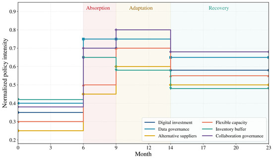
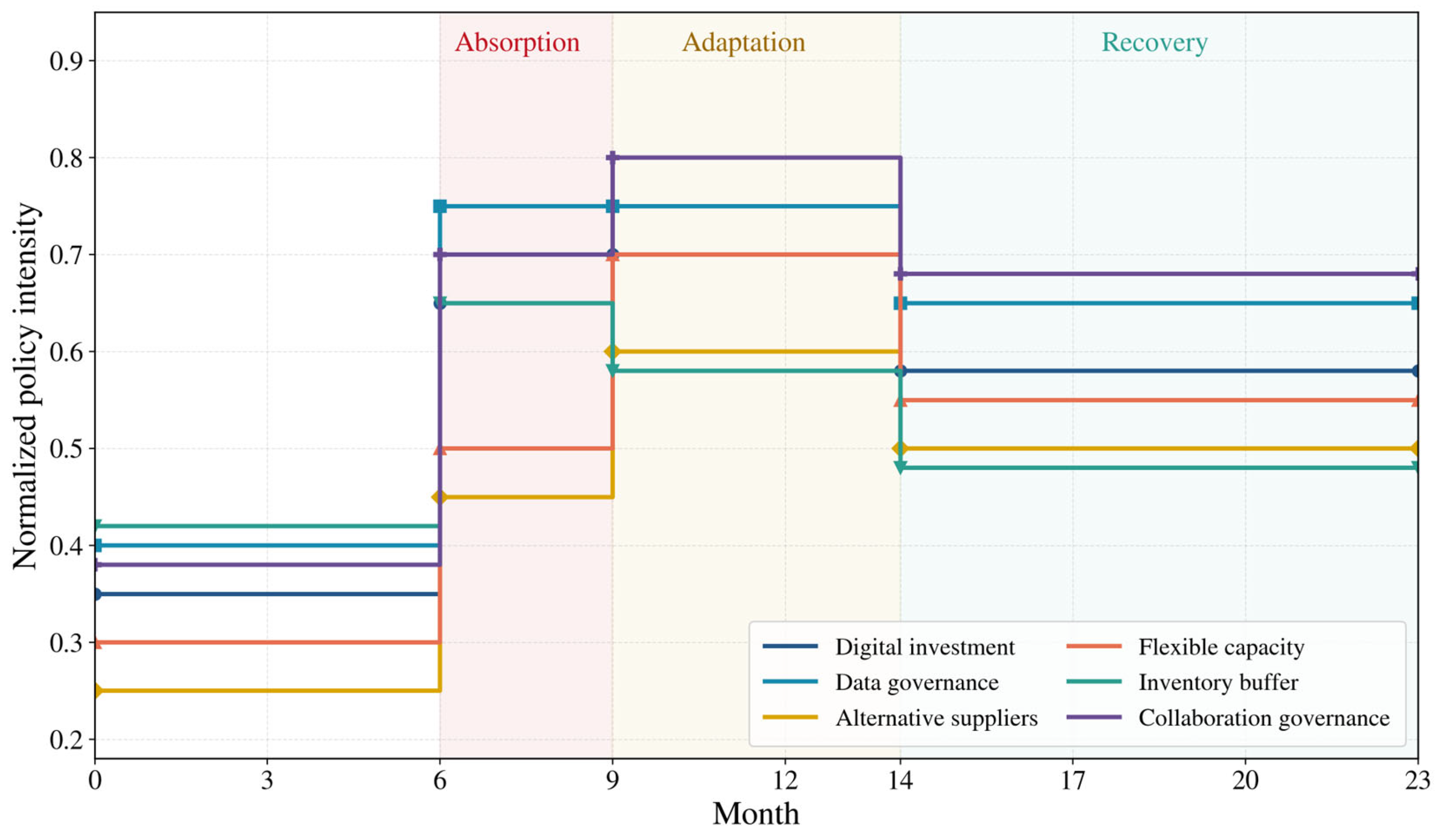
The optimized values are not a single fixed vector. Figure 5 and Table 11 show how the schedule changes. The absorption phase raises data governance, inventory buffer, and collaboration to prevent an abrupt service loss. Adaptation shifts the highest intensity to collaboration governance and flexible capacity. Recovery reduces buffer and alternative-supplier intensity while maintaining data governance and response routines. This phase structure justifies the term phase-based optimization more precisely than the original fixed settings.

Figure 5. Phase-specific policy intensities selected by the balanced constrained search.

Table 11. Phase-specific balanced policy schedule.

Policy Lever	Normal 0–6	Absorption 6–9	Adaptation 9–14	Recovery 14–24	Operational Interpretation
Digital investment	0.35	0.65	0.70	0.58	Accelerate integration, then retain critical interfaces
Data-quality governance	0.40	0.75	0.75	0.65	Increase reconciliation and update discipline
Alternative suppliers	0.25	0.45	0.60	0.50	Qualify substitutes for bottleneck components
Flexible capacity	0.30	0.50	0.70	0.55	Reconfigure bottleneck operations during adaptation
Inventory buffer	0.42	0.65	0.58	0.48	Absorb the initial shock, then release excess stock
Collaboration governance	0.38	0.70	0.80	0.68	Assign response authority and joint decision routines

Objective preferences change the portfolio, as expected (Table 12). A continuity-priority profile increases minimum resilience to 0.692 at the budget ceiling; a recovery-speed profile reaches TTR 3.1 months but a lower minimum of 0.671; and a cost-priority profile spends 5.2% but lowers minimum resilience to 0.648. The balanced result is therefore a transparent compromise, not a uniquely optimal managerial choice.

Table 12. Sensitivity to objective-function priorities.

Preference Profile $\left({\mathit{\omega }}_1,{\mathit{\omega }}_2,{\mathit{\omega }}_3,{\mathit{\omega }}_4\right)$	Average R	Minimum R	TTR	Cost (%)
Balanced (0.30, 0.30, 0.20, 0.20)	0.753	0.680	3.5	6.9
Continuity (0.25, 0.45, 0.20, 0.10)	0.756	0.692	3.4	7.0
Recovery speed (0.20, 0.25, 0.40, 0.15)	0.750	0.671	3.1	7.0
Cost control (0.20, 0.20, 0.15, 0.45)	0.742	0.648	4.4	5.2

5.5. Robustness, Unseen Shocks, and Ablation

All results in Table 13 are computed after the parameters and S4 schedule have been frozen. The schedule remains feasible under all primary perturbations, although performance declines under stronger shocks, slower implementation, and weaker initial states. The complete-case panel and the unshrunk panel yield S4 minimum-resilience values of 0.676 and 0.663, respectively. A six-month benchmark window produces 0.669, showing that the conclusion is not dependent on the three-month median. Across 1000 parameter draws, the S4 minimum-resilience interval is 0.641–0.699 and the TTR interval is 3.1–4.6 months. These tests establish numerical and design robustness within the specified model, not real-world effect size.

Table 13. Robustness and unseen-scenario results for the fixed S4 schedule.

Test	Average R	Minimum R	TTR	Interpretation
Supplier-only unseen shock	0.761	0.710	2.4	Alternatives and collaboration dominate
Demand-only unseen shock	0.765	0.724	1.9	Buffer and flexibility dominate
Logistics-only unseen shock	0.763	0.718	2.1	Visibility and coordination dominate
Short severe compound shock	0.736	0.632	4.6	Schedule remains feasible at lower minimum
Long moderate compound shock	0.741	0.646	4.4	Persistent cost and delay reduce recovery speed
Initial stocks −10%	0.733	0.638	4.5	Outcome is sensitive to preparedness
Implementation delays +50%	0.739	0.641	4.4	Delayed action erodes early gains
No shrinkage	0.746	0.663	4.0	Reliability adjustment helps but does not determine ranking
Equal reliability coefficients	0.751	0.676	3.7	Primary conclusion is coefficient-stable

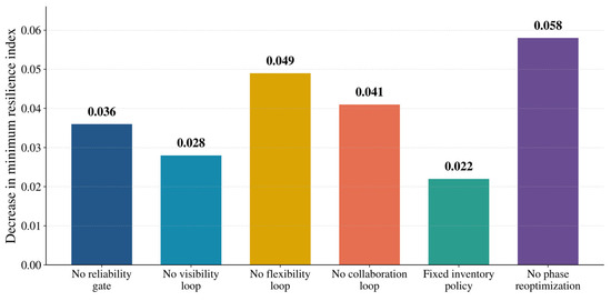
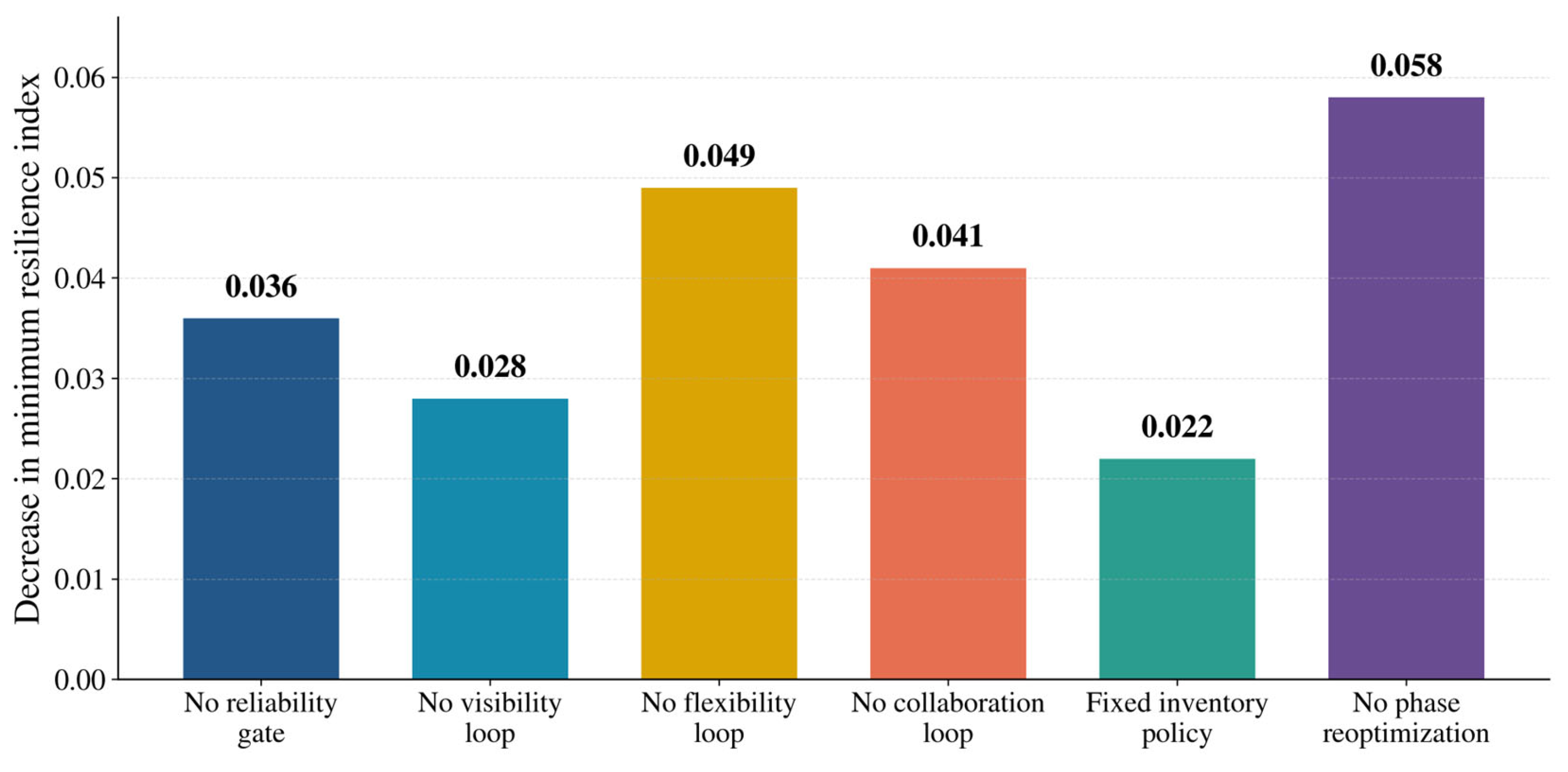
Figure 6 is aligned row-for-row with Table 14. Removing phase reoptimization causes the largest decrease in minimum resilience (0.058), followed by removing flexibility (0.049) and collaboration (0.041). Removing the reliability gate reduces minimum resilience by 0.036; this is material but smaller than the loss from eliminating operational response mechanisms.

Figure 6. Decrease in minimum resilience after removing each model component.

Table 14. Ablation results corresponding exactly to Figure 6.

Ablation	Full S4 Minimum R	Ablated Minimum R	Decrease	Ablated TTR
No reliability gate	0.680	0.644	0.036	4.1
No visibility loop	0.680	0.652	0.028	3.9
No flexibility loop	0.680	0.631	0.049	4.5
No collaboration loop	0.680	0.639	0.041	4.3
Fixed inventory policy	0.680	0.658	0.022	3.9
No phase reoptimization	0.680	0.622	0.058	4.8

5.6. Mechanism Interpretation

The experiments distinguish sensing from recoverability. S1 improves the early trajectory because higher data quality and visibility reduce recognition delay, yet its equal-budget minimum remains below S2–S4 because information cannot substitute fully for materials, qualified suppliers, or executable capacity. This is a consequence of the model’s layered structure: digital investment changes $D$ and $V$ first; $C$ and $F$ respond with delay; and service changes only when the information advantage reaches a physical or interorganizational lever.

The result should not be overstated. The positive signs linking collaboration, flexibility, buffers, and resilience were specified before simulation, based on existing theory. The experiments show the magnitude, timing, budget trade-off, and sensitivity generated by that structure. They do not independently prove that collaboration or digital investment has a causal effect in an observed firm. The empirical contribution of prior studies and the conditional simulation contribution of this study are therefore kept separate.

6. Discussion

6.1. Relation to Prior Research and Theoretical Implications

The results are consistent with empirical work showing that digitalization supports resilience through information processing, recovery capability, and inventory efficiency [6,8], but add a temporal qualification: the benefit appears only after information changes coordination or physical allocation. This qualification also complements the resource–action–performance perspective, which separates digital resources from the actions through which performance is realized [7]. In the model, digital capability is a resource stock, while collaboration governance, flexible capacity, and buffer release are actions.

The equal-budget result supports, rather than merely assumes, a configurational interpretation. Governance-fit research finds that digitally driven capability and supply chain governance work jointly [15], and the present simulation shows that a phase-based combination outperforms mechanism-specific portfolios even after expenditure is equalized. The evidence remains conditional on the model architecture and should be described as supporting or illustrating a configurational perspective, not confirming it universally.

The study differs from agent-based ripple-effect research [16]. It cannot identify which second-tier node transmits a shock, but it can show how aggregate visibility, collaboration, flexibility, and buffers accumulate and decay under delayed policies. It also differs from system-dynamics/reinforcement-learning optimization [18]. The grid search is less adaptive and may miss a continuous global optimum, but every evaluated value, constraint, and phase transition is auditable. The contribution is therefore transparent integration, not algorithmic superiority.

The reliability gate adds a measurement implication. Direct shrinkage can make a trajectory look stable by attenuating the very discontinuity that resilience research seeks to detect. Equation (5) preserves verified events and shrinks only unverified low-reliability values. The ablation and no-shrinkage tests show that this treatment improves results without determining the scenario ranking. Data quality is thus a condition for trustworthy diagnosis, not a substitute for operational capability.

6.2. Managerial Implications by Decision Owner

For senior management, the cost frontier is more useful than a single normalized optimum. Moving from a 6.9% to an 8.0% budget yields only 0.011 additional minimum resilience, whereas reducing the budget to 5.0% lowers the minimum to 0.638. The decision is therefore whether the additional 0.042 of shock-floor protection is worth 1.9 percentage points of operating cost. Senior leaders must also assign authority for supplier switching, capacity reallocation, and emergency inventory release; without that authority, the collaboration-governance control has no operational meaning.

For procurement, Table 11 does not recommend universal multi-sourcing. Alternative-supplier intensity rises most during adaptation and then declines, implying selective qualification for components with long switching lead times. Procurement should monitor RED2, AGI2, and COL2 and pre-authorize the conditions under which a substitute can be activated.

For production and logistics, the main result is phase dependence. Inventory protects the absorption phase, whereas flexible capacity has greater value during adaptation. Planners should monitor critical-material days, rescheduling cycle time, logistics delay, and the service floor. A static annual safety-stock target cannot reproduce the path shown in Figure 5.

For data and information-system teams, integration quality is operationally defined by completeness, latency, reconciliation, and predictive contribution—not by the number of installed systems. The event gate also requires an auditable disruption log. Data teams should expose both the normalized observation and its reliability components so that managers can distinguish a weak signal from a weak data feed.

For key suppliers, joint planning requires reciprocal reporting and an agreed response clock. COL1 and COL2 provide simple monitoring measures, but incentive alignment, trust, contractual rights, and the supplier’s own capacity constraints remain outside the equations. The model should therefore be embedded in a governance routine rather than treated as an automated command system.

6.3. Organizational and Behavioral Constraints

Implementation depends on decision rights and cross-functional coordination. Procurement may own supplier approval, production may own capacity changes, logistics may control routing, and finance may restrict inventory. A technically feasible schedule can fail if no role has authority to activate the relevant lever or if incentives reward local cost reduction. The framework should be paired with an escalation matrix that names the trigger, accountable owner, maximum response time, budget authority, and evidence required for each action.

Behavioral responses also matter. Suppliers may delay bad news, managers may distrust model outputs, and teams may overreact to a noisy risk score. The reliability display can reduce—but not eliminate—these problems. Training, post-event review, and documented override reasons are needed to prevent the model from becoming either an unused dashboard or an unquestioned automated prescription.

6.4. Boundary Conditions, Limitations, and Future Research

Six limitations define the strength of the evidence. First, the panel and network are generated; the study demonstrates internal reproducibility, not the behavior of a named manufacturer. Second, parameter signs and some ranges are theory- and case-design-based, so the simulation cannot be treated as independent empirical confirmation of those relationships. Third, the aggregate system-dynamics structure omits multi-tier topology, contractual substitution constraints, transport-mode choice, and financial contagion. Fourth, the two-indicator representation of each dimension is deliberately parsimonious and should be revalidated before field use. Fifth, equal entropy-CRITIC pooling is a transparent convention; alternative weights reduce but do not eliminate model dependence. Sixth, the event-preserving reliability gate depends on correct event logs and may retain false alarms or miss unlogged disruptions.

The optimization has additional limits. Policy search and numerical evaluation use the same structural model, so the study cannot claim external predictive validity. The risk of tuning to one disturbance is reduced by freezing the schedule before five unseen shock families are evaluated, but this design separation is not a substitute for prospective field validation. The deterministic grid and fixed phase boundaries may miss better continuous or state-contingent policies. The cost function uses normalized incremental-cost coefficients rather than audited cash flows. TTR is no longer double counted in the diagnostic index, but it remains both an optimization component and an evaluation outcome; this is intentional because the objective explicitly values recovery speed.

Future research should replace the generated panel with event-level records from multiple firms, estimate coefficients hierarchically, and validate the policy schedule prospectively. Multi-tier network or agent-based modules can represent propagation paths, while model predictive control can update decisions as new records arrive. Field studies should also test whether response authority, trust, incentive alignment, and cross-functional governance moderate the conversion of visibility into recovery.

7. Conclusions

The methodological result is a fully specified simulation architecture that connects an event-preserving reliability gate, a six-dimensional diagnostic index, bounded stock-flow dynamics, and phase-based constrained policy search. Inputs, state variables, diagnostic measures, and validation outcomes are separated and indicator weights, equations, parameters, constraints, search settings, and uncertainty tests are reported.

The quantitative case result is conditional on the declared compound shock and simulation assumptions. Relative to S0, S4 raises minimum resilience from 0.490 to 0.680, reduces TTR from 8.4 to 3.5 months, and lowers cumulative service loss from 9.5% to 3.0% at a 6.9% incremental cost. At the same 6.9% budget, S4 retains a minimum-resilience advantage over all mechanism-specific alternatives. Across 1000 parameter draws, its minimum-resilience interval is 0.641–0.699.

The managerial result is a sequence rather than a universal fixed setting: reliable sensing and buffer protection dominate absorption; supplier coordination and flexible capacity dominate adaptation; and selected buffers can be reduced during recovery while data and governance routines remain active. These findings suggest that digital visibility is valuable when it is connected to decision authority and executable operational levers. Because the case is generated and calibrated internally, the results should guide field testing rather than be generalized as a universal effect of digital transformation.

References

- Wieland, A.; Durach, C.F. Two perspectives on supply chain resilience. J. Bus. Logist. 2021, 42, 315–322. [Google Scholar] [CrossRef] [Scilit]
- Ivanov, D. Two views of supply chain resilience. Int. J. Prod. Res. 2024, 62, 4031–4045. [Google Scholar] [CrossRef] [Scilit]
- European Investment Bank. Navigating Supply Chain Disruptions: New Insights into the Resilience and Transformation of EU Firms; EIB: Luxembourg, 2024. [Google Scholar] [CrossRef]
- Ivanov, D.; Dolgui, A. Viability of intertwined supply networks: Extending the supply chain resilience angles towards survivability. Int. J. Prod. Res. 2020, 58, 2904–2915. [Google Scholar] [CrossRef] [Scilit]
- Ivanov, D.; Dolgui, A.; Sokolov, B. The impact of digital technology and Industry 4.0 on the ripple effect and supply chain risk analytics. Int. J. Prod. Res. 2019, 57, 829–846. [Google Scholar] [CrossRef] [Scilit]
- Zhao, N.; Hong, J.; Lau, K.H. Impact of supply chain digitalization on supply chain resilience and performance: A multi-mediation model. Int. J. Prod. Econ. 2023, 259, 108817. [Google Scholar] [CrossRef] [Scilit]
- Wu, L.; Zhang, Z.; Huang, J.; Su, I.-H.; Tian, S. Digital technologies and supply chain resilience: A resource-action-performance perspective. Inf. Syst. Front. 2025, 27, 2137–2158. [Google Scholar] [CrossRef] [Scilit]
- Tian, Y.; Cui, L. Supply chain resilience and digital transformation: Perspectives from a supply chain network. Humanit. Soc. Sci. Commun. 2025, 12, 1738. [Google Scholar] [CrossRef] [Scilit]
- Ricárdez-Estrada, J.; Garay-Rondero, C.L.; Romero, D.; Wuest, T.; Pinto, R. Identifying digital supply chain capabilities. Procedia Comput. Sci. 2024, 232, 1182–1191. [Google Scholar] [CrossRef] [Scilit]
- Xu, L.; Mak, S.; Proselkov, Y.; Brintrup, A. Towards autonomous supply chains: Definition, characteristics, conceptual framework, and autonomy levels. J. Ind. Inf. Integr. 2024, 42, 100698. [Google Scholar] [CrossRef] [Scilit]
- Nasiri, M.; Ukko, J.; Saunila, M.; Rantala, T. Managing the digital supply chain: The role of smart technologies. Technovation 2020, 96–97, 102121. [Google Scholar] [CrossRef] [Scilit]
- Zhu, S.; Song, J.; Hazen, B.T.; Lee, K.; Cegielski, C. How supply chain analytics enables operational supply chain transparency: An organizational information processing theory perspective. Int. J. Phys. Distrib. Logist. Manag. 2018, 48, 47–68. [Google Scholar] [CrossRef] [Scilit]
- Razak, G.M.; Hendry, L.C.; Stevenson, M. Supply chain traceability: A review of the benefits and its relationship with supply chain resilience. Prod. Plan. Control 2023, 34, 1114–1134. [Google Scholar] [CrossRef] [Scilit]
- Liu, Y.; Du, J.; Kang, T.; Kang, M. Establishing supply chain transparency and its impact on supply chain risk management and resilience. Oper. Manag. Res. 2024, 17, 1157–1171. [Google Scholar] [CrossRef] [Scilit]
- Lin, J.; Lin, S.; Benitez, J.; Luo, X.R.; Ajamieh, A. How to build supply chain resilience: The role of fit mechanisms between digitally-driven business capability and supply chain governance. Inf. Manag. 2023, 60, 103747. [Google Scholar] [CrossRef] [Scilit]
- Proselkov, Y.; Zhang, J.; Xu, L.; Hofmann, E.; Choi, T.Y.; Rogers, D.; Brintrup, A. Financial ripple effect in complex adaptive supply networks: An agent-based model. Int. J. Prod. Res. 2024, 62, 823–845. [Google Scholar] [CrossRef] [Scilit]
- Ivanov, D. Intelligent digital twin for supply chain stress-testing, resilience, and viability. Int. J. Prod. Econ. 2023, 263, 108938. [Google Scholar] [CrossRef] [Scilit]
- Bussieweke, F.; Mula, J.; Campuzano-Bolarin, F. Optimisation of recovery policies in the era of supply chain disruptions: A system dynamics and reinforcement learning approach. Int. J. Prod. Res. 2025, 63, 1649–1673. [Google Scholar] [CrossRef] [Scilit]
- Katsaliaki, K.; Galetsi, P.; Kumar, S. Supply chain disruptions and resilience: A major review and future research agenda. Ann. Oper. Res. 2022, 319, 965–1002. [Google Scholar] [CrossRef] [Scilit]
- Llaguno, A.; Mula, J.; Campuzano-Bolarin, F. State of the art, conceptual framework and simulation analysis of the ripple effect on supply chains. Int. J. Prod. Res. 2022, 60, 2044–2066. [Google Scholar] [CrossRef] [Scilit]
- Scholten, K.; Schilder, S. The role of collaboration in supply chain resilience. Supply Chain Manag. 2015, 20, 471–484. [Google Scholar] [CrossRef] [Scilit]
- Srinivasan, R.; Swink, M. An investigation of visibility and flexibility as complements to supply chain analytics: An organizational information processing theory perspective. Prod. Oper. Manag. 2018, 27, 1849–1867. [Google Scholar] [CrossRef] [Scilit]
- Kazancoglu, I.; Ozbiltekin-Pala, M.; Mangla, S.K.; Kazancoglu, Y.; Jabeen, F. Role of flexibility, agility and responsiveness for sustainable supply chain resilience during COVID-19. J. Clean. Prod. 2022, 362, 132431. [Google Scholar] [CrossRef] [Scilit]
- Diakoulaki, D.; Mavrotas, G.; Papayannakis, L. Determining objective weights in multiple criteria problems: The CRITIC method. Comput. Oper. Res. 1995, 22, 763–770. [Google Scholar] [CrossRef] [Scilit]
- Shannon, C.E. A mathematical theory of communication. Bell Syst. Tech. J. 1948, 27, 379–423. [Google Scholar] [CrossRef] [Scilit]
- Sterman, J.D. System dynamics modeling: Tools for learning in a complex world. Calif. Manag. Rev. 2001, 43, 8–25. [Google Scholar] [CrossRef] [Scilit]
- Ivanov, D. Predicting the impacts of epidemic outbreaks on global supply chains: A simulation-based analysis on the example of coronavirus. Transp. Res. Part E Logist. Transp. Rev. 2020, 136, 101922. [Google Scholar] [CrossRef] [Scilit]
- Qader, G.; Junaid, M.; Abbas, Q.; Mubarik, M.S. Industry 4.0 enables supply chain resilience and supply chain performance. Technol. Forecast. Soc. Change 2022, 185, 122026. [Google Scholar] [CrossRef] [Scilit]
- Zamani, E.D.; Smyth, C.; Gupta, S.; Dennehy, D. Artificial intelligence and big data analytics for supply chain resilience: A systematic literature review. Ann. Oper. Res. 2023, 327, 605–632. [Google Scholar] [CrossRef] [Scilit]
- Shi, Y.; Zheng, X.; Venkatesh, V.G.; Humdan, E.A.; Paul, S.K. The impact of digitalization on supply chain resilience: An empirical study of the Chinese manufacturing industry. J. Bus. Ind. Mark. 2023, 38, 1–11. [Google Scholar] [CrossRef] [Scilit]
- Harju, A.; Hallikas, J.; Immonen, M.; Lintukangas, K. The impact of procurement digitalization on supply chain resilience: Empirical evidence from Finland. Supply Chain Manag. 2023, 28, 62–76. [Google Scholar] [CrossRef] [Scilit]
- Sodhi, M.S.; Seyedghorban, Z.; Tahernejad, H.; Samson, D. Why emerging supply chain technologies initially disappoint: Blockchain, IoT, and AI. Prod. Oper. Manag. 2022, 31, 2517–2537. [Google Scholar] [CrossRef] [Scilit]
- Christopher, M.; Peck, H. Building the resilient supply chain. Int. J. Logist. Manag. 2004, 15, 1–13. [Google Scholar] [CrossRef] [Scilit]
- Tang, C.S. Perspectives in supply chain risk management. Int. J. Prod. Econ. 2006, 103, 451–488. [Google Scholar] [CrossRef] [Scilit]
- Golan, M.S.; Jernegan, L.H.; Linkov, I. Trends and applications of resilience analytics in supply chain modeling: Systematic literature review. Environ. Syst. Decis. 2020, 40, 222–243. [Google Scholar] [CrossRef] [Scilit]
- Hosseini, S.; Ivanov, D.; Dolgui, A. Review of quantitative methods for supply chain resilience analysis. Transp. Res. Part E Logist. Transp. Rev. 2019, 125, 285–307. [Google Scholar] [CrossRef] [Scilit]
- Qi, R.; Ma, G.; Liu, C.; Zhang, Q.; Wang, Q. Enterprise digital transformation and supply chain resilience. Financ. Res. Lett. 2024, 66, 105564. [Google Scholar] [CrossRef] [Scilit]
- Ge, R.; Bao, H. Digital transformation and resilience of supply chain in manufacture listed firms: A backward spillover effects in the vertical supply chain relationship. Financ. Res. Lett. 2024, 65, 105516. [Google Scholar] [CrossRef] [Scilit]
- Jia, L.; Li, J. How does digital collaboration impact supply chain resilience. Financ. Res. Lett. 2024, 66, 105684. [Google Scholar] [CrossRef] [Scilit]
- Zhang, J.; Miao, X.; Shang, T. Impact mechanism of digital transformation on supply chain resilience. Financ. Res. Lett. 2025, 76, 106993. [Google Scholar] [CrossRef] [Scilit]
- Hossain, M.I.; Talapatra, S.; Saha, P.; Belal, H.M. From theory to practice: Leveraging digital twin technologies and supply chain disruption mitigation strategies for enhanced supply chain resilience with strategic fit in focus. Glob. J. Flex. Syst. Manag. 2025, 26, 87–109. [Google Scholar] [CrossRef] [Scilit]
- Corsini, R.R.; Costa, A.; Fichera, S.; Framiñan, J.M. Digital twin model with machine learning and optimization for resilient production-distribution systems under disruptions. Comput. Ind. Eng. 2024, 191, 110145. [Google Scholar] [CrossRef] [Scilit]
- Malekzadeh, M.; Torabi, S.A.; Sheikhalishahi, M. A supply chain digital twin for resilience analysis under immediate and long-term disruptions: A case study in plastic parts’ manufacturing. Int. J. Prod. Res. 2025, 63, 10445–10467. [Google Scholar] [CrossRef] [Scilit]
Disclaimer/Publisher’s Note: The statements, opinions and data contained in all publications are solely those of the individual author(s) and contributor(s) and not of MDPI and/or the editor(s). MDPI and/or the editor(s) disclaim responsibility for any injury to people or property resulting from any ideas, methods, instructions or products referred to in the content. |
© 2026 by the authors. Licensee MDPI, Basel, Switzerland. This article is an open access article distributed under the terms and conditions of the Creative Commons Attribution (CC BY) license.