


Abstract
This study examines agricultural greenhouse-gas (GHG) emission scale and source composition across a fixed EU-27 geographical cohort and Mercosur-4 (Argentina, Brazil, Paraguay, and Uruguay) over 2002–2023. Using FAOSTAT emissions totals, a balanced nine-source profile is constructed for 31 countries (682 country-year observations). Hellinger and Aitchison distances, Kendall–Theil–Sen trends, Ward.D2 clustering, PERMANOVA/PERMDISP, and sensitivity analyses distinguish aggregate emission-weighted profiles from equal-country profiles. Common9 emissions declined by 10.0% in the EU-27 but increased by 26.1% in Mercosur-4. The emission-weighted inter-bloc Hellinger distance showed no statistically supported trend (tau = −0.177, p = 0.248), whereas the equal-country distance declined by 4.5% (tau = −0.688, p < 0.001). CoDA6 Aitchison distance declined by 5.2% (tau = −0.610, p < 0.001), but this result concerns a distinct six-part strictly positive subcomposition rather than confirming Primary9 convergence. EU within-bloc dispersion increased by 6.4%. Two recent Primary9 EU regimes are identified, but their partition is sensitive to drained organic soils. The study therefore finds scale divergence and estimand-specific partial compositional convergence, providing a pre-application, non-causal baseline for post-2026 monitoring. Conditional inclusion of rice under a stated zero-fill assumption preserves the contrasting weighted and equal-country trends; absolute-share-gap diagnostics qualify the geometry-dependent contribution of drained organic soils.
1. Introduction
Agriculture is central to climate mitigation because greenhouse-gas (GHG) emissions arise from heterogeneous livestock, soil, nutrient-management and land-use processes that cannot be represented adequately by a single aggregate indicator. Nabuurs et al. [1] emphasise that agriculture, forestry, and other land use (AFOLU) involves source- and context-specific mitigation challenges, while Dace and Blumberga [2] show that assessments of EU agricultural GHG performance depend materially on the indicator used. A decline in total emissions therefore need not imply convergence in emission composition, emission intensity, or heterogeneity across countries. This distinction motivates a separate analysis of the scale of emissions and their source composition.
In the EU, agricultural emissions declined substantially before 2010 but subsequently stagnated despite substantial climate-related Common Agricultural Policy expenditure [3], while more recent evidence indicates that reductions depend on national policy mixes [4]. Mercosur is not homogeneous. Brazil’s pasture-based cattle systems make enteric methane especially prominent [5], but official inventories also show distinct national structures. Paraguay’s agriculture-and-livestock inventory is dominated by enteric fermentation and agricultural soils [6], while Uruguay reports enteric CH4 and managed-soil N2O as its principal AFOLU emission sources, with rice methane playing a smaller role [7]. Argentina’s national inventory separately reports agriculture, livestock, forestry, and other land uses and continually updates livestock parameters across production regions [8]. The Mercosur-4 comparison therefore treats Argentina, Brazil, Paraguay, and Uruguay separately rather than using Brazilian evidence as representative of the bloc.
These differences are increasingly relevant in the context of EU-Mercosur economic integration. Mercosur was established in 1991 by Argentina, Brazil, Paraguay, and Uruguay, the four countries included here as Mercosur-4. Interregional cooperation with the European Union was formalised through the 1995 Framework Cooperation Agreement, and negotiations toward a broader association and trade agreement intensified from 1999 onward [9]. After repeated interruptions, the parties announced an agreement in principle in June 2019 [9].
The partnership agreement was politically concluded in December 2024 [10], and the EU–Mercosur Partnership Agreement and Interim Trade Agreement were signed on 17 January 2026; provisional application of the Interim Trade Agreement began on 1 May 2026 [11]. The 2002–2023 period therefore provides a pre-application window in which structural change can be examined without attributing historical trends to the agreement.
The environmental implications of the agreement remain contested. Prospective studies indicate that liberalisation may affect deforestation, land-use transitions, and associated GHG emissions, although magnitudes depend on production responses, governance, and modelling assumptions [12,13]. Cesar de Oliveira et al. [14] argue that the agreement may also support environmental cooperation and land-use governance, while Hagemejer et al. [15] emphasise its interaction with an evolving EU sustainability framework.
Institutional studies identify further challenges involving sustainability assessment, environmental enforcement, deforestation, and divergent expectations between the blocs [9,16,17]. Del Pupo [18] and Gosselin et al. [10] show that trade, agriculture, and environmental protection have become closely interconnected in the agreement’s political trajectory. However, this literature is primarily prospective, regulatory, or land-use oriented and does not jointly establish how agricultural GHG source structures differed and evolved across the EU-27 and Mercosur-4 before application.
Accordingly, the central research question is as follows: How did the scale and source composition of agricultural GHG emissions differ and evolve between the EU-27 and Mercosur-4 over 2002–2023, and to what extent did these trajectories indicate inter-bloc or within-bloc structural convergence?
The objective is to construct a harmonised country-level pre-application benchmark that separates emission scale from source composition and identifies where structural similarities and asymmetries are located. Using FAOSTAT emissions totals for a balanced panel of 31 countries and a common nine-source profile, the study combines emission-weighted and equal-country compositions with Hellinger and Aitchison distances, trend analysis, clustering and validation, within-bloc pairwise dispersion, PERMANOVA/PERMDISP, source decomposition, and sensitivity tests. These estimands are deliberately kept separate; the emission-weighted profile represents the aggregate bloc structure, the equal-country profile represents the arithmetic mean national composition, and CoDA6 evaluates a distinct strictly positive six-part subcomposition.
Four confirmatory hypotheses and one exploratory decomposition question organise the analysis. H1 tests whether recent (2020–2023) EU-27 and Mercosur-4 source compositions occupy different regions of compositional space, with PERMDISP used to qualify PERMANOVA interpretation. H2 tests whether inter-bloc structural distance declined over 2002–2023. H3 tests whether the fixed EU-27 geographical cohort forms distinct and stable recent Primary9 regimes. H4 tests whether within-EU structural dispersion declined over time, corresponding to compositional sigma-convergence. The former H5 is recast as an exploratory decomposition question (E1): which sources account for the observed recent EU-Mercosur structural distance? No ex ante threshold for a ‘limited set’ or ‘most’ is imposed.
The contribution is empirical and methodological. The study separates emission scale from composition, distinguishes emission-weighted from equal-country bloc profiles, tests inter-bloc and within-EU convergence, identifies recent EU Primary9 regimes, and decomposes the residual EU-Mercosur distance by source. It therefore avoids treating convergence in per-capita emissions, absolute emissions, emission intensity, sigma-dispersion, and source composition as interchangeable concepts. Because the empirical period predates provisional application of the Interim Trade Agreement, the study does not estimate trade-policy effects; it provides a reproducible baseline for later post-application evaluation.
The article is organised into six sections. Following the Introduction, Section 2 reviews the relevant literature and develops the hypotheses. Section 3 presents the data and methods, Section 4 reports the empirical results, Section 5 discusses the findings and their limitations, and Section 6 concludes with policy implications and directions for future research.
2. Literature Review
Agricultural GHG performance is multidimensional because changes in aggregate emissions need not coincide with changes in emission intensity, source composition, or heterogeneity across countries. The broader emissions-convergence literature typically evaluates convergence in levels, per-capita values, or intensities. Strazicich and List [19], for example, tested the stochastic and conditional convergence of CO2 emission levels across industrial countries, while Aldy [20] studied the international distribution of per-capita CO2 emissions. These concepts differ from the present study’s compositional question. Here, convergence means declining distance between vectors of relative source shares; it can occur even when total emissions diverge. Likewise, sigma-convergence refers here to declining dispersion among country source compositions, not declining dispersion in per-capita emission levels.
Compositional analysis requires attention to relative information and to the unit-sum constraint. Aitchison [21] established the log-ratio geometry for strictly positive compositions, and Pawlowsky-Glahn et al. [22] provide the subsequent framework for interpreting ratios, subcompositions, centres, and distances. Accordingly, Hellinger distance is used for the nine-part non-negative Primary9 composition, whereas Aitchison distance is used only for the strictly positive CoDA6 subcomposition. Convergence under CoDA6 therefore concerns a different estimand and cannot be treated as confirmation of convergence under Primary9.
The analytical boundary also requires care. FAOSTAT drained-organic-soil emissions arise from drained cropland and grazed grassland organic soils and are reported using land-use-based activity data and IPCC emission factors [23]. National inventory research likewise shows that drained organic soils are often accounted for within AFOLU/LULUCF frameworks rather than as a conventional direct agricultural source [24]. They are retained here because the present study follows a harmonised FAOSTAT source bundle and because agricultural drainage of cropland and grassland is directly relevant to farmed land. Their inclusion is nevertheless treated as a boundary choice and tested explicitly by source omission. Deforestation and net forest conversion are excluded because they are separate land-use-change categories outside the harmonised Primary9 bundle and would change the estimand from an agriculture-related source profile toward a broader AFOLU inventory. Published external validation directly compares the FAOSTAT drained-organic-soil methodology with official UNFCCC country submissions. Conchedda and Tubiello [25] used 2017 data from the 2019 National Greenhouse Gas Inventories for 38 Annex I Parties and reported that FAOSTAT estimates explained about 60% of the cross-country variability in official country-reported data. This provides an independent country-level inventory cross-check for the harmonised FAOSTAT series, while exact equality is not expected because national inventories may use country-specific activity data, emission factors, and sectoral allocations.
The EU literature also provides reasons to expect internal emission regimes rather than a single common pathway. Dace and Blumberga [2] document substantial interstate variation, Mohammed et al. [26] report country-specific emission-agriculture relationships, and Stetter et al. [4] show heterogeneous outcomes from different policy mixes. These studies motivate multivariate classification of source profiles, but clustering and sigma-convergence answer different questions; clustering describes configurations in a chosen compositional space, whereas sigma-convergence asks whether pairwise structural distances shrink over time. A stable partition can therefore coexist with rising dispersion. Verschuuren [27] likewise emphasises that agricultural GHG mitigation options depend on the regulatory and sectoral context.
A separate literature examines the environmental implications of EU–Mercosur trade. Arima et al. [12] and Mercado Cordova and Koo [13] use prospective modelling to show that liberalisation may affect deforestation, land-use transitions, and associated GHG emissions, with outcomes depending on production responses and land-use assumptions. Mroczek et al. [28] further show that EU–South America beef-trade implications depend on production and market structures, reinforcing the relevance of livestock composition to the agreement.
Complementary empirical work by Koengkan and co-authors provides additional context for the environmental dynamics of Mercosur and agriculture. Koengkan [29] found that renewable-energy consumption reduced CO2 emissions in Mercosur over 1980–2014, although the effect was modest and fossil-fuel dependence remained high. Koengkan et al. [30] documented bidirectional links among CO2 emissions, renewable and non-renewable energy use, and economic growth in the Southern Common Market, while Karimi Alavijeh et al. [31] found that agricultural value added was positively associated with CO2 emissions across major developing economies, particularly at higher emission quantiles. Together, these studies reinforce the need to distinguish aggregate emission drivers from the source-composition dynamics examined here.
Cesar de Oliveira et al. [14] argue that the agreement can provide a platform for environmental cooperation and land-use governance, although it cannot eliminate conversion risks by itself. Hagemejer et al. [15] likewise stress that sustainability effects are conditional and interact with an evolving EU regulatory environment. These contributions are important for assessing potential agreement effects, but their emphasis is prospective, scenario-based, regulatory, or land-use oriented rather than a harmonised historical comparison of agricultural emission-source structures before application.
Institutional research reinforces the need for a baseline. Harrison and Paulini [16] question whether Sustainability Impact Assessments and Trade and Sustainable Development chapters adequately integrate trade, environmental, and developmental objectives. Palmieri et al. [9] identify deforestation, pesticides, and divergent sustainability expectations as central sources of contestation, while Olech et al. [17] show how disagreement between environmental indicators can weaken enforcement.
Del Pupo [18] demonstrates that sustainability has become a strategic terrain in the politicisation of agricultural liberalisation, and Gosselin et al. [10] conceptualise the interaction among trade, agriculture, and environmental protection as a three-body problem that can generate persistent policy instability. Consequently, post-implementation environmental performance cannot be interpreted credibly if the scale of emissions, source composition, national heterogeneity, and broader land-use change are conflated.
Taken together, the literature leaves a specific empirical gap: a long-run, harmonised, country-level pre-application comparison of EU-27 and Mercosur-4 agricultural GHG source structures that separates scale from composition, distinguishes aggregate emission-weighted from representative equal-country profiles, tests estimand-specific convergence, evaluates within-EU dispersion, and decomposes the remaining structural distance by source. The unresolved issue is therefore not simply whether agricultural GHG totals change, but whether relative source structures become more similar and under which weighting and compositional boundary.
Figure 1 synthesises the literature, empirical gap, and analytical questions. H1–H4 are confirmatory hypotheses, while E1 is an exploratory decomposition objective.
Figure 1.
Literature synthesis, empirical gap, and analytical framework for EU–Mercosur agricultural GHG emission structures. H1–H4 are confirmatory hypotheses, while E1 is the exploratory objective identifying which sources account for the recent EU–Mercosur structural distance. The author created this figure using ChatGPT (OpenAI, GPT-5.6 Sol).
Accordingly, the study tests H1, whether recent 2020–2023 EU-27 and Mercosur-4 source compositions differ in multivariate compositional space; H2, whether inter-bloc structural distance declines over 2002–2023; H3, whether EU-27 countries form distinct and stable recent Primary9 regimes; and H4, whether within-EU structural dispersion declines over time. An exploratory objective (E1) examines which sources account for the recent EU–Mercosur structural distance. E1 is treated as exploratory because no ex ante threshold was specified to define how many sources would constitute a “limited set” or what share of the total distance would constitute “most.”
3. Materials and Methods
This section describes the data, sample construction, variables, and statistical methods used to analyse agricultural GHG emission structures across the fixed EU-27 geographical cohort and Mercosur-4 during 2002–2023. Detailed robustness and diagnostic outputs are reported in Appendix A Table A1, Table A2, Table A3, Table A4, Table A5, Table A6 and Table A7 and Figure A1 and Supplementary Tables S1–S21 and Figures S1–S3. All statistical analyses were conducted using R version 4.6.1 within the RStudio 2026.07.0 integrated development environment.
3.1. Materials
The analytical comparison uses a fixed EU-27 geographical cohort comprising Austria, Belgium, Bulgaria, Croatia, Cyprus, Czechia, Denmark, Estonia, Finland, France, Germany, Greece, Hungary, Ireland, Italy, Latvia, Lithuania, Luxembourg, Malta, the Netherlands, Poland, Portugal, Romania, Slovakia, Slovenia, Spain, and Sweden, together with Argentina, Brazil, Paraguay, and Uruguay (Mercosur-4). The cohort is held constant for comparability; it does not imply common institutional membership throughout 2002–2023. Several current EU-27 countries joined after 2002, while the United Kingdom was an EU member until 2020 but is not part of the fixed EU-27 geographical cohort analysed here. The geographical coverage of the countries included in the analysis is shown in Figure 2 below.
Figure 2.
Geographical coverage of the fixed analytical cohort: the current EU-27 geographical set and Mercosur-4 (Argentina, Brazil, Paraguay and Uruguay). The geographical sample is held constant for the period 2002–2023 and should not be read as contemporaneous institutional membership in every year. EU, European Union; Mercosur, Southern Common Market (Mercado Común del Sur). The author created this figure using R 4.6.1 in RStudio 2026.07.0.
Mercosur-4 contains the four South American counterparties used in the historical EU-Mercosur comparison and in the agreement analysed here: Argentina, Brazil, Paraguay, and Uruguay, as shown in Figure 2, above. Bolivia is not included in the empirical sample; its later accession to Mercosur does not alter the fixed four-country historical cohort used for 2002–2023. Venezuela is also absent from the analysis [11,32].
The analysis covers 2002–2023 as a balanced panel of 31 countries over 22 years (682 country-year observations). The starting year is empirical rather than institutional; the coverage assessment in Table S1 shows that 2002 is the earliest year from which nine common source categories are simultaneously complete for both blocs through 2023. Earlier candidate windows provide only eight common complete categories. The choice therefore avoids interpolation, source switching, and time-varying analytical boundaries.
Annual trends, structural distance, concentration, and within-bloc dispersion use the full 2002–2023 period. Four-year averages for 2002–2005 and 2020–2023 are used only to assess long-run structural change and recent country- and bloc-level profiles.
Temporal regime persistence uses non-overlapping windows (2002–2005, 2006–2009, 2010–2013, 2014–2017, 2018–2020, and 2021–2023). The final two windows contain three rather than four years because the 22-year sample does not divide evenly into four-year blocks. Their averaged profiles therefore need not have the same sampling variability as the four-year profiles; ARI comparisons are interpreted as descriptive stability diagnostics rather than estimates with identical precision.
Table S1 reports the balanced-window assessment; Table A1 documents source coverage, explicit zeros, and analytical inclusion.
3.1.1. Data Source and Greenhouse-Gas Accounting
Annual emissions for every country, year and retained source are drawn from the same FAOSTAT emissions totals (GT) domain, element ‘Emissions (CO2eq) (AR5)’, in kilotonnes of CO2 equivalent (kt CO2eq). The FAOSTAT dataset provides complete observations for all nine Primary9 emission sources across the 31 countries during 2002–2023, yielding a balanced panel of 682 country-year observations. The series applies 100-year IPCC AR5 global-warming potentials and FAOSTAT Tier 1 estimates [23]. The analysis therefore compares harmonised national estimates rather than direct farm measurements or country-submitted inventory values.
The initial source universe comprises eleven FAOSTAT categories: enteric fermentation, manure management, rice cultivation, synthetic fertilisers, manure applied to soils, manure left on pasture, crop residues, burning of crop residues, on-farm energy use, drained organic soils, and savanna fires. The boundary deliberately combines conventional agricultural sources with selected agriculture-related land sources. Drained organic soils represent emissions associated with drained cropland and grazed grassland organic soils [23,24]; savanna fires represent FAOSTAT biomass-fire emissions from savanna/grassland-type vegetation rather than deforestation [23]. Forest land, net forest conversion/deforestation, and broader land-use change are excluded because they are separate FAOSTAT/AFOLU categories and would define a broader land-use estimand. This asymmetry is therefore a stated boundary choice, not an assertion that drained organic soils are a direct agricultural process identical to enteric fermentation or fertiliser use.
3.1.2. Variable Construction and Analytical Sets
Table 1 defines the emission-source variables, derived indicators, and analytical specifications used throughout this study.
Table 1.
Definition, measurement, and analytical role of variables.
Primary9 contains nine sources with complete common coverage: enteric fermentation, manure management, synthetic fertilisers, manure applied to soils, manure left on pasture, crop residues, burning of crop residues, drained organic soils, and savanna fires. Rice cultivation is excluded from the complete-case Primary9 inter-bloc comparison because the FAOSTAT EU-27 series has 176 of 594 rice records (29.6%), corresponding to eight complete 22-year country series, whereas Mercosur-4 has 88 of 88 records. The remaining 418 EU country-year combinations have no reported rice-emission values; their status as structural zeros cannot be confirmed from the available emissions data. On-farm energy use is excluded because Mercosur coverage is 66 of 88 cells, reflecting the absence of a continuous series for Paraguay.
Rice and on-farm energy are retained in the original bloc-specific ten-source analyses. A separate assumption-based inter-bloc Rice10-Z sensitivity, reported in Table A7, assigns zero only to the 418 unreported EU rice cells and leaves the Primary9 baseline unchanged.
The eight EU rice-reporting countries are Bulgaria, France, Greece, Hungary, Italy, Portugal, Romania, and Spain, each with 22 positive entries during 2002–2023. All 19 other EU countries have 22 unreported rice-emission cells each; none of the 176 reported EU rice values is an explicit zero. Independently, Eurostat reports that rice was cultivated in eight EU Member States in both 2022 and 2023 [33,34]. This supports the plausibility of non-production in the two recent years but does not validate all 418 historical country-year blanks. Consequently, Rice10-Z is an explicitly conditional zero-imputation sensitivity, not a reclassification of missing observations as verified structural zeros (see Table A7).
Primary9 retains explicit reported zeros in the FAOSTAT dataset; missing records are not recoded to zero. For drained organic soils, the 22 Mercosur zero observations are all Paraguay (2002–2023), while the EU has 22 zeros for Cyprus and 22 for Malta. These are dataset zeros rather than missing cells. The present materials do not establish whether each represents a biophysical absence or a reporting/modelled zero; so, no stronger interpretation is imposed. Hellinger geometry accommodates these zeros without pseudocounts. CoDA6 is instead restricted to six sources that are strictly positive in every country-year observation: enteric fermentation, manure management, synthetic fertilisers, manure applied to soils, manure left on pasture, and crop residues.
Emissions are not normalised by agricultural area, output, or livestock units because the study compares the scale and composition of the harmonised emissions bundle rather than productive emission intensity. Intensity analysis requires additional denominators and measurement assumptions [2]. Common9 emissions and compositional shares are therefore reported in parallel, so that greater compositional similarity is not conflated with lower emissions.
For source i, country c and year t, the within-country source share is shown in Equation (1):
where is the share of emission source in country and year , is the corresponding emission level in kt CO2eq, and indexes the Primary9 source categories. The harmonised nine-source scale measure is defined in Equation (2):
where denotes the Common9 emission scale for country in year , expressed in kt CO2eq, and denotes emissions from Primary9 source . is the sum of the nine harmonised source categories and is used for consistent cross-country and inter-bloc scale comparisons; it does not represent total national agricultural GHG emissions.
3.2. Methods
3.2.1. Descriptive, Concentration and Compositional Measures
Descriptive statistics include country-year observations, mean, standard deviation, median, interquartile range, minimum, maximum, mean country-year source share, and emission-weighted source share; medians and interquartile ranges complement means and standard deviations given heterogeneity in national emission levels. Source concentration and diversity are measured using the Herfindahl–Hirschman Index (HHI) and Shannon index from Primary9 shares [35,36,37], with HHI defined in Equation (3):
where is the Herfindahl-Hirschman concentration index for country in year , and is the share of source , with indexing the Primary9 categories. Higher HHI values indicate greater concentration across fewer sources. The complementary Shannon diversity measure is defined in Equation (4):
where is the Shannon diversity index for country in year , is the share of source , and
denotes the natural logarithm, with for zero shares. Higher values indicate a more even source distribution, whereas higher HHI values indicate greater concentration. Annual country-level estimates are reported in Table S3, with bloc-specific ten-source robustness in Table S8. Two bloc-level compositions are distinguished; the emission-weighted specification gives greater influence to larger national emitters, as defined in Equation (5):
where is the emission-weighted share of source in bloc and year , and is the corresponding emission level for country . The denominator is total Common9 emissions across all countries in bloc , so that larger emitters receive greater weight. The equal-country composition instead averages country-level source shares across the countries, as defined in Equation (6):
where the equal-country share is calculated as the arithmetic mean of the country-level source-share vectors within bloc and year . Each country therefore receives an equal weight of , irrespective of its emission scale. This measure is an arithmetic mean in share space, not the Aitchison compositional centre, which is based on geometric means in log-ratio geometry. The emission-weighted composition represents the aggregate bloc profile, whereas the equal-country composition represents the average national source profile. Accordingly, convergence in one estimand does not imply convergence in the other.
3.2.2. Structural Distances, Within-Bloc Dispersion and Source Decomposition
The primary non-negative geometry uses Hellinger distance applied to Primary9 source shares. The square-root transformation allows genuine zeros without pseudocount replacement [38]. This geometry is used for Primary9 inter-bloc distances, country-level pairwise distances, within-bloc dispersion, Primary9 PERMANOVA/PERMDISP, and the squared-Hellinger source decomposition. EU Ward.D2 clustering uses Euclidean distance after the same square-root transformation, which is proportional to Hellinger geometry up to a constant scaling. CoDA6 analyses use a different log-ratio/Aitchison geometry and are interpreted as a distinct subcompositional estimand. The Hellinger distance used throughout the Primary9 analyses is defined in Equation (7):
where denotes the Hellinger distance between source-share compositions and , and and are the corresponding shares of source . With the normalisation, , where 0 indicates identical profiles and 1 maximal separation.
The same geometry is used for country-level structural change, Mercosur pairwise comparisons, annual inter-bloc distances, and within-bloc dispersion. Because is insufficient for a stable Mercosur regime taxonomy, clustering is not applied; all six recent-period pairwise distances are reported in Table S5. Within-bloc structural dispersion is defined as the mean pairwise country distance within each bloc-year, as shown in Equation (8):
where denotes within-bloc structural dispersion for bloc in year , is the number of countries in the bloc, and is the Hellinger distance between the source-share compositions of countries and . Higher values indicate greater cross-country compositional heterogeneity. A decline in is interpreted as evidence consistent with compositional -convergence, whereas an increase indicates compositional -divergence. As an additional cross-bloc robustness diagnostic, the analysis calculates the annual mean Hellinger distance across all 27 × 4 = 108 EU–Mercosur country pairs. This measure differs from both the emission-weighted bloc distance and the distance between equal-country bloc profiles because pairwise distances are calculated at the country level and then averaged, rather than constructing bloc-level compositions before measuring distance. The resulting annual series is reported in Table S20. To identify the individual source contributions to the structural separation between two compositions, the squared-Hellinger distance is further decomposed by source, as defined in Equation (9):
where is the percentage contribution of source to the squared-Hellinger distance, and and are the corresponding source shares in the two compositions. Contributions sum to 100% within each period and weighting scheme and represent contributions to structural distance, not causal emission effects. Annual source-share gaps are reported in Table S7, and the recent-period decomposition is shown in Figure S2.
For each source i with shares p_i and q_i, its squared-Hellinger numerator is (√p_i − √q_i)2 = (p_i − q_i)2/(√p_i + √q_i)2 when p_i + q_i > 0. Thus, for the same absolute share difference, the square-root transformation gives relatively greater weight when one or both shares are near zero. Source contributions are therefore geometry-dependent, and a large squared-Hellinger percentage must not be interpreted as the same percentage of the untransformed share gap. To make this explicit, Table A7 also reports a descriptive total-variation/absolute-gap allocation, |p_i − q_i|/Σ_j|p_j − q_j|, for the recent bloc compositions; this is an alternative metric diagnostic, not a replacement for Hellinger or a causal attribution.
3.2.3. CoDA6 Log-Ratio Robustness
CoDA6 is a deliberately restricted six-part subcomposition consisting of enteric fermentation, manure management, synthetic fertilisers, manure applied to soils, manure left on pasture, and crop residues. Burning of crop residues, drained organic soils, and savanna fires are excluded because each of these sources contains at least one zero country-year observation, which prevents direct log-ratio transformation without zero replacement. To avoid introducing arbitrary replacement values, no pseudocount or zero-replacement procedure was applied.
Following Aitchison [21] and Pawlowsky-Glahn et al. [22], each strictly positive six-part composition was reclosed within the retained components and transformed to centred log-ratio coordinates. Aitchison distance is the Euclidean distance between the resulting clr vectors. CoDA6 therefore evaluates structural differences and convergence under log-ratio geometry for a strictly positive six-part subcomposition. Because it excludes three Primary9 components, it represents a distinct compositional boundary and estimand and is not interpreted as confirming the nine-part Primary9 structural distance. The clr transformation is defined in Equation (10):
where is the centred log-ratio coordinate of component , is its strictly positive value, and denotes the natural logarithm. The transformation expresses each component relative to the geometric mean of all components in the composition. The corresponding Aitchison distance is the Euclidean distance between centred log-ratio vectors, as defined in Equation (11):
where is the Aitchison distance between six-part compositions and , and and are the centred log-ratio coordinates of component , with indexing the CoDA6 sources. Lower values indicate greater log-ratio similarity. Pairwise relative variability is summarised by the Aitchison variation matrix, defined in Equation (12):
where is the Aitchison log-ratio variation between components and , is their within-observation ratio, and denotes sample variance. Lower values indicate a more stable proportional relationship. The variation matrix is preferred to conventional Pearson or Spearman correlations because the unit-sum constraint induces dependence among compositional shares [21]. Annual Aitchison distances and pairwise log-ratio variation diagnostics are reported in Tables S11 and S16, respectively.
3.2.4. Trend Analysis and Temporal Dependence
Monotonic temporal change was assessed using Kendall’s rank correlation and the Theil–Sen slope. Kendall inference is based on annual observations with tie handling, while the Theil–Sen estimator is the median of all pairwise slopes [39,40,41], as defined in Equation (13):
Country-source trends were estimated separately with Kendall’s tau and Theil–Sen slopes [39,40,41]. Benjamini–Hochberg adjustment [42] was applied only to the family of country-by-source trend tests within each bloc reported in Table S2; the principal annual distance and dispersion series are reported with their unadjusted trend p-values because they are a small set of pre-specified estimands rather than the high-dimensional country-source screening family. Lag-1 autocorrelation is reported for the main annual series in Table S17, and Hamed–Rao modified Mann–Kendall inference [43] is used as a serial-dependence robustness diagnostic. The correction changes inference, not the observed tau or Theil–Sen slope.
3.2.5. EU Structural Regimes and Cluster Validation
EU structural regimes were identified from each country’s mean Primary9 profile for 2020–2023. Source shares were square-root transformed and clustered by Ward.D2 using Euclidean distances [44], so that the clustering geometry is consistent with the Primary9 Hellinger representation up to constant scaling. Candidate solutions k = 2–6 are compared using average silhouette width [45], and the selected Ward partition is validated against partitioning around medoids using the adjusted Rand index [46,47]. The average silhouette width used to evaluate alternative cluster solutions is defined in Equation (14):
where is the silhouette width of country , its mean within-cluster dissimilarity, and the minimum mean dissimilarity to any alternative cluster. Values near 1 indicate well-separated membership, values near 0 boundary observations, and negative values potential misclassification. The retained Ward partition is validated against partitioning around medoids using the adjusted Rand index (ARI) [46,47]. Temporal-bootstrap stability is assessed with 500 resamples of years within 2020–2023, recording country-pair co-clustering probabilities.
The high mean within-cluster co-clustering probability (0.949) and low between-cluster probability (0.037) indicate that the Primary9 partition is stable to resampling of recent years, but these are not confidence probabilities that the taxonomy is universally correct. Temporal persistence was evaluated across six non-overlapping windows with k fixed at 2. Robustness checks include EU10, CoDA6, and leave-one-source-out analyses. Because the Primary9–CoDA6 ARI is near zero and omission of drained organic soils substantially changes the partition, the regimes are interpreted as relatively stable under the Primary9 boundary rather than composition-invariant EU types.
3.2.6. Formal Bloc Separation, Robustness, and Inferential Safeguards
Formal bloc separation was tested on country-level mean profiles for the recent 2020–2023 window using PERMANOVA with 9999 permutations [48]: Hellinger distances for Primary9 and Aitchison distances for CoDA6. The comparison is intrinsically unbalanced (27 EU countries versus 4 Mercosur countries), which limits power and makes the result sensitive to the small Mercosur sample. PERMDISP is therefore reported jointly [49]. A significant PERMDISP result means that PERMANOVA cannot be interpreted as unqualified evidence of a pure centroid/location difference because dispersion also differs between groups. Anderson and Walsh [50] show that, with unequal group sizes and heterogeneous multivariate dispersion, PERMANOVA tends to be liberal when the smaller group is more dispersed and conservative when the larger group is more dispersed. The direction of the present imbalance is therefore evaluated from the observed recent Hellinger dispersion rather than treated as an unspecified generic bias.
Sensitivity analyses cover Mercosur10, EU10, CoDA6, Mercosur and EU leave-one-country-out tests, source omissions for clustering and inter-bloc trends, annual cross-bloc country-pair distances, and country-level drained-organic-soil shares (see Table A4, Table A5, Table A6 and Tables S8–S21). These are diagnostics around the pre-specified Primary9 analyses rather than alternative preferred specifications.
As an additional inter-bloc sensitivity analysis, Rice10-Z adds rice cultivation as a tenth component in both blocs. Observed rice-emission values remain unchanged, while only the 418 unreported EU country-year cells are conditionally assigned zero values. National shares are then reclosed over the ten sources, preserving the full 27-country EU and four-country Mercosur samples in every year. Annual emission-weighted and equal-country bloc compositions are recomputed following the Primary9 methodology (see Equations (5)–(7)), and temporal trends are assessed using the same two-sided asymptotic Kendall test and Theil–Sen slope estimator. This specification changes the compositional boundary and remains conditional on the unverified assumption that these unreported EU rice cells are structural zeros. Consequently, Rice10-Z is treated exclusively as a sensitivity analysis rather than part of the confirmatory Primary9 estimand (see Table A7).
Five safeguards guide interpretation: Common9 is not total national agricultural or AFOLU emissions; a lower compositional distance means greater similarity rather than lower absolute emissions; a source share can rise mechanically when other components fall because shares are closed to one; emission-weighted and equal-country profiles are distinct estimands; and CoDA6 is a different six-part subcomposition that cannot be used as confirmation of Primary9 convergence or clustering.
Because the observations ended in 2023 and the Interim Trade Agreement began provisional application in 2026, the results provide a pre-application benchmark rather than agreement effects. Analyses were conducted in R 4.6.1 under RStudio 2026.07.0 using cluster 2.1.8.2, vegan 2.7-5, modifiedmk 1.6, and ggplot2 4.0.3. Randomised procedures used seed 20260903.
4. Empirical Results
Descriptive statistics for the balanced 2002–2023 Primary9 sample are reported in Table 2.
Table 2.
Descriptive statistics of the harmonised nine-source agricultural GHG profile, 2002–2023.
The two blocs differ strongly in both scale and source composition (see Table 2). The EU-27 emission-weighted Primary9 profile is led by enteric fermentation (34.8%) and drained organic soils (30.0%), whereas Mercosur-4 is dominated by enteric fermentation (68.8%) and manure left on pasture (17.5%). Common9 emissions fell by 10.0% in the EU-27 (558,518.4 to 502,587.4 kt CO2eq) but rose by 26.1% in Mercosur-4 (615,106.5 to 775,530.5 kt). Brazil accounts for 72.5% of Mercosur-4 Common9 emissions over the full 2002–2023 period and 73.7% in 2020–2023; so, the emission-weighted Mercosur profile is substantially Brazil-weighted. This concentration is why weighted and equal-country estimands are reported separately.
Country-source trends are heterogeneous and are therefore summarised rather than enumerated country by country. After Benjamini–Hochberg adjustment, results for the EU show widespread declines, especially with regard to manure management (22 of 27 countries), manure applied to soils (22), enteric fermentation (20), and manure left on pasture (18). The results for Mercosur more often show increasing trends with regard to synthetic fertilisers, crop residues, burning of crop residues, manure management, and manure applied to soils, although the direction is not uniform across all sources or countries. Table 3 summarises the numbers of significant decreases and increases by source; the complete country-level estimates, slopes, and adjusted p-values are reported in Table S2.
Table 3.
Summary of statistically significant country-level source trends after Benjamini–Hochberg adjustment.
Enteric fermentation remained the largest source in each Mercosur-4 country in 2020–2023 (see Table S4), although their country-source trends differed (see Table S2). Figure 3 compares changes in mean Common9 emissions between 2002–2005 and 2020–2023 with the corresponding Hellinger structural change for all 31 countries.
Figure 3.
Scale change and structural reconfiguration of agricultural GHG profiles between 2002–2005 and 2020–2023. Points represent countries; x-axis, Common9 scale change; y-axis, Hellinger structural change. Dashed lines indicate zero scale change and median structural change. Data source: FAOSTAT Emissions Totals (GT). The author created this figure using R 4.6.1 in RStudio 2026.07.0.
As shown in Figure 3, most EU-27 countries reduced Common9 emissions, with varying degrees of structural change. All four Mercosur-4 countries increased Common9 emissions but showed similar Hellinger structural changes. Further country-level detail is available in Figure 3 and Supplementary Tables S2 and S4.
Silhouette analysis selected k = 2 for the 2020–2023 EU Primary9 profiles (average silhouette width = 0.509), with high agreement between the Ward.D2 and PAM partitions (ARI = 0.852). Table 4 reports the resulting two-regime profiles and validation statistics.
Table 4.
EU-27 Primary9 structural emission regimes, 2020–2023.
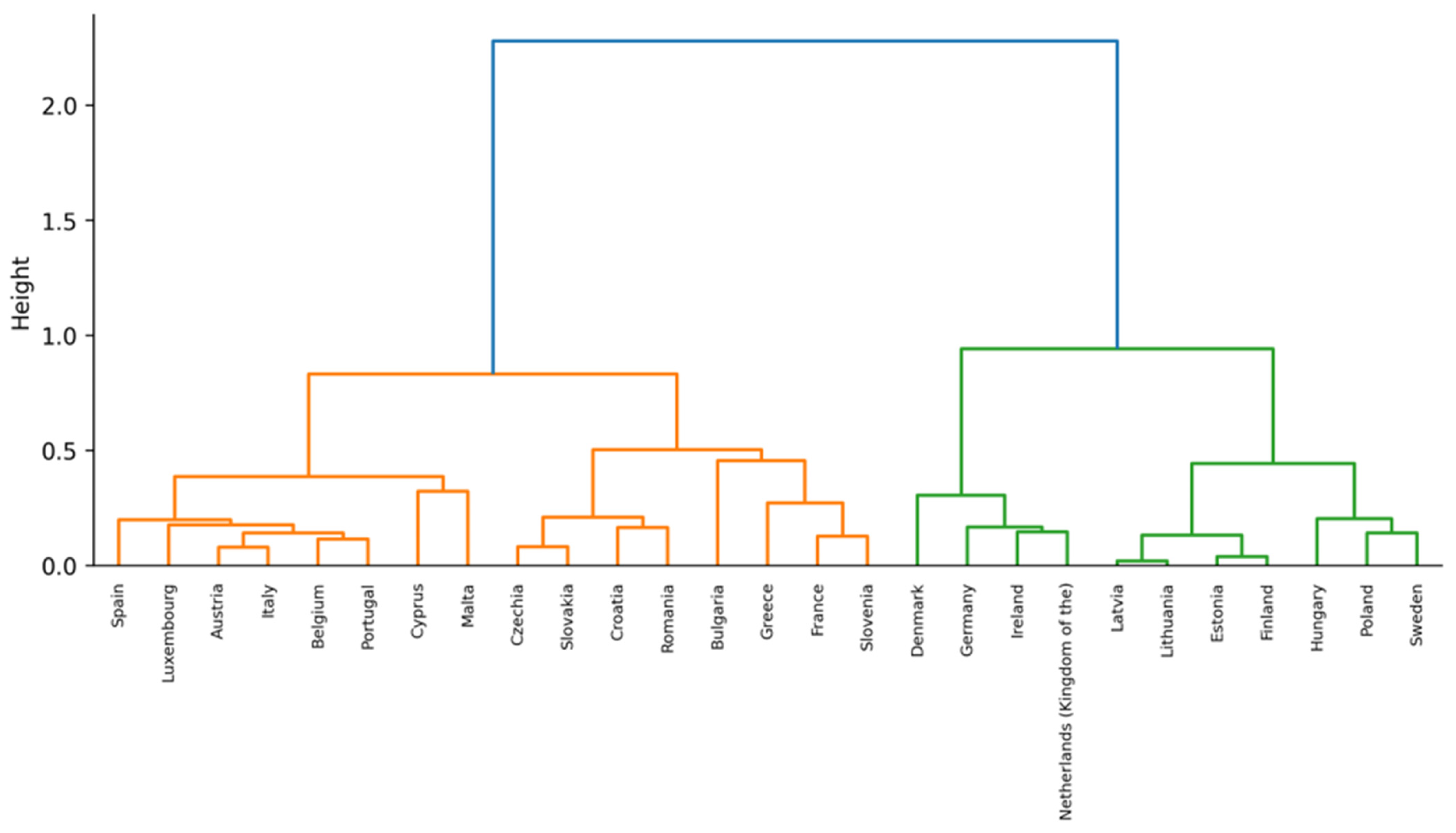
As shown in Table 4 above, Regime 1 contains 16 countries and is dominated by enteric fermentation (46.0%), manure management (16.7%), and synthetic fertilisers (14.1%); Regime 2 contains 11 countries and is dominated by drained organic soils (56.4%) and enteric fermentation (20.7%). Country assignments and the dendrogram are reported in Table A2 and Figure A1.
Ward and PAM agree for 26 of 27 countries, with Denmark the only mismatch (ARI = 0.852; see Table A2). Temporal partitions are identical in 2002–2005, 2006–2009, and 2010–2013 (ARI = 1.000), shift markedly in 2014–2017 (ARI = 0.287), and realign toward the recent structure thereafter (see Table A3; Figure S3).
Bootstrap co-clustering is high within the two Primary9 regimes (mean probability 0.949) and low between them (0.037), indicating recent-period classification stability under the Primary9 definition. This should not be read as a composition-invariant taxonomy: the Primary9–CoDA6 ARI is −0.003, and leave-one-source-out analysis shows that drained organic soils are a defining dimension of the partition (see Table A5 and Table A6; Tables S12–S14). The lower 2021–2023 ARI relative to 2018–2020 arises from a single borderline reassignment (Bulgaria) under the fixed k = 2 Ward partition, illustrating that greater temporal overlap with 2020–2023 does not guarantee a larger ARI in an unsupervised classification. Turning from regime stability to inter-bloc convergence, Table 5 below summarises the emission-weighted Hellinger, equal-country Hellinger, and CoDA6 Aitchison trends over 2002–2023.
Table 5.
Trends in EU-27–Mercosur-4 structural distance, 2002–2023.
As shown in Table 5 above, the emission-weighted Hellinger distance was essentially unchanged from 2002 to 2023 (0.4486 to 0.4494; +0.18%), with no statistically supported directional trend (tau = −0.1775, p = 0.248). The lag-1 autocorrelation was −0.142, and the Hamed–Rao robustness test remained non-significant (see Table S17). Thus, aggregate emission-weighted bloc structures do not show statistically supported convergence.
The equal-country Hellinger distance declined by 4.5% (0.4415 to 0.4214; tau = −0.6883, p < 0.001), indicating convergence in the arithmetic-mean national source profile. Its lag-1 autocorrelation was 0.794, and Hamed–Rao inference remained significant (see Table S17). CoDA6 Aitchison distance also declined by 5.2% (2.900 to 2.748; tau = −0.6104, p < 0.001; lag-1 autocorrelation = 0.739), but CoDA6 refers only to the reclosed, strictly positive six-part subcomposition. It therefore provides separate log-ratio evidence rather than confirmation of Primary9/Hellinger convergence. The contrast between the emission-weighted and equal-country Hellinger trajectories is shown in Figure 4, below.
Figure 4.
Pre-application structural distance between EU-27 and Mercosur-4 agricultural GHG profiles, 2002–2023. The solid line represents the emission-weighted Hellinger distance, while the dashed line represents the equal-country Hellinger distance. Lower values indicate greater similarity in source composition. Data source: FAOSTAT emissions totals (GT). The author created this figure using R 4.6.1 in RStudio 2026.07.0.
Figure 4 illustrates the contrasting evolution of the two EU-27–Mercosur-4 Hellinger-distance estimands over 2002–2023. The emission-weighted distance remains broadly stable, moving from 0.4486 in 2002 to 0.4494 in 2023, with no statistically supported directional trend (tau = −0.1775, p = 0.248). This indicates that the aggregate bloc-level source compositions, which give greater influence to larger national emitters, did not exhibit significant structural convergence over the study period.
In contrast, the equal-country Hellinger distance declines from 0.4415 to 0.4214, a reduction of 4.5%, with a statistically significant negative trend (tau = −0.6883, p < 0.001). This result indicates convergence in the average national source profile when each country receives equal weight. The divergence between the two trajectories confirms that convergence is estimand-specific; representative national compositions became more similar across the two blocs, while the aggregate emission-weighted structures remained comparatively stable. As all observations precede the provisional application of the EU–Mercosur Interim Trade Agreement in 2026, the figure should be interpreted as a pre-application structural baseline rather than as evidence of trade-policy effects.
Annual Hellinger distances are reported in Table S6, the complete CoDA6 annual series in Table S11, and the mean of all 108 annual cross-bloc country-pair distances in Table S20. The latter declined from 0.4815 in 2002 to 0.4629 in 2023 (−3.9%; tau = −0.6537, p < 0.001; Theil–Sen slope = −0.0010 per year), showing that average EU–Mercosur country-to-country separation decreased even though the aggregate emission-weighted bloc distance did not. This pairwise robustness estimand is conceptually distinct from both the emission-weighted bloc distance and the distance between equal-country arithmetic-mean bloc profiles. While these results concern between-bloc separation, within-bloc structural dispersion provides a complementary perspective on whether national source profiles are becoming more or less heterogeneous over time. Table 6 below reports this analysis for both blocs.
Table 6.
Within-bloc structural dispersion and sigma-convergence, 2002–2023.
As shown in Table 6 above, EU within-bloc Hellinger dispersion increases by 6.4% (0.3314 to 0.3526; tau = 0.9048, p < 0.001), indicating compositional sigma-divergence among the fixed EU-27 cohort. Mercosur-4 dispersion declines by 17.6% but without statistical support (tau = −0.2294, p = 0.135), and the small four-country sample makes this series sensitive to individual members. CoDA6 gives the same direction for the EU but a statistically supported decline within Mercosur-4 (see Tables S15 and S17). Hence, within-Mercosur convergence is metric- and boundary-dependent rather than a general result. To determine whether the two blocs are nevertheless separated in recent multivariate compositional space, Table 7 reports PERMANOVA jointly with PERMDISP diagnostics for the 2020–2023 country-mean profiles.
Table 7.
PERMANOVA and PERMDISP tests of EU-27–Mercosur-4 structural separation, 2020–2023.
As shown in Table 7 above, for recent 2020–2023 Primary9 profiles, PERMANOVA is significant (pseudo-F = 7.398, R2 = 0.2033, p = 0.004), but PERMDISP is also significant (p = 0.021). The Primary9 result therefore requires qualification because significant dispersion heterogeneity prevents interpreting PERMANOVA as evidence of a pure compositional-location difference. CoDA6 yields clearer evidence of location separation (pseudo-F = 19.406, R2 = 0.4009, p < 0.001) with non-significant PERMDISP (p = 0.266), but this refers to the separate six-part subcomposition. The 27-versus-4 sample imbalance further limits precision for Mercosur. Directionally, the larger EU-27 group is also the more dispersed group in the same recent Primary9 Hellinger space; the mean pairwise distance among 2020–2023 country-mean profiles is 0.352 for EU-27 and 0.144 for Mercosur-4. This is the conservative, rather than liberal, configuration described by Anderson and Walsh [50]. The significant Primary9 PERMANOVA result (p = 0.004) is therefore not readily explained by the liberal small-group/high-dispersion configuration; however, the significant PERMDISP result still prevents a pure location-only interpretation.
Table 8 decomposes the squared-Hellinger distance by emission source for the early and recent four-year periods.
Table 8.
Source contributions to the EU-27–Mercosur-4 Hellinger distance.
As shown in Table 8 above, the recent emission-weighted squared-Hellinger decomposition is concentrated in drained organic soils (55.2%), enteric fermentation (14.0%), manure left on pasture (12.8%), and manure management (10.8%), jointly accounting for 92.8% of structural distance. These percentages quantify contributions to compositional separation, not absolute emission magnitude, mitigation potential, or causal importance. Country-specific drained-organic-soil shares are reported in Table S21; in 2020–2023, they range from 0% in Paraguay to 4.13% in Argentina within Mercosur-4, while several northern/eastern EU countries have much larger shares. This heterogeneity helps explain why drained organic soils strongly affect both the weighted distance decomposition and EU clustering.
The size of the drained-organic-soils contribution also depends on Hellinger geometry. In the recent emission-weighted Primary9 profiles, this source represents 31.59% of EU emissions but only 0.86% of Mercosur emissions (a gap of 30.73 percentage points). The squared-Hellinger contribution is 55.24%, whereas the same source accounts for 31.62% of the sum of absolute inter-bloc share gaps; enteric fermentation accounts for 33.99% under that latter allocation. The near-zero Mercosur share therefore helps explain the elevated 55.24% squared-Hellinger contribution, without negating the substantial underlying difference in raw shares (see Table A7).
The CoDA6 variation matrix summarises relative log-ratio variability among the six strictly positive sources (see Table S16). Because drained organic soils are excluded from CoDA6, these diagnostics describe a different subcomposition from the Primary9 decomposition and are not used to validate the 55.2% Primary9 contribution.
4.1. Influence and Source-Omission Robustness
Country influence differs by estimand. In Mercosur-4 leave-one-out tests, the equal-country Hellinger trend remains negative and significant after every omission, whereas the weighted trend is generally non-significant and becomes significant only when Brazil is excluded (see Table A4). This is consistent with Brazil’s 73.7% share of recent Mercosur Common9 emissions. Across 27 EU leave-one-out specifications, the equal-country Theil–Sen slope remains negative and significant, while only 7.4% of weighted specifications are significant (see Table S18). These diagnostics reinforce the limited power of a four-country Mercosur comparison and the sensitivity of emission-weighted inference to dominant emitters.
Source-omission tests show the strong boundary dependence of the weighted result (see Table S19). Most importantly, after excluding drained organic soils, the weighted eight-part Hellinger distance declines from 0.3403 in 2002 to 0.2999 in 2023 (−11.88%), with a statistically supported declining trend (tau = −0.7229, p < 0.001), whereas Primary9 itself has no supported weighted trend. Thus, convergence without drained organic soils is a different eight-part result and does not overturn the Primary9 finding. Omitting synthetic fertilisers reverses the weighted trend to a significant increase (+3.96%; tau = 0.6623, p < 0.001), showing that the direction of the aggregate weighted slope depends on the balance among source-share gaps. This is a compositional sensitivity result rather than evidence that synthetic fertiliser emissions causally determine convergence.
Other boundary checks are also interpreted narrowly. Adding on-farm energy use to the EU profile preserves strong but imperfect agreement with Primary9 (ARI = 0.852; see Table S9). Rice cannot be added to the harmonised inter-bloc panel without imputation, because EU rice coverage is only 176/594 observations, whereas Mercosur is complete. The Mercosur10 analysis therefore assesses within-Mercosur sensitivity only and is not an inter-bloc rice robustness test (see Tables S5 and S10).
The new Rice10-Z inter-bloc check (see Table A7) gives an emission-weighted Hellinger distance of 0.4461 in 2002 and 0.4476 in 2023 (+0.32%; Kendall τ = −0.1342, p = 0.382), compared with 0.4486 and 0.4494 (+0.18%; τ = −0.1775, p = 0.248) for Primary9. The equal-country Rice10-Z distance declines from 0.4406 to 0.4205 (−4.56%; τ = −0.7056, p < 0.001), compared with 0.4415 to 0.4214 (−4.54%; τ = −0.6883, p < 0.001) for Primary9. Hence, the distinction between emission-weighted and equal-country trends persists under conditional rice inclusion, but this calculation cannot establish the missing rice entries as true zeros.
4.2. Assessment of the Hypotheses
H1 is supported with qualification for the 2020–2023 profiles: Primary9 PERMANOVA is significant, but significant PERMDISP prevents attributing the result solely to compositional-location separation; CoDA6 provides clearer location separation for its distinct six-part subcomposition (see Table 7). H2 receives estimand-specific support. The emission-weighted Primary9 Hellinger distance does not show statistically supported convergence, whereas the equal-country Primary9 Hellinger distance declines significantly. CoDA6 Aitchison distance also declines, but only for the reclosed six-part strictly positive subcomposition (see Table 5; Tables S17 and S20).
H3 is supported with qualification under the Primary9 definition: a relatively stable two-regime EU structure is identified, but the classification is strongly dependent on drained organic soils and is not composition-invariant (see Table 4; Table A5 and Table A6). H4 is not supported because EU mean pairwise Hellinger dispersion rises by 6.41%, indicating sigma-divergence; CoDA6 shows the same directional conclusion (see Table 6 and Table S15). E1 is descriptive rather than confirmatory; the decomposition finds that four sources account for 92.8% of the recent emission-weighted squared-Hellinger distance, but no ex ante threshold was specified for the number or share of sources required.
5. Discussion
The principal finding is estimand-specific rather than suggestive of general convergence. Agricultural GHG scale diverged between the blocs; Common9 emissions fell by 10.0% in the fixed EU-27 cohort but rose by 26.1% in Mercosur-4. At the same time, the equal-country Primary9 distance declined, while the aggregate emission-weighted Primary9 distance did not. The average of all cross-bloc country-pair distances also declined. These results show increasing similarity in the arithmetic-mean national profiles and in paired country-level source structures without statistically supported convergence of the aggregate-weighted bloc profiles. This distinction is consistent with the broader convergence literature, where results depend on whether emissions are analysed in levels, per-capita terms, intensities, or distributions [19,20]; source-composition convergence is a separate concept.
Recent EU–Mercosur separation is likewise boundary- and dispersion-sensitive. Primary9 PERMANOVA is significant, but significant PERMDISP precludes interpreting it as a pure centroid difference. CoDA6 provides clearer location separation, yet CoDA6 excludes the zero-containing sources and therefore estimates a different log-ratio subcomposition. Mercosur’s aggregate profile is also highly concentrated in Brazil, which accounts for 73.7% of recent Common9 emissions, while the statistical comparison contains only four Mercosur countries. Accordingly, the weighted bloc profile is substantively meaningful as an aggregate emissions composition but should not be read as a typical Mercosur country.
The EU clustering result should also be interpreted within its compositional boundary. Primary9 identifies a relatively stable two-regime partition in 2020–2023, with high within-cluster bootstrap co-membership, but omission of drained organic soils or restriction to CoDA6 substantially changes the classification. This result therefore describes regimes under the Primary9 definition rather than a universal taxonomy of EU agriculture. This is compatible with increasing EU pairwise dispersion; a stable two-group partition can coexist with greater distances among individual country profiles.
Drained organic soils are central to that boundary dependence. They contribute 55.2% of the recent emission-weighted squared-Hellinger distance and strongly affect the Primary9 clustering partition. This identifies a structural monitoring priority, not a direct estimate of mitigation effectiveness. A review of the literature shows why the category matters; drained agricultural organic soils can be large sources of GHGs and are commonly treated within AFOLU/LULUCF accounting [24]. Rewetting can materially reduce CO2 emissions from drained agricultural peat soils, although methane responses and site conditions require case-specific assessment [51]. Those mitigation statements come from external evidence, not from the present distance decomposition.
This source ranking is a property of the selected metric, not a geometry-invariant measure of importance. Under the alternative absolute-share-gap allocation, drained organic soils contribute 31.62% rather than 55.24% to recent weighted inter-bloc separation, and enteric fermentation (33.99%) becomes the largest contributor. When conditional rice inclusion is applied, the drained-organic-soils squared-Hellinger contribution remains 55.14% and its absolute-gap allocation is 31.50%. These results distinguish a real source-share contrast from amplification associated with the square-root representation.
The same distinction applies to livestock sources. Enteric fermentation, manure left on pasture and manure management contribute materially to the EU–Mercosur structural gap, but their decomposition shares do not rank mitigation cost-effectiveness. The external literature supports attention to livestock management because enteric methane is important in Brazil [5], Paraguay [6], and Uruguay [7], while the appropriate intervention depends on production system, feed, pasture, manure management, and national conditions. The present analysis therefore identifies where structures differ; it does not estimate the causal effectiveness of feed, pasture, manure, carbon-credit, or other mitigation instruments.
The pre-application design is central. The observation data ended in 2023; this study therefore establishes a structural baseline rather than an effect of the EU–Mercosur agreements. Prospective studies indicate that trade liberalisation may affect deforestation and land-use change [12,13], but these channels are outside Primary9. The exclusion is deliberate; adding deforestation would change the analytical boundary from the harmonised agriculture-related source bundle toward broader AFOLU. Post-application evaluation should therefore examine agricultural source composition and land-use change with separate indicators rather than infer one from the other.
The study’s contribution is consequently diagnostic. It provides three complementary views of inter-bloc structure—aggregate emission-weighted profiles, equal-country arithmetic-mean profiles, and mean cross-bloc country-pair distances—plus a separate CoDA6 log-ratio robustness analysis. Their differences are substantive rather than contradictory. Monitoring after 2026 should retain these distinctions and should report absolute source emissions alongside compositional shares, because closure means that a share can rise when another source falls, even if the source’s own emissions are unchanged.
Limitations and Scope Conditions
The present results are subject to several limitations. FAOSTAT Tier 1 estimates are harmonised national estimates rather than direct farm measurements. Published external validation has compared FAOSTAT drained-organic-soil estimates with official UNFCCC country inventories and found substantial cross-country agreement [25]; the present study does not independently reconstruct and reconcile each of the 31 national inventory series, so that country-specific differences in methods, updates, uncertainty, and sector allocation remain a limitation. Meanwhile, drained organic soils and savanna fires may be classified differently across national inventory frameworks. Furthermore, Primary9 adopts a selected common-source boundary that excludes rice cultivation from the confirmatory inter-bloc comparison, while Rice10-Z evaluates its conditional inclusion as a sensitivity analysis. On-farm energy use, forest land, deforestation, and broader land-use change remain outside the harmonised Primary9 boundary. Moreover, compositional closure means share changes must be interpreted alongside absolute emissions. The present conclusions depend partly on metric and boundary choice, as shown by Hellinger/Primary9 versus Aitchison/CoDA6 and source-omission results. Also, Mercosur includes only four countries and Brazil dominates the emission-weighted totals, limiting power and influencing balance. Meanwhile, national averages mask regional and production-system heterogeneity. Potentially relevant soil-pressure indicators cannot necessarily be integrated into an annual 2002–2023 panel; for example, Eurostat/JRC’s severe soil-erosion-by-water indicator (sdg_15_50) provides only four benchmark observations (2000, 2010, 2016 and 2023), with a methodological/resolution difference for 2000 [52]. Interpolating the missing years would create synthetic annual data; so, this indicator was not used in the longitudinal analysis.
A further qualification concerns the new Rice10-Z sensitivity and the interpretation of source decompositions. The 418 previously missing EU rice cells were assigned zero only to test one plausible boundary scenario, not because their zero status had been independently demonstrated for all years. Eurostat’s evidence of eight producing countries in 2022 and 2023 [33,34] does not validate earlier country-year cells. In addition, a source with a very small share in one bloc can receive a comparatively large squared-Hellinger contribution; the absolute-gap comparison in Table A7 is reported to prevent this metric-specific percentage from being interpreted as a geometry-independent ranking.
6. Conclusions and Policy Implications
This study establishes a pre-application benchmark of agricultural GHG emissions scales and source structure in a fixed EU-27 geographical cohort and Mercosur-4 over 2002–2023. Common9 emissions declined by 10.0% in the EU-27 but increased by 26.1% in Mercosur-4. Convergence was partial and estimand-specific; the aggregate emission-weighted Primary9 Hellinger distance showed no statistically supported trend, whereas the equal-country Primary9 distance declined. The CoDA6 Aitchison distance also declined, but only for its separate six-part strictly positive subcomposition.
Equal-country profile similarity therefore increased without convergence of the aggregate weighted bloc structures. The mean cross-bloc country-pair distance also declined, while EU within-bloc dispersion increased. The recent (2020–2023) EU country profiles form a relatively stable two-regime partition under Primary9, but the partition depends strongly on drained organic soils and should not be interpreted as composition-invariant. These distinctions are central to the contribution of this study.
The source decomposition identifies structural contributors, not mitigation rankings. Drained organic soils, enteric fermentation, manure left on pasture, and manure management jointly account for 92.8% of the recent emission-weighted squared-Hellinger distance. The appropriate interpretation indicates these to be priorities for source-resolved monitoring and further country-specific evaluation. Decisions about restoration, rewetting, livestock management, or other interventions require separate evidence regarding absolute emissions, feasibility, effectiveness, costs, and local conditions. The 55.2% figure is specific to squared-Hellinger geometry; under an absolute-share-gap allocation, the corresponding drained-organic-soils share is 31.62%.
The signing of the EU–Mercosur Partnership Agreement (EMPA) and Interim Trade Agreement (iTA) on 17 January 2026 in Asunción, followed by the provisional application of the iTA from 1 May 2026, gives this benchmark immediate relevance for environmental monitoring. Because the empirical data ended in 2023, the present results do not measure effects of the agreement; rather, they provide a reference against which post-application changes can be evaluated. This temporal separation is consistent with the analytical design of this study.
Post-application monitoring should report absolute source emissions together with compositional indicators and should distinguish aggregate emission-weighted from equal-country measures. This would allow future assessments to determine whether changes reflect shifts in the scale of emissions, compositional reallocation, or country-specific developments rather than treating all forms of convergence as equivalent.
Land-use change should be assessed separately. Primary9 does not include deforestation or broader forest conversion, and the analysis therefore cannot capture all environmental channels through which trade or agricultural expansion may operate. Dedicated land-use indicators should complement, not be merged uncritically with, the agricultural source profile. Where soil-condition indicators are used, their temporal coverage must also be respected; the Eurostat/JRC severe water-erosion series, for example, is available only for benchmark years and cannot support an annual 2002–2023 trend without interpolation [52].
These policy implications should be interpreted within the limitations and scope conditions set out in Section Limitations and Scope Conditions, especially the harmonised-data boundary, the small Mercosur-4 sample, compositional-boundary sensitivity, and the non-causal design.
Future research should extend the dataset into the post-2026 period, reconcile harmonised FAOSTAT estimates with country-submitted inventories, incorporate broader land-use outcomes using temporally appropriate datasets, and exploit higher-resolution regional or production-system information. Once sufficient post-application observations accumulate, the present benchmark can support causal or quasi-experimental work. Until then, its appropriate role is structural diagnosis and monitoring rather than attribution of policy effects.
Supplementary Materials
The following supporting information can be downloaded at: https://www.mdpi.com/article/10.3390/gases6040051/s1, Supplementary Tables S1–S21 provide the balanced-window assessment; country- and source-specific trends; source profiles; concentration and diversity measures; Hellinger and Aitchison distances; bloc-specific ten-source robustness; EU cluster validation and sensitivity; within-bloc dispersion; autocorrelation-robust trend inference; leave-one-country/source-out analyses; the annual mean cross-bloc country-pair distance; and country-level recent drained-organic-soil shares. Supplementary Figures S1–S3 report within-bloc structural dispersion, source contributions to structural distance, and temporal persistence of EU Primary9 regimes.
Funding
This research was funded by national funds through FCT—Fundação para a Ciência e a Tecnologia, I.P., under the strategic funding of the University of Coimbra Institute for Legal Research (UCILeR), project UIDB/04643/2020.
Institutional Review Board Statement
Not applicable. This study used aggregate secondary data and did not involve human participants or animals.
Informed Consent Statement
Not applicable. This study did not involve human participants.
Data Availability Statement
Publicly available datasets were analysed in this study. Annual agricultural greenhouse-gas emissions were obtained from the FAOSTAT Emissions Totals (GT) database, using the element “Emissions (CO2eq) (AR5)”. The data are publicly available from the Food and Agriculture Organization of the United Nations (FAO) through FAOSTAT at https://www.fao.org/faostat/en/#data/GT (accessed on 9 October 2026). The processed analytical dataset supporting the findings of this study is available from the corresponding author upon reasonable request.
Acknowledgments
During the preparation of this manuscript, the author used Grammarly (version 1.2.96.1473) solely for language and grammatical editing and ChatGPT (OpenAI, San Francisco, CA, USA, GPT-5.6 Sol; accessed on 6 October 2026) for language and editorial assistance and to assist in the preparation of Figure 1. All quantitative analyses and data-derived visualizations were produced and verified by the author using the analytical procedures and software reported in the manuscript. The author takes full responsibility for the content of this publication.
Conflicts of Interest
The author declares no conflicts of interest.
Abbreviations
The following abbreviations are used in this manuscript:
| AFOLU | Agriculture, forestry, and other land use |
| AI | Artificial intelligence |
| AR5 | Fifth Assessment Report of the Intergovernmental Panel on Climate Change |
| ARI | Adjusted Rand index |
| BH | Benjamini–Hochberg |
| CAP | Common Agricultural Policy |
| CH4 | Methane |
| CO2 | Carbon dioxide |
| CO2eq | Carbon dioxide equivalent |
| CoDA6 | Six-source strictly positive compositional-data subcomposition |
| Common9 | Harmonised common nine-source emission total |
| EMPA | EU–Mercosur Partnership Agreement |
| EU | European Union |
| EU-27 | 27 European Union Member States included in the study |
| EU10 | Ten-source EU robustness specification |
| FAO | Food and Agriculture Organization of the United Nations |
| FAOSTAT | Statistical database of the Food and Agriculture Organization of the United Nations |
| FCT | Fundação para a Ciência e a Tecnologia |
| GHG | Greenhouse gas |
| GT | FAOSTAT Emissions Totals domain |
| HHI | Herfindahl–Hirschman Index |
| INIAV | National Institute for Agricultural and Veterinary Research |
| IPCC | Intergovernmental Panel on Climate Change |
| IQR | Interquartile range |
| iTA | Interim Trade Agreement |
| kt | Kilotonnes |
| Mercosur | Southern Common Market (Mercado Común del Sur) |
| Mercosur-4 | Argentina, Brazil, Paraguay, and Uruguay |
| Mercosur10 | Ten-source Mercosur robustness specification |
| MRV | Measurement, reporting, and verification |
| N2O | Nitrous oxide |
| PAM | Partitioning around medoids |
| PERMANOVA | Permutational multivariate analysis of variance |
| PERMDISP | Permutational analysis of multivariate dispersions |
| Primary9 | Harmonised primary nine-source specification |
| SD | Standard deviation |
| SEEG | Sistema de Estimativas de Emissões e Remoções de Gases de Efeito Estufa |
Appendix A
Table A1.
Variable inclusion/exclusion, coverage, and analytical role.
Table A2.
EU-27 country-level Primary9 regime assignments and profile diagnostics.
Table A3.
Temporal persistence of EU-27 Primary9 structural regimes.
Table A4.
Mercosur-4 leave-one-country-out sensitivity of EU-27–Mercosur-4 Hellinger-distance trends.
Table A5.
Consolidated EU-27 cluster-robustness diagnostics.
Table A6.
Leave-one-source-out stability of the EU-27 Primary9 structural regime classification.
Table A7.
Conditional inter-bloc rice inclusion and squared-Hellinger geometry sensitivity.
Figure A1.
EU-27 Ward.D2 dendrogram for the 2020–2023 Primary9 profiles (k = 2). Notes: The dendrogram provides descriptive support for the Ward hierarchy; the number of regimes is justified by average silhouette and cross-method validation rather than visual inspection alone. The author created this figure using R 4.6.1 in RStudio 2026.07.0.
References
- Nabuurs, G.-J.; Mrabet, R.; Abu Hatab, A.; Bustamante, M.; Clark, H.; Havlik, P.; House, J.; Mbow, C.; Ninan, K.N.; Popp, A.; et al. Agriculture, Forestry and Other Land Uses (Chapter 7). In IPCC 2022: Climate Change 2022: Mitigation of Climate Change. Contribution of Working Group III to the Sixth Assessment Report of the Intergovernmental Panel on Climate Change; Cambridge University Press: Cambridge, UK, 2022; pp. 747–860. [Google Scholar] [CrossRef] [Scilit]
- Dace, E.; Blumberga, D. How do 28 European Union Member States perform in agricultural greenhouse gas emissions? It depends on what we look at: Application of the multi-criteria analysis. Ecol. Indic. 2016, 71, 352–358. [Google Scholar] [CrossRef] [Scilit]
- European Court of Auditors. Common Agricultural Policy and Climate: Half of EU Climate Spending but Farm Emissions Are Not Decreasing; Special Report 16/2021; European Court of Auditors: Luxembourg, 2021. Available online: https://www.eca.europa.eu/en/publications?did=58913 (accessed on 9 October 2026).
- Stetter, C.; Buser, V.; Finger, R. Policy mixes and major emission reductions in European agriculture. Food Policy 2026, 140, 103084. [Google Scholar] [CrossRef] [Scilit]
- Bieluczyk, W.; Cherubin, M.R.; Cerri, C.E.P.; Siqueira-Neto, M.; Abdalla-Filho, A.L.; Castro, J.I.A.; Locatelli, J.L.; Tsai, S.M.; Camargo, P.B. Greenhouse gas fluxes in Brazilian climate-smart agricultural and livestock systems: A systematic and critical overview. J. Clean. Prod. 2024, 464, 142782. [Google Scholar] [CrossRef] [Scilit]
- Ministerio del Ambiente y Desarrollo Sostenible (MADES), Paraguay. Resumen del Capítulo 2, Inventario Nacional de Gases de Efecto Invernadero, Serie 1990–2017, Tercer Informe Bienal de Actualización (IBA3). 2021. Available online: https://www.mades.gov.py/wp-content/uploads/2025/04/Resumen_del_capitulo_del_INGEI_del_Tercer_Informe_Bienal_de_Actualizacion_del_Paraguay_%E2%80%93_IBA3-compri.pdf (accessed on 9 October 2026).
- Ministerio de Ambiente, Uruguay. Inventarios Nacionales de Gases de Efecto Invernadero (INGEI), Including Serie 1990–2022. 2024. Available online: https://www.gub.uy/ministerio-ambiente/politicas-y-gestion/inventarios-nacionales-gases-efecto-invernadero-ingei (accessed on 9 October 2026).
- Subsecretaría de Ambiente de la República Argentina. Primer Informe Bienal de Transparencia (IBT1) and Informe Nacional de Inventario (INI), Inventory Series 1990–2022. 2024. Available online: https://www.argentina.gob.ar/noticias/argentina-presento-su-primer-informe-bienal-de-transparencia (accessed on 9 October 2026).
- Palmieri, R.; Amice, C.; Amato, M.; Verneau, F. Beyond the finish line: Sustainability hurdles in the EU-Mercosur Free Trade Agreement. Soc. Sci. 2024, 13, 362. [Google Scholar] [CrossRef] [Scilit]
- Gosselin, L.; Durel, L.; Morin, J.-F. Persistent instability in policy debates: The three-body problem of trade, agriculture and the environment. J. Common Mark. Stud. 2026, 64, 1715–1750. [Google Scholar] [CrossRef] [Scilit]
- European Commission. EU-Mercosur Interim Trade Agreement Starts to Provisionally Apply. Directorate-General for Trade and Economic Security. 30 April 2026. Available online: https://policy.trade.ec.europa.eu/news/eu-mercosur-interim-trade-agreement-starts-provisionally-apply-2026-04-30_en (accessed on 9 October 2026).
- Arima, E.; Barreto, P.; Taheripour, F.; Aguiar, A. Dynamic Amazonia: The EU-Mercosur Trade Agreement and deforestation. Land 2021, 10, 1243. [Google Scholar] [CrossRef] [Scilit]
- Mercado Cordova, J.A.; Koo, Y. Trade-induced land-use transitions and greenhouse gas emissions: The case of the EU-Mercosur free-trade agreement. J. Clean. Prod. 2023, 429, 139327. [Google Scholar] [CrossRef] [Scilit]
- Cesar de Oliveira, S.E.M.; Visentin, J.C.; Pavani, B.F.; Branco, P.D.; de Maria, M.; Loyola, R. The European Union-Mercosur Free Trade Agreement as a tool for environmentally sustainable land use governance. Environ. Sci. Policy 2024, 161, 103875. [Google Scholar] [CrossRef] [Scilit]
- Hagemejer, J.; Stoll, P.-T.; Rudloff, B.; Mensah, K. An Update on the Economic, Sustainability and Regulatory Effects of the Trade Part of the EU-Mercosur Partnership Agreement; European Parliament, Directorate-General for External Policies of the Union: Brussels, Belgium, 2025. [Google Scholar] [CrossRef]
- Harrison, J.; Paulini, S. Reinventing trade, environment and development interlinkages: Lessons from the EU-Mercosur Association Agreement. J. Int. Econ. Law 2024, 27, 723–740. [Google Scholar] [CrossRef]
- Olech, I.; Krupska, K.; Kosior, K. The problem of enforcing environmental clauses in the EU-Mercosur Partnership Agreement in the context of the discrepancy in deforestation indices. Forests 2025, 16, 1821. [Google Scholar] [CrossRef] [Scilit]
- Del Pupo, E. Politicisation and agricultural (post-)exceptionalism in EU-Mercosur Association Agreement negotiations. J. Common Mark. Stud. 2026, 64, 980–1000. [Google Scholar] [CrossRef] [Scilit]
- Strazicich, M.C.; List, J.A. Are CO2 emission levels converging among industrial countries? Environ. Resour. Econ. 2003, 24, 263–271. [Google Scholar] [CrossRef] [Scilit]
- Aldy, J.E. Per capita carbon dioxide emissions: Convergence or divergence? Environ. Resour. Econ. 2006, 33, 533–555. [Google Scholar] [CrossRef] [Scilit]
- Aitchison, J. The statistical analysis of compositional data. J. R. Stat. Soc. Ser. B 1982, 44, 139–160. [Google Scholar] [CrossRef] [Scilit]
- Pawlowsky-Glahn, V.; Egozcue, J.J.; Tolosana-Delgado, R. Modelling and Analysis of Compositional Data; Wiley: Chichester, UK, 2015. [Google Scholar] [CrossRef] [Scilit]
- FAO. FAOSTAT Domain Emissions Totals: Methodological Note, Release October 2023; Food and Agriculture Organization of the United Nations: Rome, Italy, 2023; Available online: https://files-faostat.fao.org/production/GT/GT_en.pdf (accessed on 18 October 2026).
- Tiemeyer, B.; Freibauer, A.; Albiac Borraz, E.; Augustin, J.; Bechtold, M.; Beetz, S.; Beyer, C.; Ebli, M.; Eickenscheidt, T.; Fiedler, S.; et al. A new methodology for organic soils in national greenhouse gas inventories: Data synthesis, derivation and application. Ecol. Indic. 2020, 109, 105838. [Google Scholar] [CrossRef] [Scilit]
- Conchedda, G.; Tubiello, F.N. Drainage of organic soils and GHG emissions: Validation with country data. Earth Syst. Sci. Data 2020, 12, 3113–3137. [Google Scholar] [CrossRef] [Scilit]
- Mohammed, S.; Raihan, A.; Arshad, S.; Ata, B.; Ocwa, A.; Al-Dalahmeh, M.; Harsanyi, E. European Union agro-climate policies toward sustainability: Analyzing emission trends and land use dynamics (1990–2021). Resour. Environ. Sustain. 2025, 21, 100239. [Google Scholar] [CrossRef] [Scilit]
- Verschuuren, J. Achieving agricultural greenhouse gas emission reductions in the EU post-2030: What options do we have? Rev. Eur. Comp. Int. Environ. Law 2022, 31, 246–257. [Google Scholar] [CrossRef] [Scilit]
- Mroczek, R.; Szymańska, E.J.; Tłuczak, A.; Drożdż, J. Determinants of beef trade between the EU and South America and the implications of the EU-Mercosur Agreement for the European beef sector. Sustainability 2026, 18, 2172. [Google Scholar] [CrossRef] [Scilit]
- Koengkan, M. The decline of environmental degradation by renewable energy consumption in the MERCOSUR countries: An approach with ARDL modeling. Environ. Syst. Decis. 2018, 38, 415–425. [Google Scholar] [CrossRef] [Scilit]
- Koengkan, M.; Fuinhas, J.A.; Santiago, R. The relationship between CO2 emissions, renewable and non-renewable energy consumption, economic growth, and urbanisation in the Southern Common Market. J. Environ. Econ. Policy 2020, 9, 383–401. [Google Scholar] [CrossRef] [Scilit]
- Karimi Alavijeh, N.; Salehnia, N.; Salehnia, N.; Koengkan, M. The effects of agricultural development on CO2 emissions: Empirical evidence from the most populous developing countries. Environ. Dev. Sustain. 2023, 25, 12011–12031. [Google Scholar] [CrossRef] [Scilit]
- MERCOSUR. Countries; MERCOSUR: Montevideo, Uruguay, 2026; Available online: https://www.mercosur.int/en/about-mercosur/countries (accessed on 9 October 2026).
- Eurostat. Regions in Europe—2024 Edition: Rice Production in 2022; European Commission: Luxembourg, 2024; Available online: https://ec.europa.eu/eurostat/web/interactive-publications/regions-2024 (accessed on 9 October 2026).
- Eurostat. Regions in Europe—2025 Edition: Rice Production in 2023; European Commission: Luxembourg, 2025; Available online: https://ec.europa.eu/eurostat/web/interactive-publications/regions-2025 (accessed on 9 October 2026).
- Hirschman, A.O. National Power and the Structure of Foreign Trade; University of California Press: Oakland, CA, USA, 1945. [Google Scholar]
- Herfindahl, O.C. Concentration in the U.S. Steel Industry. Doctoral Dissertation, Columbia University, New York, NY, USA, 1950. [Google Scholar]
- Shannon, C.E. A mathematical theory of communication. Bell Syst. Tech. J. 1948, 27, 379–423. [Google Scholar] [CrossRef] [Scilit]
- Legendre, P.; Gallagher, E.D. Ecologically meaningful transformations for ordination of species data. Oecologia 2001, 129, 271–280. [Google Scholar] [CrossRef] [Scilit] [PubMed]
- Mann, H.B. Nonparametric tests against trend. Econometrica 1945, 13, 245–259. [Google Scholar] [CrossRef] [Scilit]
- Kendall, M.G. Rank Correlation Methods, 4th ed.; Charles Griffin: Oklahoma City, OK, USA, 1975. [Google Scholar]
- Sen, P.K. Estimates of the regression coefficient based on Kendall’s tau. J. Am. Stat. Assoc. 1968, 63, 1379–1389. [Google Scholar] [CrossRef]
- Benjamini, Y.; Hochberg, Y. Controlling the false discovery rate: A practical and powerful approach to multiple testing. J. R. Stat. Soc. Ser. B 1995, 57, 289–300. [Google Scholar] [CrossRef] [Scilit]
- Hamed, K.H.; Rao, A.R. A modified Mann–Kendall trend test for autocorrelated data. J. Hydrol. 1998, 204, 182–196. [Google Scholar] [CrossRef] [Scilit]
- Ward, J.H., Jr. Hierarchical grouping to optimize an objective function. J. Am. Stat. Assoc. 1963, 58, 236–244. [Google Scholar] [CrossRef]
- Rousseeuw, P.J. Silhouettes: A graphical aid to the interpretation and validation of cluster analysis. J. Comput. Appl. Math. 1987, 20, 53–65. [Google Scholar] [CrossRef] [Scilit]
- Kaufman, L.; Rousseeuw, P.J. Finding Groups in Data: An Introduction to Cluster Analysis; Wiley: Hoboken, NJ, USA, 1990. [Google Scholar] [CrossRef] [Scilit]
- Hubert, L.; Arabie, P. Comparing partitions. J. Classif. 1985, 2, 193–218. [Google Scholar] [CrossRef] [Scilit]
- Anderson, M.J. A new method for non-parametric multivariate analysis of variance. Austral Ecol. 2001, 26, 32–46. [Google Scholar] [CrossRef] [Scilit]
- Anderson, M.J. Distance-based tests for homogeneity of multivariate dispersions. Biometrics 2006, 62, 245–253. [Google Scholar] [CrossRef] [Scilit] [PubMed]
- Anderson, M.J.; Walsh, D.C.I. PERMANOVA, ANOSIM, and the Mantel test in the face of heterogeneous dispersions: What null hypothesis are you testing? Ecol. Monogr. 2013, 83, 557–574. [Google Scholar] [CrossRef] [Scilit]
- Bianchi, A.; Larmola, T.; Kekkonen, H.; Saarnio, S.; Lång, K. Review of greenhouse gas emissions from rewetted agricultural soils. Wetlands 2021, 41, 108. [Google Scholar] [CrossRef] [Scilit]
- Eurostat; European Commission Joint Research Centre. Area at Risk of Severe Soil Erosion by Water (sdg_15_50), Metadata and Dataset, DOI: 10.2908/sdg_15_50; 2026. Data Points: 2000, 2010, 2016 and 2023. Available online: https://ec.europa.eu/eurostat/databrowser/product/view/sdg_15_50 (accessed on 9 October 2026).
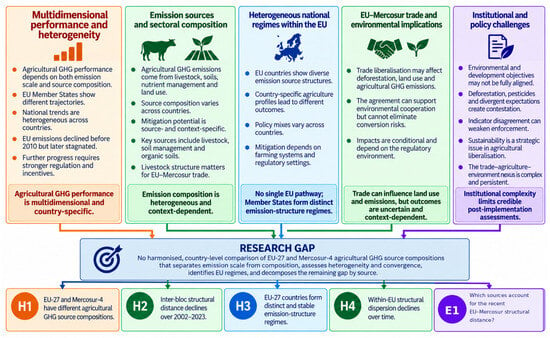
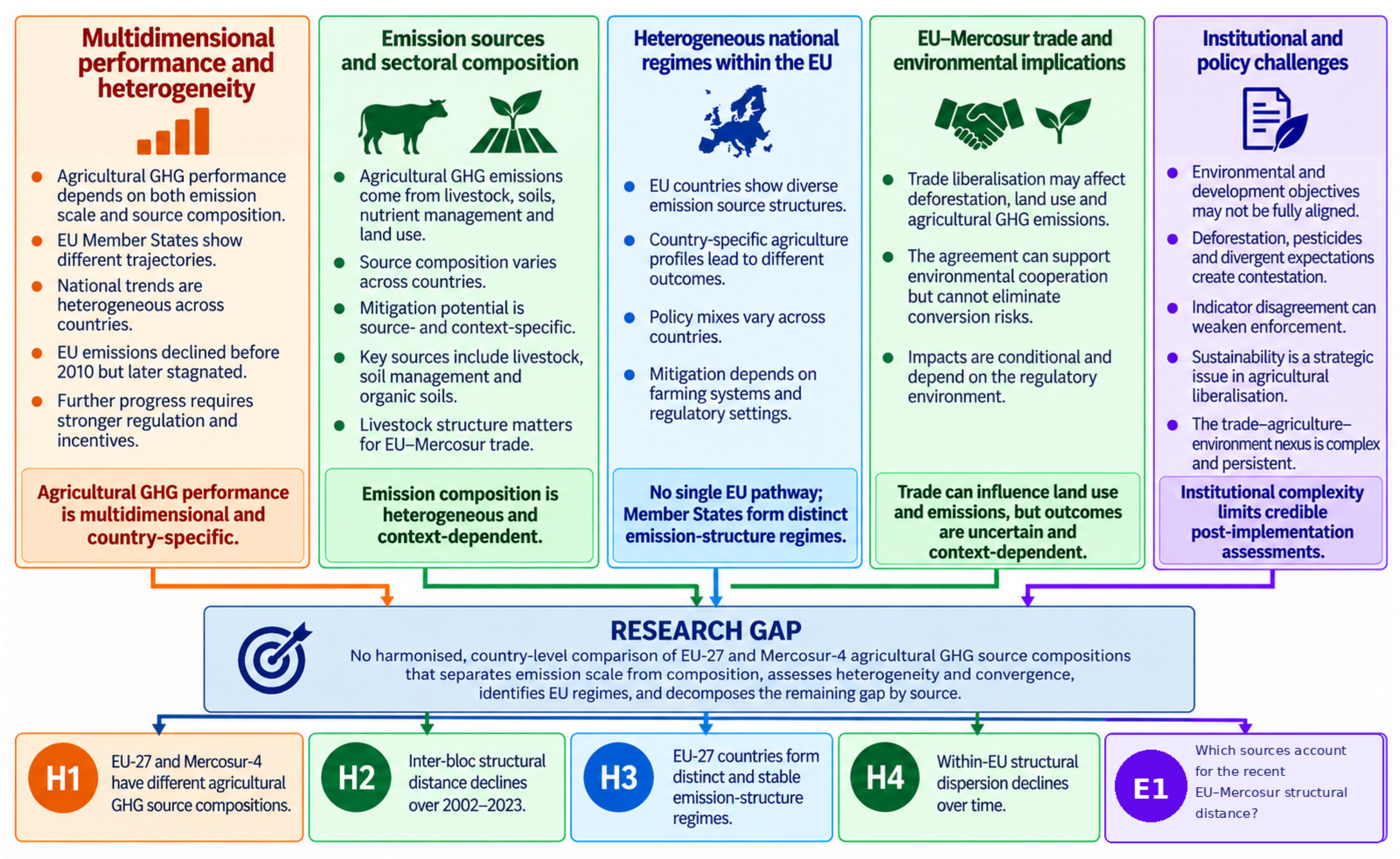
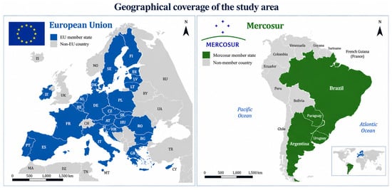
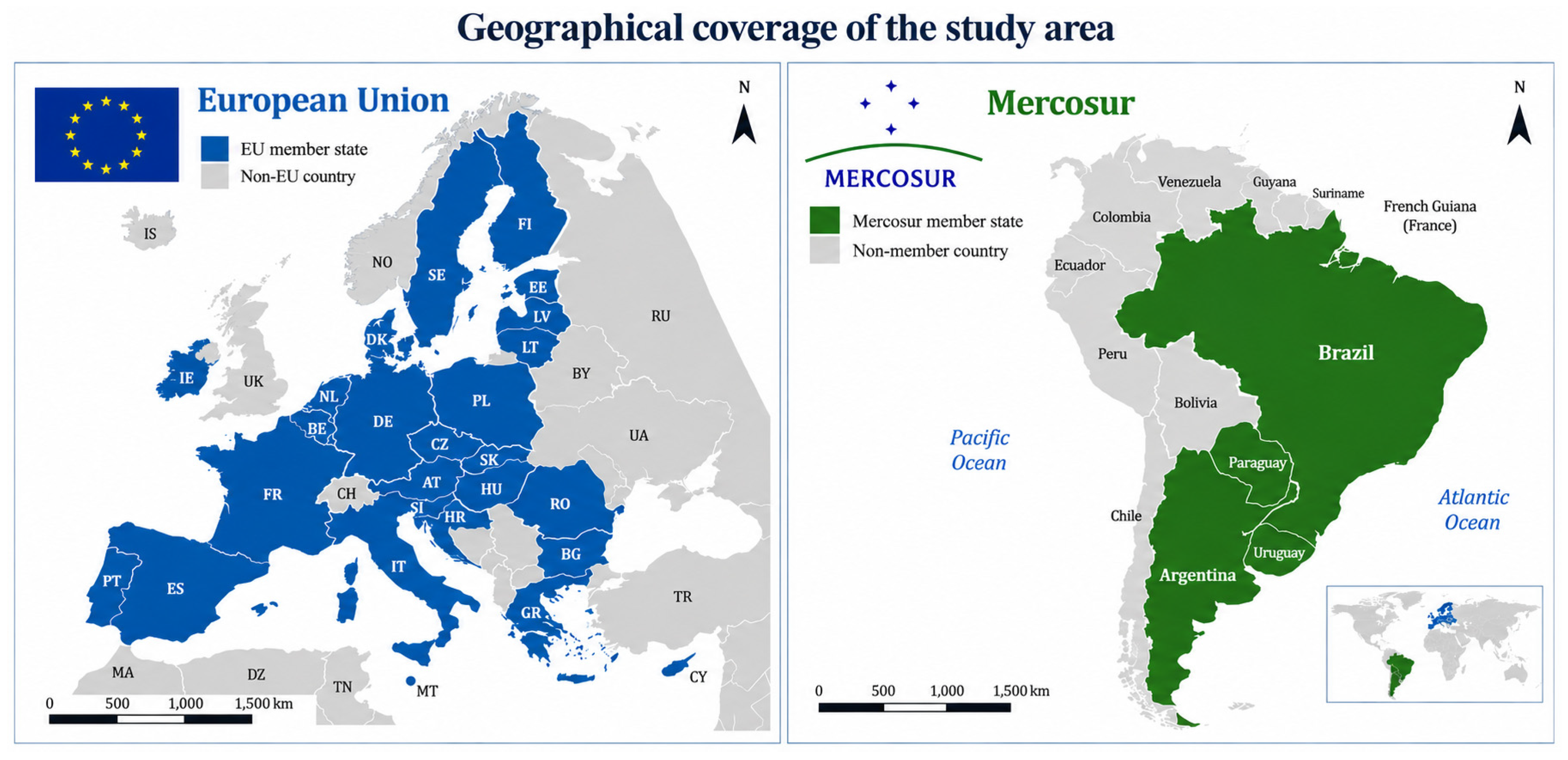
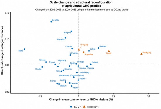
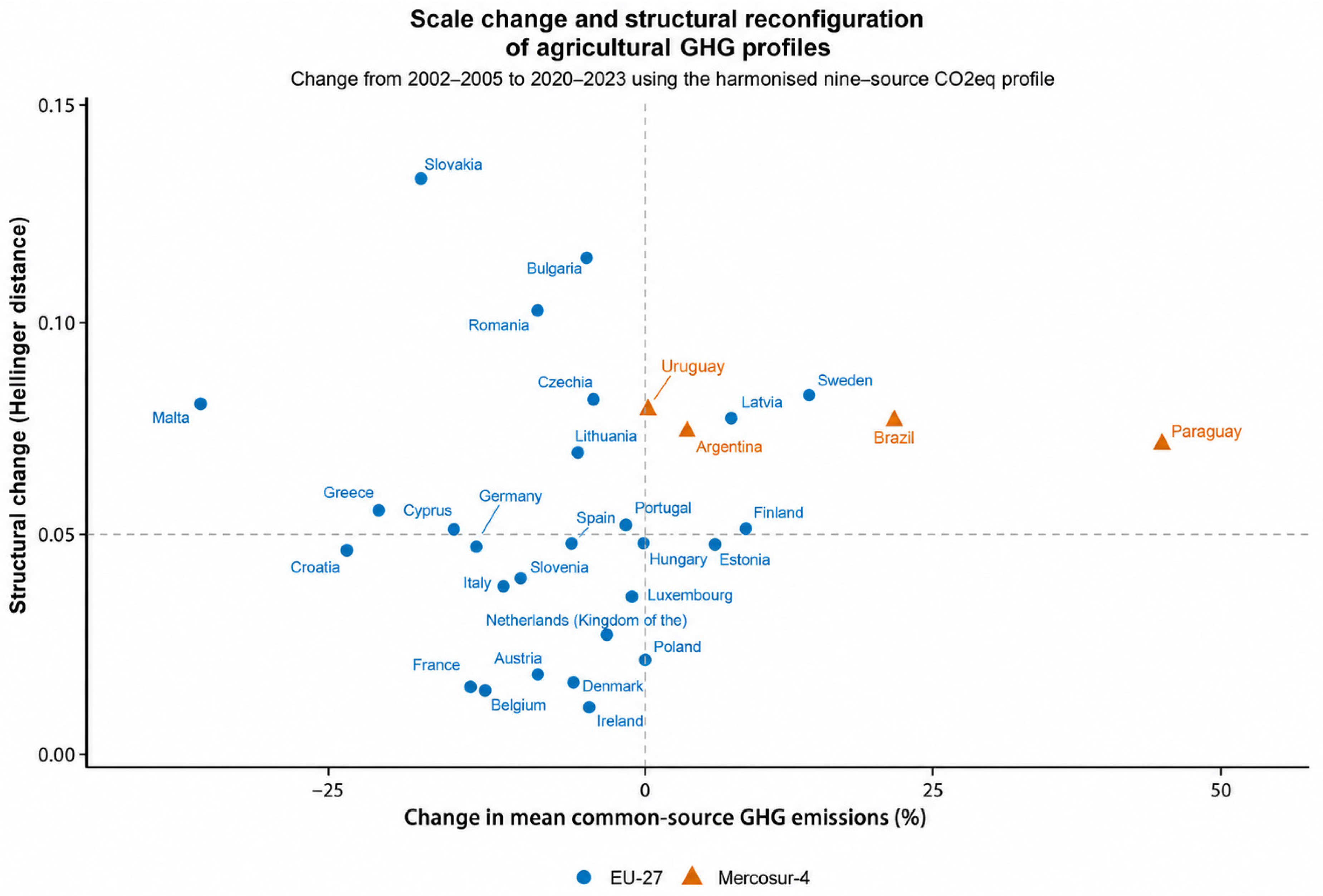
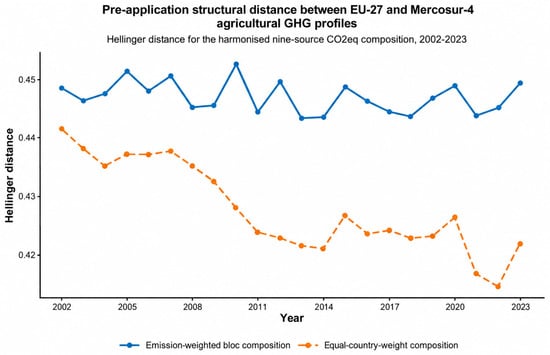
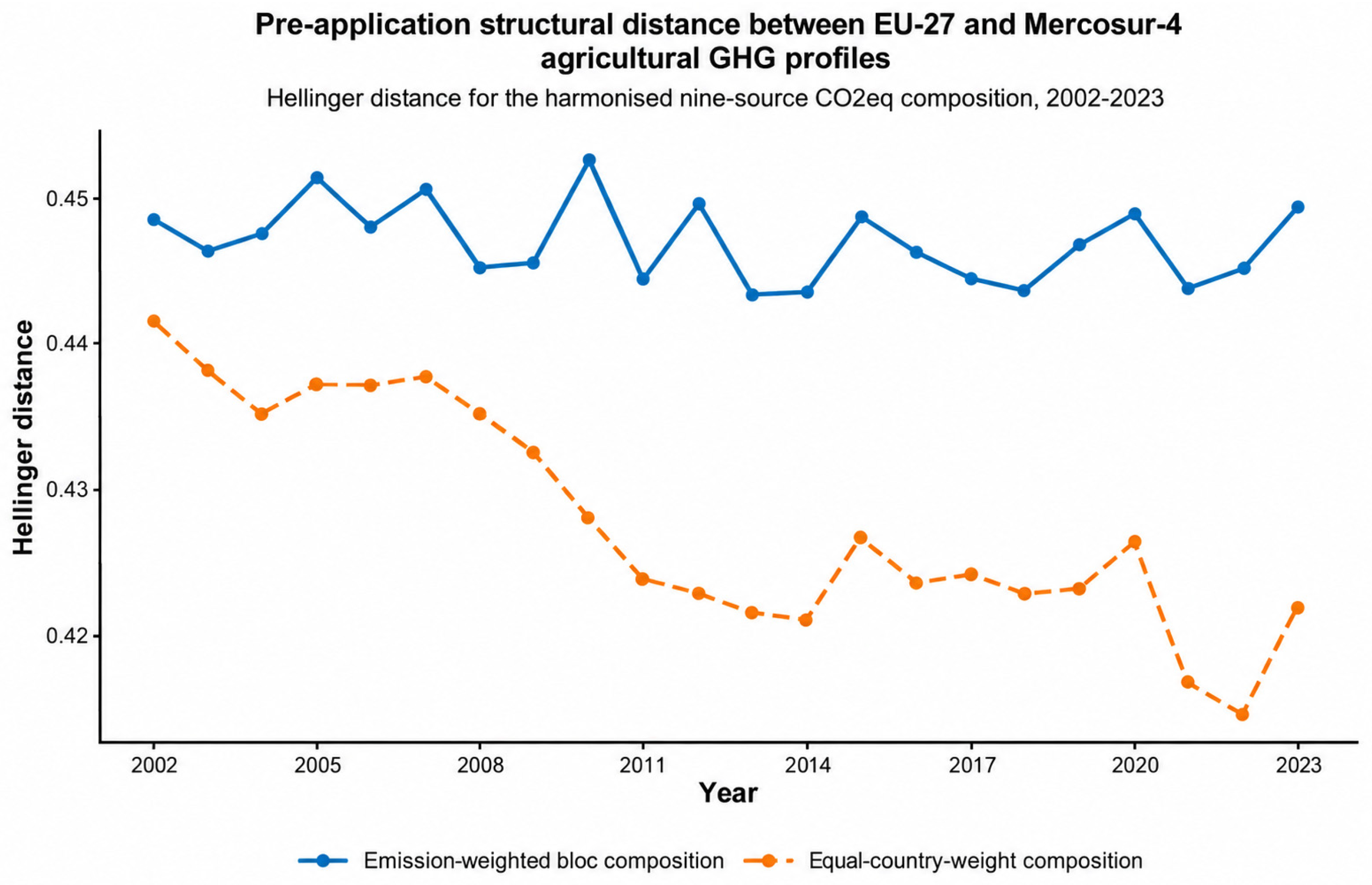

Disclaimer/Publisher’s Note: The statements, opinions and data contained in all publications are solely those of the individual author(s) and contributor(s) and not of MDPI and/or the editor(s). MDPI and/or the editor(s) disclaim responsibility for any injury to people or property resulting from any ideas, methods, instructions or products referred to in the content. |
© 2026 by the author. Licensee MDPI, Basel, Switzerland. This article is an open access article distributed under the terms and conditions of the Creative Commons Attribution (CC BY) license.