A Correction for the Cylinder Wall Adsorption in Forensic Ethanol Gas Standards

Abstract

Forensic ethanol gas standards are used for, among other things, the calibration and metrological verification of evidential breath analysers as described in OIML-R126 Evidential breath analysers. A correction for the amount fraction of ethanol in forensic gas standards due to cylinder wall adsorption is described. The correction was developed for both the national primary measurement standards as well as for derived primary reference materials. A novel method based on the well-known decanting principle was developed and assessed using two suites of gas mixtures with ethanol amount fractions between 50 μmol mol⁻¹ to 1000 μmol mol⁻¹ in nitrogen. From the results, it is inferred that the initial adsorption loss is a function of the amount fraction, and an interpolation formula was developed accordingly. To account for differences in adsorption between cylinders, a mixed-effects model was used to describe the adsorption loss data with an excess standard deviation to account for between-cylinder effects.

1. Introduction

Forensic ethanol standards play an important role in enforcing the legislation concerning driving under the influence of alcohol. In many countries, the base document for the metrological requirements for evidential breath analysis is OIML-R126 [1]. Gaseous certified reference materials (CRMs) are required to calibrate equipment that is being used for surveillance. These CRMs are generally certified for the amount fraction of ethanol in nitrogen or air. VSL, the national metrology institute of the Netherlands, maintains primary measurement standards, primary standard gas mixtures (PSMs) in the range 50 μmol mol⁻¹ to 1000 μmol mol⁻¹. The preparation of such mixtures is usually done in accordance with ISO 6142 [2,3]. The previous edition of this standard (ISO 6142:2001) [4] was amended to include the use of syringes or other transfer vessels to prepare mixtures involving liquids [5].

Currently, ISO 6142-1 [6] is widely used for preparing PSMs and primary reference materials (PRMs) for forensic ethanol gas standards. The calculation of the amount fraction of ethanol in the calibration gas mixture rests on the assumption that the composition of the constituents entered into the cylinder is identical to the composition of the (homogenised) gas mixture when sampling from the cylinder. For ethanol, this assumption is not entirely valid, as this component shows adsorption on the cylinder wall. As a result, the amount fraction of ethanol in the gas withdrawn from the cylinder is lower than the amount fraction of ethanol computed from the preparation data. As all gas molecules show some degree of adsorption on solid surfaces, this assumption is more appropriate for some types of calibration gas mixtures than for others. Ethanol, just like other polar molecules (e.g., water, ammonia), shows substantial adsorption on the cylinder wall. Whether such adsorption is problematic with respect to assigning a value and uncertainty to the amount fraction of the component of interest depends on the user requirements. For forensic ethanol standards, the adsorption is large enough to be taken into consideration given the typical uncertainty.

The PSMs of National Metrology Institutes (NMIs) are compared in key comparisons to assess their equivalence [7,8]. In the key comparison CCQM-K4 [2], the values and uncertainties assigned to the amount fraction of ethanol were just those obtained from the preparation process of ISO 6142 [4,5]. In the next key comparison, CCQM-K93, however, some NMIs applied an adsorption correction, whereas others did not. VSL was among the latter. The nominal value of the amount fraction of ethanol in CCQM-K93 was 120 μmol mol⁻¹. The travelling standards submitted were used as a calibration standard, and the result of the amount fraction of a working standard was recorded [3]. A consensus value was used to evaluate the results of the key comparison. Considering this design of CCQM-K93, a positive difference in the degree of equivalence flags that the amount fraction of ethanol in the travelling standard assigned was too high. That is consistent with an unaccounted loss of ethanol due to cylinder wall adsorption.

The aim of this work is to develop a method for measuring the adsorption loss when preparing a calibration gas mixture in a cylinder with a given type of passivation. Passivation of the interior of a gas cylinder serves the purpose of reducing the reactivity and adsorption of molecules at the cylinder wall. It should be borne in mind that the effects are usually reduced, rather than completely eliminated. Generally, it is believed that the adsorption of a component at a surface is a function of the temperature, pressure and composition of the gas mixture [9]. It is not considered a function of the preparation process, or the order in which the materials are transferred into the cylinder. Depending on this order, it may take shorter or longer to equilibrate and homogenise the calibration gas mixture after preparation. This equilibration also involves the equilibrium between adsorbed molecules and molecules of the same entity in the gas or vapour phase.

The experimental details of the method are described in Section 2. The modelling of the adsorption loss is described in Section 3 and the data reduction methods in Section 4. The results are summarised in Section 5. Form these, an interpolation formula was developed, as described in Section 6, which is aimed at predicting the adsorption loss of ethanol in these standards in cylinders with nominally the same cylinder passivation and equipped with the same valve.

2. Experimental

The method for measuring the adsorption losses used decanting of a gravimetrically prepared ethanol standard into a nominally identical, evacuated gas cylinder [9,10,11]. Using cylinders having the same passivation and valve, it is assumed that the loss that occurs during the gravimetric gas mixture preparation also occurs during decanting.

The parent gas mixtures were prepared in accordance with ISO 6142-1 [6] using the syringe method. Cylinders were chosen that had not contained ethanol in nitrogen mixtures previously. The cylinders had been flushed with high-purity nitrogen and evacuated eight times. The preparation process was described previously elsewhere [12]. For the weighing of the cylinder and the syringe, the substitution method was used [13]. This method ensures that the environmental effects of weighing the syringe and gas cylinder are mostly compensated. The method is employed with conventional mass, which is fit for purpose for high-accuracy gas mixture preparation using static gravimetry. After preparation, the cylinder containing the mixture was homogenised using a mechanical roller for 1 h.

The decanted samples were prepared using evacuated gas cylinders that underwent the same flushing procedure using high-purity nitrogen and evacuation. For decanting, the same process is used for preparing calibration gas mixtures with adsorbing or reactive components. Features of this method are the use of a heated (70 °C), short transfer line, and using a flow rate that does not exceed 1 g min⁻¹ of the gas transferred from the parent gas cylinder. This process mitigates losses during the transfer of the parent gas mixture to the cylinder for the child mixture. After preparation, the cylinder containing the mixture was homogenised using a mechanical roller for 1 h.

The assumption that the adsorption loss in the decanted mixture is expected to be the same as for the parent mixture further rests on the long-term experience that the amount fraction of ethanol in almost depleted PSMs does not differ significantly from that from freshly made PSMs, so the filling pressure seems to be of less importance, down to the threshold of 1 MPa. Below this minimum utilisation pressure [6,9,14], which is also stated on the certificates of disseminated PRMs, the amount fraction of ethanol increases.

Two sets of mixtures were prepared, see Table 1 and Table 2. The stated uncertainties are those from gravimetric preparation only, and do not account for, e.g., adsorption losses and the verification of the mixtures. The amount fractions for the second set were chosen to be slightly different, so that when the two data sets were combined in the regression, the relationship between the adsorption loss ($\delta$) and the amount fraction of ethanol (x) could be better established. It had been anticipated that between-cylinder effects would play a more important role at low amount fractions and the behaviour of the passivation would be more regular for amount fractions above 100 μmol mol⁻¹.

Table 1. Mixtures set #1 with the amount fractions ethanol (x) and standard uncertainties ($u\mathbf{\left(}x\mathbf{\right)}$) in μmol mol⁻¹ as calculation from gravimetric gas mixture preparation.

Parent	Child	x	$\mathit{u} \left(\mathit{x}\right)$
VSL348581	VSL348894	49.815	0.014
VSL447826	VSL265181	79.784	0.013
VSL348513	VSL387539	99.849	0.021
VSL247340	VSL328603	125.062	0.021
VSL249697	VSL348538	200.111	0.014
VSL323534	VSL347753	398.434	0.022
VSL338372	VSL438387	678.606	0.030
VSL409605	VSL449654	999.420	0.038

Table 2. Mixtures set #2 with the amount fractions of ethanol (x) and standard uncertainties ($u\left(x\right)$) in μmol mol⁻¹ as a calculation from gravimetric gas mixture preparation.

Parent	Child	x	$\mathit{u} \mathbf{\left(}\mathit{x}\mathbf{\right)}$
VSL291407	VSL244124	49.620	0.013
VSL338580	VSL244178	100.062	0.012
VSL265081	VSL444218	125.264	0.014
VSL600684	VSL244189	199.650	0.018
VSL349709	VSL243523	399.299	0.018
VSL386097	VSL244707	599.395	0.022
VSL243696	VSL344181	796.617	0.029
VSL448231	VSL244471	999.138	0.037

The pairs of the parent and child mixtures were then analysed. For this purpose, an Xendos 2500 non-dispersive infrared spectroscopy (NDIR) analyser from Servomex was used that is normally used for verification measurements as described in ISO 6142-1 [6] and is used for calibrating gas mixtures using ISO 6143 [15]. This method is part of the regular procedures for creating PSMs and PRMs. The performance of this method is documented elsewhere [16]. The cylinders were connected using dedicated stainless steel regulators. The measurements were performed by connecting the suite of 16 gas mixtures to a 16-way multi-position valve, which in turn was connected to the NDIR monitor. The mixtures were analysed from low to high amount fraction, and the child before the parent in the sequence. The flushing of the regulators and sampling lines was done as usual.

The NDIR analyser was operated in the same way as during such verification measurements and calibrations. For each mixture, a response was obtained by sampling the signal for 90 s, providing 90 indications. From these indications, a mean and standard deviation were computed, which are used as the response and standard uncertainty of the response, respectively. The characterisation of this kind of analyser has revealed that the noise of the signal is not white noise, so the assumption that the 90 indications are independent and identically distributed (IID) and Gaussian is not appropriate here. The chosen approach provides a cautious value for the standard uncertainty, assuming a high degree of (auto)correlation [17] between the 90 indications.

During the analysis of the set of mixtures in Table 1, it was noted that the amount fraction assigned based on the gravimetric gas mixture preparation was off for the nominally 700 μmol mol⁻¹ mixture. The same effect was visible in the data for the child. It was decided that instead of discarding the data, re-assign the amount fraction of ethanol based on the first analysis. A straight line was used as a calibration function, and the data from the parent mixtures were processed in accordance with ISO 6143 [15]. The amount fraction used for VSL338372 was, based on the analysis, adjusted to 678.606 μmol mol⁻¹ with a standard uncertainty of 0.030 μmol mol⁻¹. The latter standard uncertainty does not include any adsorption aspects.

For each of the gas mixtures indexed $i=1,\dots ,8$, five measurements were taken indexed $j=1,\dots ,5$ consisting of three runs indexed $k=1,2,3$. The gas mixtures of the second suite are indexed $i=9,\dots ,16$. The adsorption correction ${\delta }_{ijk}$ is calculated for each run of each measurement for each gas mixture pair to obtain an adsorption correction ${\widehat{\widehat{\delta }}}_i$ for each of the 16 pairs of gas mixtures.

3. Adsorption Correction

The relationship between adsorption loss, amount fraction ethanol and the responses was developed using the model for a single-point calibration [18,19]. In usual calibrations, a straight line is used as a calibration function, and as the instrument response is corrected for a zero offset, the straight line passes in good approximation through the origin [16], no non-linearity effect of the analyser had to be taken into account. Considering that the anticipated losses are in the order of 0.2 μmol mol⁻¹ to 10 μmol mol⁻¹, the departure from a straight line through the origin between parent and child is expected to be negligible in relation to other uncertainty components.

An important assumption underlying the modelling is that the adsorption of ethanol in two nominally identical cylinders with the same passivation and valves is the same. So, it is expected that the parent calibration gas mixtures are prone to a single adsorption loss, whereas the children are expected to have a double adsorption loss. Deviations from this assumption add to the between-cylinder standard deviation and affect the estimates of the adsorption loss. In practice, gravimetrically prepared ethanol in nitrogen mixtures will not become PSMs or PRMs if the adsorption is too large. Then, the gas mixture will not pass the verification test [6,15] and be rejected.

The adsorption loss is modelled to the observed responses as follows. Let the response factor be defined as

$$r_{ijk}={\displaystyle \frac{y_{ijk}}{x_i}},$$

(1)

where $y_{ijk}$ denotes the instrument response and $x_i$ the amount fraction of ethanol. If there is adsorption from ethanol to the wall, then the corrected amount fraction $x_i^{\prime }$ will be smaller than $x_i$ by a difference ${\delta }_i$. When decanting the mixture into an evacuated cylinder, the amount fraction $x_i^{″}$ will be smaller than $x_i$ by $2{\delta }_i$. If $r_{ijk}$ remains constant, then

$$\begin{array}{cc}\hfill y_{ijk}^{\prime }& =r_{ijk}{x}_i^{\prime },\hfill \\ \hfill y_{ijk}^{″}& =r_{ijk}{x}_i^{\prime \prime },\hfill \end{array}$$

where the corresponding responses $y_{ijk}^{\prime }$ and $y_{ijk}^{″}$ are observable. So, now a system of two equations remains with two unknowns, $r_{ijk}$ and ${\delta }_{ijk}$. $x_i$ is known from gravimetric gas mixture preparation. Considering that $x_i^{\prime }=x_i-{\delta }_i$ and $x_i^{″}=x_i-2{\delta }_{ijk}$, the responses can be expressed as

$$\begin{array}{cc}\hfill y_{ijk}^{\prime }& =r_{ijk}(x_i-{\delta }_{ijk}),\hfill \end{array}$$

(2)

$$\begin{array}{cc}\hfill y_{ijk}^{″}& =r_{ijk}(x_i-2{\delta }_{ijk}).\hfill \end{array}$$

(3)

Subtracting Equation (3) from Equation (2) yields

$$y_{ijk}^{\prime }-y_{ijk}^{″}=r_{ijk}{\delta }_{ijk},$$

(4)

and the response factor $r_{ijk}$ can be computed from

$$y_{ijk}^{\prime }=r_{ijk}{x}_i-(y_{ijk}^{\prime }-y_{ijk}^{″}),$$

using Equations (2) and (4). Finally,

$$r_{ijk}={\displaystyle \frac{2y_{ijk}^{\prime }-y_{ijk}^{″}}{x_i}}.$$

(5)

${\delta }_{ijk}$ can now be computed as (see also Equation (4))

$${\delta }_{ijk}={\displaystyle \frac{y_{ijk}^{\prime }-y_{ijk}^{″}}{2y_{ijk}^{\prime }-y_{ijk}^{″}}}{x}_i.$$

(6)

This correction can be related to the mass of ethanol transferred into the cylinder by using the formulæ of ISO 6142-1 [6,20], but can also be applied directly to the amount fraction computed from gravimetric gas mixture preparation. It is worth noting that Equation (6) expresses the drop in the amount fraction of ethanol solely in the observable responses of the parent and child calibration gas mixtures and the amount fraction assigned on the basis of the gravimetric preparation.

For physical reasons, values for ${\delta }_{ijk}$ can be restricted to be non-negative and not exceed $x_i$. If all molecules were adsorbed onto the surface, it is expected that the amount fraction in the gas phase would be zero, so the adsorption loss equals the amount fraction as calculated from preparation. For ethanol, the constraint is that values for ${\delta }_{ijk}$ may not have too much influence, as for this molecule, there is appreciable adsorption. For molecules with weaker interactions, such as carbon dioxide or methane, including this constraint in data models can be appropriate. For this study, the constraint that ${\delta }_{ijk}$ is non-negative did not need to be enforced. The measured values and uncertainties were such that these results were all significantly greater than zero.

One of the traits of this method is that it is straightforward to combine results from different experiments. It is assumed that pairs of mixtures (parent/child) are always analysed under repeatability conditions. Working under repeatability conditions provides the smallest uncertainties for the adsorption losses ${\delta }_i$. Combining the results from different pairs does not rest on working under repeatability conditions though. Thus, it is straightforward to combine the results from different series of experiments.

4. Data Reduction

To obtain a representative value for the adsorption loss for each pair of gas mixtures, the data obtained using the method described in Section 2 were reduced in two steps using a Bayesian hierarchical model. This model originates from the literature [21,22] and is used in several applications in metrology, including the reduction of data in key comparisons [23,24]. The model is based on a likelihood function that assumes the data to be normally distributed conditional on the mean and variance, and uses weakly informative priors for the three parameters: the mean, the between-group standard deviation and the within-group standard deviation.

The data reduction was performed in two steps. In the first step, the adsorption loss ${\overline{\delta }}_{ij}$ for measurement j of cylinder pair i was obtained as the mean of the results of the three runs. The likelihood takes the form [21]

$${\delta }_{ijk}|{\overline{\delta }}_{ij},{\tau }_{\mathrm{r},ij},{\sigma }_{\mathrm{r},ij}\sim \mathcal{N}({\overline{\delta }}_{ij},{\tau }_{\mathrm{r},ij}^2+{\sigma }_{\mathrm{r},ij}^2),$$

where ${\overline{\delta }}_{ij}$ denotes the mean of the runs, ${\tau }_{\mathrm{r},ij}$ the between-run standard deviation and ${\sigma }_{\mathrm{r},ij}$ the within-run standard deviation. The latter two parameters are needed to model the uncertainty about the results from the runs duly, and acknowledge that there can be a meaningful between-run standard deviation. It is assumed that the within-run standard deviation is the same for all runs, so this standard deviation is pooled. The weakly informative priors are specified as

$$\begin{array}{cc}\hfill {\overline{\delta }}_{ij}& \sim \mathcal{N}({\mu }_{\mathrm{r},0,i},{\left({\mu }_{\mathrm{r},0,i}\right)}^2),\hfill \\ \hfill {\tau }_{\mathrm{r},ij}& \sim \mathrm{Cauchy}(0,{\tau }_{\mathrm{r},0,i}),\hfill \\ \hfill {\sigma }_{\mathrm{r},ij}& \sim \mathrm{Cauchy}(0,{\sigma }_{\mathrm{r},0,i}),\hfill \end{array}$$

where Cauchy denotes the half Cauchy distribution [21,25,26]. None of these priors contains much information. They were chosen so that the Markov Chain Monte Carlo method (MCMC) samples from the regions with likely values for the parameters in the Bayesian hierarchical model [21,27]. The parameters for the prior probability distribution functions for fitting the data from the runs for the first set of mixtures are shown in Table 3. The scale parameters ${\tau }_{\mathrm{r},0}$ and ${\sigma }_{\mathrm{r},0}$ for the Cauchy distribution have been chosen in accordance with the description in [26]. The normal prior for the adsorption correction has been chosen with a mean to be close to the anticipated adsorption losses and a standard deviation that equals the mean, thereby obtaining a weakly informative prior. The purpose of the latter prior is to improve the performance of the MCMC. For the second set of mixtures, the priors are given in Table 4.

Table 3. Parameters of the prior distributions for the first set of mixtures (μmol mol⁻¹).

Level	${\mathit{\mu }}_{\mathbf{r},0}$	${\mathit{\tau }}_{\mathbf{r},0}$	${\mathit{\sigma }}_{\mathbf{r},0}$
1	0.50	0.05	0.10
2	0.50	0.20	0.10
3	0.50	0.20	0.10
4	0.50	0.20	0.10
5	2.00	0.20	0.10
6	2.00	0.50	0.10
7	3.00	0.50	0.10
8	5.00	0.50	0.10

Table 4. Parameters of the prior distributions for the second set of mixtures (μmol mol⁻¹).

Level	${\mathit{\mu }}_{\mathbf{r},0}$	${\mathit{\tau }}_{\mathbf{r},0}$	${\mathit{\sigma }}_{\mathbf{r},0}$
1	0.50	0.10	0.10
2	0.50	0.20	0.10
3	0.50	0.20	0.10
4	0.80	0.20	0.10
5	1.00	0.20	0.10
6	2.00	0.30	0.10
7	3.00	0.30	0.10
8	8.00	0.30	0.10

The model was fitted using MCMC as implemented in R (version 4.4.2) [28] using the RStan package [29]. Four (4) chains were used, the number of iterations 300,000 of which 50,000 were used as ‘burn-in’. No thinning was used.

The adsorption losses of the five measurements were combined with a Bayesian hierarchical model with a very similar specification. As data, the estimates for ${\overline{\delta }}_{ij}$ were used, together with their associated standard deviations as obtained from the first stage. The likelihood of the second stage takes the form

$${\overline{\delta }}_{ij}|{\overline{\overline{\delta }}\delta }_i,{\tau }_{\mathrm{m},i},{\sigma }_{\mathrm{m},i}\sim \mathcal{N}({\overline{\overline{\delta }}}_i,{\tau }_{\mathrm{m},i}^2+{\sigma }_{\mathrm{m},i}^2),$$

(7)

where ${\overline{\overline{\delta }}}_i$ denotes the mean, ${\tau }_{\mathrm{m},i}$ the between-measurement standard deviation and ${\sigma }_{\mathrm{m},i}$ the within-measurement standard deviation. The latter two parameters are needed to model the uncertainty about the results from the measurements duly, and acknowledge that there can be a meaningful between-measurement standard deviation. It is assumed that the within-measurement standard deviation is the same for all measurements, so this standard deviation is pooled. The priors are specified as

$$\begin{array}{c}{\overline{\overline{\delta }}}_i\sim \mathcal{N}({\mu }_0,{\left({\mu }_0\right)}^2),\hfill \\ {\tau }_{\mathrm{m}}\sim \mathrm{Cauchy}(0,{\tau }_0),\hfill \\ {\sigma }_{\mathrm{m}}\sim \mathrm{Cauchy}(0,{\sigma }_0),\hfill \end{array}$$

where μ₀ = 5 μmol mol⁻¹, τ₀ = 0.5 μmol mol⁻¹ and σ₀ = 0.02 μmol mol⁻¹. This Bayesian model was fitted with the same settings for the MCMC as the model used to obtain the means of the runs.

5. Results

5.1. First Suite of Gas Mixtures

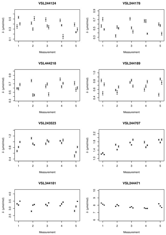
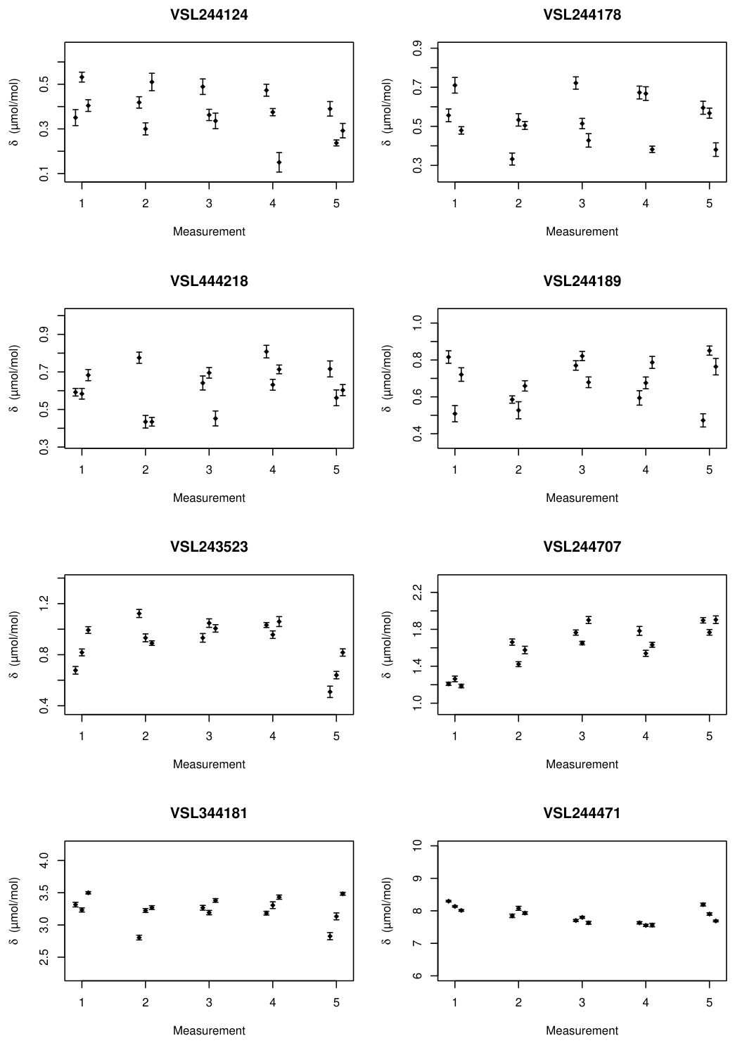
The results of measuring the adsorption losses of the first suite of pairs of gas mixtures are shown in Figure 1. Five measurements were taken, each consisting of three runs. The results of the runs are displayed from left to right in the order they were taken. The uncertainty bars indicate expanded uncertainties ($k=2$). These uncertainties were calculated by propagating the uncertainties from the monitor response and those from the gravimetric preparation of the parent gas mixtures. The mixture codes at the top of the figures correspond to the parent gas mixtures listed in Table 1.

Figure 1. Adsorption losses for the first suite of eight mixtures. The uncertainty bars indicate expanded uncertainties.

The results in Figure 1 show good consistency between runs and measurements. There is overdispersion in all data sets, hence the use of a hierarchical model with a variable to model the excess standard deviation ($\tau$). Using the hierarchical model presented in Section 4, first the runs and then the means of the five measurements, ensures that the overdispersion is properly modelled and duly propagated to the standard uncertainty computed for the adsorption loss $\delta$. This adsorption loss is the mean of all results in each of the panels in Figure 1.

The results of the five measurements are fitted using the Bayesian hierarchical model as specified previously. The same probability density functions were used as priors, but now with parameters μ₀ = 5 μmol mol⁻¹, τ₀ = 0.5 μmol mol⁻¹ and σ₀ = 0.02 μmol mol⁻¹.

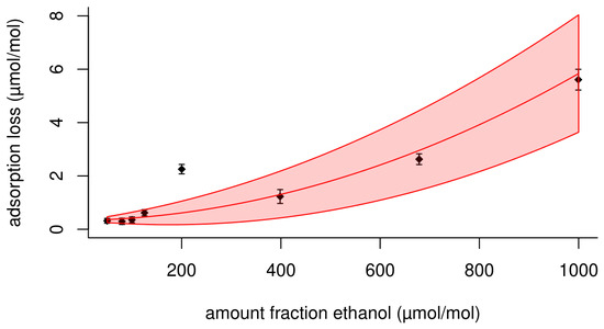
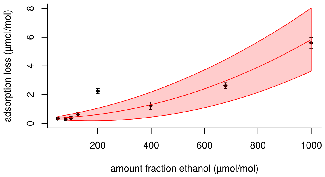
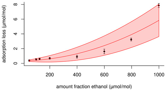
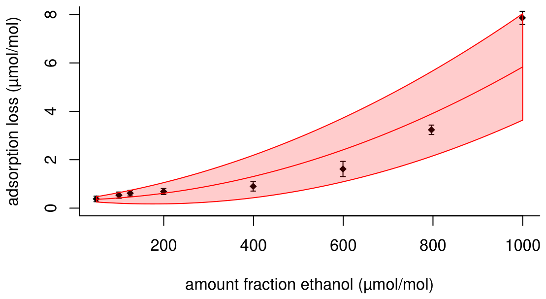
The measured adsorption losses are shown in Figure 2. The error bars indicate the standard uncertainties as obtained from fitting the second Bayesian hierarchical model, multiplied by a coverage factor $k=2$ to obtain expanded uncertainties. Form the data, it is seen that the adsorption loss is a a function of the amount fraction of ethanol. The relationship shows some curvature, but in rough approximation it can be described by a straight line. The results up to 125 μmol mol⁻¹ indicate that there is some variability between the results that appears to exceed the experimental measurement uncertainty from determining the adsorption loss (Table 5).

Figure 2. Adsorption losses and expanded uncertainties for the first set of mixtures. Solid curve and the shaded area indicate the interpolation function for the adsorption loss and the 95% coverage interval.

Table 5. Adsorption losses of the first set of mixtures (μmol mol⁻¹).

x	$\overline{\overline{\mathit{\delta }}}$	$\mathit{s} \mathbf{(}\overline{\overline{\mathit{\delta }}}\mathbf{)}$	${\mathit{\tau }}_{\mathbf{m}}$	$\mathit{s} \mathbf{\left(}{\mathit{\tau }}_{\mathbf{m}}\mathbf{\right)}$	${\mathit{\sigma }}_{\mathbf{m}}$	$\mathit{u} \mathbf{\left(}{\mathit{\sigma }}_{\mathbf{m}}\mathbf{\right)}$
49.815	0.317	0.045	0.061	0.057	0.055	0.009
79.784	0.296	0.058	0.074	0.070	0.077	0.012
99.849	0.354	0.055	0.066	0.064	0.075	0.012
125.062	0.619	0.058	0.064	0.065	0.091	0.015
200.111	2.253	0.089	0.163	0.098	0.059	0.010
398.434	1.229	0.130	0.164	0.142	0.195	0.031
678.606	2.627	0.101	0.112	0.106	0.161	0.026
999.420	5.609	0.194	0.304	0.214	0.229	0.036

The pair of mixtures at 200 μmol mol⁻¹ stands out; the adsorption loss is much larger than for the other seven pairs, considering the nominal amount fractions. This issue was already known, for in previous experiments in 2016, also a pair of mixtures was set aside in the evaluation, for the adsorption loss measured was deemed to be unrepresentative. This data set was, however, much smaller than the ones in this study, and also the range of amount fractions targeted did not match with the PSMs maintained. The results from this study, using the modelling described in Section 3, show agreement with the results presented.

5.2. Second Suite of Gas Mixtures

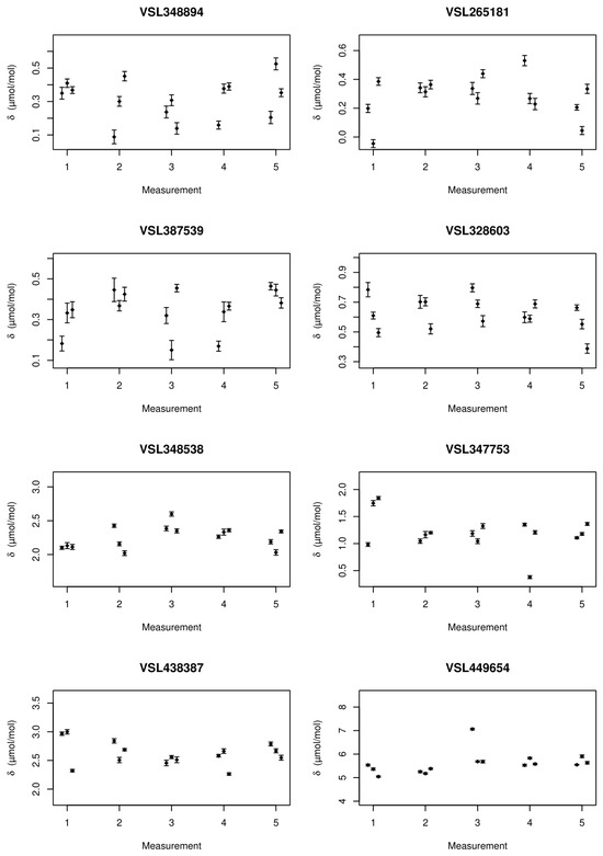
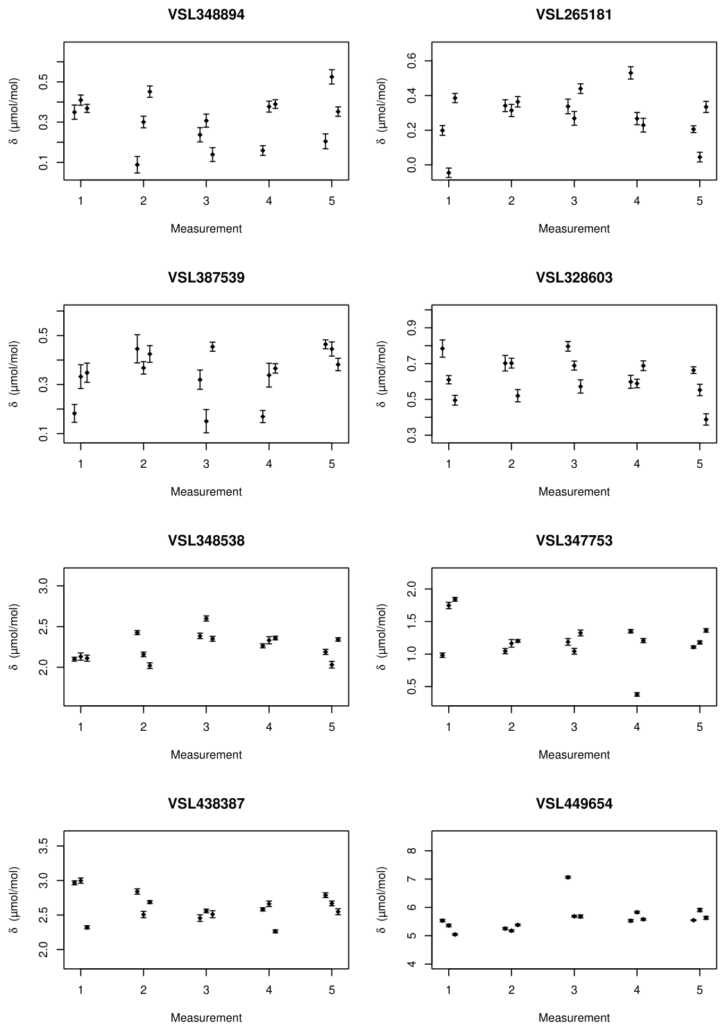
To supplement the data from the first suite of mixtures, a second suite of 8 mixtures was prepared. The nominal amount fractions of ethanol were chosen slightly differently from the first suite to provide, in the end, better support for an empirical relationship between the adsorption loss $\delta$ and the amount fraction x. The results of measuring the adsorption losses of the second suite of pairs of gas mixtures are shown in Figure 3. Five measurements were taken, each consisting of three runs. The results of the runs are displayed from left to right in the order they were taken. The uncertainty bars indicate expanded uncertainties ($k=2$). The mixture codes at the top of the figures correspond to the parent gas mixtures listed in Table 2.

Figure 3. Adsorption losses for the second suite of eight mixtures. The uncertainty bars indicate expanded uncertainties.

The results in Figure 3 show good consistency between runs and measurements. There is overdispersion in all data sets. Using the hierarchical model presented in Section 4 like was done for the first dataset, ensures that this overdispersion is properly modelled and duly propagated to the standard uncertainty computed for the adsorption loss $\delta$. This adsorption loss is the mean of all results in each of the panels in Figure 3.

The parameters for the prior probability distribution functions for the parameters in the hierarchical Bayesian model for fitting the data from the second set of mixtures are shown in Table 4. The deliberations for the choice of these values were the same as for the first set of mixtures. The adsorption losses are shown in Table 2.

The measured adsorption losses are shown in Figure 4. As in the case of Figure 2, the error bars indicate the standard uncertainties as obtained from fitting the second Bayesian hierarchical model, multiplied by a coverage factor $k=2$ to obtain expanded uncertainties. The dependence of the adsorption loss on the amount fraction for the second set of mixtures resembles that of the first set (see Figure 2). The pair of mixtures at 200 μmol mol⁻¹ of the second set fits much better in the overall trend of the adsorption losses (Table 6).

Figure 4. Adsorption losses and expanded uncertainties for the second set of mixtures. Solid curve and the shaded area indicate the interpolation function for the adsorption loss and the 95% coverage interval.

Table 6. Adsorption losses of the second set of mixtures (μmol mol⁻¹).

x	$\overline{\overline{\mathit{\delta }}}$	$\mathit{s} \mathbf{(}\overline{\overline{\mathit{\delta }}}\mathbf{)}$	${\mathit{\tau }}_{\mathbf{m}}$	$\mathit{s} \mathbf{\left(}{\mathit{\tau }}_{\mathbf{m}}\mathbf{\right)}$	${\mathit{\sigma }}_{\mathbf{m}}$	$\mathit{u} \mathbf{\left(}{\mathit{\sigma }}_{\mathbf{m}}\mathbf{\right)}$
49.620	0.379	0.058	0.059	0.069	0.078	0.013
100.062	0.535	0.065	0.069	0.070	0.106	0.018
125.264	0.618	0.058	0.067	0.066	0.088	0.015
199.650	0.685	0.062	0.069	0.069	0.097	0.016
399.299	0.899	0.097	0.158	0.114	0.100	0.016
599.395	1.616	0.157	0.290	0.158	0.107	0.017
796.617	3.236	0.098	0.109	0.103	0.158	0.026
999.138	7.863	0.137	0.234	0.150	0.127	0.021

6. Interpolation Formula

Rather than working with the measured adsorption losses themselves, for daily use it would be convenient to have an interpolation formula that predicts the adsorption loss $\delta$ for a given amount fraction of ethanol. Looking at the adsorption loss data in Figure 2 and Figure 4, it is evident that a straight line will not do to describe the data. The shape of the relationship looks more like an exponential or a quadratic function. Considering that the departure from a straight-line relationship is not too large, a quadratic function can be probed, which is mathematically easier to handle in regression than an exponential function. Furthermore, when writing the exponential function as a Taylor series, it is a polynomial [30] and it can be shown for the adsorption loss data that the terms after the quadratic term are irrelevant to describe the data. So, the relationship between $\overline{\overline{\delta }}$ and x can be written as

$${\overline{\overline{\delta }}}_i={\alpha }_1+{\alpha }_2{x}_i+{\alpha }_3{x}_i^2$$

(8)

Fitting the data from set 1 using ordinary least-squares method (OLS) provided ${\widehat{\alpha }}_1=0.35994$, ${\widehat{\alpha }}_2=-1.17\times {10}^{-4}$ and ${\widehat{\alpha }}_3=5.33\times {10}^{-6}$, where both ${\overline{\overline{\delta }}}_i$ and $x_i$ are in μmol mol⁻¹. Setting a 95% coverage interval of ±0.2% of the amount fraction of ethanol, the relative differences using the coefficients from set 1 are as follows (Table 7). The relative difference, calculated as $d_{\mathrm{rel}}=(\widehat{\delta }-\overline{\overline{\delta }})/\left(0.002x\right)$ takes values $\pm 1$ for the predicted adsorption losses within the coverage interval, save the mixture pair at 200 μmol mol⁻¹. For the second set, the parameter values from fitting the data of the first set make predictions within the same coverage interval (see Table 7). The poor prediction of the 200 μmol mol⁻¹ pair from the first set (top half of Table 7) is due to the anomalous behaviour of this pair of mixtures; the prediction for the 200 μmol mol⁻¹ pair from the second set is good. The 1000 μmol mol⁻¹ mixture pair from the second set lies just outside the 95% coverage interval from set 1.

Table 7. Measured ($\overline{\overline{\delta }}$) and predicted adsorption losses ($\widehat{\delta }$) and differences relative to 0.2% x.

x	$\overline{\overline{\delta }}$	$\widehat{\mathit{\delta }}$	${\mathit{d}}_{\mathbf{rel}}$
μmol mol−1	μmol mol−1	μmol mol−1
49.815	0.316	0.367	0.51
79.784	0.297	0.384	0.55
99.849	0.354	0.401	0.24
125.062	0.617	0.429	−0.76
200.111	2.254	0.550	−4.26
398.434	1.228	1.160	−0.08
678.606	2.625	2.735	0.08
999.420	5.601	5.563	−0.02
49.620	0.380	0.367	−0.13
100.062	0.535	0.401	−0.67
125.264	0.617	0.429	−0.75
199.650	0.684	0.549	−0.34
399.299	0.899	1.164	0.33
599.395	1.619	2.205	0.49
796.617	3.237	3.648	0.26
999.138	7.861	5.560	−1.15

For practical purposes, the uncertainty associated with the $x_i$ from gravimetric gas mixture preparation can be neglected; it is much smaller than the uncertainty associated with the ${\overline{\overline{\delta }}}_i$, so for fitting the data, the choice is between OLS or weighted least-squares method (WLS). With OLS, all data points get the same weight, which presumes that the regression data are homoscedastic (i.e., have a constant variance). Looking at the data in Figure 2 and Figure 4 shows that the standard uncertainty associated with ${\overline{\overline{\delta }}}_i$ increases with increasing $x_i$, which makes WLS the preferred choice, as it weighs the residuals according to the standard uncertainty associated with the dependent variable (here ${\overline{\overline{\delta }}}_i$).

Apart from the heteroscedasticity in the adsorption loss data, there is also an overdispersion in the data, i.e., there is more dispersion in the data than accounted for by evaluating the standard uncertainty associated with the adsorption loss. Looking at the pair at 200 μmol mol⁻¹ and 1000 μmol mol⁻¹, this overdispersion is likely to be due to the fact that the adsorption loss is not identical for each cylinder. This is a form of between-bottle homogeneity [31] and a relevant component in the evaluation of the uncertainty.

The regression method of choice should not only provide the values for the coefficients, but also a value for the standard deviation for overdispersion. Mixed-effects models, as known from meta-analysis [32] are capable of doing so. If it is assumed that the excess standard deviation is proportional to the fraction of ethanol, the regression can be performed by fitting ${\delta }_i/x_i$ as a function of $x_i$. The equation then becomes

$${\displaystyle \frac{{\delta }_i}{x_i}}={\alpha }_1{\displaystyle \frac{1}{x_i}}+{\alpha }_2+{\alpha }_3{x}_i.$$

(9)

This model was fitted in R [28] using function rma from the metafor package [33]. The weights assigned are the inverses of the squared standard uncertainties associated with the measured adsorption losses.

The coefficients of the model are given in Table 8. Considering the standard uncertainties, the coefficient ${\alpha }_2$ (the linear term) is insignificant. The value of $\tau$, the relative excess standard deviation, is 0.105%.

Table 8. Values and standard uncertainties of the coefficients of the quadratic polynomial in Equation (8) describing the adsorption loss as a function of the amount fraction ethanol.

i	${\mathit{\alpha }}_{\mathit{i}}$	$\mathit{u} \left({\mathit{\alpha }}_{\mathit{i}}\right)$
1	0.337	0.086
2	0.00028	0.00109
3	0.0000052	0.0000014

The performance of the interpolation function (8) is shown in Table 9 and Figure 5. $\widehat{\delta }$ denotes the predicted adsorption loss, $\tau$ the between-bottle effect, $u\left(\widehat{\delta }\right)$ the combination of the standard uncertainty associated with $\delta$ and the excess standard deviation $\tau$. The ultimate column in Table 9 shows the difference between the predicted and measured adsorption loss. These differences are, in absolute value, all smaller than the expanded uncertainty, obtained as twice the standard uncertainty $u\left(\widehat{\delta }\right)$.

Table 9. Measured ($\overline{\overline{\delta }}$) and predicted adsorption losses ($\widehat{\delta }$), including the between-bottle standard deviation ($\tau$) (μmol mol⁻¹).

x	$\overline{\overline{\delta }}$	$\mathit{u} (\overline{\overline{\delta }})$	$\widehat{\mathit{\delta }}$	$\mathit{\tau }$	$\mathit{u} (\widehat{\mathit{\delta }})$	$\widehat{\mathit{\delta }}-\overline{\overline{\delta }}$
49.815	0.317	0.045	0.364	0.054	0.070	0.047
79.784	0.296	0.058	0.393	0.086	0.104	0.097
99.849	0.354	0.055	0.417	0.108	0.121	0.064
125.062	0.619	0.058	0.454	0.135	0.147	−0.164
200.111	2.253	0.089	0.603	0.216	0.234	−1.651
398.434	1.229	0.130	1.279	0.430	0.450	0.051
678.606	2.627	0.101	2.936	0.733	0.740	0.309
999.420	5.609	0.194	5.839	1.080	1.097	0.230
49.620	0.379	0.058	0.364	0.054	0.079	−0.015
100.062	0.535	0.065	0.418	0.108	0.126	−0.117
125.264	0.618	0.058	0.454	0.135	0.147	−0.163
199.650	0.685	0.062	0.602	0.216	0.224	−0.084
399.299	0.899	0.097	1.283	0.431	0.442	0.384
599.395	1.616	0.157	2.384	0.648	0.666	0.768
796.617	3.236	0.098	3.879	0.861	0.866	0.642
999.138	7.863	0.137	5.836	1.079	1.088	−2.026

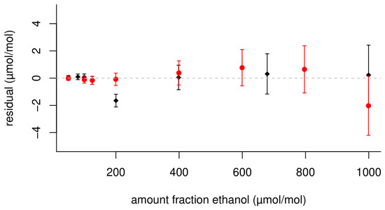
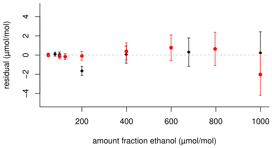
Figure 5. Residuals of fitting the adsorption losses using a quadratic polynomial and their expanded uncertainties. The dashed line indicates zero; the black diamonds refer to the first set of mixtures and the red circles to the second set.

The relative standard uncertainty associated with the correction is 0.11% for amount fractions in the range 100 μmol mol⁻¹ to 1000 μmol mol⁻¹ and increases to 0.15% for amount fractions down to 50 μmol mol⁻¹ (Table 9). The residuals are shown in Figure 5. Most of these residuals are within $\pm \tau$. The 200 μmol mol⁻¹ pair of mixtures from the first set is a notable exception. The two 1000 μmol mol⁻¹ pairs of mixtures agree reasonably well with each other.

The proposed standard uncertainty associated with the adsorption correction is given in the final column. This standard uncertainty is slightly larger than the value of $\tau$, for it includes the measurement uncertainty from the measured adsorption loss.

The residuals in Figure 5 show largely opposite signs across the range of amount fractions. For instance, for the data in the range from 50 μmol mol⁻¹ to 125 μmol mol⁻¹, the relative differences are positive in the first data set and negative in the second; also, the relative differences at 1000 μmol mol⁻¹ carry opposite signs. These patterns flag that the interpolation formula does not induce a particular bias in a specific part of the amount fraction range from 50 μmol mol⁻¹ to 1000 μmol mol⁻¹ and represents the empirical data well.

7. Discussion and Conclusions

The method used for measuring adsorption losses enables determining these losses under repeatability conditions. The link with the amount fraction of ethanol is established using the amount fraction computed from the static gravimetric preparation according to ISO 6142-1. In this case, no further calibration of the analyser was deemed necessary, as the performance characteristics of the analyser were known. From the calibration function established for the first suite of gas mixtures prepared for this study, it was inferred that the amount fraction of the 700 μmol mol⁻¹ mixture was off, which propagated to the amount fraction of ethanol in the decanted (child) mixture. Parent and child were assigned a new amount fraction based on analysis using the multipoint calibration method of ISO 6143 [15]. In all other cases, the analyser was effectively calibrated using a single-point approach according to ISO 12963 [18,19].

The method for determining the adsorption losses uses three observable quantities, i.e., the amount fraction of ethanol as computed from ISO 6142-1 [6,20], the response of the parent mixture and the response of the chlid mixture, to compute the adsorption loss. From the input quantities, further desired output quantities can be computed, such as the amount fractions of ethanol in the parent and child mixtures adjusted for the adsorption loss.

The adsorption losses are a function of the amount fraction of ethanol. From the results, a quadratic interpolation function was established. A mixed-effects model with excess variance was needed to account for the between-bottle homogeneity effects. These effects are due to the apparent differences in adsorption between gas cylinders with nominally identical passivation and cylinder values. Including the between-bottle homogeneity effect, the interpolation formula predicts adsorption losses for the amount fraction ethanol from 50 μmol mol⁻¹ to 1000 μmol mol⁻¹ with a relative standard uncertainty from 0.15% to 0.11%. Cylinders that show anomalous adsorption behaviour will be found during the verification of gravimetrically prepared ethanol standards by a result that does not agree with the result obtained from preparation, including an adjustment for the ethanol adsorption.

The work underlines that between-bottle effects in reference material production can be relevant even in cases when reference materials (RMs) are characterised and provided one at a time. This is a notion that is missed in ISO 10734 [34] and ISO 33405 [31]. For most RMs, interactions between the material and the inner surface of the packaging material (e.g., sample container) are minimal, but in gas analysis this is not necessarily the case for high-end applications. The phenomenon is, for instance, also relevant for RMs for nitrogen dioxide analysis and other reactive components. When extreme precision between RMs is required, as with RMs for monitoring greenhouse gases, between-bottle effects are also relevant to consider in the uncertainty budget(s) of the property value(s).

References

- OIML R 126; Evidential Breath Analysers. OIML, International Organization for Legal Metrology: Paris, France, 2021.
- Milton, M.J.T.; Brookes, C.; Marschal, A.; Guenther, F.; de Leer, E.; Zhen, W.L.; Takahashi, C.; Deak, E.; Kustikov, Y. Final Report of Key Comparison CCQM-K4 (Ethanol in Air); Technical Report; NPL: Teddington, UK, 2001. [Google Scholar]
- Brown, A.S.; Milton, M.J.T.; Brookes, C.; Vargha, G.M.; Downey, M.L.; Uehara, S.; Augusto, C.R.; de Lima Fioravante, A.; Sobrinho, D.G.; Dias, F.; et al. Final report on CCQM-K93: Preparative comparison of ethanol in nitrogen. Metrologia 2013, 50, 08025. [Google Scholar] [CrossRef] [Scilit]
- ISO 6142; Gas Analysis—Preparation of Calibration Gas Mixtures—Gravimetric Method. 2nd ed. ISO, International Organization for Standardization: Geneva, Switzerland, 2001.
- ISO 6142:2001/Amd 1:2009; Liquid Introduction. ISO, International Organization for Standardization: Geneva, Switzerland, 2009.
- ISO 6142–1; Gas Analysis—Preparation of Calibration Gas Mixtures—Gravimetric Method for Class I Mixtures. 1st ed. ISO, International Organization for Standardization: Geneva, Switzerland, 2015.
- CIPM. Mutual Recognition of National Measurement Standards and of Calibration and Measurement Certificates Issued by National Metrology Institutes; CIPM: Sèvres, France, 1999. [Google Scholar]
- CIPM MRA-G-11; Measurement Comparisons in the CIPM MRA. Guidelines for Organizing, Participating and Reporting. Version 1.1. Bureau International des Poids et Mesures, BIPM: Sèvres, France, 2021.
- Leuenberger, M.C.; Schibig, M.F.; Nyfeler, P. Gas adsorption and desorption effects on cylinders and their importance for long-term gas records. Atmos. Meas. Tech. 2015, 8, 5289–5299. [Google Scholar] [CrossRef] [Scilit]
- Brewer, P.J.; Kim, J.S.; Lee, S.; Tarasova, O.A.; Viallon, J.; Flores, E.; Wielgosz, R.I.; Shimosaka, T.; Assonov, S.; Allison, C.E.; et al. Advances in reference materials and measurement techniques for greenhouse gas atmospheric observations. Metrologia 2019, 56, 034006. [Google Scholar] [CrossRef] [Scilit]
- Brewer, P.J.; Brown, R.J.C.; Webber, E.B.M.; van Aswegen, S.; Ward, M.K.M.; Hill-Pearce, R.E.; Worton, D.R. Breakthrough in negating the impact of adsorption in gas reference materials. Anal. Chem. 2019, 91, 5310–5315. [Google Scholar] [CrossRef] [Scilit] [PubMed]
- van Andel, I.; van der Veen, A.M.H.; Zalewska, E.T. A robot for weighing syringes used in reference gas mixture preparation. Metrologia 2012, 49, 446. [Google Scholar] [CrossRef] [Scilit]
- International Organization of Legal Metrology. OIML R111-1 Weights of Classes E1, E2, F1, F2, M1, M1-2, M2, M2-3, and M3. Part 1: Metrological and Technical Requirements; International Bureau of Legal Metrology: Paris, France, 2004. [Google Scholar]
- ISO 6141; Gas Analysis—Contents of Certificates for Calibration Gas Mixtures. 4th ed. ISO, International Organization for Standardization: Geneva, Switzerland, 2015.
- ISO 6143; Gas Analysis—Comparison Methods for Determining and Checking the Composition of Calibration Gas Mixtures. 3rd ed. ISO, International Organization for Standardization: Geneva, Switzerland, 2025.
- van der Veen, A.M.H.; van Wijk, J.I.T. Calibration and Measurement Capabilities for Mixtures of Ethanol in Nitrogen/Synthetic Air; Technical Report; Report S-CH.21.18; VSL, Department of Chemistry: Delft, The Netherlands, 2021. [Google Scholar]
- Shumway, R.H.; Stoffer, D.S. Time Series Analysis and Its Applications: With R Examples; Springer International Publishing: Cham, Switzerland, 2017. [Google Scholar]
- ISO 12963; Gas Analysis—Comparison Methods for the Determination of the Composition of Gas Mixtures Based on One- and Two-Point Calibration. 1st ed. ISO, International Organization for Standardization: Geneva, Switzerland, 2017.
- ISO 12963:2017/Amd 1:2020; Gas Analysis—Comparison Methods for the Determination of the Composition of Gas Mixtures Based on One- and Two-Point Calibration. Amendment 1: Correction to Formula 5. 1st ed. ISO, International Organization for Standardization: Geneva, Switzerland, 2020.
- ISO 6142-1:2015/Amd 1:2020; Gas Analysis—Preparation of Calibration Gas Mixtures—Part 1: Gravimetric Method for Class I Mixtures. Amendment 1: Corrections to Formulae in Annex E and Annex G. ISO, International Organization for Standardization: Geneva, Switzerland, 2020.
- Gelman, A.; Carlin, J.; Stern, H.; Dunson, D.; Vehtari, A.; Rubin, D. Bayesian Data Analysis, 3rd ed.; Chapman and Hall/CRC: Boca Raton, FL, USA, 2013. [Google Scholar]
- Gelman, A. Objections to bayesian statistics. Bayesian Anal. 2008, 3, 445–449. [Google Scholar] [CrossRef] [Scilit]
- Koepke, A.; Lafarge, T.; Possolo, A.; Toman, B. Consensus building for interlaboratory studies, key comparisons, and meta-analysis. Metrologia 2017, 54, S34. [Google Scholar] [CrossRef] [Scilit]
- Koepke, A.; Lafarge, T.; Possolo, A.; Toman, B. NIST Consensus Builder User’s Manual; Technical Report; National Institute of Standards and Technology: Gaithersburg, MD, USA, 2016. [Google Scholar]
- Wikipedia Contributors. Cauchy Distribution—Wikipedia, the Free Encyclopedia, 2024. Available online: https://en.wikipedia.org/wiki/Cauchy_distribution (accessed on 29 October 2024).
- Gelman, A. Prior distributions for variance parameters in hierarchical models (Comment on article by Browne and Draper). Bayesian Anal. 2006, 1, 515–534. [Google Scholar] [CrossRef] [Scilit]
- van der Veen, A.M.H. Bayesian methods for type A evaluation of standard uncertainty. Metrologia 2018, 55, 670–684. [Google Scholar] [CrossRef] [Scilit]
- R Core Team. R: A Language and Environment for Statistical Computing; R Foundation for Statistical Computing: Vienna, Austria, 2025. [Google Scholar]
- Stan Development Team. RStan: The R Interface to Stan, R Package Version 2.26.11; Stan Development Team: New York City, NY, USA, 2022. Available online: https://mc-stan.org/ (accessed on 29 October 2024).
- Boas, M.L. Mathematical Methods in the Physical Sciences; John Wiley & Sons Inc.: Hoboken, NJ, USA, 2005. [Google Scholar]
- ISO 33405; Reference Materials—Approaches for Characterization and Assessment of Homogeneity and Stability. 1st ed. ISO, International Organization for Standardization: Geneva, Switzerland, 2024.
- Schwarzer, G.; Carpenter, J.R.; Rücker, G. Meta-Analysis with R (Use R!); Springer: Cham, Switzerland, 2015. [Google Scholar]
- Viechtbauer, W. Conducting meta-analyses in R with the metafor package. J. Stat. Softw. 2010, 36, 1–48. [Google Scholar] [CrossRef] [Scilit]
- ISO 17034; General Requirements for the Competence of Reference Material Producers. 1st ed. ISO, International Organization for Standardization: Geneva, Switzerland, 2016.
Disclaimer/Publisher’s Note: The statements, opinions and data contained in all publications are solely those of the individual author(s) and contributor(s) and not of MDPI and/or the editor(s). MDPI and/or the editor(s) disclaim responsibility for any injury to people or property resulting from any ideas, methods, instructions or products referred to in the content. |
© 2026 by the authors. Licensee MDPI, Basel, Switzerland. This article is an open access article distributed under the terms and conditions of the Creative Commons Attribution (CC BY) license.