


Abstract
This study aimed to identify and characterise major wildfire events in South Africa (SA) between 2004 and 2023 by integrating long-term multi-source datasets with anomaly detection techniques. Biomass-burning emissions, such as black carbon from biomass burning (BCBB), organic carbon from biomass burning (OCBB), and carbon monoxide (CO), were retrieved from the Modern-Era Retrospective Analysis for Research and Applications, Version 2 (MERRA-2) reanalysis dataset, while burned area data were obtained from the Moderate Resolution Imaging Spectroradiometer (MODIS). Isolation Forest (IF; contamination = 0.05) and the Generalised Extreme Studentised Deviate (GESD) test were applied independently and integrated at the decision level: single-method detections were classified as candidate anomalies, while agreement between the methods identified high-confidence anomalies. Calendar-month standardisation, Spearman rank correlation, Benjamini–Hochberg false-discovery-rate correction, and calendar-month-matched event composites were used to assess meteorological relationships. IF-selected 12 candidate months were identified throughout, whereas GESD identified a smaller subset. July 2007 was the only high-confidence burned area anomaly. High-confidence emission anomalies occurred in 2010, 2018, 2021, and 2023, predominantly between September and November, while the only high-confidence precipitation anomaly occurred in August 2006. After false-discovery-rate correction, the burned area was weakly associated with higher wind speed and lower daytime relative humidity. CO, BCBB, and OCBB were weakly associated with lower precipitation, lower daytime relative humidity, and higher wind speed, while surface air temperature (SAT) showed no significant relationships. Event composites displayed similar patterns, but none of the 16 comparisons remained statistically significant after correction. Spatial analyses showed that the July 2007 burned area anomaly was concentrated in eastern SA; CO and BCBB anomalies were prominent across the northern, central, and eastern interior, and the 2018 OCBB anomalies were concentrated in the southern Western Cape. Percentile-selected spatial composites demonstrated additional regional heterogeneity but were distinct from the IF-GESD consensus anomalies and were interpreted descriptively. The framework, therefore, provides transparent confidence stratification rather than evidence of superior predictive accuracy, while highlighting limitations arising from national monthly aggregation and differences in product resolution.
1. Introduction
Wildfire occurrence and behaviour arise from interactions among anthropogenic activities, meteorological conditions, vegetation characteristics and landscape properties [1]. Temperature, precipitation, wind speed and relative humidity influence fuel moisture, ignition probability, fire spread and fire intensity [2,3], while high surface temperatures, low relative humidity, drought and strong winds are especially associated with elevated fire danger and extreme wildfire conditions [3,4,5]. These meteorological influences operate alongside topography, fuel type and load, soil moisture, ignition sources and land-management practices, which further shape how fires develop across landscapes [1,6,7].
These controls operate in ecosystems where fire can be both ecologically important and environmentally damaging. Although fire contributes to nutrient cycling and vegetation succession, the increasing frequency and intensity of extreme events have raised substantial concern [8]. Severe or recurrent fires can cause long-term ecosystem degradation and, under exceptional conditions, contribute to ecosystem collapse [9]. Their effects may persist beyond immediate vegetation loss through changes in ecosystem functioning and species composition [10]. Short-interval severe fires can also reduce species richness, evenness and diversity, alter beetle assemblages through local extinction and species replacement [11], and facilitate biological invasions by reducing competition and changing soil and vegetation conditions [12].
The consequences of wildfire also extend to atmospheric composition. Vegetation combustion releases gases and particulate matter, including carbon dioxide, methane, nitrous oxide, carbon monoxide (CO), black carbon (BC) and organic carbon (OC) [13,14]. These biomass-burning emissions can degrade regional air quality and affect atmospheric radiative properties, cloud processes and regional climate, particularly when smoke is transported beyond its source region [15,16]. The potential reach of these effects is illustrated by the smoke from the 2019/20 Australian ‘Black Summer’ wildfires, which entered the stratosphere and persisted for several months [17]. In other regions, biomass-burning smoke has been associated with reduced cloud formation over the Amazon [18], while deposited light-absorbing impurities have reduced glacier albedo on the southeastern Tibetan Plateau [19].
Because these ecological and atmospheric effects depend on when, where and under what conditions burning occurs, wildfire interpretation must consider both ignition and the environment that supports fire development. Fires may be ignited naturally, particularly by lightning, or by intentional and accidental human activities such as agricultural burning and negligence. Extra-tropical forests are increasingly exposed to lightning-ignited wildfires [20], and changing meteorological environments have contributed to variations in wildfire activity, as shown for California during 1984–2017 [21]. Human ignitions can further extend wildfire occurrence beyond the areas and seasons dominated by natural ignition processes [22]. Irrespective of the ignition source, however, fire development and spread remain strongly dependent on dry fuels, high temperatures, low relative humidity and strong winds [2,3,4,5].
Monitoring this interacting system requires observations that capture fire occurrence, burned area and atmospheric effects across space and time. Satellite remote sensing has expanded this capability by providing repeated regional-to-global observations of active fires, burned areas and smoke-related atmospheric composition [23,24]. MODIS burned area products offer consistent long-term coverage, although their moderate spatial resolution may omit small or fragmented burns and inadequately represent heterogeneous fire mosaics [25,26]. TROPOMI carbon monoxide observations can characterise the regional distribution of fire-related pollution, but their relatively coarse spatial footprint is not designed to delineate individual fire perimeters [27]. Sentinel-2 and sensors from the Landsat mission provide more detailed burned area mapping, although cloud contamination and less frequent clear-sky observations may limit timely monitoring [24,28]. Thus, no single satellite product fully captures the temporal, spatial and atmospheric dimensions of wildfire activity.
Atmospheric reanalysis complements satellite observations by providing long-term, spatially consistent records of meteorological conditions and atmospheric composition. MERRA-2 combines the Goddard Earth Observing System model with assimilated meteorological and aerosol observations to produce continuous records of atmospheric variables and carbonaceous aerosol fields [29,30]. It has supported analyses of the long-term spatial and temporal distributions of black carbon, organic carbon and smoke [31], as well as assessments of the biomass-burning contribution to regional black-carbon emissions [32]. In southern Africa, combined satellite and reanalysis datasets have also revealed differences in CO, BC and other fire-related indicators between strong El Niño and La Niña phases [33]. These applications demonstrate the value of integrating complementary data sources when examining wildfire variability over extended periods.
Long-term multi-source records improve coverage, but they also create an analytical challenge: wildfire activity varies through interactions among climate, fuel dynamics, land management and human ignition patterns [1,8], making genuinely unusual events difficult to distinguish from recurring seasonality and background variability. Anomaly-detection methods address this challenge by identifying observations that depart markedly from the dominant structure or expected behaviour of a dataset [34]. Applied to time series, they provide a reproducible way to screen large records and reveal unusual observations that descriptive inspection alone may overlook [35].
Machine-learning approaches are increasingly used in wildfire research because they can detect complex patterns in large, heterogeneous datasets [36]. Unsupervised methods are particularly useful when independently labelled anomaly records are unavailable: deep autoencoders, for example, have been applied to wildfire-prediction data [37], while clustering and density-based outlier-detection techniques have been evaluated using meteorological datasets [38]. However, detector performance depends on the structure and characteristics of the analysed data [39]. Statistical procedures such as the Generalised Extreme Studentised Deviate (GESD) test therefore offer complementary evidence by assessing whether extreme observations exceed a formal statistical threshold. Anomaly-detection techniques have already been used to examine wildfire emissions during strong ENSO phases in southern Africa [33], but the value of combining complementary detectors across multiple dimensions of the fire system remains underexplored.
Previous wildfire studies have often examined individual components of the fire system, including burn-scar mapping within a specific biome [40], comparisons among burned area products [41] and the effect of spatial resolution on biomass-burning emission estimates [42]. Although valuable, such component-specific analyses may not capture the multidimensional character of extreme wildfire-related activity across heterogeneous landscapes. This study addresses that gap by integrating 20 years (2004–2023) of national-scale burned-area, biomass-burning emission and meteorological data for South Africa. Isolation Forest (IF) and GESD were applied independently to each monthly time series, and their outputs were combined at the decision level: single-method detections were classified as candidate anomalies, whereas agreement between the methods identified high-confidence anomalies. The study aimed to identify and characterise major wildfire-related events using this multi-source, confidence-stratified framework. Specifically, it sought to: (1) detect anomalous monthly observations in burned area, biomass-burning emissions (BCBB, OCBB and CO) and meteorological variables using IF and GESD; (2) distinguish single-method candidate anomalies from high-confidence consensus anomalies by integrating the independently generated outputs; and (3) examine the meteorological and regional characteristics associated with extreme wildfire-related conditions.
2. Study Area
South Africa is located at the southernmost part of the African continent and extends approximately from about 22° to ~35° S and ~17° to ~33° E (See Figure 1). The country covers a land area of approximately 1,219,602 km2 and contains substantial climatic, topographic and ecological variability [43]. Its climate is influenced by latitude, elevation and the contrasting effects of the warm Agulhas Current along the eastern coast and the cold Benguela Current along the western coast. Most of the interior and eastern regions receive predominantly summer rainfall, whereas the south-western Western Cape is characterised by winter rainfall, and parts of the southern coast receive rainfall throughout the year [43]. South Africa is generally water-limited, with marked spatial differences in annual precipitation and temperature. The country contains nine major terrestrial biomes, including the Savanna, the Grassland, the Nama Karoo, the Succulent Karoo, the Fynbos, the Forest, the Albany Thicket, the Indian Ocean Coastal Belt and the Desert, which support diverse vegetation structures and fire regimes [43,44]. This environmental heterogeneity makes South Africa an appropriate setting for examining the spatial and temporal characteristics of wildfire activity across contrasting ecosystems and climatic regions.
Figure 1.
A study area map showing the land covers in South Africa.
3. Data and Methods
3.1. Datasets
The Modern-Era Retrospective Analysis for Research and Applications, Version 2 (MERRA-2), is a NASA atmospheric reanalysis product that provides continuous meteorological and atmospheric-composition records from 1980 onwards [29,30]. MERRA-2 data is produced using the Goddard Earth Observing System model and data-assimilation framework and is distributed at a horizontal resolution of approximately 0.5° latitude × 0.625° longitude [29,30]. In this study, we used monthly black carbon from biomass burning (BCBB), organic carbon from biomass burning (OCBB), carbon monoxide (CO), surface air temperature (SAT) and daytime relative humidity. Hourly wind-speed data were aggregated to monthly values for further analysis. These products were accessed through NASA’s Goddard Earth Sciences Data and Information Services Centre Interactive Online Visualisation and Analysis Infrastructure.
Monthly burned area data were obtained from MODIS MCD64A1 Collection 6 burned area product covering the 2004–2023 study period. The MCD64A1 has a spatial resolution of approximately 500 m and provides globally consistent monthly burned area observations [45]. Monthly precipitation data were obtained from the Climate Hazards Group InfraRed Precipitation with Station (CHIRPS) data product. CHIRPS provides precipitation estimates at a spatial resolution of approximately 0.05°, equivalent to about 5.5 km at the Equator [46]. Monthly CHIRPS rainfall data were used for precipitation anomaly detection, correlation analysis, event-composite analysis and spatial mapping.
The datasets differed substantially in their native spatial resolutions. CHIRPS precipitation data were available at approximately 0.05°, MODIS burned area data at approximately 250–500 m, and MERRA-2 variables at approximately 0.5× 0.625°. However, for the national temporal analyses in this study, each variable was spatially aggregated to produce one monthly value for South Africa. Consequently, the anomaly-detection, correlation and event-composite analyses were conducted at the same national temporal unit despite differences in native pixel size. Spatial aggregation smooths local variability and may reduce the representation of geographically restricted extremes, particularly in the finer-resolution CHIRPS and MODIS datasets. Spatial maps were therefore interpreted according to the native or processed resolution of each product, and direct pixel-level comparisons among CHIRPS, MODIS and MERRA-2 were avoided. Table 1 shows the summary of the data used in this study.
Table 1.
Datasets of emissions and meteorological parameters.
3.2. Anomaly Detection
3.2.1. Generalised Extreme Studentised Deviate (GESD)
The Generalised Extreme Studentised Deviate (GESD) test developed by Rosner [47] was used to identify multiple statistically significant outliers in each monthly time series. The procedure assumes that the data are approximately normally distributed and iteratively evaluates observations according to their standardised absolute deviation from the sample mean. At each iteration, the observation with the largest standardised deviation is temporarily removed, after which the sample mean and standard deviation are recalculated using the remaining observations [47].
The significance level was set to , and the maximum number of potential outliers was set to . This upper limit represented approximately 4.17% of the 240-month record. The value of specified only the maximum number of observations that could be evaluated as potential outliers; it did not require the test to identify ten anomalies.
The null and alternative hypotheses were defined as:
H0.
There are no significant outliers in the dataset
H1.
There are up to r significant outliers in the dataset
At iteration , the GESD test statistic was calculated as:
where is an observation remaining at iteration , is the mean of the remaining observations and is their sample standard deviation. After was calculated, the observation producing the maximum absolute standardised deviation was removed before the next iteration. The corresponding critical value was calculated as:
where
and is the -th percentile of the Student’s -distribution with degrees of freedom. The number of statistically significant outliers was defined as the largest iteration for which [47].
3.2.2. Isolation Forest
Isolation Forest (IF) is an unsupervised anomaly detection method that identifies unusual observations by recursively partitioning the feature space [48,49]. Unlike methods based primarily on distance or density, IF isolates observations using randomly generated binary trees, known as isolation trees. The method is based on the principle that anomalies are relatively rare and have feature values that differ from those of most observations. Consequently, anomalous observations generally require fewer recursive partitions to become isolated than regular observations [48,49].
Let represent a dataset containing observations in a -dimensional feature space. A random subsample , containing observations, is selected to construct each isolation tree. At each internal node, a feature is selected randomly, followed by a random split value between the minimum and maximum values of that feature. The observations are separated into two branches according to whether:
or:
This recursive partitioning continues until an observation is isolated, the node contains only one observation, or the maximum permitted tree depth is reached. The process is repeated across multiple random subsamples to produce an ensemble of isolation trees.
Once the IF model has been constructed, an observation is assigned an anomaly score based on its average path length across all isolation trees:
where is the average path length required to isolate observation , is the expected path length of an unsuccessful search in a binary search tree constructed from observations, and is the -th harmonic number. The harmonic number was approximated as:
where is the Euler–Mascheroni constant.
An anomaly score approaching 1 indicates that an observation is likely to be anomalous. A score below approximately 0.5 indicates a regular observation, while a score close to 0.5 suggests that the dataset does not contain clearly distinguishable anomalies.
The model was implemented using scikit-learn. The number of isolation trees was set to n_estimators = 100, while max_samples = “auto” was retained. A fixed random seed of random_state = 42 was used to ensure reproducibility. The contamination parameter was set to 0.05, establishing a screening threshold that classified approximately 5% of the 240 observations, equivalent to 12 months per series, as candidate anomalies. The contamination setting was not interpreted as the true anomaly frequency. Isolation Forest predictions were coded as:
3.2.3. Integration of Isolation Forest and GESD Outputs
Isolation Forest (IF) and GESD were initially applied independently to each monthly time series using their respective anomaly detection procedures [47,48,49]. Their binary outputs were subsequently integrated at the decision level using a tiered outlier detection ensemble. Combining independently fitted detectors at the output level is consistent with ensemble approaches that use complementary evidence from multiple unsupervised outlier-detection methods [50]. For variable in month , the IF binary output was defined as:
Similarly, the GESD binary output was defined as:
The combined consensus score was calculated as:
An observation with was classified as normal, represented a single method candidate anomaly, and represented a high-confidence consensus anomaly detected by both methods.
The union rule:
The intersection rule:
The union rule was adopted as a sensitive screening rule, meaning that an observation detected by either method was retained as a candidate anomaly. The intersection rule was adopted as a corroboration rule requiring agreement between the two independently fitted detectors. These rules constituted a study-specific confidence stratification framework. The output of one algorithm was not used as an input to the other [50].
3.3. Quantitative Assessment of Meteorological Relationships
To quantitatively evaluate the relationships between wildfire activity and meteorological conditions, monthly national-scale time series covering 2004–2023 were analysed. The wildfire indicators comprised burned area, carbon monoxide emissions (CO), black carbon from biomass burning (BCBB), and organic carbon from biomass burning (OCBB). The meteorological variables included precipitation, wind speed, daytime relative humidity and SAT. These variables were selected because precipitation, air temperature, relative humidity and wind speed influence fuel moisture, ignition potential, fire spread and fire danger [1,2,3,4,5,7]. A total of 240 monthly observations were available for each variable.
3.3.1. Seasonal Standardisation
The analysed variables exhibited pronounced and differing seasonal cycles. Direct correlation of the unadjusted monthly series could therefore produce relationships driven primarily by shared annual seasonality rather than by concurrent departures from normal conditions. To reduce this influence, each variable was standardised separately within its corresponding calendar month. The seasonally standardised anomaly was calculated as:
where is the observed value at time , is the long-term mean for the corresponding calendar month , and is the sample standard deviation for that calendar month over the 2004–2023 study period.
Thus, January observations were standardised relative to all January observations, February observations were standardised relative to all February observations, and so forth. This procedure allowed the analysis to focus on departures from expected seasonal conditions rather than on the recurring annual cycle.
SAT was converted from Kelvin to degrees Celsius using:
Because this conversion is linear, it did not affect the standardised anomalies or the resulting correlation coefficients.
3.3.2. Spearman Rank Correlation Analysis
Spearman’s rank correlation coefficient, , was used to assess monotonic relationships between the seasonally standardised wildfire indicators and meteorological variables. Spearman’s correlation has previously been used to quantify relationships among burned area, active fires, and climatic variables in an African wildfire context [51]. Each of the four wildfire indicators was compared with precipitation, wind speed, daytime relative humidity and SAT, resulting in 16 pairwise tests. Spearman correlation was selected because the wildfire and emission variables contained extreme observations and were not assumed to satisfy the normality and linearity requirements of Pearson correlation.
The coefficient was calculated as:
where is the difference between the ranks of the two paired observations and is the number of paired monthly observations. Positive coefficients indicate that the variables generally increase together, whereas negative coefficients indicate an inverse relationship. Statistical significance was initially assessed at . Because 16 relationships were tested simultaneously, the Benjamini–Hochberg procedure was subsequently applied to control the expected false discovery rate [52]. Relationships with an FDR-adjusted probability of were considered statistically significant.
3.3.3. Meteorological Event Composite Analysis
A complementary composite analysis was conducted to determine whether meteorological conditions differed systematically during months of elevated wildfire activity. Event months were identified independently for burned area, CO, BCBB and OCBB as the 12 highest observations in the corresponding seasonally standardised series. These observations represented the upper 5% of the 240-month record. Percentile thresholds are commonly used to identify climate and fire-weather extremes [5,53].
For each event month, the meteorological anomaly was compared with non-event observations from the same calendar month. For example, a selected September event was compared only with the remaining September observations in the 2004–2023 record. Event months associated with the wildfire indicator under consideration were excluded from the corresponding non-event reference group.
This calendar-month-matching procedure controlled for seasonal sampling imbalance and followed the general composite-analysis principle of comparing conditions associated with selected events against an appropriate climatological reference [54]. The composite difference for each meteorological variable was calculated as:
where is the mean seasonally standardised anomaly of meteorological variable during the selected wildfire-event months, and is the mean anomaly for the calendar-month-matched non-event observations.
Positive values of indicate that the meteorological variable was higher during wildfire-event months, whereas negative values indicate lower event-month conditions.
3.3.4. Permutation Significance Testing
The statistical significance of the composite differences was evaluated using a non-parametric, calendar-month-preserving permutation test. Monte Carlo procedures provide an appropriate means of evaluating composite anomalies without relying on the normality assumptions of conventional parametric tests [54].
For each wildfire indicator, random sets of months were selected while preserving the number of observations drawn from each calendar month. The event-minus-non-event composite difference was recalculated for each randomly selected sample.
A total of 20,000 calendar-month-preserving permutations were performed for each wildfire indicator and meteorological variable combination. Two-sided permutation probabilities were calculated using the finite-sample correction recommended for randomly sampled permutations [55]:
where is the observed event-minus-non-event composite difference, is the composite difference obtained from the th permutation, and is an indicator function that takes a value of 1 when the absolute permuted difference is greater than or equal to the absolute observed difference and 0 otherwise. The value is the total number of permutations.
The addition of 1 to both the numerator and denominator follows Phipson and Smyth [55] and prevents a permutation probability from being reported as zero when permutations are randomly sampled.
The Benjamini–Hochberg procedure [52] was applied across the 16 composite tests to control the false discovery rate. Composite differences with:
were considered statistically significant after multiple-testing correction. Results with an unadjusted , but an adjusted , were interpreted as suggestive patterns rather than conclusive statistical evidence. All statistical analyses were performed using Python programming language, with the main packages including the pandas, NumPy and SciPy libraries. A fixed random seed of 42 was used for the permutation procedure to ensure reproducibility.
4. Results
4.1. Anomalies in Burned Area
Figure 2 shows the burned area anomaly-detection results over the 20-year period from 2004 to 2023 using Isolation Forest (IF) and GESD, while Table 2 summarises the anomaly dates, burned area values, and algorithm classifications. IF identified 12 candidate anomalies, representing 5% of the 240 monthly observations, whereas GESD identified one statistically significant anomaly. July (Jul) 2007, with a burned area of approximately 426.02 km2, was detected by both methods and was therefore classified as a period with a high-confidence anomaly. Additional anomalies detected only by IF occurred in October (Oct) 2007 and 2013, January (Jan) 2008, May 2013, August (Aug) and September (Sep) 2013, November (Nov) 2013, March (Mar) 2015, December (Dec) 2016, June (Jun) 2017, and October 2023. These results indicate that IF identified a broader predefined set of unusual monthly observations, while GESD confirmed only the most statistically extreme seasonally adjusted event. This difference may partly reflect the approximate-normality assumption of GESD and its conservative statistical threshold [47]. The July 2007 observation was therefore classified as the only high-confidence burned area anomaly detected by both methods. Recent research has documented an increase in the frequency and intensity of the most extreme wildfire events globally [8]. These findings align with an apparent increase in burned area anomalies during 2015–2023, which may reflect both climatic drivers (e.g., hotter, drier conditions) and human influences on wildfire regimes. Table 2 summarises burned area anomaly detections and the agreement between the two algorithms.
Figure 2.
Burned area anomalies. The time series of burned areas (in km2) is shown in grey, while the detected anomalies are marked using orange circles, which represent IF-only candidate anomalies and black diamonds represent high-confidence anomalies.
Table 2.
Summary of burned area anomaly detections and agreement between Isolation Forest and GESD for 2004–2023.
4.2. Anomalies in Emission Variables
Figure 3 shows the anomaly-detection results for CO, BCBB, and OCBB emissions over the 20-year period from 2004 to 2023 using Isolation Forest (IF) and GESD. Table 3 summarises the anomaly dates and algorithm classifications. All anomalies detected by GESD were also identified by IF and were therefore classified as high-confidence anomalies. For CO, high-confidence anomalies occurred in September (Sep) 2010, 2021, 2023, and October 2023. Additional CO anomalies detected only by IF occurred in June (Jun) 2006 and 2008, May 2008, September 2009, 2011, and 2014, October 2010, and August (Aug) 2023. For BCBB, high-confidence anomalies occurred in September 2021 and 2023, while IF-only anomalies occurred in March (Mar) 2004; September 2010, 2011, 2014, and 2018; October 2010, 2018, and 2023; November (Nov) 2018; and August 2023. For OCBB, high-confidence anomalies occurred in October and November 2018 and September 2023. Additional OCBB anomalies detected only by IF occurred in September 2010, 2011, 2014, 2018, and 2021; June and November 2017; and August and October 2023. These results show that IF detected a broader range of unusual emission behaviour, whereas GESD confirmed only the most statistically extreme events. These peaks indicate unusually elevated emission conditions; however, the anomaly-detection results alone cannot determine the specific combustion sources responsible for each event.
Figure 3.
Monthly carbon monoxide (CO), black carbon from biomass burning (BCBB), and organic carbon from biomass burning (OCBB) anomalies identified using Isolation Forest and GESD over the study period 2004–2023.
Table 3.
Summary of emissions anomalies detected using Isolation Forest and GESD, and the level of agreement between the two methods for 2004–2023.
Table 3 summarises the number and percentage of emission anomalies detected by each algorithm. Isolation Forest (IF) identified 12 anomalies in each emission series, representing 5% of the 240 monthly observations, as determined by the predefined contamination parameter. In comparison, GESD detected fewer statistically significant anomalies, ranging from 0.83% to 1.67%. For CO emissions, IF detected 5.00% of the observations as anomalies, while GESD detected 1.67%. For BCBB emissions, IF detected 5.00%, whereas GESD detected 0.83%, the lowest GESD detection rate among the emission variables. For OCBB emissions, IF detected 5.00%, while GESD detected 1.25% (Table 3). All GESD anomalies were also detected by IF, indicating that IF identified a broader set of candidate anomalies, whereas GESD confirmed a smaller subset as statistically extreme, high-confidence events.
4.3. Anomalies in Meteorological Variables
Figure 4 presents the meteorological anomalies detected using Isolation Forest (IF) and GESD over the 20-year period from 2004 to 2023. IF identified 12 candidate anomalies in each variable, representing 5% of the 240 monthly observations. GESD identified one statistically significant precipitation anomaly in August 2006, which IF also detected and therefore classified as a high-confidence anomaly. No high-confidence anomalies were identified for wind speed, daytime relative humidity or SAT. These findings show that IF captured a broader set of unusual seasonal departures, whereas GESD confirmed only the most statistically extreme meteorological observations.
Figure 4.
Monthly precipitation, wind speed, daytime relative humidity, and SAT anomalies detected using Isolation Forest and GESD over the period 2004–2023.
Table 4 summarises the number and percentage of meteorological anomalies detected by each algorithm, as well as the level of agreement between the two methods. IF detected 12 anomalies in each of the precipitation, wind-speed, daytime-relative-humidity and surface air temperature series, corresponding to the predefined contamination level of 5%. In comparison, GESD detected only one precipitation anomaly, representing 0.42% of the precipitation observations, and detected no statistically significant anomalies in the other three meteorological variables.
Table 4.
Summary of meteorological anomalies detected using Isolation Forest and GESD and the level of agreement between the two methods for 2004–2023.
The number of observations identified by either method remained 12 for each variable because the single GESD precipitation anomaly was already included among the IF detections. Precipitation, therefore, recorded one anomaly detected by both methods, resulting in an agreement rate of 8.33%. Agreement was 0% for wind speed, daytime relative humidity and SAT because GESD did not confirm any of the IF candidate anomalies in those series.
These results indicate that IF provided broader screening of unusual meteorological departures, whereas GESD confirmed only the August 2006 precipitation event as sufficiently extreme to qualify as a high-confidence anomaly. The absence of GESD-confirmed anomalies in wind speed, relative humidity, and temperature does not indicate a lack of variability; rather, the observed deviations did not exceed the GESD critical threshold at the selected significance level and maximum outlier setting.
4.4. Quantitative Relationships Between Wildfire Indicators and Meteorological Conditions
Figure 5 presents the Spearman rank correlations between the wildfire indicators and meteorological variables for the 2004–2023 period. The analysis was based on 240 monthly observations. After controlling for the false discovery rate, the reduced area was weakly positively correlated with wind speed (, ) and weakly negatively correlated with daytime relative humidity (, ). The negative relationship between burned area and precipitation was weak and significant at the unadjusted level (, ), but it did not remain significant after false-discovery-rate correction (). Burned area was not significantly correlated with SAT (, ).
Figure 5.
Spearman rank correlation coefficients between seasonally standardised monthly wildfire indicators and meteorological variables for the period 2004–2023. Values represent correlations calculated from 240 monthly observations. Asterisks indicates relationships that remained statistically significant after Benjamini–Hochberg false-discovery-rate correction at .
The three biomass-burning emission indicators exhibited similar meteorological relationships. CO was negatively correlated with precipitation (, ) and daytime relative humidity (, ), and positively correlated with wind speed (, ). No significant relationship was observed between CO and SAT (, ). BCBB was also negatively correlated with precipitation (, ) and daytime relative humidity (, ), while a positive relationship was observed with wind speed (, ). SAT was not significantly correlated with BCBB (, ).
Similarly, OCBB was negatively correlated with precipitation (, ) and daytime relative humidity (, ), and positively correlated with wind speed (, ). The relationship between OCBB and SAT was weak and statistically insignificant (, ). Although several correlations remained statistically significant following multiple testing correction, the absolute values of all significant coefficients were below 0.30. The relationships were therefore weak in magnitude. The most consistent pattern across the emission indicators was the co-occurrence of elevated emissions with lower-than-normal precipitation, lower daytime relative humidity and higher-than-normal wind speed. Table 5 shows a summary of the results.
Table 5.
Spearman rank correlations between seasonally standardised wildfire indicators and meteorological variables for 2004–2023.
4.5. Meteorological Event-Composite Analysis
Figure 6 presents the differences in meteorological conditions between the upper-95th-percentile wildfire-event months and calendar-month-matched non-event observations. Each wildfire indicator was represented by 12 event months. The composite values are expressed in standard-deviation units, with positive differences indicating higher meteorological anomalies during event months and negative differences indicating lower event-month conditions.
Figure 6.
Composite differences in seasonally standardised meteorological conditions between upper-95th-percentile wildfire-event months and calendar-month-matched non-event months. Positive values indicate greater meteorological anomalies during event months, whereas negative values indicate lower conditions during event months. Asterisks indicate nominal significance at ; none of the comparisons remained significant after false-discovery-rate correction.
Burned area event months were characterised by slightly lower precipitation (), higher wind speed (), lower daytime relative humidity () and slightly higher SAT () than matched non-event months. None of these differences was statistically significant in the permutation analysis, either before or after false-discovery-rate correction.
CO event months were associated with lower precipitation (, ), higher wind speed (, ) and lower daytime relative humidity (, ). The surface air temperature (SAT) difference was positive but not statistically significant (, ). Although the precipitation, wind-speed and relative-humidity differences reached the nominal significance level, they did not remain significant following false-discovery-rate correction.
BCBB event months similarly exhibited lower precipitation (), higher wind speed (), lower daytime relative humidity () and higher surface air temperature (). Of these differences, only daytime relative humidity was significant at the unadjusted le = 0.017); however, it was not significant after false-discovery-rate correction ().
OCBB event months were characterised by lower precipitation (, ), higher wind speed (, ) and lower daytime relative humidity (, ). SAT was also higher during OCBB event months, although the difference was not statistically significant (, ). As with CO and BCBB, none of the OCBB composite differences remained significant following false-discovery-rate correction. Table 6 summarises the meteorological composite differences between upper-95th-percentile wildfire-event months and calendar-month-matched non-event months.
Table 6.
Meteorological composite differences between upper-95th-percentile wildfire-event months and calendar-month-matched non-event months.
4.6. Spatial Patterns of Extreme-Event Composites
Spatial composite analysis was conducted to examine whether nationally identified extreme-event months exhibited are geographically consistent rainfall and biomass-burning emission patterns. The results show the mean difference between selected event months and calendar-month-matched non-event conditions during 2004–2023. The BCBB composite exhibits a broadly comparable but lower-magnitude spatial pattern (Figure 7). Positive BCBB differences are concentrated across portions of the North West, Free State, Mpumalanga, KwaZulu-Natal and the southern coastal region. The strongest increases occur in isolated cells rather than forming a continuous national pattern. Negative differences are most evident across the Northern Cape and other western interior areas, indicating comparatively lower biomass-burning black carbon emissions during the selected national BCBB event months.
Figure 7.
Spatial composite of black carbon biomass-burning emission (BCBB) differences between upper-95th-percentile BCBB event months and calendar-month-matched non-event months across South Africa during 2004–2023. Positive values indicate increased BCBB emissions during the selected event months, while negative values indicate reduced emissions relative to the matched reference conditions. Composite differences are expressed in ng m−2 s−1.
The emission composites reveal substantial spatial heterogeneity in the response of CO, BCBB and OCBB during their respective upper-95th-percentile event months. As shown in Figure 8, the CO composite displays pronounced positive differences across parts of the North West and central interior, Mpumalanga and the eastern region, as well as sections of the southern coastal belt. The largest increases exceed in several localised grid cells. In contrast, negative CO differences occur across much of the western interior and in isolated areas of the north-eastern and central regions. This indicates that nationally identified high-CO months were not associated with uniform increases throughout the country.
Figure 8.
Spatial composite of carbon monoxide (CO) emission differences between upper-95th-percentile CO event months and calendar-month-matched non-event months across South Africa during 2004–2023. Positive values indicate higher CO emissions during the selected event months, whereas negative values indicate lower emissions relative to the matched non-event conditions expressed in ng m−2 s−1.
The OCBB composite shows a more spatially restricted positive response (Figure 9). Much of the western and central interior is characterised by negative or near-zero differences. In contrast, positive OCBB differences occur in selected parts of the North West, eastern South Africa and along the southern coastal belt. The largest local increases are concentrated along the southern margin, where composite differences exceed 400 ng m−2 s−1 in several grid cells. The contrast between these areas and the broadly negative western interior suggests that organic-carbon biomass-burning emissions during extreme months were strongly regional rather than uniformly distributed.
Figure 9.
Spatial composite of organic carbon biomass-burning emission (OCBB) differences between upper-95th-percentile OCBB event months and calendar-month-matched non-event months across South Africa during 2004–2023. Positive values indicate higher OCBB emissions during the selected event months, whereas negative values indicate lower emissions relative to the matched non-event conditions. They are expressed in ng m−2 s−1.
The precipitation composites revealed distinct spatial patterns between extreme wet-event months (Figure 10) and dry-event months (Figure 11). During upper-95th-percentile wet-event months, positive rainfall differences occurred across most of South Africa, with the largest increases of approximately 45–87 mm concentrated mainly in the eastern and north-eastern regions. Moderate increases extended across the central interior, while the western portions generally experienced smaller rainfall departures and isolated areas of slightly negative difference. In contrast, lower-5th-percentile dry-event months were characterised by widespread negative rainfall differences. The strongest deficits, reaching approximately mm, occurred across portions of the central, eastern and north-eastern interior, while weaker absolute deficits were observed across the western and south-western regions. These patterns indicate that national rainfall extremes were spatially heterogeneous and were most pronounced in absolute terms across the summer-rainfall region.
Figure 10.
Spatial composite of monthly precipitation differences between upper-95th-percentile wet-event months and calendar-month-matched non-event months across South Africa during 2004–2023. Positive values indicate higher rainfall during wet-event months, while negative values indicate locally lower rainfall relative to the matched reference conditions.
Figure 11.
Spatial composite of monthly precipitation differences between lower-5th-percentile dry-event months and calendar-month-matched non-event months across South Africa during 2004–2023. Negative values indicate lower rainfall during dry-event months, while values close to zero indicate relatively small differences from the matched reference conditions.
4.7. Spatial Distribution of Burned Area During the High-Confidence Anomaly Month
Figure 12 shows that burned areas during the high-confidence anomaly month of July 2007 were concentrated mainly in eastern South Africa rather than being evenly distributed across the country. The densest clusters occurred in KwaZulu-Natal and Mpumalanga, with additional scattered burned areas across Limpopo, Gauteng and the Eastern Cape. Burned areas were comparatively limited in the North West and Free State and were almost absent across the Northern Cape and Western Cape. This pattern indicates that the July 2007 national burned area anomaly was largely driven by extensive and spatially clustered burning in the eastern provinces, particularly along the KwaZulu-Natal–Mpumalanga region. The distribution is consistent with heightened burning activity during the dry winter period in the summer-rainfall region; however, the map alone does not distinguish between wildfires, agricultural burning and other vegetation-fire sources.
Figure 12.
Spatial distribution of burned area during the high-confidence anomaly month of July 2007, detected by both Isolation Forest and GESD.
Further details and supporting results are provided in the Supplementary Materials (Figures S1–S4), which provide additional information and complementary results to those presented on burned area.
4.8. Spatial Distribution of Emissions (CO, BCBB and OC) During the High-Confidence Anomaly Months
Figure 13 shows the spatial distribution of black carbon from biomass burning (BCBB) emissions during the high-confidence anomaly months of September (Sep) 2021 and September 2023. In both months, elevated emissions were concentrated mainly across the northern and eastern interior of South Africa. During September 2021, the most pronounced hotspot was located along the North West–Free State boundary, with additional elevated emissions over Gauteng, Mpumalanga and KwaZulu-Natal. The September 2023 anomaly was more spatially extensive, with elevated emissions extending across North West, Gauteng, Mpumalanga, Limpopo and KwaZulu-Natal. Emissions remained relatively low across most of the Northern Cape and Western Cape. The recurring concentration of BCBB emissions in the north-eastern and central interiors indicates that biomass-burning activity during these September anomalies was primarily associated with South Africa’s dry-season fire region.
Figure 13.
Spatial distribution of black carbon from biomass burning emissions during high-confidence anomaly months in September 2021 and September 2023.
Figure 14 shows the spatial distribution of carbon monoxide (CO) emissions during the high-confidence anomaly months of September 2010, September 2021, September 2023 and October 2023. In September 2010, elevated CO emissions were widely distributed across the north-eastern and eastern provinces, particularly Limpopo, Mpumalanga, Gauteng, KwaZulu-Natal and portions of the Free State. The September 2021 event was more spatially concentrated, with the strongest hotspot occurring along the North West–Free State boundary and additional elevated emissions over Gauteng, Mpumalanga and KwaZulu-Natal. In September 2023, elevated CO emissions were more widely distributed across the north-central and eastern interior, including North West, Gauteng, Mpumalanga, Limpopo, the Free State and KwaZulu-Natal. Elevated emissions persisted into October 2023, although the spatial pattern became more localised, with prominent concentrations over North West and adjacent parts of Gauteng and the Free State. The repeated occurrence of elevated CO emissions across the north-eastern and central interiors indicates persistent biomass-burning activity during the late dry season. The colour scales differ among the four panels; therefore, based on the displayed maximum values, the 2021 and 2023 events reached higher CO concentrations than the September 2010 event.
Figure 14.
Spatial distribution of carbon monoxide emissions during high-confidence anomaly months in (a) September 2010, (b) September 2021, (c) September 2023 and (d) October 2023.
Figure 15 shows that the spatial distribution of organic carbon from biomass burning (OCBB) emissions differed between the 2018 and 2023 anomaly periods. In October and November 2018, the most prominent emissions were concentrated along the southern Western Cape, indicating a spatially localised biomass-burning event. The November 2018 distribution also shows a smaller area of elevated emissions in KwaZulu-Natal. In contrast, the September 2023 anomaly was concentrated mainly across the north-central and eastern interior, particularly North West, Gauteng, Mpumalanga and KwaZulu-Natal. This shift indicates that the 2018 OCBB anomalies were primarily associated with burning in the south-western part of the country, whereas the September 2023 anomaly was driven by more extensive burning across the summer-rainfall interior.
Figure 15.
Spatial distribution of OC emmisions in November 2018, September 2021 and September 2023 on the detected dates by IF and GESD.
4.9. Spatial Distribution of Precipitation During the High-Confidence Anomaly Month
Figure 16 presents the spatial distribution of CHIRPS monthly rainfall totals during the high-confidence anomaly month, August (Aug) 2006. However, it was the only meteorological observation detected by both Isolation Forest and GESD and therefore classified as a high-confidence precipitation anomaly. Rainfall was not uniformly distributed across South Africa. The highest monthly totals occurred in the south-western Western Cape and along the southern coastal belt, where rainfall reached approximately 355.34 mm. Elevated rainfall also extended eastwards along the southern parts of the Eastern Cape, with moderate totals occurring along portions of KwaZulu-Natal. In contrast, relatively low rainfall totals were recorded across much of the interior, including the Northern Cape, North West, Gauteng, Limpopo and large parts of Mpumalanga. The spatial pattern indicates that the national precipitation anomaly was primarily driven by unusually high rainfall in the winter-rainfall region of the Western Cape and the southern coastal zone rather than by uniformly wet conditions across the country.
Figure 16.
Spatial distribution of precipitation across South Africa during August 2006, the high-confidence precipitation anomaly month detected by both Isolation Forest and GESD.
5. Discussion
This study aimed to identify major wildfire events in South Africa using multi-source data and machine learning (anomaly detection) algorithms. The results were achieved using the GESD and IF algorithms, during which individual candidate anomalies and high-confidence anomalies were identified. GESD identified only one statistically significant candidate anomaly in July 2007, with a burned area of approximately 426.02 km2, along with IF, making the detection a high-confidence anomaly. The IF algorithm detected a total of 12 candidate anomalies, with the highest peak in June 2017. In terms of emissions, high-confidence anomalies occurred in September 2010, 2021, 2023, and October 2023. Additional anomalies detected only by IF occurred during the wildfire season JJA/SON. For BCBB, high-confidence anomalies occurred in September 2021 and 2023.
For OCBB, high-confidence anomalies occurred in October and November 2018 and September 2023. The observed high burned area peak was not always consistent with the corresponding emissions. This is similar to studies in Brazil that found that more active fires did not necessarily produce greater atmospheric emissions [56], but in this context, burn area anomalies do not translate to high emissions. With meteorological variables, only precipitation had a GESD anomaly present, whereas all other variables had only IF observations comprising 12 IF candidate anomalies. IF detected all observations that GESD identified. Some direct temporal correspondence was evident between the detected variables. In October 2007, IF anomalies in both precipitation and daytime relative humidity coincided with an IF-detected burned area anomaly, while in November 2018, precipitation and relative-humidity anomalies coincided with anomalous BCBB and the high-confidence OCBB event. However, most meteorological anomalies did not occur in exactly the same months as the detected burned area or emission anomalies, suggesting that meteorological extremes and wildfire-related extremes were not necessarily coincident.
The intersection-to-union agreement between the two methods was 8.33% for burned area, 33.33% for CO, 16.67% for BCBB, 25% for OCBB and 8.33% for precipitation. The combined framework, therefore, did not increase the number of detections beyond IF alone; instead, it separated the broader IF candidate set from the smaller subset independently corroborated by GESD. This decision-level integration is best understood as confidence stratification rather than proof that the combined approach is intrinsically more accurate than either individual algorithm. The union rule retained observations detected by at least one method as candidate anomalies, whereas the intersection rule identified high-confidence anomalies detected by both methods.
These results show that different algorithms perform differently in different datasets. The burned area, emissions and meteorological datasets are distributed differently and have different resolutions, but were analysed using the same algorithms. Differences in anomaly detection can also result from the temporal characteristics of the individual series. Similar studies showed that long-term time series with trend and seasonality require careful treatment, as these components can cause normal observations to be incorrectly identified as anomalous [57]. The IF algorithm showed greater consistency in detecting numerous anomalies compared to the GESD, and different contamination values were applied to understand what influenced the observed anomalies (0.10, 0.05, and 0.025), wherein, as contamination is reduced, fewer observations are labelled anomalous; as it is increased, more are labelled anomalous.
Previous studies have also shown that IF results are parameter-sensitive, with changes in the contamination parameter affecting model performance [37,58]. Table 2, Table 3 and Table 4 show that IF detected only 12 candidate anomalies, which are 5% of the 240 monthly observations. This was due to the 0.05 contamination parameter. However, it is important to remember that IF, as described by Cheng et al. [59], is an unsupervised anomaly detection method that assigns anomaly scores based on isolation in randomly constructed trees, such that points randomly isolated more easily receive stronger anomaly scores. As much as the anomalies may be true, the contamination is inherently uncertain because the true proportion of outliers is usually unknown. This is further supported by previous studies [37], which cautioned that selecting such a parameter is difficult when true anomaly labels are unavailable. Based on the observations in this study, the highest peaks were mostly detected by the IF, whereas the GESD did not detect the highest anomaly. According to Liu et al. [49], the core point is that IF defines anomalies as observations that are “few and different,” so they are isolated by fewer random partitions and therefore have shorter path lengths than normal observations. Shorter isolation paths indicate observations that are easier to separate from the majority. This directly supports why unusually extreme wildfire months received high anomaly scores. Similar studies that applied the GESD explained that the algorithm identifies statistically significant anomalies by ranking observations according to their deviations from the mean, assuming approximate normality, and determining the number of outliers by finding the largest iteration at which the test statistic exceeds its critical value [33]. Therefore, this study strongly supports our observations, as GESD detected significant anomalies in BC, SO2, and CO but not in temperature or precipitation.
In this study, there was only one high-confidence anomaly in precipitation in August 2006, and none for the other meteorological parameters. The observation of a high-confidence anomaly in precipitation in August 2006 may be particularly influenced by differences in data characteristics, such as temporal and spatial resolutions. Precipitation was analysed using CHIRPS rainfall data, whereas temperature, wind speed, and relative humidity were used from the coarse-resolution gridded MERRA-2 dataset. Even though the datasets differed in meteorological variables, they were still the same as the emission datasets, which showed clear statistical extremes, whereas the meteorological variables did not. Therefore, the absence of GESD meteorological anomalies or disagreement between IF and GESD across all variables does not imply that meteorology was unimportant or constitutes a methodological failure. Instead, the methods use fundamentally different criteria to define anomalies; for example, Cheng et al. [59] tested datasets with varying anomaly proportions, from extremely rare to large anomalous fractions, and their algorithms did not behave consistently. IF and GESD need not agree because IF is based on isolation, whereas GESD evaluates extreme studentised deviations against statistical critical values.
Studies by Schmidl et al. [35] further supported the view that there is no one-size-fits-all anomaly detector; their large benchmark found that different algorithm families have different strengths and weaknesses depending on time-series structure and the type of anomaly. The months detected by both methods are stronger candidates because they are unusual under two different detection principles, but this is still an algorithmic corroboration rather than a ground-truth validation. A similar limitation was reported by Vallis et al. [57], by noting that the absence of independently labelled true anomalies prevented direct evaluation of anomaly-detection performance using observational data; they therefore introduced artificial anomalies to enable assessment against known ground truth. Likewise, our study does not have an independently labelled record identifying in which months anomalous wildfire events genuinely occurred, so agreement between IF and GESD should not be interpreted as a measure of classification accuracy.
The majority of detections across all variables occur during the JJA and SON seasons, which are favourable for wildfire propagation. Lower burned area and emission detections were observed during periods of high precipitation, high wind speed, low wind speed, and high SAT. Previous studies also found that biomass-burning emissions were generally higher during JJA than SON, while JJA had lower precipitation than SON [33]. Additionally, this study found that the strong 2010–2011 La Niña and 2015–2016 El Niño periods produced GESD anomalies in BC, SO2, and CO, with precipitation deficits and high temperatures helping to create favourable fire conditions. Yet temperature and precipitation themselves did not show significant GESD anomalies. These results are consistent with the observations in Figure 2, Figure 3, Figure 4 and Figure 5.
Results from Spearman’s correlation analysis identified consistent but weak relationships between wildfire-related indicators and meteorological conditions. Burned area showed a positive significant association with wind speed and a negative association with RH, whereas precipitation and temperature were not significant after the FDR correction. CO, BCBB and OCBB were all negatively associated with precipitation and relative humidity and positively associated with wind speed, while SAT was not significantly related to any of the four wildfire indicators. This result supports the idea that dry conditions, a decline in RH, and increasing wind speed influence wildfire propagation and affect smoke emission and transport. Similar studies observed a strong negative correlation between biomass-burning emissions (BC and CO) and meteorological parameters (SAT, Relative humidity, Precipitation, and Normalised Difference Vegetation Index (NDVI) during both ENSO phases [56]. However, an exception occurred during the El Niño phase, when a weak correlation was observed between burned area and BC. These findings support our observations, wherein all the significant relationships were weak, suggesting that even though meteorological variables may exhibit weak correlations with wildfire indicators, this does not generally indicate a lack of influence on wildfires.
The event-composite analysis examined meteorological conditions specifically during the upper 5% of wildfire-related months rather than across the entire record. The wet and dry-event precipitation composites further demonstrated substantial regional heterogeneity, with the largest positive differences of approximately 45–87 mm occurring mainly across the eastern and north-eastern summer-rainfall region, while dry-event deficits reached approximately −77.7 mm across portions of the central, eastern and north-eastern regions. CO, BCBB and OCBB event months exhibited a consistent pattern of lower precipitation, lower daytime relative humidity and higher wind speed compared with calendar-month-matched non-event conditions. For example, during extreme CO months, precipitation and daytime relative humidity were lower by 0.630 and 0.746 standard deviations, respectively, while wind speed was higher by 0.602 standard deviations. Extreme OCBB months showed a similar pattern of lower precipitation and relative humidity and higher wind speed, whereas the positive temperature differences were comparatively smaller. However, none of the 16 event–non-event comparisons remained statistically significant after FDR correction; these patterns should therefore be interpreted as suggestive rather than conclusive evidence of fire-conducive meteorological conditions.
During the 2023/2024 Cape Peninsula wildfire period, Xongo et al. [60] reported no unusual temperature anomaly, although limited precipitation, relative humidity of approximately 60%, dry vegetation and strong winds were associated with the fires. This finding indicates that an individual meteorological variable need not itself be statistically anomalous for the combined fire-weather environment to favour wildfire occurrence or spread. At finer temporal and spatial scales, the Knysna case study showed that severe fire-weather conditions can develop over short periods and in specific locations, including very low relative humidity, high temperatures and strong winds. Such localised daily extremes may be diluted when meteorological conditions are averaged over an entire month and across South Africa.
The spatial distribution of burned area during the high-confidence anomaly event, July 2007 (Figure 12) shows that burning was mainly concentrated in the north-eastern regions of South Africa with approximately 42,602 ha of area burned. Burned area clusters were observed in KwaZulu-Natal and Mpumalanga, with additional scattered burning across Limpopo, Gauteng and the Eastern Cape. The eastward concentration observed in the July 2007 burned area map is consistent with the national veldfire-risk assessment, which identified KwaZulu-Natal and Mpumalanga as the provinces with the largest proportions of extreme veldfire risk and documented extensive plantation burning in both provinces during 2007 [61]. In addition, the report further reported that approximately 61 700 ha of plantation forest burned in KwaZulu-Natal and Mpumalanga between January and August 2007. In addition, the spatial concentration of the July 2007 burned area anomaly corresponds with contemporary reports of severe runaway fires across these provinces during late July 2007, including extensive burning in the Sabie region and fires driven by exceptionally strong winds [62]. The concentration of burned areas in KwaZulu-Natal is consistent with previous regional evidence showing that the province experiences high veldfire risk because its grassland and savanna vegetation produces substantial seasonal biomass, while strong winds can promote rapid fire spread [63].
The emission maps showed a similarly uneven regional pattern. High-confidence BCBB and CO anomalies repeatedly affected the north-central and eastern interiors, including North West, Gauteng, Mpumalanga, Limpopo, the Free State and KwaZulu-Natal. The most pronounced BCBB and CO concentrations during September 2021 occurred along the North West-Free State boundary, while the September 2023 anomalies were more spatially extensive across the north-central and eastern provinces. In contrast, the most prominent OCBB concentrations in October and November 2018 occurred along the southern Western Cape, with a smaller area of elevated emissions in KwaZulu-Natal in November. By September 2023, the OCBB pattern had shifted towards the interior, particularly North West, Gauteng, Mpumalanga and KwaZulu-Natal. Wildfire characteristics and associated emissions vary with fuel type, vegetation characteristics, geographical setting, and meteorological conditions [6,64]. For instance, studies by Shikwambana and Heburulema [64] found much higher BC concentrations over densely vegetated Krasnoyarsk Krai than in California.
High concentrations of OCBB over the Western Cape in October and November 2018 are supported by [65], which confirmed the start of a fire in Outeniqua on 28 October 2018. The study also reported a large daily burn area that peaked at 28,550 ha/day on the 28th of October and 30,700 ha/day on the 4th of November, and observed large ambient concentrations of particulate matter and black carbon (BC) peaks on the same dates.
The relatively weak national-scale relationships observed in this study may partly reflect differences in the spatial and temporal scales at which wildfire–meteorological interactions occur. While the present analysis used monthly observations aggregated across South Africa, wildfire behaviour is often influenced by meteorological conditions operating over much shorter periods and within specific local or regional areas. For instance, the Knysna wildfire study demonstrated that highly fire-conducive conditions can develop over only a few days at a specific location, with daily maximum temperatures reaching 36.4 °C, relative humidity declining to 11%, and maximum wind speeds reaching 24.5 m s−1 [66]. Similarly, it was reported that the rapid spread of fires in KwaZulu-Natal was associated with gale-force winds averaging approximately 42 km h−1 [63]. At Outeniqua, the burned area was positively correlated with wind speed (r = 0.68), and wind speed was the only variable that remained statistically significant in the multiple regression analysis [65]. These localised relationships are stronger than the weak national monthly association between burned area and wind speed observed in the present study suggesting that spatial and temporal aggregation may dilute relationships that are stronger at individual fire locations. This effect may be further influenced by South Africa’s heterogeneous fire regimes. The national veldfire assessment identified a clear east-to-west gradient in fire incidence, with the highest incidence occurring in grassland and woodland fire-ecology types and substantially lower incidence across much of the north-western and south-western regions [61]. Therefore, averaging meteorological and wildfire conditions across regions with different climates, vegetation, fuel characteristics and fire seasons may weaken relationships that operate more strongly at local or regional scales.
The Isolation Forest contamination parameter was set to 0.05, which determined the expected proportion of anomalous observations in the dataset to approximately 5% [49,58]. The selection of this parameter represents a trade-off between anomaly sensitivity and the number of observations classified as anomalous. A lower contamination value results in fewer observations being classified as anomalies and may therefore exclude potentially important anomalous observations, whereas a higher value increases the number of observations classified as anomalies and may increase the risk of false-positive detections [37]. To address this limitation, a contamination value of 0.05 was adopted as an intermediate screening threshold rather than as an estimate of the true proportion of wildfire anomalies. This choice is consistent with previous environmental applications in which contamination values of 0.025, 0.05 and 0.10 were evaluated to assess the sensitivity of Isolation Forest results [58]. Nevertheless, the anomaly-detection results remain partly dependent on the selected contamination parameter [37]. Future studies could conduct a sensitivity analysis using multiple contamination values and compare the resulting anomalies with independently documented wildfire events to determine an appropriate threshold for wildfire anomaly detection. A spatial composite was not presented for the burned area because the difference between the event and reference months left only a small number of scattered burned pixels, making the resulting map difficult to interpret. This is mainly due to the fragmented nature of the MODIS burned area data compared with the more continuous emission and precipitation datasets. Future studies could test different aggregation or resampling methods to produce clearer burned area composite patterns. The percentile-based event-composite results should be interpreted cautiously because extreme months were selected independently for each variable, and the spatial composites were not subjected to pixel-level significance testing. This limitation was partly addressed by applying a consistent percentile threshold, calendar-month matching, permutation testing and false-discovery-rate correction to the event-composite analysis, while spatial composite patterns were interpreted descriptively rather than as statistically significant hotspots. Future studies could apply pixel-level permutation or bootstrap significance testing, together with multiple-testing correction, to determine which spatial differences are statistically robust.
6. Conclusions
This study integrated MODIS burned area, MERRA-2 wildfire-related emissions and meteorological variables, and CHIRPS precipitation to identify and characterise unusual wildfire-related activity across South Africa from 2004 to 2023. Isolation Forest produced a broad, predefined candidate set of 12 months per variable, whereas GESD identified a smaller subset of statistically extreme observations. Their decision-level integration was therefore most useful for confidence stratification, in which observations detected by one method were treated as candidate anomalies, while those detected by both methods were treated as high-confidence anomalies. The framework improves the transparency of anomaly interpretation but, in the absence of independently labelled events, does not demonstrate greater predictive accuracy than either method alone. July 2007 was the only high-confidence burned area anomaly, resulting from wildfires reported burning in KwaZulu-Natal and Mpumalanga on that date [61,62]. High-confidence emission anomalies occurred in 2010, 2018, 2021 and 2023, with most confirmed events concentrated between September and November. CO and BCBB anomalies were prominent across the northern, central and eastern interior, whereas the October–November 2018 OCBB anomalies were concentrated mainly in the southern Western Cape. These events also corresponded with the documented fire activity in South Africa. The 2010 anomaly is consistent with previous research reporting anomalous wildfire-related emissions during the 2010/11 ENSO period [33,67], while the October–November 2018 anomalies corresponded with the documented Outeniqua Pass wildfire [65]. Additional major fire events were reported in September 2021 [68] and September 2023 [56].
The upper-95th-percentile spatial composites further showed that extreme emission months were regionally concentrated rather than uniformly elevated across the country, consistent with previous studies demonstrating substantial spatial and seasonal heterogeneity in biomass-burning emissions across southern Africa [33,42,69]. This regional concentration is consistent with Van Wees and van der Werf [42], who showed that spatial aggregation can mask substantial regional differences in African biomass-burning emissions. However, the top 5% composites were based on independently selected extreme months and therefore did not represent the smaller set of high-confidence anomalies detected by both IF and GESD. Furthermore, the spatial composites were not tested for pixel-level statistical significance.
The meteorological analyses identified a consistent but weak fire-weather signal. After false-discovery-rate correction, burned area was associated with higher wind speed and lower daytime relative humidity, which is consistent with [60,65,70]. CO, BCBB and OCBB were associated with lower precipitation, lower daytime relative humidity and higher wind speed, and these results are consistent with [33,61,70]. SAT showed no significant relationship with the wildfire indicators. This is consistent with [33,60]. The event composites followed similar trends, but none remained statistically significant after multiple testing correction. These findings indicate that dry, less humid and windier conditions were generally associated with elevated wildfire-related emissions. The spatial rainfall analyses also demonstrated that national extremes were uneven across regions. The August 2006 high-confidence precipitation anomaly was dominated by rainfall in the Western Cape and southern coastal zone, while the broader wet- and dry-event composites showed the biggest absolute differences mainly across the summer-rainfall interior and eastern regions. This study demonstrates the value of combining anomaly detection, rank correlation, matched event composites and spatial mapping to distinguish candidate events, corroborated extremes and their regional environmental context. Interpretation remains constrained by fixed IF contamination, GESD distributional assumptions, national monthly aggregation, differing spatial resolutions and the absence of independent event labels. Future studies could also define a common set of wildfire-event months across wildfire indicators to enable direct comparison of CO, BCBB, OCBB, burned area, and meteorological conditions during the same events.
Supplementary Materials
The following supporting information can be downloaded at: https://www.mdpi.com/article/10.3390/earth7050153/s1, Figure S1: Spatial distribution of Burned area in December 2005, the main map shows the entire country and the inset map shows areas affected; Figure S2: Spatial distribution of Burned area in June 2010, the main map shows the entire country and the inset map shows areas affected; Figure S3: Spatial distribution of Burned area in June 2016, the main map shows the entire country, and the inset map shows areas affected; Figure S4: Spatial distribution of Burned area in December 2016, the main map shows the entire country, and the inset map shows areas affected.
Author Contributions
Conceptualisation, M.K. (Mahlatse Kganyago), L.S., M.K. (Michael Kosch) and K.M.; methodology, M.K. (Mahlatse Kganyago), L.S. and K.M.; formal analysis, K.M., M.K. (Mahlatse Kganyago) and L.S.; investigation, K.M., M.K. (Mahlatse Kganyago) and L.S.; writing—original draft preparation, K.M.; writing—review and editing, M.K. (Michael Kosch) and L.S.; supervision, M.K. (Mahlatse Kganyago) and L.S. All authors have read and agreed to the published version of the manuscript.
Funding
The APC was funded by the University of Johannesburg. This work is based on the research supported in part by the National Research Foundation of South Africa (Ref Number: BRIC231103160523).
Data Availability Statement
The data used were sourced from publicly available platforms. Datasets related to this article can be found at (https://code.earthengine.google.com) (accessed on 1 February 2025) and (https://giovanni.gsfc.nasa.gov/giovanni/) (accessed on 1 February 2025).
Acknowledgments
We thank and acknowledge ESA for the Sentinel-5P/TROPOMI data. The author acknowledges the GES-DISC Interactive Online Visualisation and Analysis Infrastructure (Giovanni) for providing the data used in this study.
Conflicts of Interest
The authors declare no conflicts of interest.
References
- Strydom, S.; Savage, M.J. A spatio-temporal analysis of fires in South Africa. S. Afr. J. Sci. 2016, 112, 1–8. [Google Scholar] [CrossRef] [Scilit]
- Masinda, M.M.; Sun, L.; Wang, G.; Hu, T. Moisture content thresholds for ignition and rate of fire spread for various dead fuels in northeast forest ecosystems of China. J. For. Res. 2021, 32, 1147–1155. [Google Scholar] [CrossRef] [Scilit]
- Crimmins, M.A. Synoptic climatology of extreme fire-weather conditions across the southwest United States. Int. J. Climatol. 2006, 26, 1001–1016. [Google Scholar] [CrossRef] [Scilit]
- Vitolo, C.; Di Giuseppe, F.; Barnard, C.; Coughlan, R.; San-Miguel-Ayanz, J.; Libertá, G.; Krzeminski, B. ERA5-based global meteorological wildfire danger maps. Sci. Data 2020, 7, 216. [Google Scholar] [CrossRef] [Scilit]
- Richardson, D.; Black, A.S.; Irving, D.; Matear, R.J.; Monselesan, D.P.; Risbey, J.S.; Squire, D.T.; Tozer, C.R. Global increase in wildfire potential from compound fire weather and drought. npj Clim. Atmos. Sci. 2022, 5, 23. [Google Scholar] [CrossRef] [Scilit]
- Kraaij, T.; Baard, J.A.; Cowling, R.M.; van Wilgen, B.W.; Das, S. Historical fire regimes in a poorly understood, fire-prone ecosystem: Eastern coastal fynbos. Int. J. Wildland Fire 2013, 22, 277–287. [Google Scholar] [CrossRef] [Scilit]
- Strydom, S. Climate-related drivers of fire danger and activity in the Drakensberg Mountains, South Africa. Theor. Appl. Climatol. 2025, 156, 592. [Google Scholar] [CrossRef] [Scilit]
- Cunningham, C.X.; Williamson, G.J.; Bowman, D.M.J.S. Increasing frequency and intensity of the most extreme wildfires on Earth. Nat. Ecol. Evol. 2024, 8, 1420–1425. [Google Scholar] [CrossRef] [Scilit]
- Jiao, S.; Zhang, H.; Cai, Y.; Chen, J.; Feng, Z.; Shen, S. Collapse of tropical rainforest ecosystems caused by high-temperature wildfires during the end-Permian mass extinction. Earth Planet. Sci. Lett. 2023, 614, 118193. [Google Scholar] [CrossRef] [Scilit]
- Harrison, M.E.; Deere, N.J.; Imron, M.A.; Nasir, D.; Adul; Asti, H.A.; Aragay Soler, J.; Boyd, N.C.; Cheyne, S.M.; Collins, S.A.; et al. Impacts of fire and prospects for recovery in a tropical peat forest ecosystem. Proc. Natl. Acad. Sci. USA 2024, 121, e2307216121. [Google Scholar] [CrossRef] [Scilit]
- Tello, F.; González, M.E.; Micó, E.; Valdivia, N.; Torres, F.; Lara, A.; García-López, A. Short-interval, severe wildfires alter saproxylic beetle diversity in Andean Araucaria forests in northwest Chilean Patagonia. Forests 2022, 13, 441. [Google Scholar] [CrossRef] [Scilit]
- Keeley, J.E. Fire management impacts on invasive plants in the western United States. Conserv. Biol. 2006, 20, 375–384. [Google Scholar] [CrossRef] [Scilit]
- Yao, W.; Zhao, Y.; Chen, R.; Wang, M.; Song, W.; Yu, D. Emissions of toxic substances from biomass burning: A review of methods and technical influencing factors. Processes 2023, 11, 853. [Google Scholar] [CrossRef] [Scilit]
- Wu, H. Biomass Burning Aerosols from African Wildfires: Assessing Aerosol Properties, Ageing Processes and Effects on Regional Clouds. Doctoral Dissertation, University of Manchester, Manchester, UK, 2021. [Google Scholar]
- Larsen, A.E.; Reich, B.J.; Ruminski, M.; Rappold, A.G. Impacts of fire smoke plumes on regional air quality, 2006–2013. J. Expo. Sci. Environ. Epidemiol. 2018, 28, 319–327. [Google Scholar] [CrossRef] [Scilit]
- Haywood, J.M.; Osborne, S.R.; Francis, P.N.; Keil, A.; Formenti, P.; Andreae, M.O.; Kaye, P.H. The mean physical and optical properties of regional haze dominated by biomass-burning aerosol measured from the C-130 aircraft during SAFARI 2000. J. Geophys. Res. Atmos. 2003, 108, D13. [Google Scholar] [CrossRef] [Scilit]
- Khaykin, S.; Legras, B.; Bucci, S.; Sellitto, P.; Isaksen, L.; Tencé, F.; Bekki, S.; Bourassa, A.; Rieger, L.; Zawada, D.; et al. The 2019/20 Australian wildfires generated a persistent smoke-charged vortex rising up to 35 km altitude. Commun. Earth Environ. 2020, 1, 22. [Google Scholar] [CrossRef] [Scilit]
- Koren, I.; Kaufman, Y.J.; Remer, L.A.; Martins, J.V. Measurement of the effect of Amazon smoke on inhibition of cloud formation. Science 2004, 303, 1342–1345. [Google Scholar] [CrossRef] [Scilit]
- Zhang, Y.; Kang, S.; Cong, Z.; Schmale, J.; Sprenger, M.; Li, C.; Yang, W.; Gao, T.; Sillanpää, M.; Li, X.; et al. Light-absorbing impurities enhance glacier albedo reduction in the southeastern Tibetan Plateau. J. Geophys. Res. Atmos. 2017, 122, 6915–6933. [Google Scholar] [CrossRef] [Scilit]
- Janssen, T.A.; Jones, M.W.; Finney, D.; van der Werf, G.R.; van Wees, D.; Xu, W.; Veraverbeke, S. Extra-tropical forests increasingly at risk due to lightning fires. Nat. Geosci. 2023, 16, 1136–1144. [Google Scholar] [CrossRef] [Scilit]
- Dong, L.; Leung, L.R.; Qian, Y.; Zou, Y.; Song, F.; Chen, X. Meteorological environments associated with California wildfires and their potential roles in wildfire changes during 1984–2017. J. Geophys. Res. Atmos. 2021, 126, e2020JD033180. [Google Scholar] [CrossRef] [Scilit]
- Balch, J.K.; Bradley, B.A.; Abatzoglou, J.T.; Nagy, R.C.; Fusco, E.J.; Mahood, A.L. Human-started wildfires expand the fire niche across the United States. Proc. Natl. Acad. Sci. USA 2017, 114, 2946–2951. [Google Scholar] [CrossRef] [Scilit]
- Chuvieco, E.; Aguado, I.; Salas, J.; García, M.; Yebra, M.; Oliva, P. Satellite remote sensing contributions to wildland fire science and management. Curr. For. Rep. 2020, 6, 81–96. [Google Scholar] [CrossRef] [Scilit]
- Leblon, B.; San-Miguel-Ayanz, J.; Bourgeau-Chavez, L.; Kong, M. Remote sensing of wildfires. In Land Surface Remote Sensing; Thenkabail, P.S., Ed.; CRC Press: Boca Raton, FL, USA, 2016; pp. 55–95. [Google Scholar]
- Laris, P.S. Spatiotemporal problems with detecting and mapping mosaic fire regimes with coarse-resolution satellite data in savanna environments. Remote Sens. Environ. 2005, 99, 412–424. [Google Scholar] [CrossRef] [Scilit]
- Chuvieco, E.; Lizundia-Loiola, J.; Pettinari, M.L.; Ramo, R.; Padilla, M.; Tansey, K.; Mouillot, F.; Laurent, P.; Storm, T.; Heil, A.; et al. Generation and analysis of a new global burned-area product based on MODIS 250 m reflectance bands and thermal anomalies. Earth Syst. Sci. Data 2018, 10, 2015–2031. [Google Scholar] [CrossRef] [Scilit]
- Inness, A.; Aben, I.; Ades, M.; Borsdorff, T.; Flemming, J.; Jones, L.; Landgraf, J.; Langerock, B.; Nedelec, P.; Parrington, M.; et al. Assimilation of S5P/TROPOMI carbon monoxide data with the global CAMS near-real-time system. Atmos. Chem. Phys. 2022, 22, 14355–14376. [Google Scholar] [CrossRef] [Scilit]
- Gaveau, D.L.A.; Descals, A.; Salim, M.A.; Sheil, D.; Sloan, S. Refined burned-area mapping protocol using Sentinel-2 data increases estimate of 2019 Indonesian burning. Earth Syst. Sci. Data 2021, 13, 5353–5368. [Google Scholar] [CrossRef] [Scilit]
- Gelaro, R.; McCarty, W.; Suárez, M.J.; Todling, R.; Molod, A.; Takacs, L.; Randles, C.A.; Darmenov, A.; Bosilovich, M.G.; Reichle, R.; et al. The Modern-Era Retrospective Analysis for Research and Applications, Version 2 (MERRA-2). J. Clim. 2017, 30, 5419–5454. [Google Scholar] [CrossRef] [Scilit]
- Buchard, V.; Randles, C.A.; da Silva, A.M.; Darmenov, A.; Colarco, P.R.; Govindaraju, R.; Ferrare, R.; Hair, J.; Beyersdorf, A.J.; Ziemba, L.D.; et al. The MERRA-2 aerosol reanalysis, 1980 onward. Part II: Evaluation and case studies. J. Clim. 2017, 30, 6851–6872. [Google Scholar] [CrossRef] [Scilit]
- Shikwambana, L. Long-term observation of global black carbon, organic carbon and smoke using CALIPSO and MERRA-2 data. Remote Sens. Lett. 2019, 10, 373–380. [Google Scholar] [CrossRef] [Scilit]
- Duc, H.N.; Shingles, K.; White, S.; Salter, D.; Chang, L.T.C.; Gunashanhar, G.; Riley, M.; Trieu, T.; Dutt, U.; Azzi, M.; et al. Spatial-temporal pattern of black carbon emission from biomass burning and anthropogenic sources in New South Wales and the greater metropolitan region of Sydney, Australia. Atmosphere 2020, 11, 570. [Google Scholar] [CrossRef] [Scilit]
- Shikwambana, L.; Kganyago, M. Seasonal comparison of wildfire emissions in the Southern African region during the strong ENSO events of 2010/11 and 2015/16 using trend analysis and anomaly detection. Remote Sens. 2023, 15, 1073. [Google Scholar] [CrossRef] [Scilit]
- Chandola, V.; Cheboli, D.; Kumar, V. Detecting Anomalies in a Time Series Database; University Digital Conservancy, University of Minnesota: Minneapolis, MN, USA, 2009. [Google Scholar]
- Schmidl, S.; Wenig, P.; Papenbrock, T. Anomaly detection in time series: A comprehensive evaluation. Proc. VLDB Endow. 2022, 15, 1779–1797. [Google Scholar]
- Andrianarivony, H.S.; Akhloufi, M.A. Machine learning and deep learning for wildfire spread prediction: A review. Fire 2024, 7, 482. [Google Scholar] [CrossRef] [Scilit]
- Üstek, İ.; Arana-Catania, M.; Farr, A.; Petrunin, I. Deep autoencoders for unsupervised anomaly detection in wildfire prediction. Earth Space Sci. 2024, 11, e2024EA003997. [Google Scholar] [CrossRef] [Scilit]
- Rawal, U.; Patel, S. Anomaly detection in meteorological data using machine learning techniques. In Proceedings of the 2025 IEEE International Students’ Conference on Electrical, Electronics and Computer Science (SCEECS), Bhopal, India, 18–19 January 2025; pp. 1–6. [Google Scholar]
- Zafeirelli, S.; Kavroudakis, D. Comparison of outlier detection approaches in a smart-cities sensor-data context. Int. J. Smart Sens. Intell. Syst. 2024, 17, 1. [Google Scholar] [CrossRef] [Scilit]
- Molema, T.R.; Tesfamichael, S.G.; Fundisi, E. Optical and radar remote sensing for burn-scar mapping in the grassland biome. Remote Sens. Appl. Soc. Environ. 2025, 38, 101548. [Google Scholar] [CrossRef] [Scilit]
- Humber, M.L.; Boschetti, L.; Giglio, L.; Justice, C.O. Spatial and temporal intercomparison of four global burned-area products. Int. J. Digit. Earth 2019, 12, 460–484. [Google Scholar] [CrossRef] [Scilit]
- Van Wees, D.; van der Werf, G.R. Modelling biomass-burning emissions and the effect of spatial resolution: A case study for Africa based on the Global Fire Emissions Database. Geosci. Model Dev. 2019, 12, 4681–4703. [Google Scholar] [CrossRef] [Scilit]
- Republic of South Africa. South Africa Yearbook 2021/22: Land and People; Government Communication and Information System: Pretoria, South Africa, 2021.
- Mamathaba, M.P.; Yessoufou, K.; Moteetee, A. What does it take to further our knowledge of plant diversity in megadiverse South Africa? Diversity 2022, 14, 748. [Google Scholar] [CrossRef] [Scilit]
- Giglio, L.; Boschetti, L.; Roy, D.P.; Humber, M.L.; Justice, C.O. The Collection 6 MODIS burned-area mapping algorithm and product. Remote Sens. Environ. 2018, 217, 72–85. [Google Scholar] [CrossRef] [Scilit]
- Funk, C.; Peterson, P.; Landsfeld, M.; Pedreros, D.; Verdin, J.; Shukla, S.; Husak, G.; Rowland, J.; Harrison, L.; Hoell, A.; et al. The Climate Hazards Infrared Precipitation with Stations—A new environmental record for monitoring extremes. Sci. Data 2015, 2, 150066. [Google Scholar] [CrossRef] [Scilit]
- Rosner, B. Percentage points for a generalized ESD many-outlier procedure. Technometrics 1983, 25, 165–172. [Google Scholar] [CrossRef]
- Liu, F.T.; Ting, K.M.; Zhou, Z.-H. Isolation Forest. In Proceedings of the 2008 Eighth IEEE International Conference on Data Mining, Pisa, Italy, 15–19 December 2008; IEEE: Piscataway, NJ, USA, 2008; pp. 413–422. [Google Scholar]
- Liu, F.T.; Ting, K.M.; Zhou, Z.-H. Isolation-based anomaly detection. ACM Trans. Knowl. Discov. Data 2012, 6, 1–39. [Google Scholar] [CrossRef] [Scilit]
- Zimek, A.; Campello, R.J.G.B.; Sander, J. Ensembles for unsupervised outlier detection: Challenges and research questions—A position paper. ACM SIGKDD Explor. Newsl. 2014, 15, 11–22. [Google Scholar] [CrossRef] [Scilit]
- Dahan, K.S.; Kasei, R.A.; Husseini, R.; Said, M.Y.; Rahman, M.M. Towards understanding environmental and climatic changes and their contribution to the spread of wildfires in Ghana using remote-sensing tools and machine learning in Google Earth Engine. Int. J. Digit. Earth 2023, 16, 1300–1331. [Google Scholar] [CrossRef] [Scilit]
- Benjamini, Y.; Hochberg, Y. Controlling the false discovery rate: A practical and powerful approach to multiple testing. J. R. Stat. Soc. Ser. B 1995, 57, 289–300. [Google Scholar] [CrossRef] [Scilit]
- Zhang, X.; Alexander, L.; Hegerl, G.C.; Jones, P.; Klein Tank, A.M.G.; Peterson, T.C.; Trewin, B.; Zwiers, F.W. Indices for monitoring changes in extremes based on daily temperature and precipitation data. Wires Clim. Change 2011, 2, 851–870. [Google Scholar] [CrossRef] [Scilit]
- Boschat, G.; Simmonds, I.; Purich, A.; Cowan, T.; Pezza, A.B. On the use of composite analyses to form physical hypotheses: An example from heat wave–sea-surface-temperature associations. Sci. Rep. 2016, 6, 29599. [Google Scholar] [CrossRef] [Scilit]
- Phipson, B.; Smyth, G.K. Permutation p-values should never be zero: Calculating exact p-values when permutations are randomly drawn. Stat. Appl. Genet. Mol. Biol. 2010, 9, 39. [Google Scholar] [CrossRef] [Scilit]
- Shikwambana, L.; Kganyago, M. Observations of emissions and the influence of meteorological conditions during wildfires: A case study in the USA, Brazil, and Australia during the 2018/19 period. Atmosphere 2020, 12, 11. [Google Scholar] [CrossRef] [Scilit]
- Vallis, O.; Hochenbaum, J.; Kejariwal, A. A novel technique for Long-Term anomaly detection in the cloud. In Proceedings of the 6th USENIX Workshop on Hot Topics in Cloud Computing (HotCloud 14), Philadelphia, PA, USA, 17–18 June 2014. [Google Scholar]
- Binetti, M.S.; Uricchio, V.F.; Massarelli, C. Isolation forest for environmental monitoring: A data-driven approach to land management. Environments 2025, 12, 116. [Google Scholar] [CrossRef] [Scilit]
- Cheng, Z.; Zou, C.; Dong, J. Outlier detection using isolation forest and local outlier factor. In Proceedings of the Conference on Research in Adaptive and Convergent Systems, Chongqing, China, 24–27 September 2019; pp. 161–168. [Google Scholar]
- Xongo, K.; Ngcoliso, N.; Shikwambana, L. Impacts and drivers of summer wildfires in the Cape Peninsula: A remote sensing approach. Fire 2024, 7, 267. [Google Scholar] [CrossRef] [Scilit]
- Forsyth, G.G.; Kruger, F.J.; Le Maitre, D.C. National Veldfire Risk Assessment: Analysis of Exposure of Social, Economic and Environmental Assets to Veldfire Hazards in South Africa; National Resources and the Environment CSIR: Stellenbosch, South Africa; Fred Kruger Consulting CC.: Sunnyside, South Africa, 2010.
- SA Forestry Online. Fire Storms Rip Through KZN, Mpumalanga, Limpopo & Swaziland [Internet]; SA Forestry Online: Napier, South Africa, 2007; Available online: https://saforestryonline.co.za/articles/fire_prevention/fire_storms_rip_through_kzn_mpumalanga_limpopo_swaziland/ (accessed on 4 August 2026).
- Oumar, Z. Fire scar mapping for disaster response in KwaZulu-Natal South Africa using Landsat 8 imagery. S. Afr. J. Geomat. 2015, 4, 309–316. [Google Scholar] [CrossRef] [Scilit]
- Shikwambana, L.; Habarulema, J.B. Analysis of Wildfires in the Mid and High Latitudes Using a Multi-Dataset Approach: A Case Study in California and Krasnoyarsk Krai. Atmosphere 2022, 13, 428. [Google Scholar] [CrossRef] [Scilit]
- Kganyago, M.; Govender, K.; Shikwambana, L.; Sivakumar, V. Study on blazing wildfires at the Outeniqua Pass in South Africa during the October/November 2018 period. Remote Sens. Appl. Soc. Environ. 2021, 21, 100464. [Google Scholar] [CrossRef] [Scilit]
- Shikwambana, L.; Kganyago, M.; Xulu, S. Analysis of wildfires and associated emissions during the recent strong ENSO phases in Southern Africa using multi-source remotely-derived products. Geocarto Int. 2022, 37, 16654–16670. [Google Scholar] [CrossRef] [Scilit]
- NASA Earth Observatory. Seasonal Fires in Southern Africa. Available online: https://science.nasa.gov/earth/earth-observatory/seasonal-fires-in-southern-africa-45813/ (accessed on 5 August 2026).
- Working on Fire. Climate Change: The Present and Growing Threat of Wildland Fires in South Africa. Available online: https://workingonfire.org/climate-change-the-present-and-growing-threat-of-wildland-fires-in-south-africa/ (accessed on 5 August 2026).
- Ito, A.; Akimoto, H. Seasonal and interannual variations in CO and BC emissions from open biomass burning in Southern Africa during 1998–2005. Glob. Biogeochem. Cycles 2007, 21, GB2011. [Google Scholar] [CrossRef] [Scilit]
- Shikwambana, L.; Ncipha, X.; Malahlela, O.E.; Mbatha, N.; Sivakumar, V. Characterisation of aerosol constituents from wildfires using satellites and model data: A case study in Knysna, South Africa. Int. J. Remote Sens. 2019, 40, 4743–4761. [Google Scholar] [CrossRef] [Scilit]
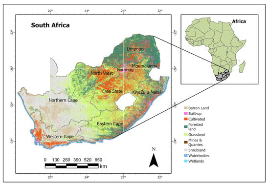
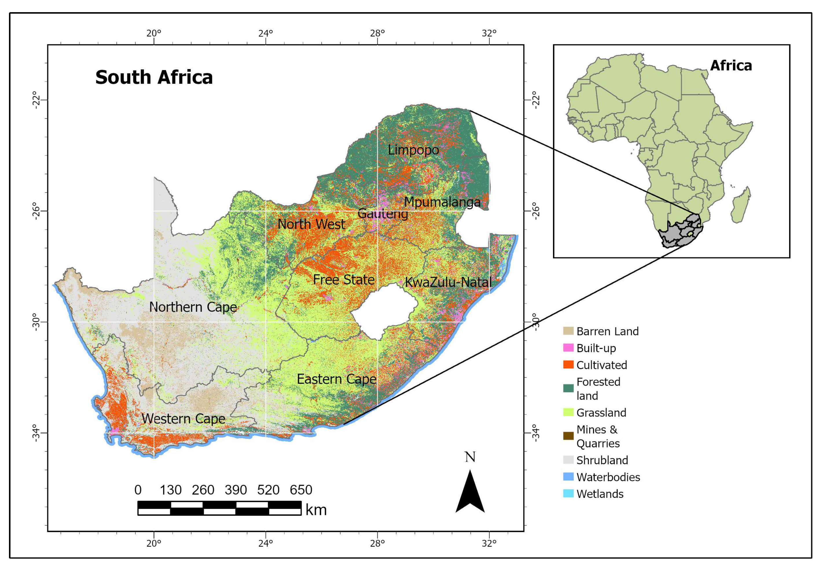
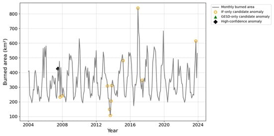
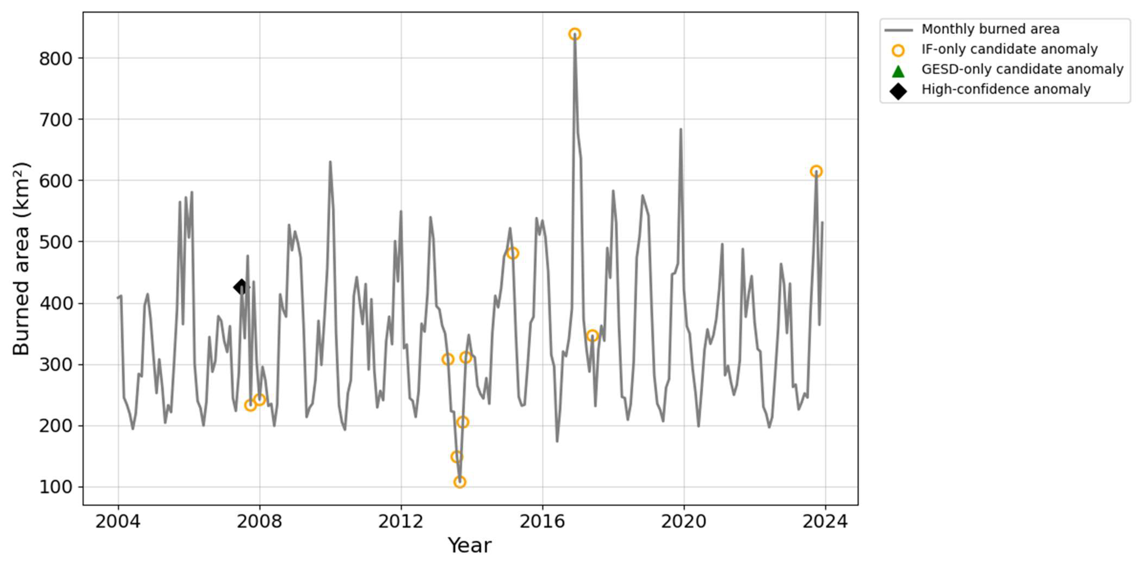
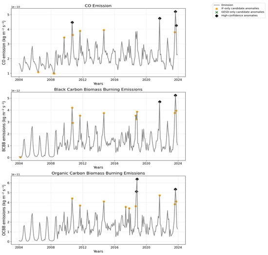
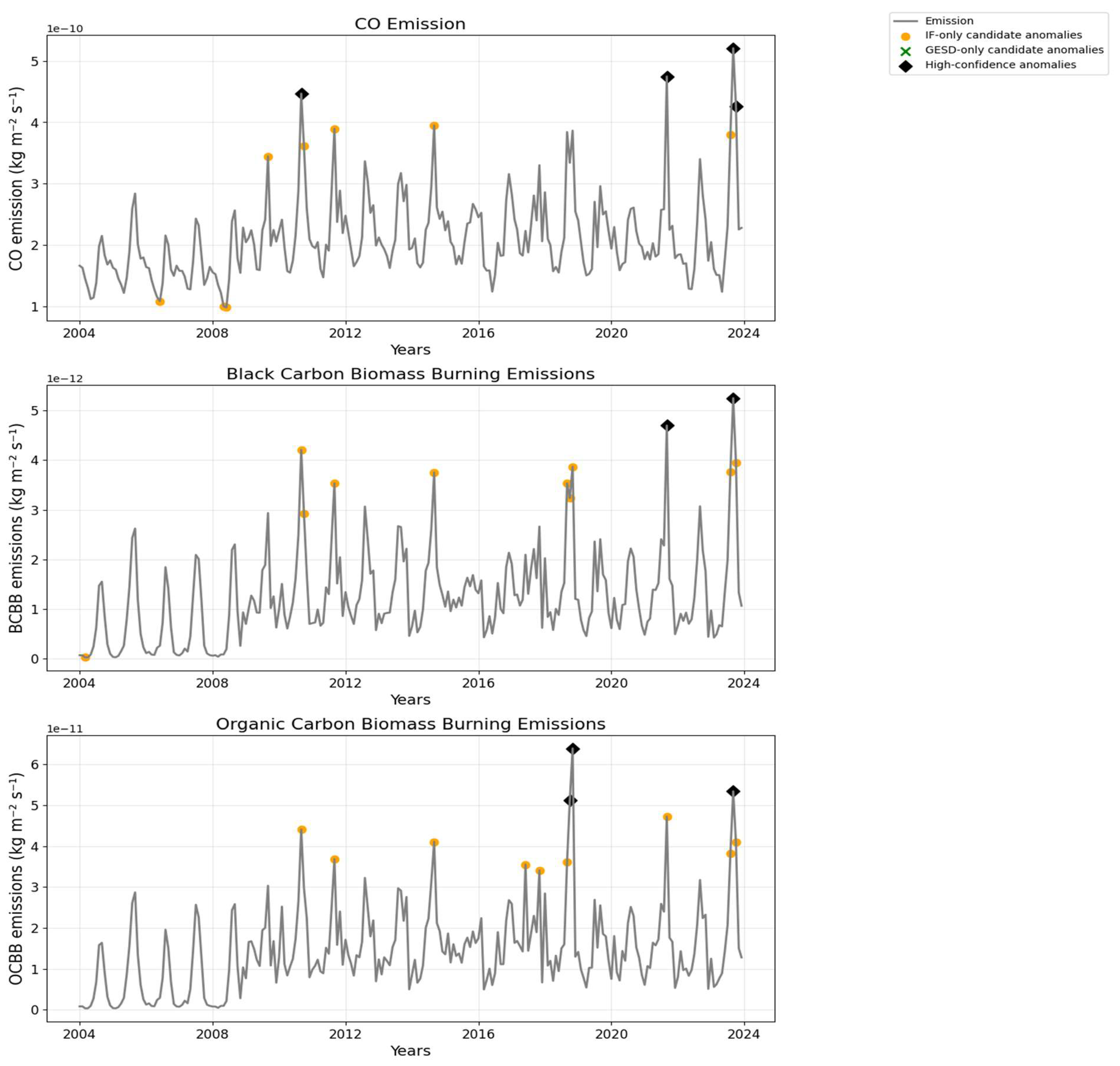
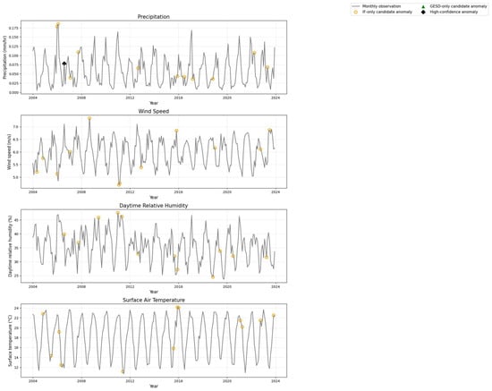
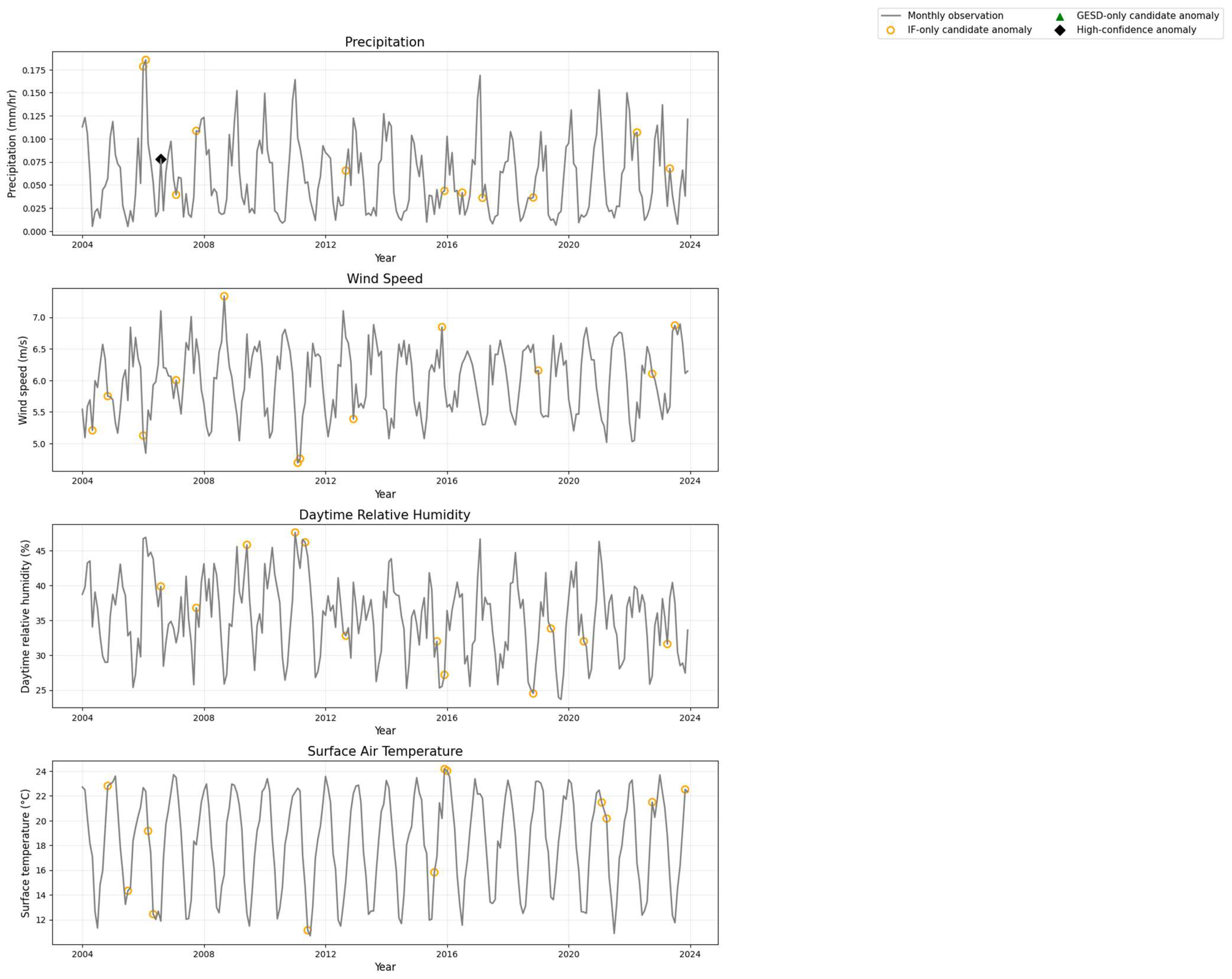
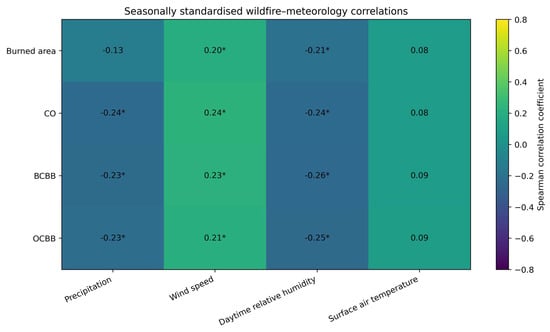
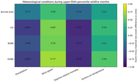
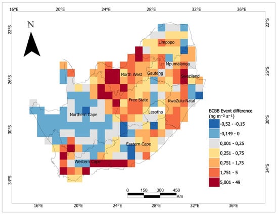
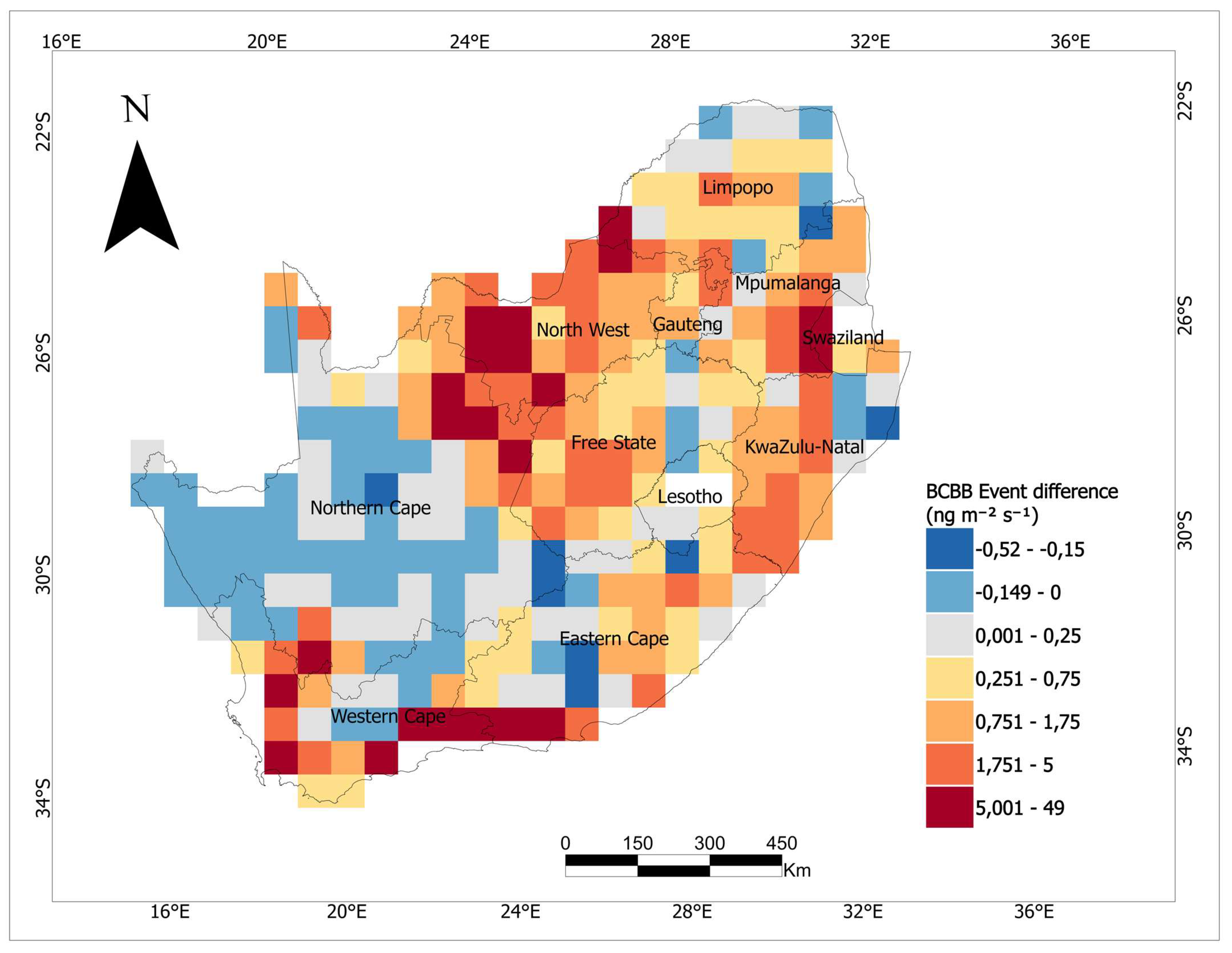
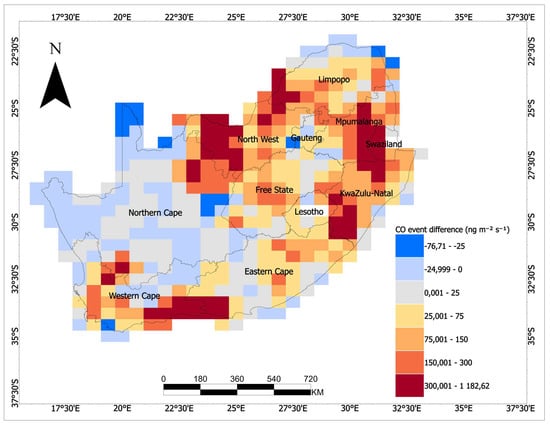
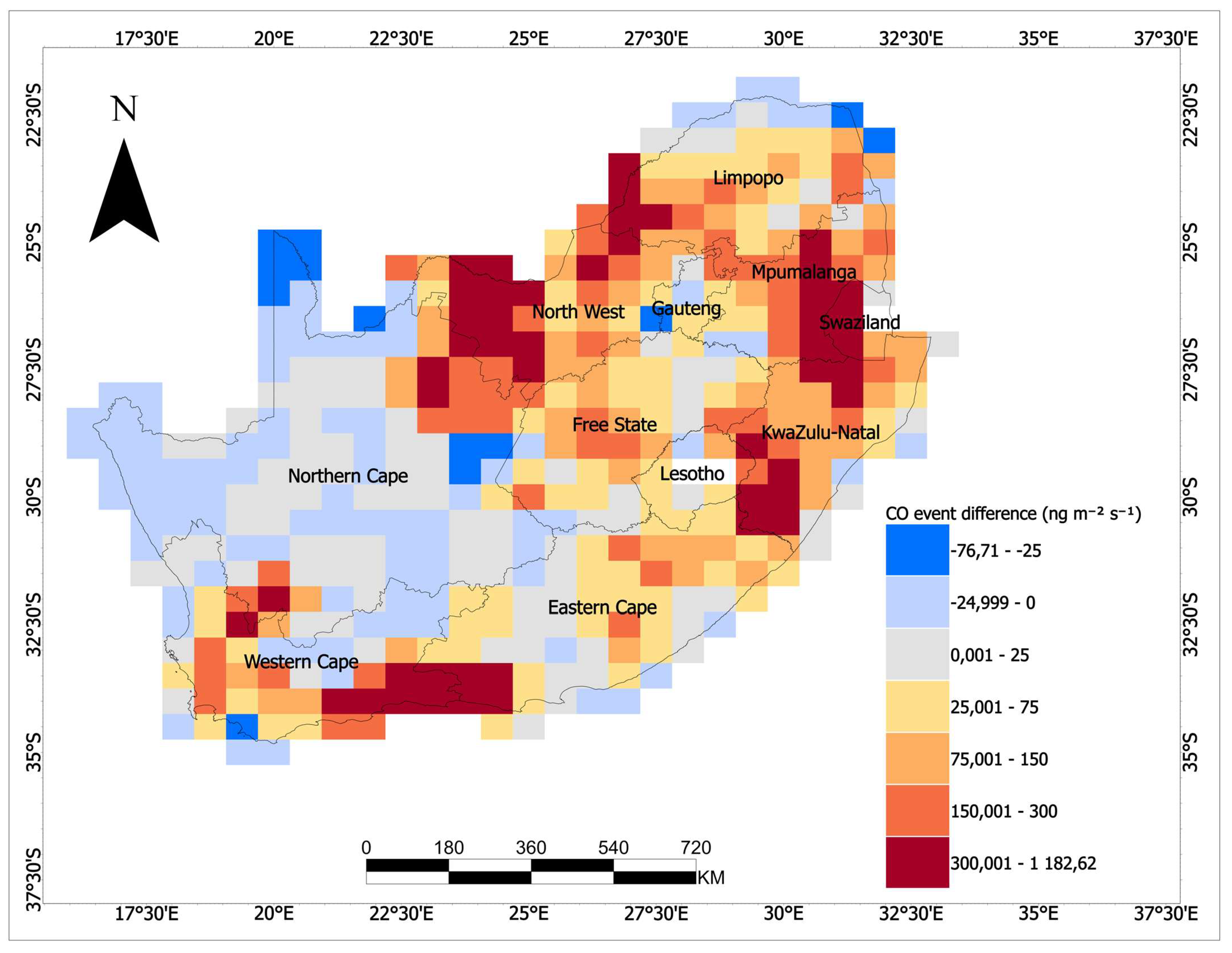
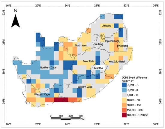
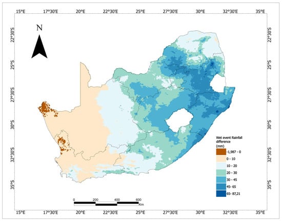
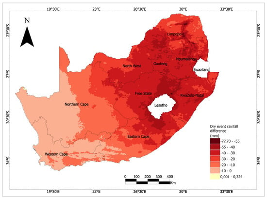
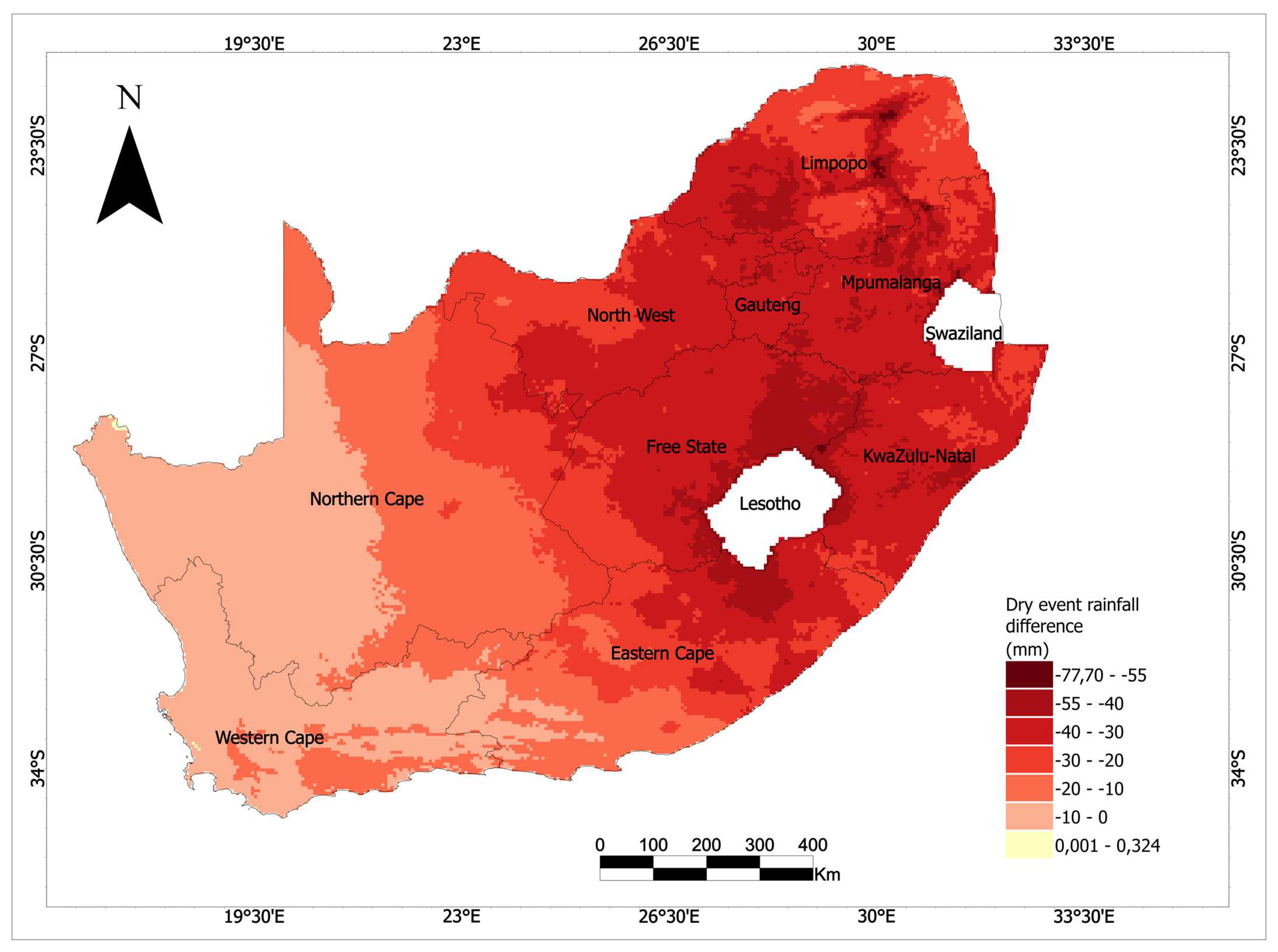
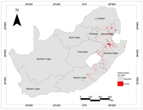
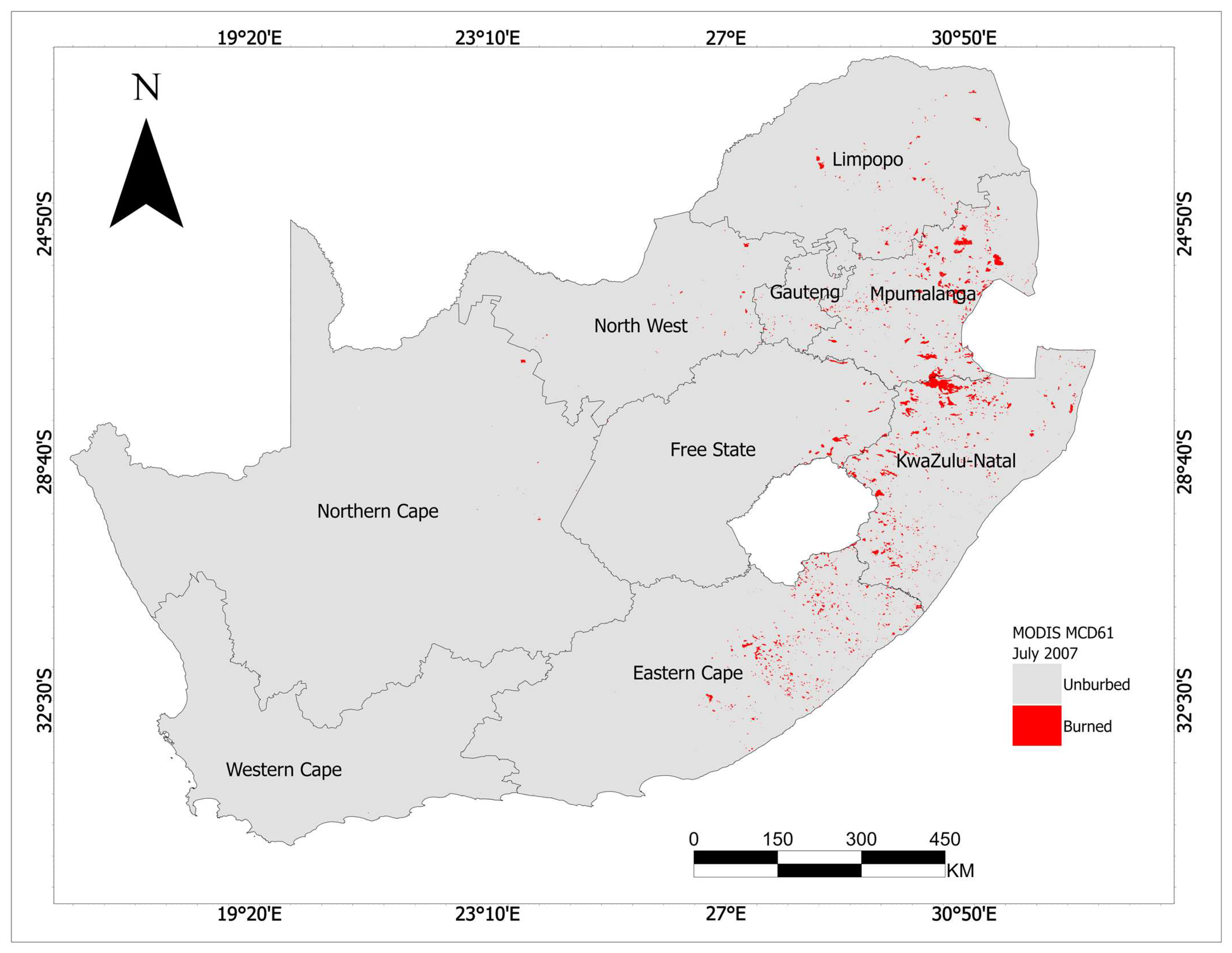
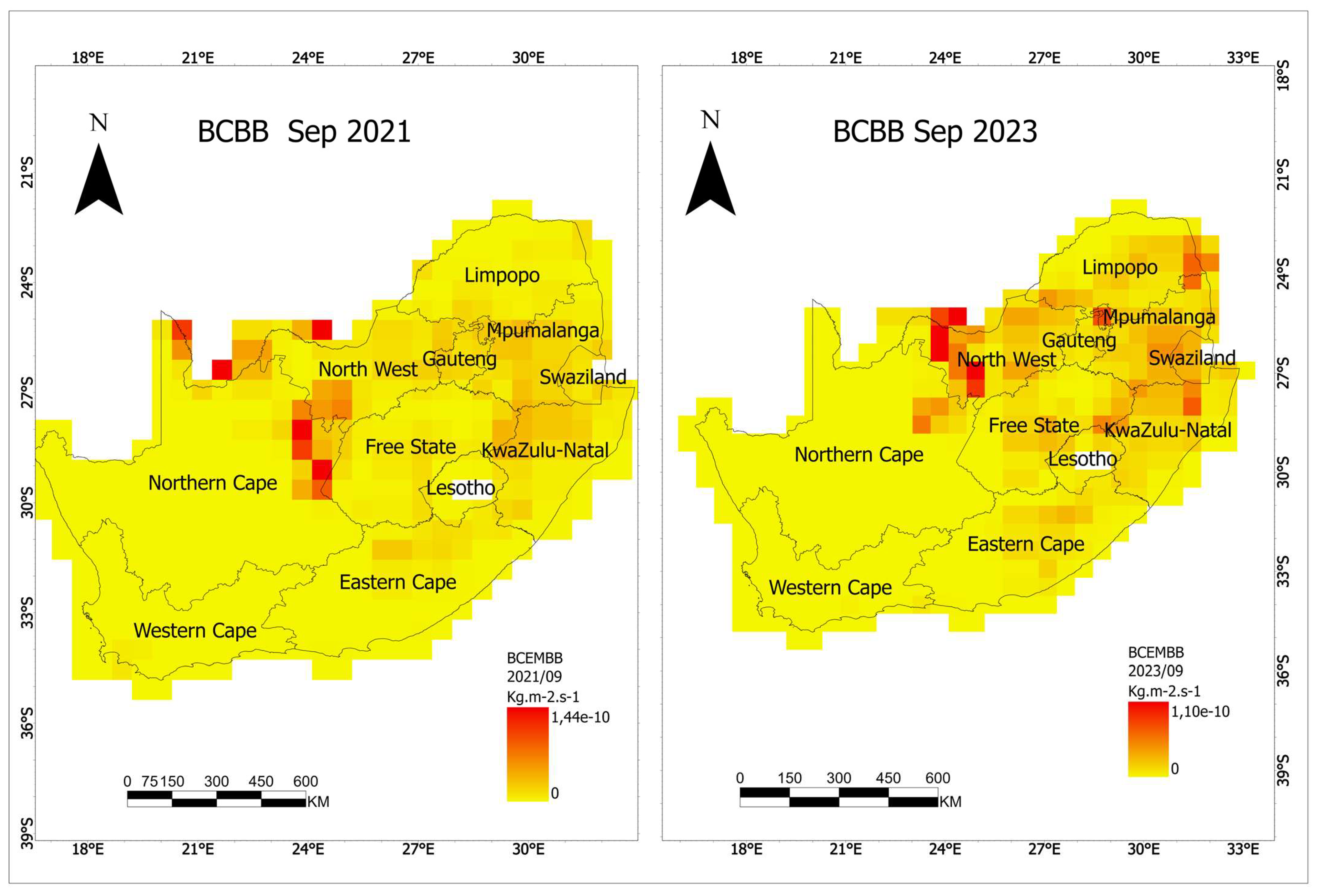
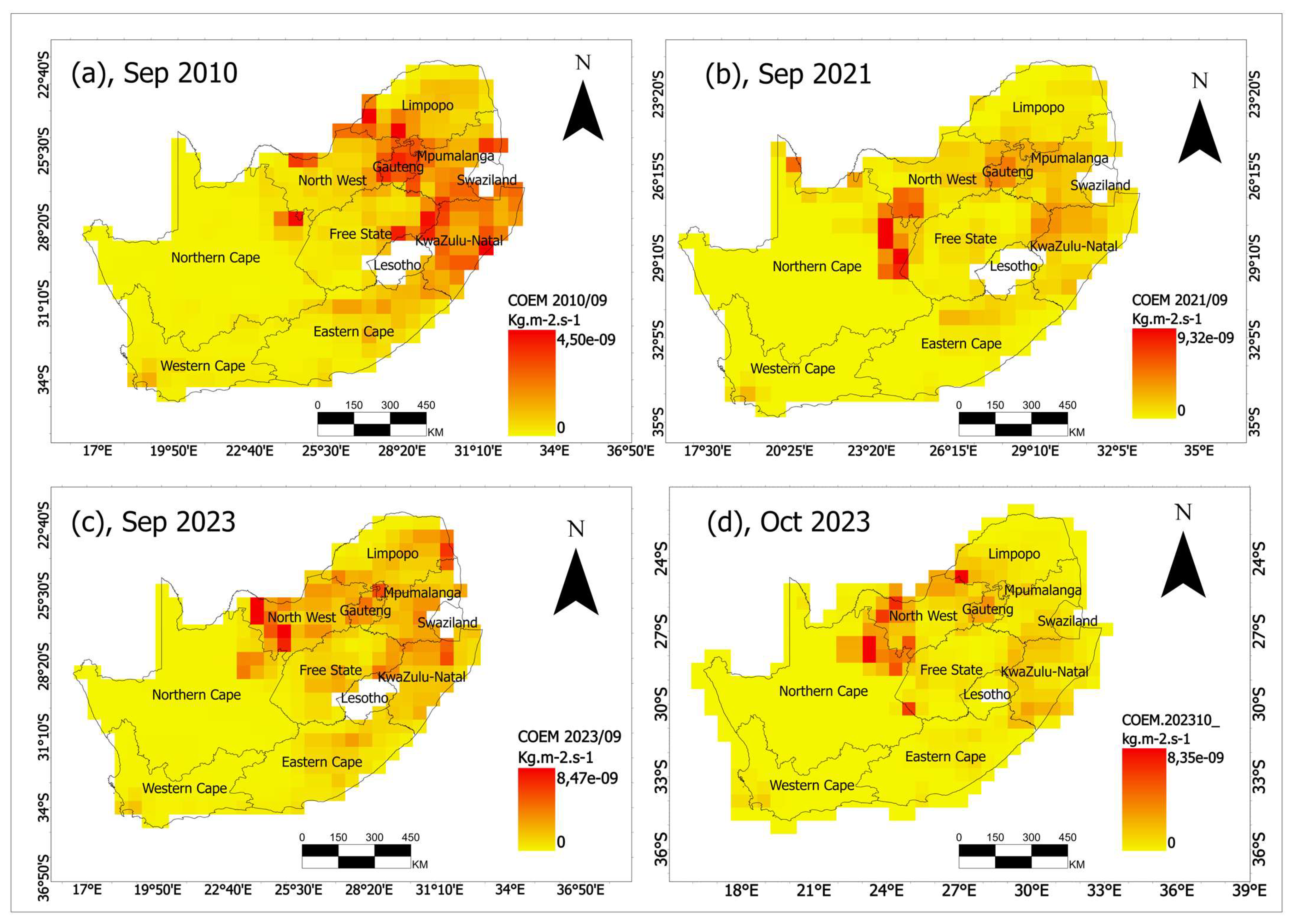
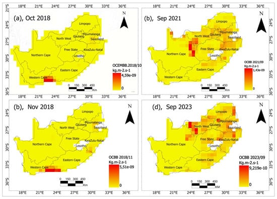
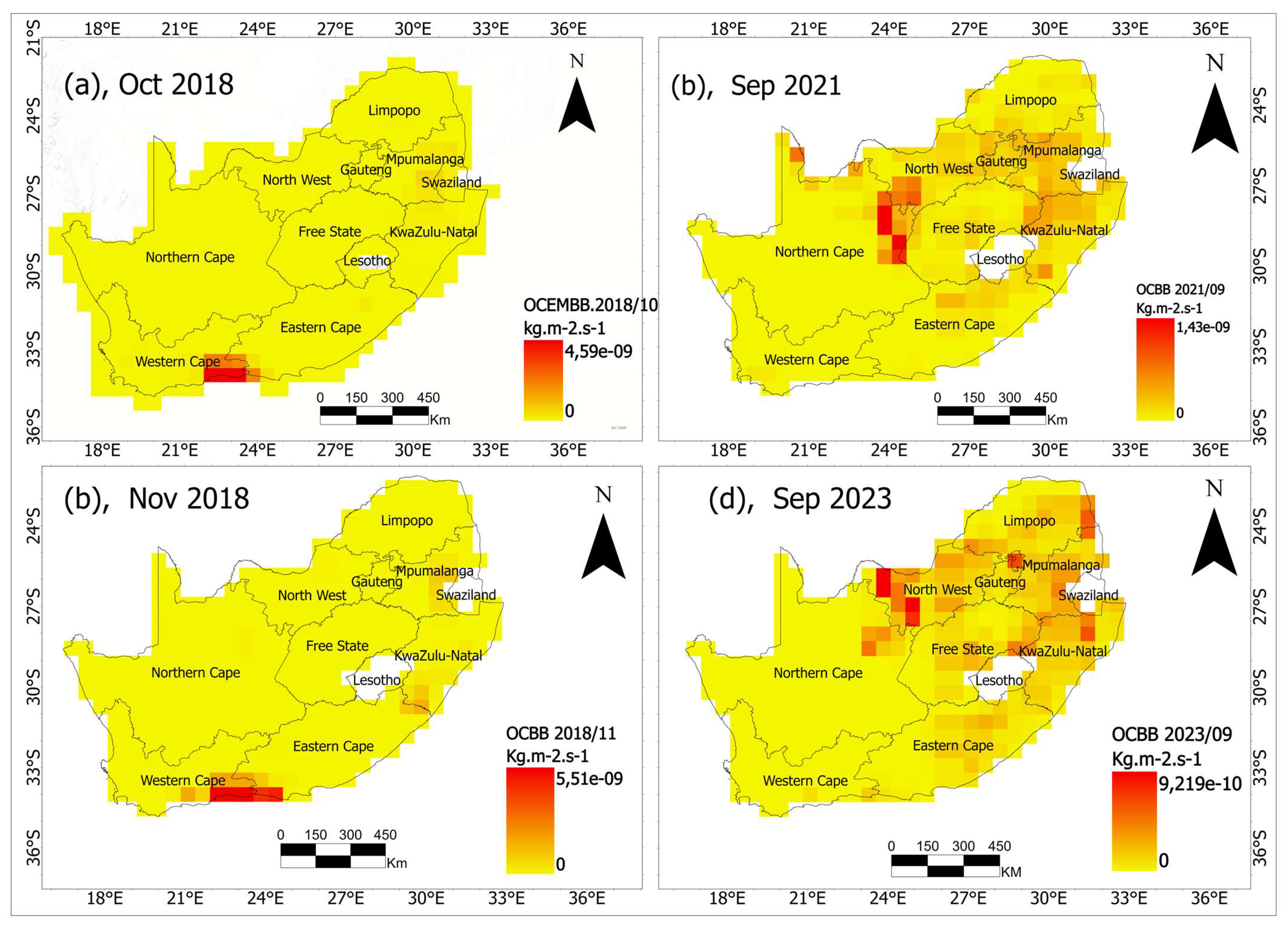
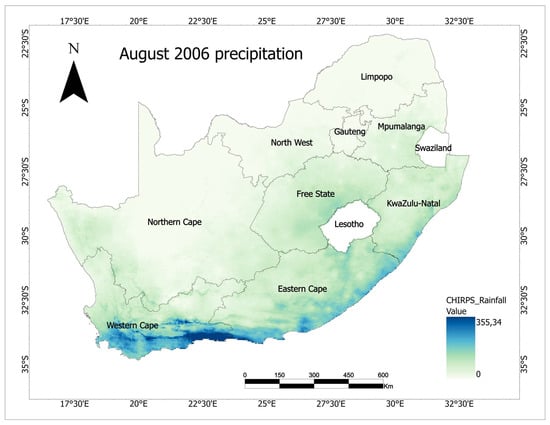
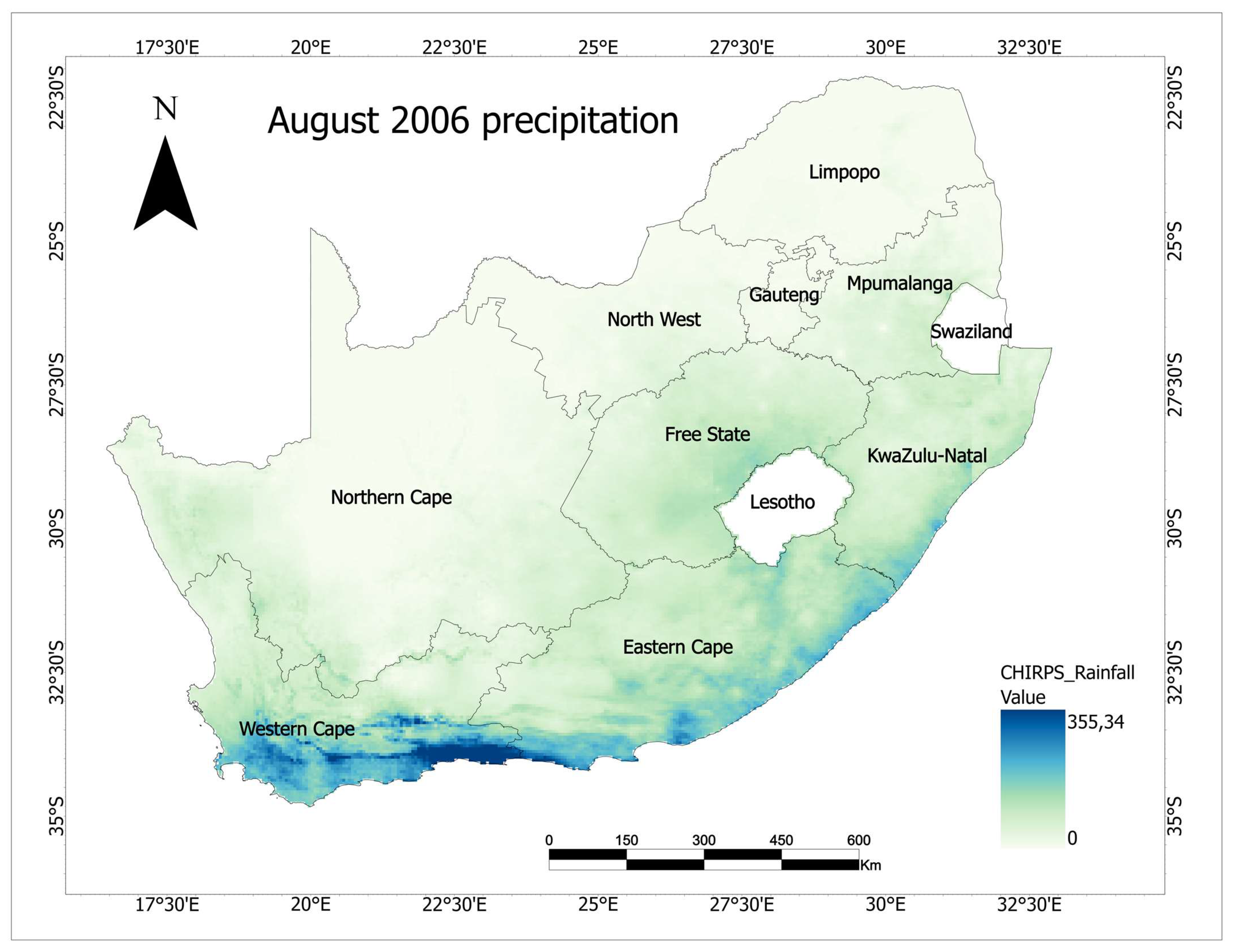

Disclaimer/Publisher’s Note: The statements, opinions and data contained in all publications are solely those of the individual author(s) and contributor(s) and not of MDPI and/or the editor(s). MDPI and/or the editor(s) disclaim responsibility for any injury to people or property resulting from any ideas, methods, instructions or products referred to in the content. |
© 2026 by the authors. Licensee MDPI, Basel, Switzerland. This article is an open access article distributed under the terms and conditions of the Creative Commons Attribution (CC BY) license.