Constraint-Aware Calibration of Power-Flow Surrogates: DG Hosting Capacity as a Downstream Application

Abstract

Power-flow surrogates reduce the cost of repeated distribution-network studies, but low regression error does not guarantee reliable feasibility decisions near technical limits. We evaluate constraint-aware calibration for a continuous-output Base–Increment multilayer perceptron trained on OpenDSS simulations of a real unbalanced medium-voltage network. The surrogate predicts electrical variables, from which voltage, loss, and conductor-loading constraints are evaluated rather than learning feasibility or hosting capacity directly. Four one-sided empirical calibration strategies are compared: output-space, uniform constraint-space, constraint-specific, and joint-vector. Configurations are selected through repeated group-aware calibration partitions and frozen before evaluation on an independent TEST partition of 3240 operating points grouped into 108 base scenarios. DG hosting capacity provides an illustrative downstream application across 72 hourly conditions, with matching OpenDSS and surrogate constraints and search procedures. High global regression accuracy coexisted with optimistic feasibility decisions near operating limits. Calibration reduced false-feasible decisions, although stronger corrections also reduced the surrogate-accepted feasible region. In the HC illustration, the uncalibrated surrogate showed the lowest hourly error but more frequent overestimation. Surrogates substantially reduced online HC computation time; offline preparation and training were excluded. These results support evaluating surrogates through both regression accuracy and decision reliability.

1. Introduction

The transition from passive distribution systems to active distribution networks is increasing the number and diversity of operating conditions that planners and operators must evaluate. Distributed photovoltaic generation, storage, flexible demand, and other distributed energy resources can alter voltage profiles, conductor utilization, losses, and reverse power flow. Hosting-capacity (HC) assessment is used to quantify how much distributed generation (DG) can be connected without violating prescribed technical criteria. The resulting value is conditional on the network model, operating state, connection point, control assumptions, and adopted limits [1,2,3]. Recent studies have examined operating-scenario assumptions and smart-inverter controls [4,5]. An experimental study in a high-altitude Ecuadorian microgrid has also examined storage-assisted smoothing of intermittent photovoltaic power as a power-quality measure [6]. HC is therefore an outcome of a constrained operating study rather than an intrinsic scalar property of a feeder.

Time-dependent HC studies are computationally demanding because load conditions must be reconstructed and power-flow equations solved repeatedly over many operating conditions and candidate generation levels. In practical distribution models, feeder-head measurements or forecasts represent aggregate demand, whereas power-flow simulation requires spatial allocation among individual customer categories and network locations. Load-allocation procedures therefore combine substation measurements with representative load patterns or historical information [7,8,9]. When embedded within a multi-hour HC search, this reconstruction adds to the computational burden of repeated power-flow solutions.

Surrogate models provide a way to reduce this burden. Machine-learning approximations of power flow have been investigated for distribution-network simulation, co-simulation, and scenario analysis [10,11,12,13]; graph-based surrogates have also been explored in broader energy-system planning [14]. More recent physics-informed neural power-flow models and safety-aware graph benchmarks incorporate physical equations or operating constraints in model development and evaluation [15,16]. Their evaluation commonly emphasizes regression metrics such as MAE, RMSE, normalized error, or the coefficient of determination. These measures characterize global numerical accuracy but not necessarily decision reliability when predicted variables are passed through technical inequalities. A prediction error that is small relative to the range of an electrical quantity may still reverse a feasibility decision near its limit.

This distinction matters in HC analysis. Learning-based approaches have been proposed to estimate HC or feasibility boundaries directly [17,18,19,20]. A polynomial-chaos Kriging surrogate has also been used to accelerate probabilistic PV hosting-capacity assessment in unbalanced networks while accounting for voltage-magnitude and voltage-unbalance constraints [21]. Other HC studies address operating uncertainty using chance-constrained voltage assessment and distributionally robust joint chance constraints [22,23]. These approaches account for uncertainty in the operating conditions, whereas the present analysis isolates the decision effects of surrogate prediction error under specified conditions. Direct HC prediction couples the learned target to a particular HC definition and may conceal which electrical condition makes an operating point inadmissible. A continuous-output power-flow surrogate offers a different compromise: voltages, losses, loading, and substation exchange remain explicit, while HC is obtained by applying constraints and a search procedure after inference. This allows the same physical outputs to be examined under alternative downstream criteria without retraining the surrogate for HC as a direct target.

The central difficulty is that surrogate residuals are not necessarily symmetric with respect to a technical boundary. If errors are directionally biased, a model with small average error can accept points that the reference power-flow model classifies as infeasible. In applications where optimistic errors have different consequences from conservative ones, symmetric regression metrics alone are insufficient. One-sided residual corrections shift predictions toward the conservative side. Their logic is related to residual-quantile and conformal-calibration methods [24,25], although coverage or risk guarantees require a specifically defined procedure and assumptions that cannot simply be transferred to shifted operating distributions [26]. Recent work has also examined conformal prediction sets for learned AC-feasibility classifiers in stochastic unit commitment [27]. Unlike direct feasibility classification, the present approach retains continuous electrical outputs and evaluates empirical calibration through downstream constraint decisions. Calibrating individual electrical outputs also does not automatically establish protection for a joint decision involving several constraints.

This study addresses that decision-level question using a continuous-output Base–Increment multilayer perceptron (MLP) trained on a detailed OpenDSS distribution-network model. Four one-sided empirical strategies are compared: output-space, uniform constraint-space, constraint-specific, and joint-vector calibration. Their settings are selected using repeated group-aware partitions of a dedicated calibration sample and frozen before independent TEST assessment. The analysis distinguishes global prediction accuracy from false-feasible rate (FFR), recall of truly feasible conditions, and distance to an OpenDSS constraint boundary.

DG hosting capacity is subsequently used as a downstream illustration, not a learning target or a comprehensive feeder-wide HC study. OpenDSS and the surrogate configurations are compared using the same DG search range, reactive-power assumption, technical constraints, and search logic. This allows HC overestimation, retained capacity, and online computation time to be examined under controlled conditions. The scope is limited to one real network, one DG connection location, and three 24 h demand trajectories; it neither claims universal HC transferability nor distribution-free feasibility guarantees.

2. Materials and Methods

2.1. Distribution Network and Operating-Condition Reconstruction

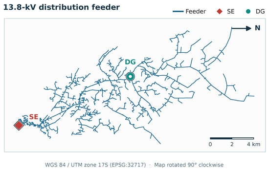
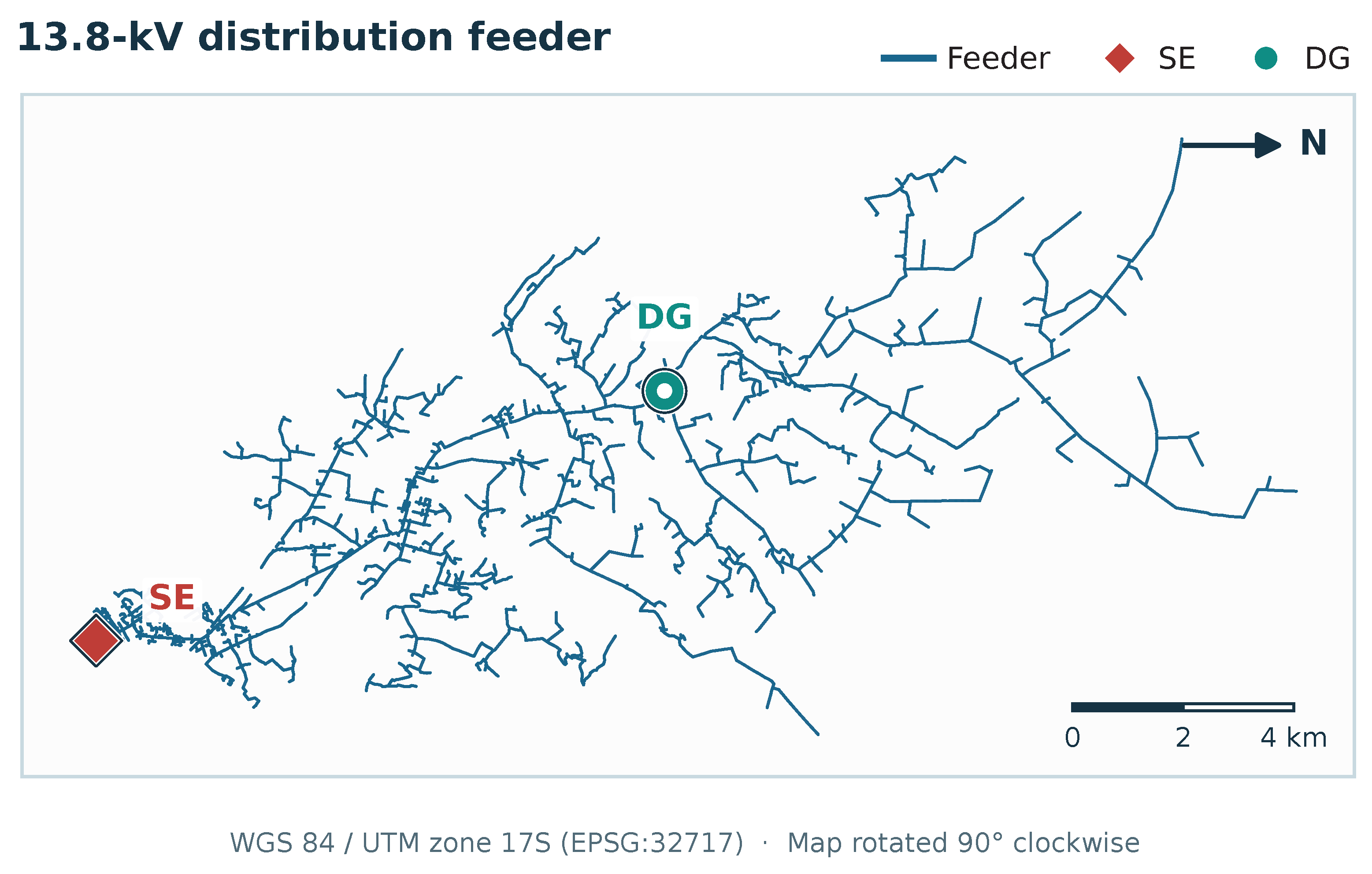
The study uses a detailed OpenDSS model of a real unbalanced radial 13.8 kV medium-voltage distribution network in Ecuador. OpenDSS is treated as the reference simulator throughout the study. The main characteristics are summarized in Table 1, while Figure 1 shows the geographical feeder representation, substation (SE), and fixed DG connection point. Geographical coordinates and medium-voltage line lengths were handled in QGIS. The map does not constitute a complete electrical single-line diagram. The OpenDSS model preserves component parameters and connectivity, but access to the model is subject to utility-data restrictions. Hourly changes in customer demand affect operating conditions, not physical feeder topology.

Table 1. Main characteristics of the studied distribution network.

Characteristic	Value
Nominal medium-voltage level	13.8 kV
Network configuration	Radial
OpenDSS buses	6391
Electrical nodes	17,410
Medium-voltage line sections	5480
Distribution transformers	910
Total transformer capacity	18.08 MVA
Modeled load objects	7280
Load categories	8
Medium-voltage network length	237.86 km
Simulation platform	OpenDSS

Figure 1. Georeferenced 13.8 kV feeder, rotated by 90° for horizontal presentation, with SE (substation) and fixed DG connection point. Scale and north direction reflect the map orientation.

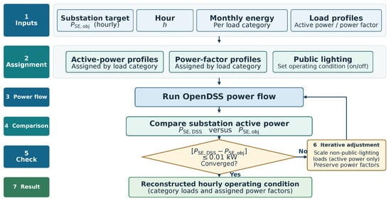
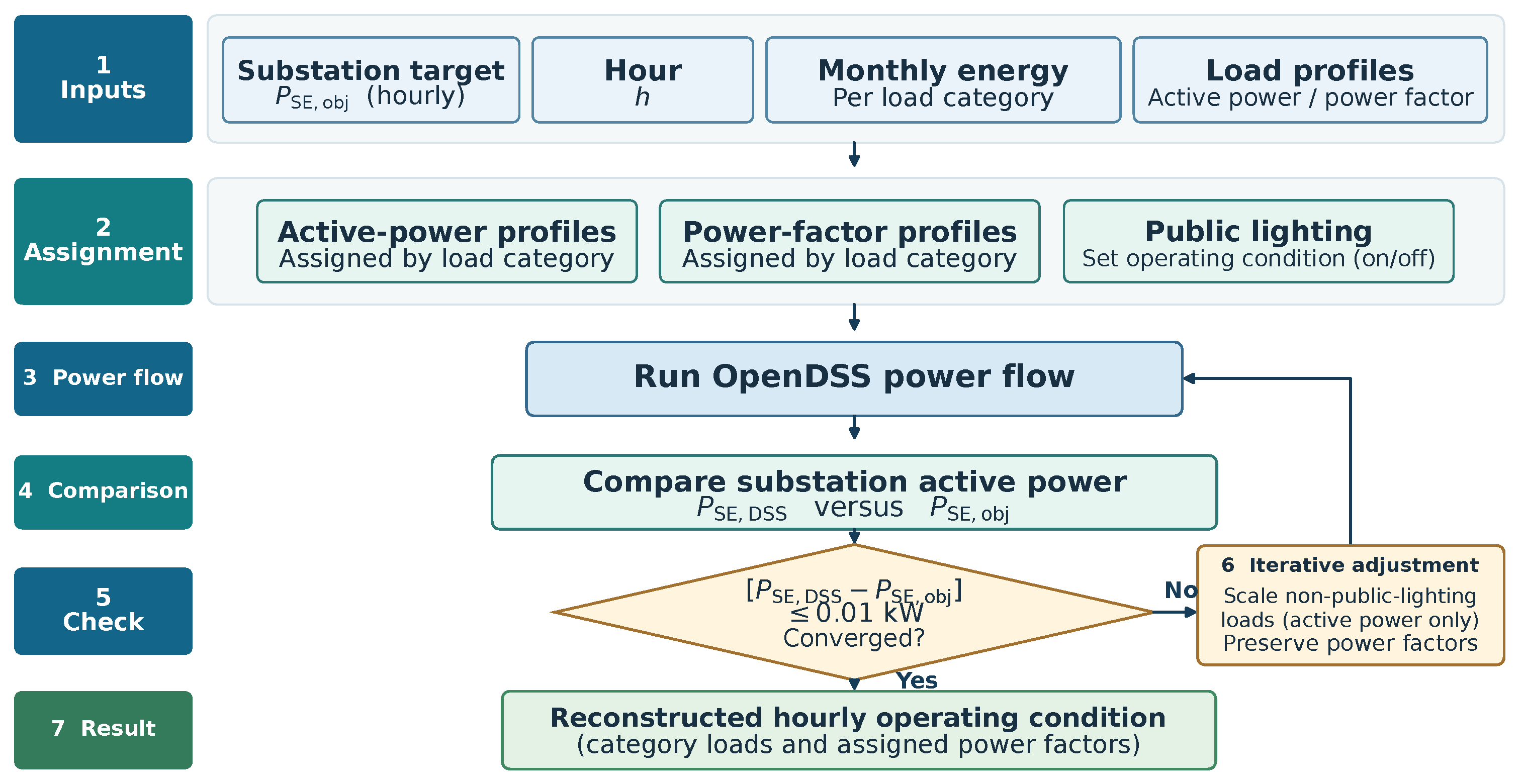
The demand representation contains eight customer-category components for each transformer: urban residential, rural residential, urban residential with electric cooking, rural residential with electric cooking, commercial, industrial, public lighting, and other uses. The 910 transformers are therefore represented by 7280 category-specific load objects. Hourly active-power and power-factor profiles are applied using previously estimated customer-category curves [28]. Public lighting follows its prescribed schedule; the other categories are then scaled until the active power calculated at the substation matches the target aggregate demand while preserving their assigned hourly power factors. Figure 2 summarizes the procedure.

Figure 2. Iterative reconstruction of each hourly OpenDSS operating condition. Category-specific active-power and power-factor profiles are applied first; non-public-lighting loads are then scaled until the substation active power matches the target condition while preserving their assigned power factors.

2.2. Dataset Generation and Base–Increment Surrogate

After reconstructing each base condition, DG operating points were generated at the fixed connection bus (Figure 1) by varying active and reactive power injection. The sampled domain was

$$0\le P_{\mathrm{DG}}\le 4500\mathrm{kW},-800\le Q_{\mathrm{DG}}\le 800\mathrm{kvar}.$$

(1)

For each base condition, 30 DG points were simulated. The sampling combined broad exploration of the $P_{\mathrm{DG}}$–$Q_{\mathrm{DG}}$ domain with additional points concentrated near electrically critical regions. The connection location was fixed; consequently, bus identity was not an input feature.

The final dataset contains 21,420 converged operating points associated with 714 unique base scenarios. Each base scenario is identified by its modeled year, date, hour, and demand percentile and comprises a substation demand target and the corresponding reconstructed customer-category load profiles. All 30 DG realizations associated with one base condition were kept in the same data partition. This grouping prevents leakage of nearly identical base operating states across training, calibration, and test subsets. Table 2 gives the final partition.

Table 2. Group-aware dataset partition used in the definitive experiment.

Subset	Base Scenarios	Operating Points	Share (%)
Training	427	12,810	59.80
Validation	72	2160	10.08
Calibration	107	3210	14.99
Independent test	108	3240	15.13
Total	714	21,420	100.00

Model-family selection was carried out only inside DEVELOPMENT, defined as training plus validation. Hyperparameters were tuned separately for the base and DG-increment prediction tasks: Ridge tested 21 logarithmically spaced penalties (${10}^{-6}$–${10}^4$); Random Forest (RF) tested 30 and 20 randomized configurations for the base and increment tasks, respectively; XGBoost tested 25 and 20; and MLP tested 12 per task. Ten repeated group-aware holdouts were then used to compare the tuned families, with 20% of DEVELOPMENT base scenarios assigned to the internal holdout in each repetition. The family with the lowest mean NRMSE was retained and refitted on complete DEVELOPMENT. Neither CALIBRATION nor TEST was used in model-family selection or final fitting.

The selected surrogate follows a Base–Increment architecture. The base MLP estimates the no-DG state, while a second MLP estimates the increments produced by $P_{\mathrm{DG}}$ and $Q_{\mathrm{DG}}$. The final state is reconstructed as

$${\widehat{\mathbf{y}}}_{\mathrm{DG}}={\widehat{\mathbf{y}}}_{\mathrm{base}}+\Delta {\widehat{\mathbf{y}}}_{\mathrm{DG}}.$$

(2)

The final output vector is

$$\widehat{\mathbf{y}}=\left[V_{\min },V_{\max },V_{\mathrm{DG},\max },P_{\mathrm{loss}},L_{\max },P_{\mathrm{SE}},Q_{\mathrm{SE}}\right],$$

(3)

where $V_{\mathrm{DG},\max }$ is retained as an auxiliary diagnostic output, while the formal HC constraints use the system-wide $V_{\min }$ and $V_{\max }$ values. The base model has 22 inputs and six outputs; the DG-increment model has 24 inputs and seven outputs (full definitions in Appendix A). The six base outputs are minimum and maximum system voltages, the voltage diagnostic at the future DG bus, losses, maximum loading, and substation reactive power. Baseline substation active power $P_{\mathrm{SE}}^{\mathrm{base}}$ is a measured input, not a predicted base output. Consequently, its DG-state value is $P_{\mathrm{SE}}^{\mathrm{base}}+{\widehat{\Delta P}}_{\mathrm{SE}}$, while the other six DG-state outputs add a predicted increment to the corresponding predicted baseline. Predicted baseline voltages, losses, and loading are the reference values used when evaluating the base-relative surrogate constraints, including in the direct-MLP diagnostic comparison. Numerical inputs and outputs are standardized using scaling parameters estimated from the development data.

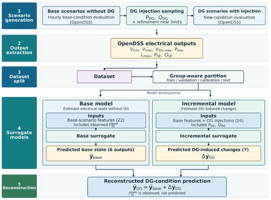
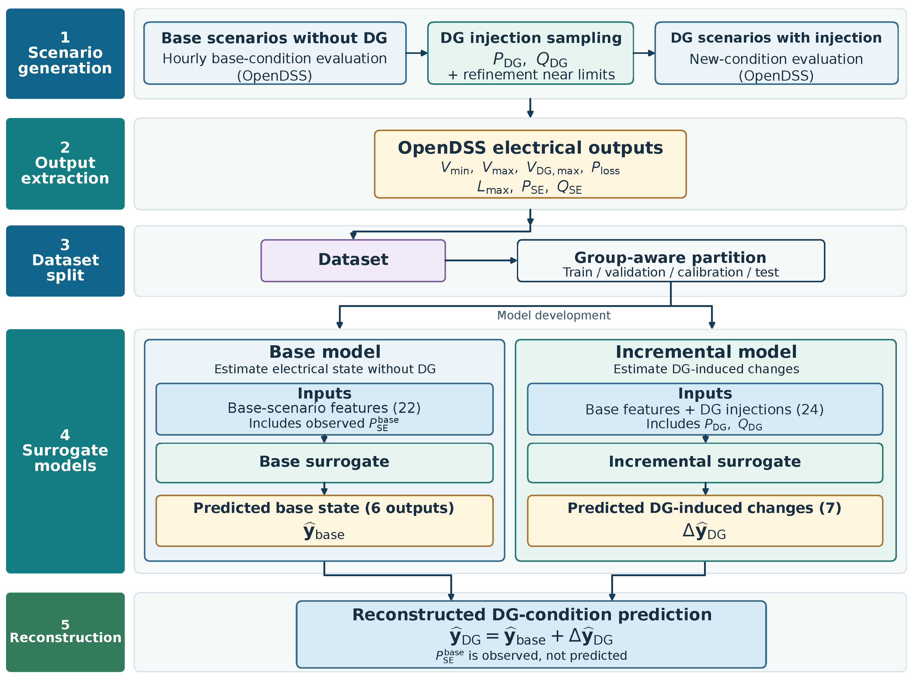
The Base–Increment formulation supplies the same learning targets to all four regression families, separating between-scenario baseline variation from within-scenario DG responses (Figure 3). Baseline outputs are invariant across the 30 DG realizations within each scenario, even though DG sampling may correlate with baseline characteristics across scenarios. This interpretable comparison structure does not presume superiority over direct regression.

Figure 3. Dataset-generation workflow and Base–Increment surrogate formulation. OpenDSS evaluates the reconstructed base condition and the sampled DG operating points; the resulting data are partitioned before the base-state and DG-increment surrogates are trained and combined. Values in parentheses represent model input/output dimensions.

No exact identity $\Delta {\widehat{\mathbf{y}}}_{\mathrm{DG}}(0,0)=\mathbf{0}$ was enforced. We therefore evaluated the frozen incremental MLP at zero injection for the 108 independent TEST base scenarios; its component-wise errors relative to zero are reported in Appendix B.

2.3. Technical Constraints and Error Orientation

The surrogate is not trained to predict feasibility directly. Instead, feasibility is derived from four explicit constraint functions evaluated using its continuous electrical outputs. The calibration strategies act on those outputs or the corresponding constraint estimates before determining admissibility. Ecuadorian Regulation ARCONEL-009/2024 (codified, as amended by Resolution ARCONEL-030/2025) specifies an allowable medium-voltage variation of $\pm 6\%$ from nominal voltage [29], corresponding to 0.94–1.06 p.u. These thresholds inform the voltage criteria below, but the baseline-adapted lower bound and the scenario-level checks are study-specific rather than a regulatory compliance assessment. For each operating point,

$$\begin{array}{cc}\hfill g_{V_{\min }}& =\min \left(V_{\min }^{\mathrm{base}},0.94\right)-V_{\min }^{\mathrm{DG}},\hfill \end{array}$$

(4)

$$\begin{array}{cc}\hfill g_{V_{\max }}& =V_{\max }^{\mathrm{DG}}-1.06,\hfill \end{array}$$

(5)

$$\begin{array}{cc}\hfill g_{\mathrm{Loss}}& =P_{\mathrm{loss}}^{\mathrm{DG}}-P_{\mathrm{loss}}^{\mathrm{base}},\hfill \end{array}$$

(6)

$$\begin{array}{cc}\hfill g_{\mathrm{Loading}}& =L_{\max }^{\mathrm{DG}}-\min \left(L_{\max }^{\mathrm{base}},100\right).\hfill \end{array}$$

(7)

An operating point is admissible when

$$g_j\le 0\forall j.$$

(8)

The minimum-voltage criterion uses 0.94 p.u. unless the baseline is already below it; in that case, DG must not worsen the system-wide minimum. This condition does not protect every individual node. Maximum voltage has an absolute 1.06 p.u. limit. Loading must not exceed its baseline maximum when that maximum is below 100%, or 100% otherwise; losses must not increase from the no-DG state. The loss and baseline-relative loading criteria are conservative choices for this study, not universal grid-code requirements. This asymmetric voltage rule admits a baseline-undervoltage state if DG does not worsen its minimum but never relaxes the 1.06 p.u. upper limit; HC is consequently conditional on this definition. All four functions share the sign convention $g_j>0$ for violation and $g_j\le 0$ for feasibility, but their values have different units.

For constraint-space calibration, prediction error is oriented so that positive error represents an optimistic surrogate estimate:

$$e_{g_j}=g_j^{\mathrm{DSS}}-{\widehat{g}}_j.$$

(9)

For any calibration percentile p, the one-sided empirical margin is

$$\delta \left(p\right)=\max \left[0,Q_p\left(e\right)\right],$$

(10)

where $Q_p$ is evaluated using the empirical higher-order statistic. Constraint-space calibration is then applied as

$${\widehat{g}}_j^{\mathrm{cal}}={\widehat{g}}_j+{\delta }_{g_j}\left(p\right).$$

(11)

Because every constraint is defined with violation sign $g_j>0$, adding ${\delta }_j\ge 0$ tightens acceptance (${\widehat{g}}_j\le -{\delta }_j$), including for minimum voltage, where a larger $g_{V_{\min }}$ denotes a lower DG-state voltage.

Output-space calibration uses an analogous one-sided orientation. For $V_{\max }$, active losses, and loading, $e_y=y_{\mathrm{DSS}}-\widehat{y}$, whereas for $V_{\min }$, $e_y=\widehat{y}-y_{\mathrm{DSS}}$. The calibrated outputs are therefore increased for $V_{\max }$, losses, and loading and decreased for $V_{\min }$. These corrections are applied only to the reconstructed DG-state predictions. The predicted baseline quantities remain uncorrected when evaluating baseline-dependent constraints.

A utility permitting an increase in losses would obtain a different HC and would need to reassess calibration under its own criteria.

2.4. Repeated Grouped Calibration and Frozen Strategies

Calibration uses only the CALIBRATION partition, which contains 107 base scenarios and 3210 operating points. Twenty repeated CAL-FIT/CAL-VAL partitions are created by grouping on the base-scenario identifier, with 70% of base scenarios used to estimate candidate one-sided margins and 30% used to evaluate the resulting decisions. The same grouped partitions are reused by all four calibration strategies; no TEST cases enter this procedure. After selecting the configurations from these repeated partitions, the margins are re-estimated using the complete CALIBRATION partition and frozen before TEST evaluation.

Candidate percentiles are $50,52.5,55,\dots ,95,97.5,99,$ and $99.5\%$. Output-space and Uniform each select one percentile for their respective margin definitions. For both, FFR and recall are averaged over the 20 CAL-VAL splits: candidates with mean $\mathrm{FFR}\le 1\%$ are ranked first by higher mean recall, then by lower FFR, and finally by a lower percentile. If no candidate meets the FFR threshold, the one with the lowest mean FFR is used. Constraint-specific selects each constraint’s percentile within each split by zero false-feasible cases, recall, true-feasible count, and then lower percentile; the most frequent selection across splits is frozen, with the lower level breaking a frequency tie.

Joint-vector allows each of four constraints to remain raw (uncorrected) or receive a candidate percentile. The 16 distinct vectors proposed across individual splits are cross-evaluated on all 20 splits. Among vectors with mean $\mathrm{FFR}\le 1\%$, the ranking uses mean recall, mean FFR, frequency of meeting the FFR target, summed percentile levels, and number of corrected components. “Less aggressive” refers to a lower percentile within one margin definition, not a smaller numerical margin across quantities with different units. These criteria are empirical: CAL-VAL FFR of zero does not imply zero FFR on TEST or a formal coverage guarantee.

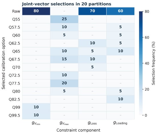
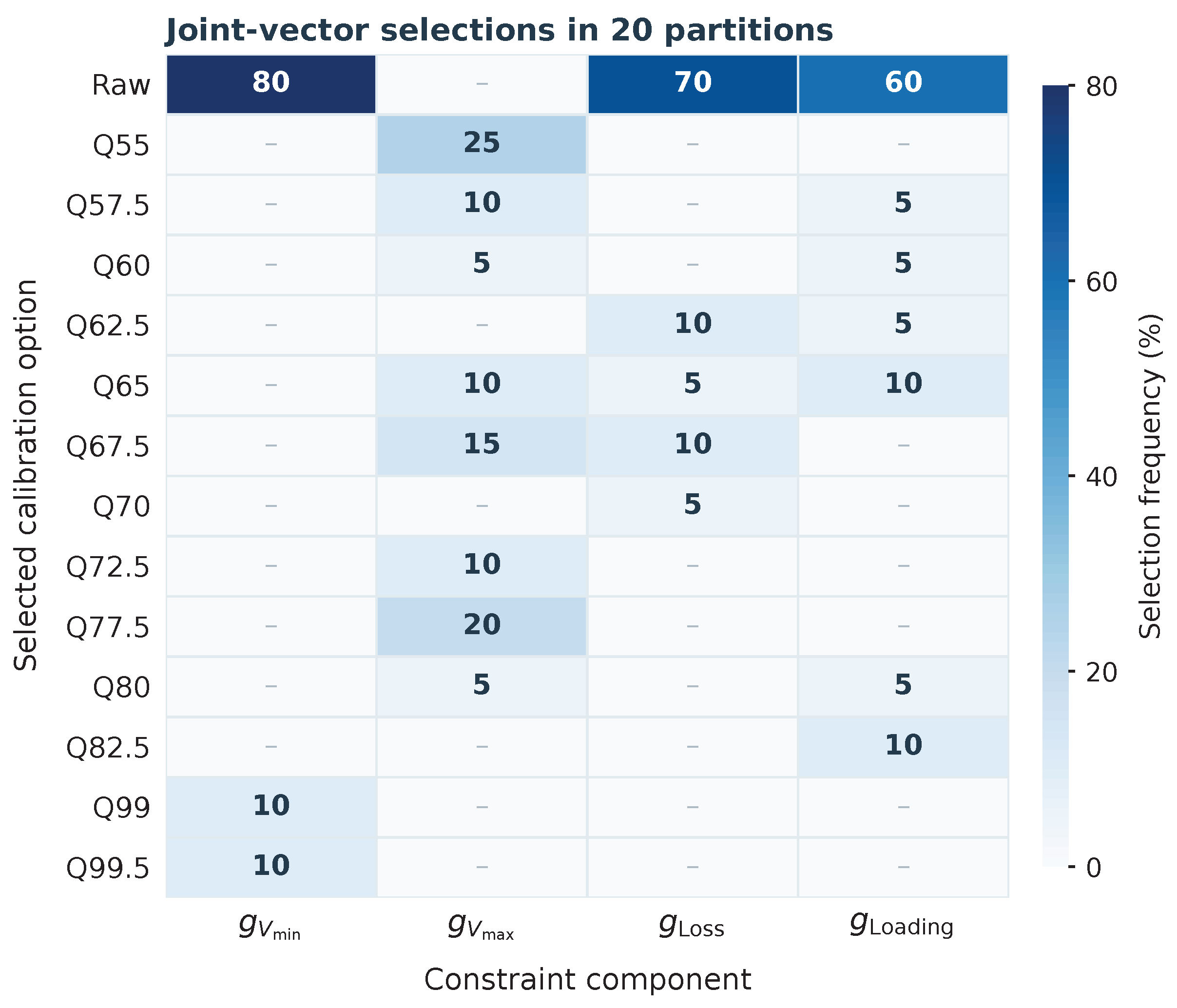
After selecting the calibration structures, the final margins are estimated once from the entire CALIBRATION partition and frozen. The final frozen configurations are shown in Table 3, and the numerical margins are reported in Appendix F. TEST is evaluated only after this freeze. Figure 4 shows that joint-vector choices vary across constraints: the minimum-voltage component is most frequently left uncorrected, while the maximum-voltage component spans several quantiles. These are empirical selection frequencies, not probabilities of constraint satisfaction.

Table 3. Frozen calibration configurations selected before opening TEST. The order of constraint-vector entries is $g_{V_{\min }}$, $g_{V_{\max }}$, $g_{\mathrm{Loss}}$, and $g_{\mathrm{Loading}}$.

Strategy	Configuration	Mean FFR (%)	Mean Recall (%)	FFR Std. (p.p.)	Recall Std. (p.p.)
Output-space	Q57.5	0.8386	91.1232	0.4021	1.9066
Uniform constraint	Q70	0.9710	93.3800	0.4462	1.5613
Constraint-specific	Q97.5|Q97.5|Q97.5|Q80	0.0000	85.5727	0.0000	2.2745
Joint-vector	Raw|Q77.5|Raw|Raw	0.9795	93.6785	0.4592	1.5564

Figure 4. Selection-frequency structure of the joint-vector calibration across the repeated grouped CAL-FIT/CAL-VAL partitions.

2.5. Independent Feasibility Assessment

The definitive independent TEST partition contains 3240 operating points from 108 base scenarios. Feasibility is recomputed from the formal constraints in Equation (8); a legacy feasibility flag stored during dataset generation is not used to calculate the reported metrics because it does not exactly reproduce the final formal constraint definition.

Each surrogate decision is classified as true feasible (TP), false feasible (FP), true infeasible (TN), or false infeasible (FN). The principal decision metrics are

$$\mathrm{Recall}={\displaystyle \frac{TP}{TP+FN}},$$

(12)

and

$$\mathrm{FFR}={\displaystyle \frac{FP}{TP+FP}}.$$

(13)

FFR is the fraction of surrogate-accepted operating points classified as infeasible by the OpenDSS reference; recall is the fraction of OpenDSS-feasible points retained. Thus, FFR is an empirical false-discovery proportion among accepted points, not the conventional false-positive rate $FP/(FP+TN)$, whose denominator is all reference-infeasible points. The accepted-set denominator is useful when screening candidate operating points, but it does not establish a probability of failure under field operating conditions.

Boundary proximity is described by the minimum normalized distance to a violated OpenDSS constraint. Because a minimum distance does not measure the worst violation across simultaneous failures, we also report $d_{\max }={\max }_j\{\max (0,g_j^{\mathrm{DSS}})/s_j\}$, where each $s_j>0$ is a constraint-specific reference scale, expressed in the same units as $g_j$, estimated from CALIBRATION and held fixed for TEST. Both are descriptive, dimensionless diagnostics; physical-unit HC violations are reported in the hosting-capacity results.

2.6. Hosting-Capacity Assessment

HC is used as a downstream, illustrative application of the continuous-output surrogate. To isolate the response to active-power injection at the fixed DG bus, every HC search assumes unity power factor and therefore fixes reactive injection at

$$Q_{\mathrm{DG}}=0.$$

(14)

Although the surrogate was trained over $-800$ to 800 kvar, Volt–Var control and inverter limits are outside this illustrative HC experiment and could change the HC boundary. The hourly HC for evaluator m is

$${\mathrm{HC}}_h^{\left(m\right)}=\max \left\{P_{\mathrm{DG}}:g_j^{\left(m\right)}(h,P_{\mathrm{DG}},0)\le 0\forall j\right\}.$$

(15)

The validated search domain is restricted to $0\le P_{\mathrm{DG}}\le 4500$ kW, matching the active-power domain used to construct the surrogate dataset.

OpenDSS and every surrogate use the same coarse-to-fine search: a global 100 kW scan across 0–4500 kW and then 10 kW refinement within $\pm 100$ kW and 1 kW refinement within $\pm 10$ kW of the largest feasible candidate. Monotonicity is not assumed; if 4500 kW is feasible, HC is right-censored.

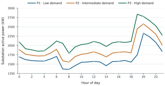
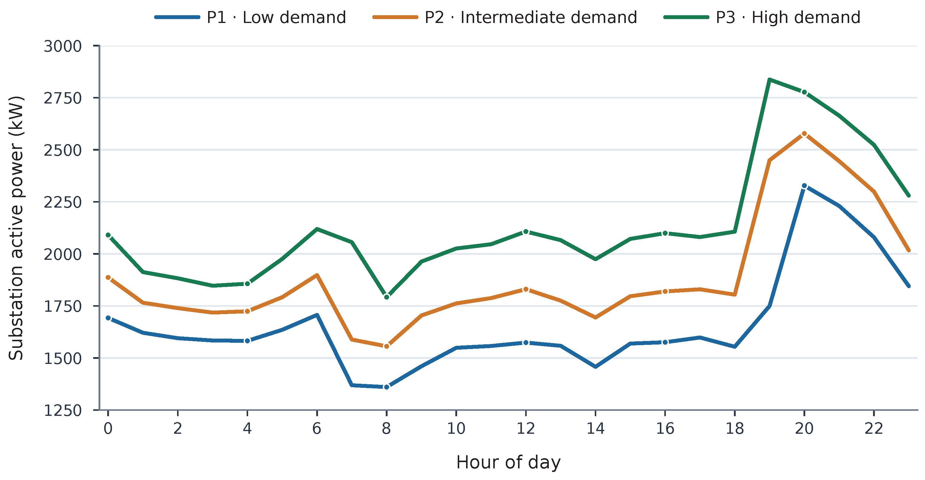
Three 24 h load trajectories for 7 September 2026 represent P5, P50, and P95 demand assumptions (P1–P3) for the same date, rather than three independent days. They were selected before HC calculation; the 72 hourly base scenarios overlap with DEVELOPMENT (49), CALIBRATION (11), and TEST (12), so the HC case study is not an additional independent test sample. Their characteristics are reported in Table 4, and Figure 5 shows their hourly demand trajectories. Hourly HC is the largest feasible DG injection detected for one hour by the specified search. A fixed DG rating must instead satisfy all 24 hourly constraint sets simultaneously:

$${\mathrm{HC}}_{24\mathrm{h},\mathrm{ideal}}^{\left(m\right)}=\max \{P\in \mathcal{P}:g_j^{\left(m\right)}(h,P,0)\le 0\forall h,j\},$$

(16)

Here, $\mathcal{P}=[0,4500]$ kW defines the conceptual continuous domain. The reported numerical estimate is ${\widehat{\mathrm{HC}}}_{24\mathrm{h}}^{\left(m\right)}=U_m$, where $U_m={\min }_h{\widehat{\mathrm{HC}}}_h^{\left(m\right)}$ comes from the hourly coarse-to-fine searches and is then checked against all four constraints in all 24 h. All 18 profile/evaluator candidates passed this joint check, preserving the reported estimates. Thus, feasibility is verified for each evaluator, but continuous global optimality is not established by these finite searches.

Table 4. Three 24 h demand trajectories (P5/P50/P95 on 7 September 2026) used for the downstream HC assessment.

Profile	Demand Level	Mean ${\mathit{P}}_{\mathbf{SE}}$ (kW)	Min–Max ${\mathit{P}}_{\mathbf{SE}}$ (kW)	24 h Energy (kWh)
P1	Low	1659.832	1360.471–2327.817	39,835.971
P2	Intermediate	1886.024	1556.222–2578.136	45,264.566
P3	High	2131.627	1792.342–2837.398	51,159.059

Figure 5. Low-, intermediate-, and high-demand scenarios (P5/P50/P95) for 7 September 2026.

For the 72 hourly conditions, surrogate HC error is defined as

$$e_h^{\left(m\right)}={\mathrm{HC}}_h^{\left(m\right)}-{\mathrm{HC}}_h^{\mathrm{DSS}},$$

(17)

so that positive error indicates HC overestimation. Agreement is summarized using MAE, RMSE, MAPE, and mean bias. A case is counted as an overestimation when $e_h>0.5$ kW, consistent with the final 1 kW search resolution. Mean retained HC is calculated as

$${\mathrm{HC}}_{\mathrm{ret}}^{\left(m\right)}={\displaystyle \frac{100}{H}}{\displaystyle \sum _{h=1}^H}{\displaystyle \frac{\min \left({\mathrm{HC}}_h^{\left(m\right)},{\mathrm{HC}}_h^{\mathrm{DSS}}\right)}{{\mathrm{HC}}_h^{\mathrm{DSS}}}},$$

(18)

which prevents an optimistic overestimate from being interpreted as more than 100% retained capacity.

Equation (18) summarizes average hourly retained HC (72 conditions); Equation (16) defines the ideal joint 24 h problem, for which a feasible numerical candidate is reported. A high hourly average need not imply a high jointly admissible capacity. No reference HC was right-censored.

2.7. Computational-Time Assessment

Computational time is separated into three quantities: hourly OpenDSS load reconstruction, OpenDSS HC search, and surrogate HC search. For each hourly condition, the OpenDSS base load is reconstructed only once; all subsequent HC candidates use the same reconstructed load distribution and vary only DG injection. TensorFlow warm-up and OpenDSS compilation are excluded from the reported online times. Two speedups are reported:

$$S_{\mathrm{search}}={\displaystyle \frac{t_{\mathrm{HC},\mathrm{DSS}}}{t_{\mathrm{HC},\mathrm{surr}}}},S_{\mathrm{workflow}}={\displaystyle \frac{t_{\mathrm{recon},\mathrm{DSS}}+t_{\mathrm{HC},\mathrm{DSS}}}{t_{\mathrm{HC},\mathrm{surr}}}}.$$

(19)

The timing measurements were obtained in Google Colab on an Intel Xeon CPU at 2.20 GHz, with two available logical processors and 12.67 GiB of RAM, without GPU acceleration. OpenDSS and surrogate HC searches were executed sequentially within the same benchmarking procedure, using time.perf_counter() to measure execution times. Since the measurements correspond to single runs, the speedup factors are specific to this computing environment and should not be interpreted as hardware-independent performance estimates.

Training and dataset-generation costs are offline and are not included in these online-assessment speedups.

3. Results

3.1. Surrogate Selection and Independent Prediction Accuracy

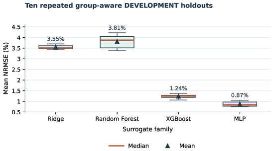
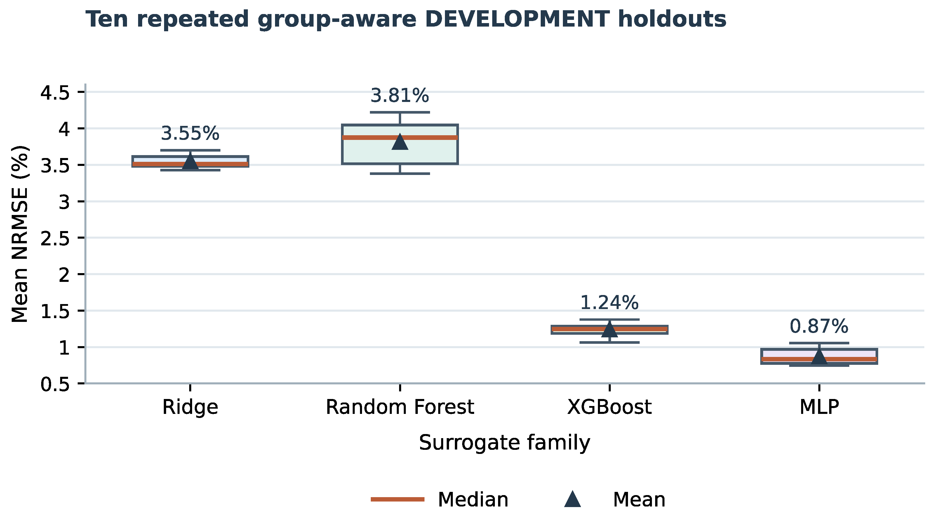
The repeated DEVELOPMENT experiment favored the MLP within the Base–Increment formulation in terms of global normalized regression error. Table 5 summarizes ten group-aware holdouts, while Figure 6 shows the NRMSE distributions across repetitions. The MLP achieved a mean NRMSE of 0.871% and the lowest NRMSE in all repetitions. XGBoost had the next-lowest mean NRMSE, while Ridge and RF produced larger errors. This comparison concerns model families using the same decomposition; a separate direct-MLP check is presented below.

Table 5. Repeated group-aware model-family comparison within DEVELOPMENT.

Family	Mean NRMSE (%)	NRMSE Std. (p.p.)	Median NRMSE (%)	Mean NMAE (%)	Mean ${\mathit{R}}^2$
MLP	0.8708	0.1195	0.8338	0.5988	0.9951
XGBoost	1.2409	0.0920	1.2474	0.8199	0.9901
Ridge	3.5470	0.0905	3.5114	2.4887	0.8968
Random Forest	3.8124	0.3056	3.8731	2.8273	0.8990

Figure 6. Distribution of NRMSE across repeated group-aware DEVELOPMENT partitions. Horizontal lines denote medians and triangles denote means.

After the MLP family and its hyperparameters were frozen and refitted on DEVELOPMENT, the independent TEST set was evaluated. Table 6 gives the physical-output metrics for the raw surrogate. NRMSE ranged from 0.103% for substation active power to 1.507% for active-power losses, while all reported $R^2$ values were at least 0.990. This strong average agreement does not establish whether individual predictions remain on the correct side of a voltage, loss, or loading limit.

Table 6. Independent TEST performance of the frozen raw Base–Increment MLP.

Output	MAE	RMSE	NRMSE (%)	Bias	${\mathit{R}}^2$
$V_{\min }$ (p.u.)	0.003182	0.003988	1.1498	0.000767	0.991397
$V_{\max }$ (p.u.)	0.001378	0.001886	0.6454	−0.000522	0.998263
$V_{\mathrm{DG},\max }$ (p.u.)	0.001546	0.002016	0.5579	−0.000176	0.998213
$P_{\mathrm{loss}}$ (kW)	8.335	13.835	1.5068	−2.842	0.990061
$L_{\max }$ (%)	2.015	2.568	1.1702	−0.571	0.992449
$P_{\mathrm{SE}}$ (kW)	7.594	10.932	0.1033	0.150	0.999910
$Q_{\mathrm{SE}}$ (kvar)	54.246	76.033	1.3352	−13.688	0.991538

3.2. Direct-MLP Architecture Check

As an additional architecture check, a direct MLP predicting the seven DG-state electrical outputs from the 24 input features was fitted using the same group-based dataset partitions. On the independent TEST partition, its train-range-normalized RMSE was lower for six of the seven outputs (Table 7), while the original Base–Increment representation retained a small advantage for substation active power. Thus, the decomposition does not provide a universal regression-accuracy advantage. Its original purpose was to support a common comparison across regression families, not to optimize the architecture specifically for MLP. The comparison was not strictly parameter- or hyperparameter-budget matched and is therefore a bounded architectural ablation, not a definitive ranking.

Table 7. Architecture ablation on independent TEST: train-range-normalized RMSE (%). Smaller values are better.

Electrical Output	Base–Increment	Direct MLP
$V_{\min }$	1.150	0.379
$V_{\max }$	0.645	0.415
$V_{\mathrm{DG},\max }$	0.558	0.281
$P_{\mathrm{loss}}$	1.507	0.317
$L_{\max }$	1.170	0.397
$P_{\mathrm{SE}}$	0.103	0.133
$Q_{\mathrm{SE}}$	1.335	0.314

Within TRAIN, the correlation between sampled active DG injection and baseline substation power was $r=0.469$ across 12,810 realizations and $r=0.934$ across 427 scenario-level means. Because baseline power is fixed within each group, these associations describe the scenario-dependent sampling design; they do not represent a physical DG effect on the baseline.

For a controlled feasibility comparison, both architectures were evaluated using the same predicted base state in the four constraints. Base–Increment yielded 17 false-feasible predictions (FFR 1.810%; recall 96.545%), whereas the direct MLP yielded 15 (FFR 1.667%; recall 92.670%). Group-paired bootstrap differences (direct minus Base–Increment) were −0.144 percentage points in FFR (95% interval [−1.073, 0.764]) and −3.874 percentage points in recall (95% interval [−5.519, −2.402]). The shared baseline allows comparison of with-DG predictions but does not constitute a fully autonomous direct-MLP deployment pipeline. Accordingly, the main contribution here is calibration of decision constraints, not predictive dominance of the Base–Increment architecture.

3.3. Constraint-Space Error Structure

Before applying calibration, the raw surrogate errors were also expressed directly in the four constraint functions. Table 8 shows that the largest raw false-feasible rate at the individual-constraint level occurred for the maximum-voltage constraint, with 2.10%, while the corresponding values for minimum voltage, active-power losses, and maximum conductor loading were 1.20%, 0.75%, and 1.07%, respectively. The proportions of optimistic and conservative residuals differed across constraints: for example, 64.58% of the $g_{V_{\max }}$ residuals were optimistic, whereas only 36.92% of the loss residuals were optimistic. This directional structure motivates the use of one-sided rather than symmetric corrections.

Table 8. Raw surrogate error statistics in constraint space on CALIBRATION. Positive oriented error denotes an optimistic surrogate error. MAE and RMSE retain each constraint’s physical unit.

Metric	${\mathit{g}}_{{\mathit{V}}_{\min }}$	${\mathit{g}}_{{\mathit{V}}_{\max }}$	${\mathit{g}}_{\mathbf{Loss}}$	${\mathit{g}}_{\mathbf{Loading}}$
MAE	0.000614	0.001398	1.498157	1.089198
RMSE	0.001195	0.001934	2.266649	1.908947
Optimistic (%)	43.178	64.579	36.916	46.729
Conservative (%)	56.822	35.421	63.084	53.271
FFR (%)	1.201	2.096	0.749	1.073
Recall (%)	99.681	98.866	96.262	98.181

3.4. Calibration Stability and Independent Feasibility Decisions

The repeated calibration experiment produced different levels of conservatism among the frozen strategies (Table 3). The final output-space and joint-vector configurations appeared in 10% and 15% of the repeated partitions, respectively. Uniform and constraint-specific were determined by their stated repeated-selection rules rather than simply choosing the most common full vector. This variability is why the repeated calibration analysis is treated as an internal selection-stability assessment rather than a formal uncertainty or future-feasibility guarantee.

On the independent TEST set, 955 of 3240 operating points were feasible according to the formal OpenDSS constraints and 2285 were infeasible. Table 9 shows the resulting classification metrics. The raw surrogate retained the largest recall (96.54%) but had the highest FFR (1.81%). Calibration reduced FFR, with different reductions in recall. Constraint-specific calibration yielded the lowest FFR (0.24%) but also the largest reduction in recall (85.55%). Output-space, uniform, and joint-vector calibration occupied intermediate parts of this trade-off.

Table 9. Independent TEST feasibility-classification performance. FFR is $FP/(TP+FP)$.

Strategy	TP	FP	TN	FN	FFR (%)	Recall (%)
Raw	922	17	2268	33	1.8104	96.5445
Output-space	886	5	2280	69	0.5612	92.7749
Uniform constraint	902	7	2278	53	0.7701	94.4503
Constraint-specific	817	2	2283	138	0.2442	85.5497
Joint-vector	902	9	2276	53	0.9879	94.4503

Uncertainty was assessed using 4000 paired bootstrap replicates of the 108 TEST base scenarios, retaining all 30 DG points within each resampled group. The 95% percentile FFR intervals were [0.964, 2.800]% (raw), [0.106, 1.239]% (output-space), [0.227, 1.451]% (uniform), [0.000, 0.635]% (constraint-specific), and [0.362, 1.718]% (joint-vector). The corresponding recall intervals were [95.312, 97.633]%, [90.886, 94.538]%, [92.698, 96.068]%, [82.495, 88.321]%, and [92.646, 96.054]%. All four paired FFR differences relative to raw had intervals below zero.

The FFR–recall trade-off summarized in Table 9 has no uniformly dominant calibrated strategy. Pairwise FFR differences between output-space and uniform ($[-0.654,0.225]$ percentage points) and between uniform and joint-vector ($[-0.758,0.306]$) were not clearly separated from zero. Output-space had lower recall than uniform ($[-2.909,-0.512]$ percentage points for their difference). These grouped bootstrap intervals describe sampling variability in the studied network; they are exploratory, unadjusted for multiple comparisons, and not feasibility guarantees.

The maximum normalized violation among the false-feasible TEST cases also remained limited in this sample: median/maximum values were 0.0171/0.0958 (raw, $n=17$), 0.0181/0.0958 (output-space, $n=5$), 0.0181/0.0400 (uniform, $n=7$), 0.0189/0.0365 (constraint-specific, $n=2$), and 0.0143/0.0400 (joint-vector, $n=9$). These dimensionless descriptive diagnostics are separate from the physical-unit HC violations reported in Section 3.5. Among the 17 distinct false-feasible TEST operating points accepted by at least one strategy, the largest positive OpenDSS violations were 0.005442 p.u. ($g_{V_{\max }}$), 2.071 kW ($g_{\mathrm{Loss}}$), and $3.79\times {10}^{-8}$ p.u. ($g_{V_{\min }}$); none violated $g_{\mathrm{Loading}}$. These maxima are pooled across strategies, not separate maxima for every calibration.

All false-feasible TEST decisions were close to an OpenDSS constraint boundary: the normalized distance to the nearest violated boundary was below 0.10, with a median below 0.02 for every strategy. Thus, the remaining optimistic feasibility decisions were concentrated near technical limits rather than broadly dispersed across the infeasible region. This proximity diagnostic does not measure worst-case severity, which is assessed separately using the maximum normalized violation reported above.

3.5. Hosting-Capacity Results and OpenDSS Verification

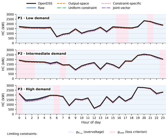
The common HC engine was applied to all 72 hourly conditions using OpenDSS and each surrogate strategy. No OpenDSS result reached the 4500 kW censoring limit. Figure 7 compares the hourly HC trajectories for the low-, intermediate-, and high-demand profiles, with pale-blue and pale-pink background shading indicating the recorded OpenDSS limiting constraints (upper voltage and losses, respectively); Figure 8 shows the corresponding surrogate errors.

Figure 7. Hourly hosting capacity obtained with OpenDSS and the raw and calibrated surrogate strategies for the three 2026 demand profiles. Background shading identifies the limiting-constraint labels recorded in the OpenDSS HC search: pale blue, upper-voltage limit ($g_{V_{\max }}$); pale pink, no-increase loss criterion ($g_{\mathrm{Loss}}$).

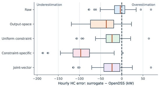
Figure 8. Distribution of hourly HC error, defined as surrogate minus OpenDSS, across the 72 evaluated hourly conditions.

Table 10 summarizes hourly HC agreement. The raw surrogate had the smallest numerical error (MAE 18.85 kW; MAPE 1.225%) but overestimated the OpenDSS reference by more than 0.5 kW in 43.06% of the 72 hourly cases. Output-space reduced that frequency to 8.33%, while uniform and joint-vector yielded 15.28% and 18.06%, respectively. Constraint-specific nearly eliminated hourly overestimation (1.39%) but was more conservative, retaining 93.54% of mean reference HC and giving the largest MAE. Figure 8 illustrates the distributions of signed HC errors (surrogate minus OpenDSS; negative values denote underestimation). Raw had P05, median, and P95 errors of $-55.50$, $-3.50$, and $27.35$ kW, respectively, whereas constraint-specific had $-158.05$, $-97.00$, and $-41.20$ kW. These distributions illustrate how smaller average errors can coexist with more frequent HC overestimation.

Table 10. Hourly HC agreement with OpenDSS over 72 conditions. Positive bias denotes average overestimation.

Metric	Raw	Output-Space	Uniform	Constraint-Specific	Joint-Vector
MAE (kW)	18.847	45.278	28.181	96.264	30.875
RMSE (kW)	26.293	54.802	36.898	102.632	40.491
MAPE (%)	1.225	2.764	1.846	6.459	2.061
Bias (kW)	−6.208	−43.583	−23.958	−96.208	−26.347
Overest. (%)	43.056	8.333	15.278	1.389	18.056
Max overest. (kW)	69	23	64	2	69
Mean HC retained (%)	99.223	97.309	98.270	93.543	98.053

The stored OpenDSS HC-search labels identify overvoltage as the limiting condition in 62 of 72 h and the no-increase loss criterion in the remaining 10. In this fixed-bus, unity-power-factor case, additional active injection most often reaches the absolute upper-voltage threshold before the other adopted criteria; in the remaining labeled hours, the original search instead identified the deliberately conservative loss test as limiting.

For a fixed DG installation, the relevant quantity is the 24 h capacity evaluated across all 24 h under the corresponding feasibility criteria, as defined in Equation (16). Table 11 gives those values. OpenDSS produced 662, 933, and 617 kW for the low-, intermediate-, and high-demand profiles. At this 24 h aggregation level, raw exceeded the reference for P1 and P3, while joint-vector and constraint-specific remained below it in all three profiles. These profile-level results should not be conflated with the 72 h accuracy ranking.

Table 11. Fixed 24 h HC candidates verified jointly against each evaluator’s constraints (kW). Independent OpenDSS validation of surrogate-selected capacities is reported in the text.

Profile	OpenDSS	Raw	Output	Uniform	Constraint-Specific	Joint-Vector
P1–Low demand	662	685	665	657	578	648
P2–Intermediate demand	933	923	903	894	816	886
P3–High demand	617	651	631	622	543	614

Only three demand trajectories were examined; these 24 h values are descriptive rather than evidence of annual or multi-feeder performance. At the fixed 24 h level, output-space has the smallest MAE (15.67 kW), whereas raw has the smallest MAE across 72 individual hours (18.85 kW).

3.6. Independent OpenDSS Verification

Two complementary questions were evaluated: how closely a surrogate estimates the reference HC, and whether the capacity it selects actually satisfies the OpenDSS constraints. An HC estimate can match the reference at the final 1 kW resolution yet fail a separate feasibility check if a constraint residual lies extremely close to zero. Therefore, all 360 surrogate-selected hourly capacities (five strategies times 72 conditions) were independently re-evaluated with OpenDSS.

Table 12 reports 64 infeasible selections using the original ${10}^{-10}$ numerical comparison. Of these, 33 violated upper voltage and 33 violated the loss criterion; two violated both, giving 64 distinct cases. There were no violations of minimum voltage or loading. An exploratory ${10}^{-8}$ p.u. allowance on upper voltage alone reclassified one excess of $4.91\times {10}^{-9}$ p.u., reducing the count to 63.

Table 12. Independent OpenDSS verification of surrogate-selected hourly HC, using the original numerical comparison (${10}^{-10}$ in the respective constraint units); 72 conditions per strategy.

Strategy	Feasible	Infeasible	Infeasible (%)
Raw	40	32	44.44
Output-space	66	6	8.33
Uniform constraint	61	11	15.28
Constraint-specific	71	1	1.39
Joint-vector	58	14	19.44

A capacity was counted infeasible under the original ${10}^{-10}$ comparison of each constraint to zero. Because $g_j$ has different units, this small code tolerance is a classification convention, not a demonstrated engineering or solver-accuracy tolerance; the isolated ${10}^{-8}$ p.u. voltage sensitivity is reported separately. Across raw, output-space, uniform, constraint-specific, and joint-vector, respectively, maximum upper-voltage exceedances were 0.002457, 0.000804, 0.002281, 0.000040, and 0.002460 p.u.; maximum loss-limit exceedances were 2.444, 0, 2.057, 0, and 2.468 kW. These values apply to selected HC candidates, not all TEST samples.

A separate OpenDSS check applied each of the 15 surrogate-selected fixed 24 h capacities to all 24 h (360 evaluations), after all 18 selected capacities had been confirmed feasible by their own evaluators. The number of infeasible hours was two (raw), two (output-space), one (uniform), zero (constraint-specific), and zero (joint-vector); all five failures were due to the upper-voltage constraint. Each infeasible hourly evaluation belonged to a different strategy–profile combination; consequently, five distinct fixed capacities failed at least one hourly check, with exactly one infeasible hour per affected capacity. The TEST-set FFR concerns infeasible OpenDSS points among the surrogate-accepted classification samples, whereas hourly HC overestimation counts positive capacity errors among 72 search outcomes; their denominators and operating-point selection differ. Three dense 1 kW OpenDSS sweeps (0–4500 kW) reproduced the original search results for the three selected hourly conditions (1727, 1664, and 1618 kW). These spot checks validate the search locally but do not establish global optimality for every other hour or DG location.

3.7. Computational Performance

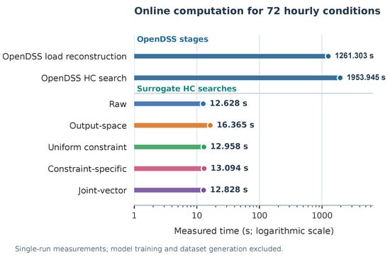
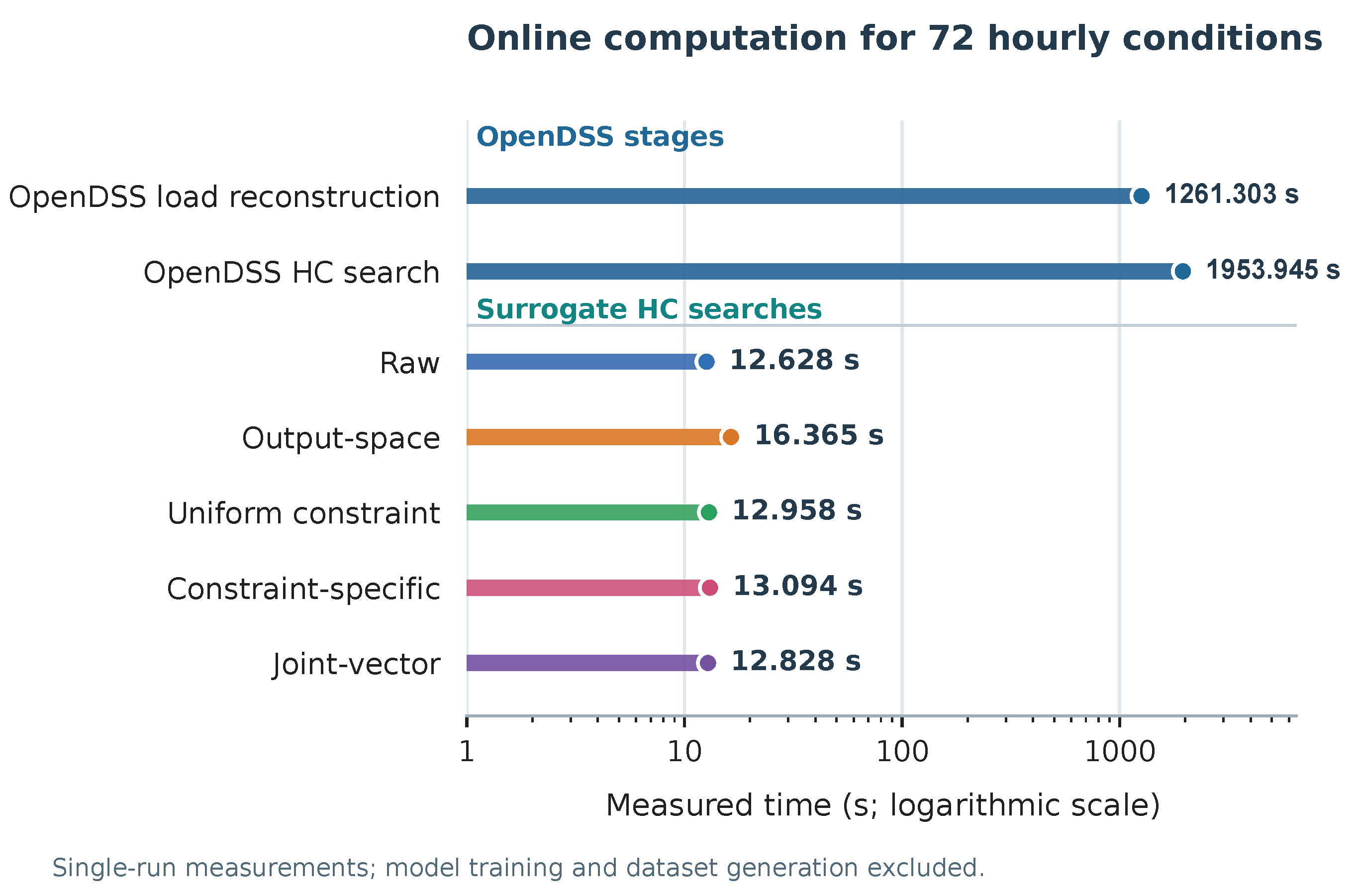
The computation-time breakdown for all 72 hourly conditions is summarized in Table 13. OpenDSS required 1261.30 s to reconstruct the 72 base load conditions and 1953.95 s for the HC searches, for an online workflow total of 3215.25 s. The surrogate strategies required between 12.63 and 16.36 s for the same 72 HC searches. Depending on the calibration strategy, search-only speedup ranged from 119.4× to 154.7×, while workflow speedup ranged from 196.5× to 254.6×.

Table 13. Online HC-search timing for 72 conditions. Common OpenDSS references: load reconstruction 1261.303 s and HC search 1953.945 s.

Strategy	Surrogate Search (s)	Search Speedup	Workflow Speedup
Raw	12.628	154.74×	254.62×
Output-space	16.365	119.40×	196.47×
Uniform constraint	12.958	150.79×	248.12×
Constraint-specific	13.094	149.22×	245.54×
Joint-vector	12.828	152.32×	250.64×

The computational comparison concerns online assessment after surrogate training and calibration. The distinction between load reconstruction and HC search matters because OpenDSS must establish the spatial allocation of hourly demand before evaluating DG candidates, whereas the trained surrogate consumes the operating-condition descriptors directly. As Figure 9 shows, the reported 119–155× speedups refer to HC search alone; the corresponding workflow comparison additionally includes the OpenDSS hourly load-reconstruction stage.

Figure 9. Measured online computation times for 72 hourly HC conditions: OpenDSS load reconstruction and search versus surrogate HC searches after training and calibration. The horizontal axis uses a logarithmic scale.

Offline computational stages, including dataset generation, model selection, and final MLP refitting, are documented separately in Appendix D. Because their execution times depend on the model-selection protocol, hyperparameter-search budget, and computational resources, the performance comparison focuses on the measured online HC-search workflow. All surrogate strategies achieved substantial computational savings relative to OpenDSS under the evaluated setup. The slightly longer execution time observed for output-space is reported as a workflow-level result rather than attributed to a specific operation. The retained notebooks and scenario-level outputs support the traceability of the reported results, subject to utility-data restrictions.

4. Discussion

The results reinforce the distinction between regression accuracy and decision reliability. The frozen Base–Increment MLP achieved low global prediction errors on independent TEST data, and the raw surrogate produced the smallest hourly HC error. Nevertheless, raw HC exceeded the OpenDSS reference in 43.06% of the evaluated hours. This is not contradictory: HC is determined close to technical feasibility boundaries, where errors small relative to the full range of an electrical variable can change which DG candidate is accepted. The engineering consequence of a prediction error therefore depends on its direction and its position relative to an operating limit.

The independent TEST classification provides the same evidence at the constraint-decision level. Raw produced an FFR of 1.81%, whereas all calibrated strategies lowered FFR with varying losses of recall. Constraint-specific yielded the lowest FFR (0.24%) and the greatest reduction in recall (85.55%). Output-space obtained 0.56% FFR and 92.77% recall; uniform and joint-vector both retained 94.45% recall, with FFR values of 0.77% and 0.99%. Grouped bootstrap comparisons do not establish a consistent ordering among all calibrated alternatives. These results are better interpreted as different operating trade-offs than as evidence for one generally optimal calibration strategy. For a distribution-system operator, the preferable choice depends on the consequences of accepting an infeasible condition versus rejecting a feasible one.

The boundary analysis shows that false-feasible TEST decisions were concentrated near the adopted electrical constraint limits, where small prediction errors can change feasibility classifications. The maximum normalized violation was also evaluated to account for potentially larger violations of other constraints. These findings highlight the importance of assessing surrogate reliability through decision-oriented metrics alongside conventional regression measures such as MAE, RMSE, and $R^2$.

The downstream HC results further expose this trade-off. Raw retained 99.22% of the hourly OpenDSS HC on average but frequently overestimated the admissible capacity. At the other extreme, constraint-specific reduced hourly overestimation to 1.39% with a maximum positive error of 2 kW, but mean retained HC fell to 93.54% and MAPE rose to 6.46%. The three 24 h demand profiles also show that HC cannot be inferred from mean daily demand alone: the intermediate-demand trajectory had the largest jointly verified OpenDSS HC (933 kW), while the high-demand trajectory had 617 kW. The critical electrical state and the complete set of adopted constraints determine the selected capacity. All 18 fixed-capacity candidates passed each evaluator’s own 24 h feasibility check, but 5 of the 15 surrogate-selected fixed capacities violated the OpenDSS upper-voltage limit. At the 24 h aggregation level, output-space achieved the lowest MAE (15.67 kW), although two of its three fixed-capacity estimates failed the independent OpenDSS feasibility check. These values are candidates from the specified search, not globally certified maxima of a continuous nonmonotone domain.

The online computational benefit remains substantial under the common search procedure. Across the 72 hourly conditions, surrogate HC searches were 119–155× faster than OpenDSS HC searches. Including the OpenDSS hourly load-reconstruction step increased the observed workflow speedup to 196–255×. These results characterize the measured online HC workflow, while offline activities such as dataset generation, hyperparameter tuning, model fitting, and calibration are documented separately in Appendix D.

Several limitations define the scope of the findings. The study considers one detailed distribution network, a fixed DG connection point, and a constant topology. The three P5/P50/P95 demand profiles represent alternative operating conditions for a single date, rather than independent days or annual variability, while the illustrative HC assessment assumes $Q_{\mathrm{DG}}=0$. Changes in DG location, network topology, Volt–Var control, or inverter reactive-power dispatch may modify the constraint boundaries and prediction-error distributions, requiring additional validation and potentially recalibration. Harmonics, explicit voltage-unbalance indices, and inverter dynamics are outside the steady-state acceptance criteria considered in this study [30]. Furthermore, the empirical quantile margins are designed to evaluate the observed FFR–recall trade-off rather than provide formal split-conformal coverage or conformal risk-control guarantees [24,31]. Extending the framework to these operating conditions and formal risk-control methods constitutes a direction for future research.

Future work should examine additional feeders and DG locations, longer operating horizons, reactive-power control, and alternative network topologies. Because the surrogate preserves continuous electrical outputs, it can also support operational screening of voltage, losses, and loading alongside load and renewable-generation forecasts, provided that feasibility is revalidated under the intended deployment conditions.

5. Conclusions

This study evaluated the reliability of a continuous-output power-flow surrogate when its predictions are used to make engineering decisions under electrical constraints. The Base–Increment MLP achieved a mean DEVELOPMENT NRMSE of 0.871%, while TEST NRMSE ranged from 0.103% to 1.507%. Despite this predictive accuracy, the uncalibrated model accepted operating conditions that violated the OpenDSS constraints. The direct-MLP comparison did not establish predictive superiority of the Base–Increment architecture, reinforcing that the principal contribution of this work lies in the evaluation and calibration of constraint-based decisions rather than in the surrogate architecture itself.

The four empirical calibration strategies reduced false-feasible decisions, although with different effects on the retention of feasible operating conditions. On the independent TEST partition, FFR decreased from 1.81% for the raw surrogate to 0.24–0.99% for the calibrated strategies, with recall ranging from 85.55% to 94.45%. The remaining false-feasible predictions were concentrated near electrical constraint boundaries, demonstrating why low regression errors alone are insufficient to characterize decision reliability.

The illustrative HC assessment further demonstrated the practical implications of these differences. Although raw achieved the lowest hourly HC MAPE (1.225%), it overestimated the OpenDSS reference in 43.06% of the hourly comparisons. More importantly, independent OpenDSS verification of the 72 hourly HC selections per strategy identified 32 infeasible selections for raw (44.44%), compared with 6 for output-space (8.33%), 11 for uniform constraint-space (15.28%), 1 for constraint-specific (1.39%), and 14 for joint-vector calibration (19.44%), under the adopted numerical feasibility criterion. These results demonstrate that improved predictive accuracy and lower test-set FFR do not translate proportionally into improved HC decisions. At the fixed 24 h level, 5 of the 15 surrogate-selected capacities failed independent OpenDSS verification, each with one infeasible hourly evaluation among its 24 operating conditions, despite satisfying the constraints according to its surrogate evaluator.

The HC results also revealed a non-proportional relationship between demand conditions and the admissible DG capacity. OpenDSS obtained fixed 24 h capacities of 662, 933, and 617 kW for the low-, intermediate-, and high-demand profiles, respectively. The intermediate-demand profile therefore supported the highest capacity, rather than following a monotonic progression across demand levels. This behavior reflects the interaction between hourly load patterns, network operating conditions, and the adopted electrical constraints. In particular, upper-voltage limits were identified as the limiting condition in 62 of the 72 hourly OpenDSS searches, with the conservative no-increase loss criterion limiting the remaining 10. These findings emphasize that HC depends on the temporal characteristics of demand and the active network constraints, rather than on demand magnitude alone.

The computational assessment confirmed the practical potential of the calibrated surrogates. HC searches were 119–155× faster than OpenDSS, increasing to 196–255× when the hourly OpenDSS load-reconstruction step was included in the measured online workflow. Overall, the results demonstrate the importance of incorporating decision-oriented calibration and independent constraint verification into surrogate-based distribution-system studies. The proposed framework provides an empirical approach for examining the trade-off between feasibility reliability, retained HC, and computational efficiency, while its extension to other networks, DG locations, and operating conditions remains an opportunity for further investigation.

References

- Fatima, S.; Püvi, V.; Lehtonen, M. Review on the PV Hosting Capacity in Distribution Networks. Energies 2020, 13, 4756. [Google Scholar] [CrossRef] [Scilit]
- Qamar, N.; Arshad, A.; Mahmoud, K.; Lehtonen, M. Hosting Capacity in Distribution Grids: A Review of Definitions, Performance Indices, Determination Methodologies, and Enhancement Techniques. Energy Sci. Eng. 2023, 11, 1536–1559. [Google Scholar] [CrossRef] [Scilit]
- Benzerga, A.; Bahmanyar, A.; Derval, G.; Ernst, D. A Unified Definition of Hosting Capacity, Applications, and Review. IEEE Access 2025, 13, 7819–7836. [Google Scholar] [CrossRef] [Scilit]
- Karmaker, A.K.; Du, Y.; Yang, J.; Jacob, M.V. Challenges and Applications of Hosting Capacity Analysis in DER-Rich Power Systems. Appl. Energy 2026, 407, 127323. [Google Scholar] [CrossRef] [Scilit]
- L. do Nascimento, A.L.; Santana de Albuquerque, B.; Freitas da S. Junior, H.; M. Rodrigues, C.E.; Moura de Moura Carvalho, C.C.; H. Bezerra, U.; Muñoz Tabora, J.; de Lima Tostes, M.E. Topology-Aware Assessment of Voltage Regulation and Continuous Photovoltaic Hosting Capacity in PV-Rich Distribution Feeders with Smart-Inverter Controls. Electricity 2026, 7, 78. [Google Scholar] [CrossRef] [Scilit]
- Villa-Ávila, E.; Arévalo, P.; Aguado, R.; Ochoa-Correa, D.; Iñiguez-Morán, V.; Jurado, F.; Tostado-Véliz, M. Enhancing Energy Power Quality in Low-Voltage Networks Integrating Renewable Energy Generation: A Case Study in a Microgrid Laboratory. Energies 2023, 16, 5386. [Google Scholar] [CrossRef] [Scilit]
- Carmona, C.; Romero-Ramos, E.; Riquelme, J.; Gómez-Expósito, A. Distribution Transformer Load Allocation from Substation Measurements and Load Patterns. In Proceedings of the IEEE PES Innovative Smart Grid Technologies Conference Europe, Gothenburg, Sweden, 11–13 October 2010. [Google Scholar] [CrossRef] [Scilit]
- Frost, A.E.; Azaza, M.; Li, H.; Wallin, F. Patterns and Temporal Resolution in Commercial and Industrial Typical Load Profiles. Energy Procedia 2017, 105, 2684–2689. [Google Scholar] [CrossRef] [Scilit]
- Wan, J.; Miu, K.N. Weighted Least Squares Methods for Load Estimation in Distribution Networks. IEEE Trans. Power Syst. 2003, 18, 1338–1345. [Google Scholar] [CrossRef] [Scilit]
- Balduin, S.; Tröschel, M.; Lehnhoff, S. Towards Domain-Specific Surrogate Models for Smart Grid Co-Simulation. Energy Inform. 2019, 2, 27. [Google Scholar] [CrossRef] [Scilit]
- Balduin, S.; Westermann, T.; Puiutta, E. Evaluating Different Machine Learning Techniques as Surrogate for Low Voltage Grids. Energy Inform. 2020, 3, 24. [Google Scholar] [CrossRef] [Scilit]
- Ivanov, O.; Bontea, A.J.; Grigoras, G.; Baciu, M.A.; Gavrilas, M. Load Flow Calculation in Electricity Distribution Systems Using Artificial Neural Networks. In Proceedings of the 12th International Conference on Energy and Environment (CIEM), Bucharest, Romania, 23–24 October 2025. [Google Scholar] [CrossRef] [Scilit]
- Yeptho, P.; Saldaña-González, A.E.; Aragüés-Peñalba, M.; Barja-Martínez, S. Evaluation of XGBoost and ANN as Surrogates for Power Flow Predictions with Dynamic Energy Storage Scenarios. Energies 2025, 18, 4416. [Google Scholar] [CrossRef] [Scilit]
- Pjetri, G.; Mohapatra, A.; Baecker, B.R.; Hock, M.; Hamacher, T. Graph Neural Network Surrogates for Energy System Modeling. In Proceedings of the IEEE PES Innovative Smart Grid Technologies Conference Europe, Valletta, Malta, 20–23 October 2025. [Google Scholar] [CrossRef] [Scilit]
- Kaseb, Z.; Orfanoudakis, S.; Vergara, P.P.; Palensky, P. Physics-Informed Neural Network with Adaptive Activation for Power Flow. Int. J. Electr. Power Energy Syst. 2026, 174, 111525. [Google Scholar] [CrossRef] [Scilit]
- Ma, A.; Ghamizi, S.; Bojchevski, A.; Zhang, P.; Cao, J. SafePowerGraph: A Safety-Aware Benchmarking Framework for Scalable Graph Neural Networks in Power Flow and Optimal Power Flow. Energy AI 2026, 25, 100819. [Google Scholar] [CrossRef] [Scilit]
- Qammar, N.; Arshad, A.; Miller, R.J.; Mahmoud, K.; Lehtonen, M. Machine Learning Based Hosting Capacity Determination Methodology for Low Voltage Distribution Networks. IET Gener. Transm. Distrib. 2024, 18, 911–920. [Google Scholar] [CrossRef] [Scilit]
- Siddique, M.N.I.; Prakash, K.; Mekhilef, S.; Pota, H. Real-Time PV Hosting Capacity Analysis of Distribution Networks Using Pilot Buses Data and Neural Networks. Appl. Energy 2026, 409, 127467. [Google Scholar] [CrossRef] [Scilit]
- Yan, Z.; Liu, J.; Zhang, D.; Liu, D.; Feng, Y.; Shu, J. Dynamic Hosting Capacity Assessment of Photovoltaics in Distribution Networks Considering Static Voltage Stability Margin. Front. Energy Res. 2026, 14, 1916798. [Google Scholar] [CrossRef] [Scilit]
- Talbi, B.; Derri, M.; Haidi, T.; Mahrouch, H. Photovoltaic Hosting Capacity Assessment and Violation Prediction in Electrical Distribution Networks. Electr. Power Syst. Res. 2026, 255, 112815. [Google Scholar] [CrossRef] [Scilit]
- Ma, H.; Li, G.; Wang, H.; Yan, Z.; Xu, X. Probabilistic Evaluation of Photovoltaic Hosting Capacity in Unbalanced Distribution Network via Polynomial Chaos Based Kriging Model. IEEE Trans. Ind. Appl. 2025, 61, 1466–1474. [Google Scholar] [CrossRef] [Scilit]
- Ly, S.; Singh, A.; Vorobev, P.; Soh, Y.C.; Nguyen, H.D. Chance-Constrained Solar PV Hosting Capacity Assessment for Distribution Grids Using Gaussian Process and Logit Learning. Int. J. Electr. Power Energy Syst. 2025, 170, 110783. [Google Scholar] [CrossRef] [Scilit]
- Wang, Z.; Jia, Y.; Han, X.; Wang, P.; Liu, J. Deep Learning-Based Distributionally Robust Joint Chance Constrained Distribution Networks PV Hosting Capacity Assessment. Appl. Energy 2025, 394, 126130. [Google Scholar] [CrossRef] [Scilit]
- Angelopoulos, A.N.; Bates, S. Conformal Prediction: A Gentle Introduction. Found. Trends Mach. Learn. 2023, 16, 494–591. [Google Scholar] [CrossRef] [Scilit]
- Romano, Y.; Patterson, E.; Candès, E.J. Conformalized Quantile Regression. In Advances in Neural Information Processing Systems; Curran Associates, Inc.: Red Hook, NY, USA, 2019; Volume 32, Available online: https://proceedings.neurips.cc/paper_files/paper/2019/hash/5103c3584b063c431bd1268e9b5e76fb-Abstract.html (accessed on 29 September 2026).
- Barber, R.F.; Candès, E.J.; Ramdas, A.; Tibshirani, R.J. Conformal Prediction Beyond Exchangeability. Ann. Stat. 2023, 51, 816–845. [Google Scholar] [CrossRef] [Scilit]
- Shamseldein, M. Learned Surrogates for AC Feasibility in Stochastic Unit Commitment: A Comparative Study with Conformal Guarantees. IET Gener. Transm. Distrib. 2026, 20, e70345. [Google Scholar] [CrossRef] [Scilit]
- Chiguano Velasco, A.N.; Rentería Bustamante, L.F. Modelo de optimización no lineal para estimación de perfiles de carga en sistemas eléctricos de distribución. Rev. Ingenio Glob. 2024, 3, 91–118. [Google Scholar] [CrossRef] [Scilit]
- Agencia de Regulación y Control de Electricidad (ARCONEL). Regulación Nro. ARCONEL-009/2024 (Codificada): Calidad del Servicio de Distribución y Comercialización de Energía Eléctrica; Anexo a la Resolución Nro. ARCONEL-030/2025, 31 de Diciembre de 2025; ARCONEL: Quito, Ecuador, 2025. Available online: https://arconel.gob.ec/wp-content/uploads/downloads/2026/02/Resolucion_nro_arconel-030-2025_reforma_a_la_regulacion_nro._arconel-009-2024_certificada-signed.pdf (accessed on 29 September 2026).
- Garcia-Uzca, C.; Ochoa-Correa, D. Power Quality in Grid-Connected Photovoltaic Inverters: A Systematic Review of Critical Parameters, Standards, and Mitigation Strategies. IEEE Access 2026, 14, 141821–141848. [Google Scholar] [CrossRef] [Scilit]
- Angelopoulos, A.N.; Bates, S.; Fisch, A.; Lei, L.; Schuster, T. Conformal Risk Control. In Proceedings of the International Conference on Learning Representations (ICLR), Vienna, Austria, 7–11 May 2024; Available online: https://proceedings.iclr.cc/paper_files/paper/2024/hash/f3549ef9b5ff520a7e41ff3cc306ab2b-Abstract-Conference.html (accessed on 29 September 2026).
Disclaimer/Publisher’s Note: The statements, opinions and data contained in all publications are solely those of the individual author(s) and contributor(s) and not of MDPI and/or the editor(s). MDPI and/or the editor(s) disclaim responsibility for any injury to people or property resulting from any ideas, methods, instructions or products referred to in the content. |
© 2026 by the authors. Licensee MDPI, Basel, Switzerland. This article is an open access article distributed under the terms and conditions of the Creative Commons Attribution (CC BY) license.