


Abstract
This article presents a novel control method, modified dynamic surface control (MDSC), developed based on the well-established dynamic surface control (DSC) framework to enhance the performance of strictly parametric feedback nonlinear systems. The proposed method retains the core advantages of DSC while introducing a sign function into the virtual control signal at each design step, effectively reducing transient time, improving response characteristics, and simplifying the overall control design process. By addressing one of the key limitations of traditional DSC—its sensitivity to dynamic uncertainties—the MDSC approach enhances system robustness and ensures smoother control performance. To validate its effectiveness, the proposed method is applied to control the rotational speed of a switched reluctance motor (SRM), a highly nonlinear electromechanical system with strong parameter variations. Extensive simulation results demonstrate that MDSC achieves superior tracking accuracy, faster convergence, and improved system stability compared to conventional DSC approaches. These findings highlight the potential of MDSC as an efficient and practical solution for high-performance nonlinear control applications, particularly in complex electromechanical systems where precision and adaptability are critical.
1. Introduction
Switched reluctance motors (SRMs) are increasingly gaining attention in both academic research and industrial applications due to their numerous advantages, including low manufacturing cost, high durability, and excellent noise tolerance. These characteristics make SRMs a promising alternative to traditional motor technologies, particularly in cost-sensitive and high-reliability applications. However, despite these benefits, SRMs still present significant challenges that hinder their widespread adoption. Their inherently high torque ripple, strong vibrations, and elevated noise levels make precise control difficult, requiring advanced control strategies to achieve stable and efficient operation. These limitations have driven extensive research efforts aimed at enhancing the performance and applicability of SRMs. Recent studies in this field have primarily focused on two key directions: improving the SRM mathematical model [1,2,3] to achieve more accurate system representation and predictive capabilities, and developing novel control algorithms [4,5] to mitigate torque ripple, enhance efficiency, and ensure smoother operation. Given the increasing demand for high-performance electric motors in modern applications such as electric vehicles, robotics, and renewable energy systems, advancing SRM technology is more critical than ever. Therefore, further innovations in both modeling techniques and control methodologies are essential to unlocking the full potential of SRMs and making them a viable solution for next-generation electromechanical systems.
In the first direction, documents [2,3] studied in detail the structure and magnetization characteristics of the SRM iron core but did not consider the switch model and power supply circuit—two important components that create the rotating magnetic field and electromagnetic torque for the rotor. Rigatos et al. [1] improved the SRM model by integrating the switch model into the SRM electromechanical model, but the assumption of instantaneous on/off switches is only suitable for small-capacity SRMs. With large-power motors, the charge-discharge time of the semiconductor valve is significant, negatively affecting the control system [6].
In the second direction, studies mainly aim at stable speed control [4,5,6,7] and improving the quality of output torque [5,8,9,10]. SRM control algorithms are quite diverse, from linear to nonlinear control such as the sliding technique [11,12,13,14] and the Backstepping technique [4,15,16,17]. The backstepping technique has been applied to SRM [4,15,16,17] to stabilise the speed. However, this method cannot completely eliminate high-frequency vibration and is affected by noise during the switching process of phases.
To solve this problem, a low-pass filter (LPF) has been integrated, creating the dynamic surface control (DSC) method, which reduces vibration and simplifies the calculation process [8]. DSC also stabilises the system using Lyapunov functions, which is suitable for SRM when operating in switching mode. Although traditional control methods have improved the performance of SRM, they are still limited in achieving high accuracy and short response time. This is the motivation for the research and development of advanced control methods such as dynamic surface control (DSC). This paper will focus on presenting the improved DSC method and evaluating its effectiveness through detailed simulations. The analysis results will provide insights into the applicability of the Modified DSC method in improving the performance of SRM, opening up new development directions for motor control technology in the future.
The paper is structured as follows: Section 2 presents the structure, the mathematical description of SRM and the speed control problem; Section 3 designs an improved DSC controller for SRM; Section 4 is the simulation and evaluation of the results; and the conclusion and development direction are presented at the end.
2. Switched Reluctance Machine Description
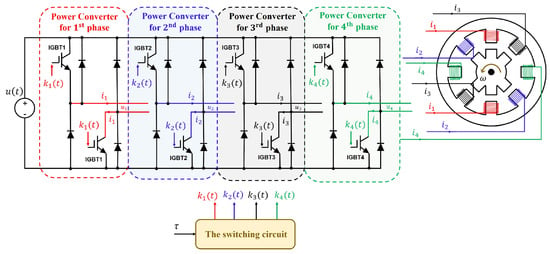
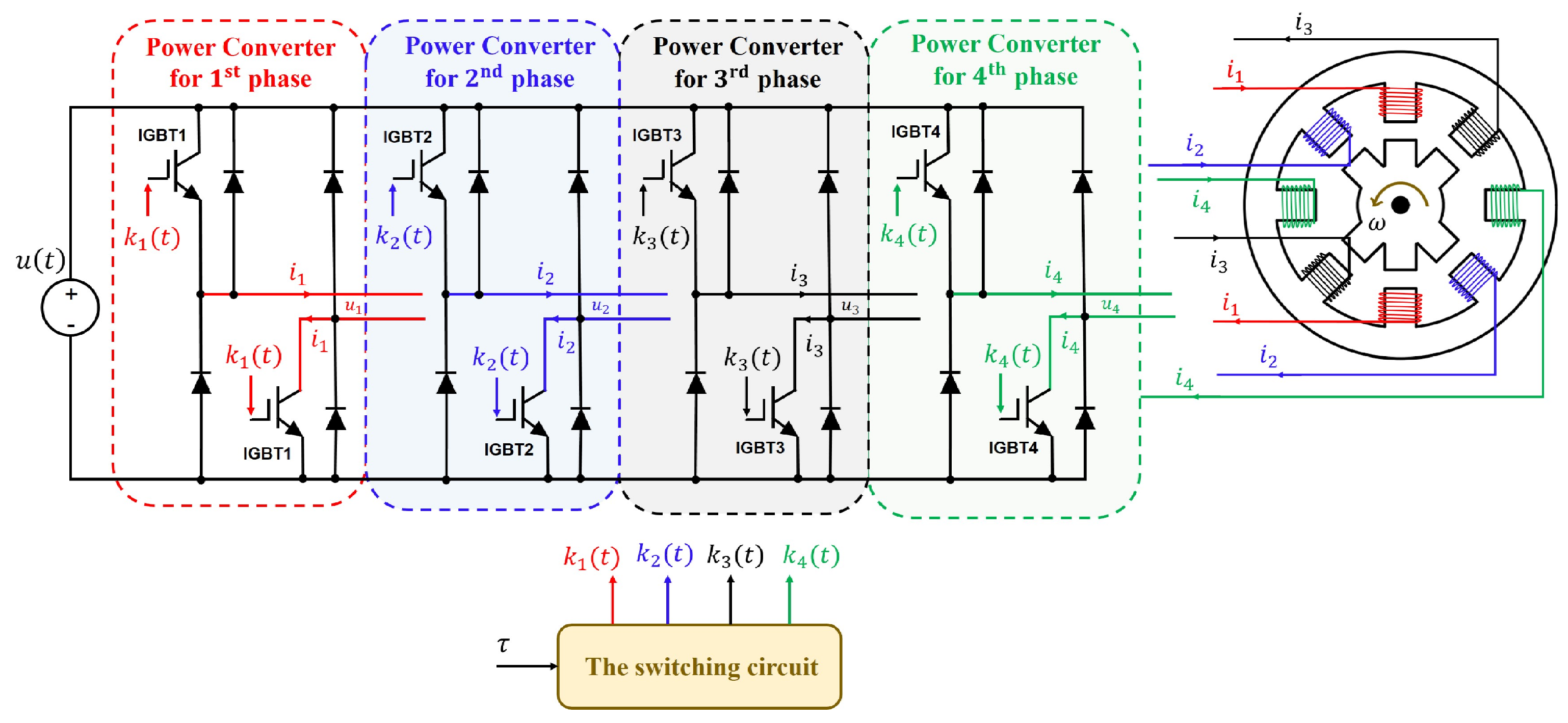
Figure 1 depicts the structure of the SRMs including the rotor and stator. The rotor-stator diagram of the SRM system shown in Figure 1 has 8 poles in the stator and 6 poles in the rotor. Thus, the studied SRMs here are also called the 8/6 SRMs system. In addition, the SRM system has four independent phases in which the independent voltages supplied for each phase are symbolised by . The voltages supplied for each phase are navigated by voltage-source power converters where the operation of Diodes and IGBTs is controlled by the generated-holding impulses. The values of the currents in each phase are denoted by and , respectively. The position of the SRM’s rotor is symbolised by . The first-order derivation of is , which is the rotational speed of the SRM system. Albeit four phases of the SRM system, only one phase is supplied voltage at a certain instant. Moreover, due to the salient pole configurations in both 8/6 SRMs’ rotor and stator, the position of the rotor has strong nonlinearities.
Figure 1.
The 8/6-SRMs configuration and its voltage-source power converters in [8].
Compared to conventional 6/4 structures, the 8/6 topology features a smaller step angle of , which inherently increases the phase overlap region during commutation and facilitates a significant reduction in torque ripple [3]. This enhanced geometric layout provides a smoother torque profile. Furthermore, configured as a four-phase machine, the 8/6 SRM exhibits exceptional fault tolerance; the electrical, magnetic, and thermal isolation between adjacent phases ensures that the drive can maintain partial torque production even under open-circuit or short-circuit faults [18]. Due to the absence of permanent magnets and rotor windings, the mechanical robustness of the 8/6 salient rotor prevents thermal demagnetisation and withstands high centrifugal stress, thereby rendering it ideal for high-speed, safety-critical actuators in autonomous vehicles and harsh industrial environments [19].
From a control perspective, are the input signals of the SRM system, which is designed to make the rotational speed stable at the desired value. By defining the vector of the states in which , , , , and , the mathematical description of the 8/6 SRM system is determined as follows [1]:
where . is the torque of the load. is the resistance of the winding on the SRM’s stator depending upon its temperature T. , , , and are nonlinear functions consisting of all the electromagnetic factors of the 8/6 SRM system, and they are calculated in [1] with . Denote the symbol that is the voltage value of each phase in a certain time interval.
- Denote the symbol u that is the voltage value of each phase in a certain time interval. The voltage is calculated by , in which:where , and . is the time interval that the first phase is open for, the so-called holding time. The mathematical description of the studied SRM system for speed can be represented as follows:With . The control objective of this paper is to enhance the control quality of the DSC controller in stabilising rotational speed . On the basis of the DSC controller in [14], a modification of the DSC controller is introduced.
3. Main Design
In this section, the design procedure of the proposed Modified DSC is presented step by step for easy readability. The new approach to the design process is based on the theories of differential equations.
- Step 1: Consider the first subsystem:where và . The tracking error between the SRM’s speed and the desired value is denoted as follows:From Equation (6) and using (5), differentiating from both sides yields the first-order derivative of the tracking error :Therefore, if the state that satisfies with is the virtual control input satisfying , system (7) becomes:where are two positive constants. In Equation (12), it can be seen when then . Thus the trajectory of the tracking error will always decrease to the origin. On the contrary, in the case , then . This means that the trajectory of the tracking error in state space will always increase towards the origin. So in both cases, there is always when and . From here, the next step’s task will be to make when .
- Step 2: Consider the second subsystem:
- The task of this step is to make then . To perform this task, consider the dynamic system in the speed control model of SRM:Clearly, serves as the desired value of in steering then . Therefore, define the second tracking error . Taking the derivative of both sides of and combining with Equation (9), we have:In which is the Diract impulse function. The calculation of in (11) cannot be performed because it is impossible to calculate the Diract impulse function . Therefore, to avoid directly utilising the function, the virtual control input is passed through a low-pass filter (LPF). An LPF serves as a linear-time-invariant (LTI) system, possessing the state variable , time parameter and input , and its mathematical model is presented as follows:The LTI system (12) with the bounded input is bounded-input-bounded-output (BIBO), leading to the boundedness of . Thus, according to [20], in the case of the time parameter chosen small enough, it can be deduced that:with as the trunction error of the LPF satisfying and . The smaller the , the smaller the error . From (10), (14) and (15), the system referring can be rewritten as follows:From Equation (16), the control signal u for stabilising at the desired speed for the SRM system is determined as follows:with as positive constants. Replacing Equation (17) in Equation (16) yields:From (19), it can be seen that the state trajectory of the error always attracts to an invariant manifold that covers the root:Thus, and large enough along manifold will yield a very small neighborhood of the origin. Therefore, the system (19) is ISS according to [21].
Theorem 1.
The speed control system of SRM under the controller (17) ensures that the angular speed of SRM is stable at the desired speed if the controller constants and then satisfied: , , with is the truncation error of the used LPF.
Proof.
Using the candidate Lyapunov control function of the form , the derivative of both sides of the Lyapunov function is obtained . Using the controller (25), combined with (12), (19) and (26), yields:
Therefore, if is selected as a positive number and large enough such that , then there will always exist a positive number satisfying:
In addition, only archiving when . Thus, it is necessary to choose , so that . This proof is complete. □
Remark 1.
The inclusion of the first-order low-pass filter in the DSC surface definition introduces a trade-off between algebraic simplicity and the phase lag. Nevertheless, because the system states and virtual control laws are bounded on a compact set, the derivative of the virtual control is strictly upper-bounded by a positive constant. Thus, the phase-shift influence is structurally confined within a tight boundary layer. Closed-loop stability is ensured, provided that the filter parameter satisfies the stability condition , where represents the controller feedback gain.
Remark 2.
Compared to the conventional dynamic surface control (DSC) framework, the incorporation of the discontinuous signum function into the MDSC design represents a significant structural improvement. In traditional DSC schemes, although the deployment of a low-pass filter (LPF) successfully bypasses the computational complexity associated with the “explosion of terms,” it inevitably introduces a dynamic boundary layer error . Because the filter derivative cannot be analytically cancelled, conventional DSC can only guarantee bounded stability, meaning the tracking errors merely converge to a residual neighbourhood around zero. By strategically embedding the signum terms, the robust controller effectively counteracts and dominates the unmodeled sliding dynamics and phase lag induced by the filter parameter τ. Consequently, this modification upgrades the system’s performance from bounded convergence to asymptotic stability, driving the state tracking errors identically to zero without requiring an aggressively small filter time constant that would otherwise amplify measurement noise.
4. Result Verification
The effectiveness of the proposed methods is demonstrated in this section using the Matlab/Simulink 2025b platform in a two-step process with all initial conditions for being equal to zero. The stability of the SRM’s rotational speed is evaluated and compared to the traditional backstepping method. The simulation is performed within 20 s with two scenarios: with external disturbances and without external ones. The desired speed velocity is assumed as . The time parameter of the low-pass filter is (s). All simulation results are shown in Figure 2 and Figure 3. For simulation purposes, parameters of the 8/6 SRM, detailed in [22], are provided in Table 1.
Figure 2.
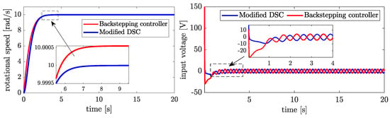
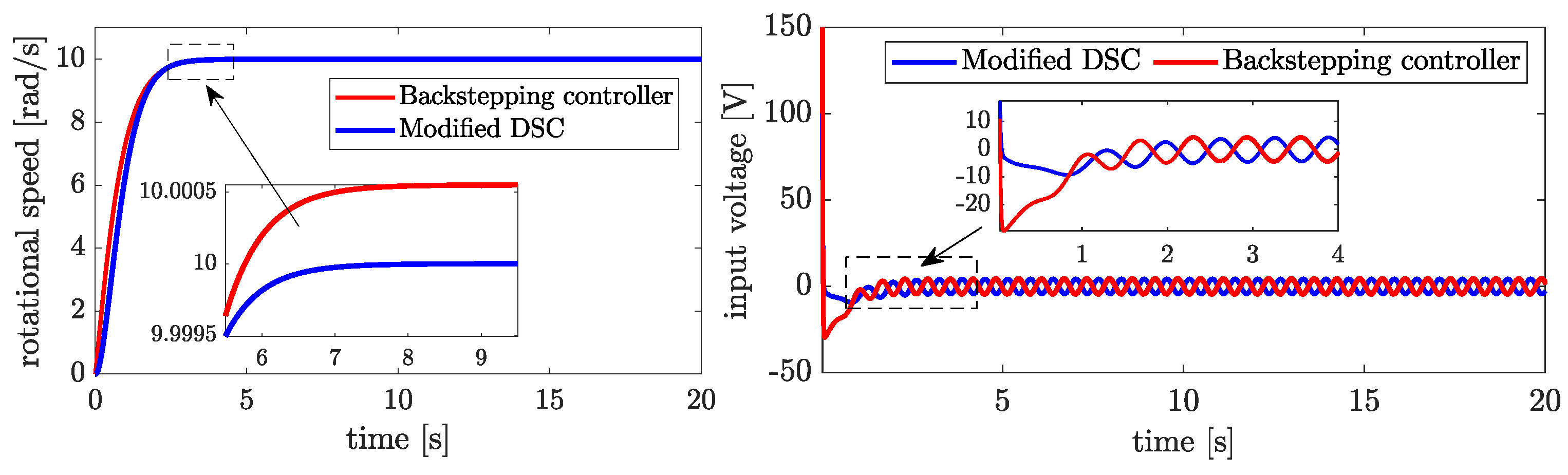
The response of the rotational speed and the input voltages with two controllers.
Figure 3.
Rotational speed response with different desired values.
Table 1.
Parameters of the 8/6 SRM [22].
- Scenario 1. Verifying the rotational speed stabilisation without external disturbances.
As mentioned above, this scenario aims to verify the control effectiveness in stabilising rotational speed without external disturbances. First, the traditional backstepping controller is given as [4]:
To ensure fairness and objectiveness, the controller parameters of two controllers are chosen as the same: , , , .
In Figure 2, a comparison between two controllers, the Backstepping controller and the Modified DSC, can be clearly observed through two graphs: the response of rotational speed and the input voltage signal. For the rotational speed , the Modified DSC demonstrates superior control as its response closely aligns with the target value of 10 rad/s without significant overshoot. This allows the system to reach a stable state without exceeding the desired value, ensuring high accuracy and minimizing steady-state error. In contrast, the Backstepping controller exhibits overshoot, with the rotational speed exceeding the target value before gradually stabilising. This slight oscillation can lead to undesirable fluctuations and increase the steady-state error in the control process.
Regarding the input voltage signal, the Modified DSC continues to show its advantages with a smoother control signal and fewer oscillations. The input voltage stabilises quickly with the Modified DSC and does not experience strong overshoot, which helps minimise unnecessary energy consumption and ensures system stability. Meanwhile, the Backstepping controller produces a more oscillatory input signal with noticeable overshoot, requiring more time for the system to achieve stability.
- Scenario 2. Verifying the rotational speed stabilisation with different desired values.
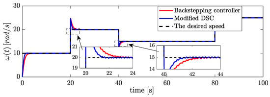
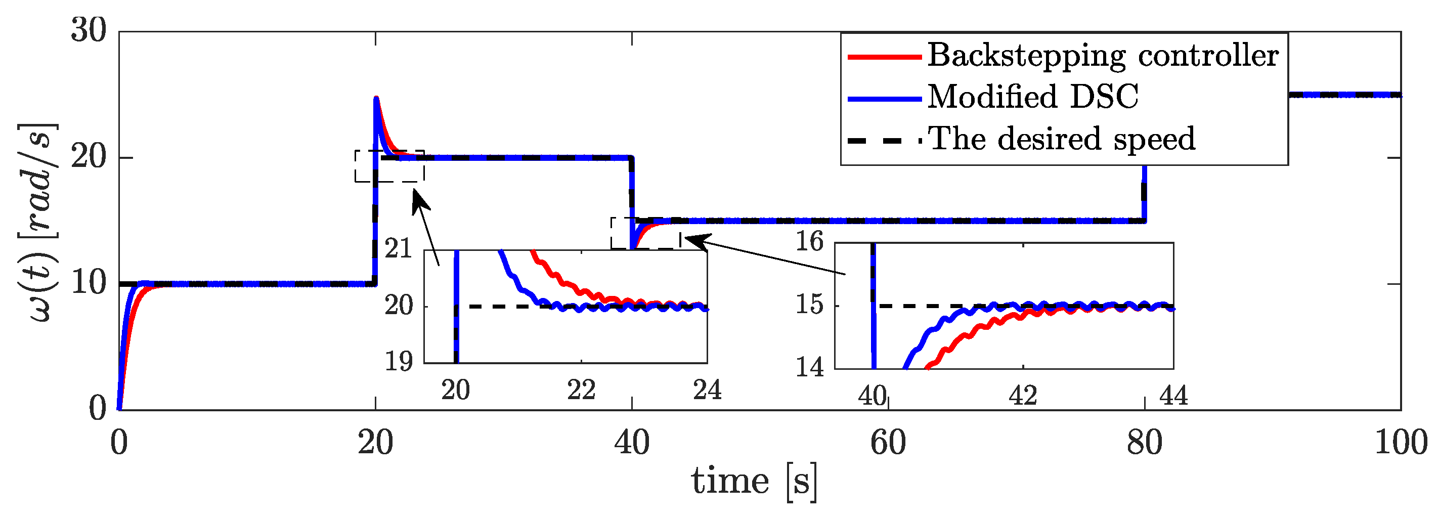
This section aims to verify the effectiveness of the proposed Modified DSC with different desired speeds. The values of are chosen as: within initial 20 s. from 20 s to 40 s. After 40 s, the desired speed is decreased at , and after 80 s, the desired speed is dramatically increased at .
Figure 3 illustrates a detailed comparison of the performance between two controllers: the Backstepping controller (represented by the red line) and the Modified DSC controller (represented by the blue line) in regulating the angular velocity over time. The black dashed line represents the desired speed, which acts as the target that both controllers aim to achieve. By analysing their responses across three key aspects—initial behaviour, transitional response, and steady-state performance—it becomes evident which controller performs better under varying conditions.
At the beginning, both controllers effectively increase the angular velocity from to the desired speed of approximately . During this phase, the system’s behaviour is stable, and neither controller produces significant oscillations, indicating that they are both well-configured for the initial rise. However, when the desired speed increases at , the performance differences between the two controllers become apparent. The Backstepping controller overshoots the new setpoint, reaching a peak angular velocity of around . In contrast, the Modified DSC controller overshoots less, peaking at approximately . Furthermore, the Modified DSC stabilises faster, exhibiting a smoother transition with fewer oscillations. This demonstrates that the Modified DSC controller is more efficient in handling sudden increases in the desired speed.
At , the desired speed decreases from back to . In this phase, the Backstepping controller again shows a noticeable overshoot, reaching approximately , and takes longer to settle into the new speed. Its response also includes some oscillations, suggesting less stability during this transition. In comparison, the Modified DSC controller continues to outperform by delivering a smoother and more precise response. It overshoots only slightly, reaching about , and quickly stabilises near the new desired speed. This ability to handle sudden decreases in the desired speed with minimal fluctuations highlights the Modified DSC’s better adaptability and superior dynamic response.
In the steady-state phase, when the desired speed remains constant, both controllers are able to maintain the desired speed with reasonable accuracy. However, the Modified DSC exhibits less oscillation and closer adherence to the setpoint. This demonstrates that the Modified DSC provides better stability and more precise tracking over longer durations, further solidifying its advantage.
5. Conclusions
In this paper, the modified dynamic surface control is proposed for strictly feedback nonlinear systems. It is shown that the Modified DSC method has the ability to improve the control performance of switched reluctance motors (SRMs). Including a sign function in the virtual control signal helps to fine-tune the accuracy and quickly reach a steady state without complicated steps. Simulation results demonstrate that the transient time is reduced and the response is better, especially when compared with traditional dynamic surface control methods. This is significantly meaningful in optimising the performance and durability of SRMs, especially in applications requiring high accuracy and energy efficiency.
Author Contributions
Conceptualization, D.M.D., T.V.T.C. and M.P.X.; methodology, T.V.T.C. and B.K.N.; software, D.M.D. and H.D.N.; validation, M.P.X. and T.V.T.C.; formal analysis, M.P.X.; investigation, M.P.X.; writing—original draft preparation, D.M.D.; writing—review and editing, D.M.D. and T.V.T.C.; visualization, B.K.N. and H.D.N.; supervision, M.P.X.; project administration, D.M.D. All authors have read and agreed to the published version of the manuscript.
Funding
This research received no external funding.
Institutional Review Board Statement
Not applicable.
Informed Consent Statement
Not applicable.
Data Availability Statement
The original contributions presented in this study are included in the article. Further inquiries can be directed to the corresponding author.
Conflicts of Interest
The authors declare no conflicts of interest.
References
- Rigatos, G.; Siano, P.; Ademi, S. Nonlinear H-infinity control for switched reluctance machines. Nonlinear Eng. 2019, 9, 14–27. [Google Scholar] [CrossRef] [Scilit]
- Nha, P.H.; Thuy, D.Q. Improving the characteristics of switched reluctance motor. Autom. Control Syst. Eng. J. 2016, 16, 59–66. [Google Scholar]
- Krishnan, R. Switched Reluctance Motor Drives: Modeling, Simulation, Analysis, Design, and Applications; CRC Press: Boca Raton, FL, USA, 2017. [Google Scholar]
- Hoang, N.P.; Van, H.P. Speed Control of switched reluctance motor using Adaptive Fuzzy Backstepping Sliding Mode Control. Int. J. Electr. Comput. Eng. Syst. 2024, 15, 459–467. [Google Scholar] [CrossRef] [Scilit]
- Chithrabhanu, A.; Vasudevan, K. Current sharing function based torque ripple reduction strategy for switched reluctance motor drives. In Proceedings of the 2021 IEEE 12th Energy Conversion Congress & Exposition-Asia (ECCE-Asia); IEEE: Piscataway, NJ, USA, 2021; pp. 2381–2386. [Google Scholar]
- Wong, K.; Cheng, K.W.E.; Ho, S.L. On-line instantaneous torque control of a switched reluctance motor based on co-energy control. IET Electr. Power Appl. 2009, 3, 257–264. [Google Scholar] [CrossRef] [Scilit]
- Cam, T.V.T.; Do Manh, D.; Le Xuan, H.; Duc, K.N.; Xuan, M.P. dynamic surface control for the switched reluctance motor. In Proceedings of the 2023 International Conference on System Science and Engineering (ICSSE); IEEE: Piscataway, NJ, USA, 2023; pp. 199–205. [Google Scholar]
- Vo Thi, C.T.; Manh Do, D.; Nguyen Duc, K.; Xuan Le, H.; Minh Phan, X. Stabilisation for multi-phase switched reluctance machine by a novel synchronisation of harmonic eradication mechanisms without resistance measurement and input-output relationships. Int. J. Control 2025, 98, 2021–2039. [Google Scholar] [CrossRef] [Scilit]
- Feng, L.; Sun, X.; Bramerdorfer, G.; Zhu, Z.; Cai, Y.; Diao, K.; Chen, L. A review on control techniques of switched reluctance motors for performance improvement. Renew. Sustain. Energy Rev. 2024, 199, 114454. [Google Scholar] [CrossRef] [Scilit]
- Asghar, K. Analysis of switched reluctance motor drives for Reduced torque ripple using FPGA based simulation Technique. Am. J. Inf. Sci. 2013. [Google Scholar]
- Tahour, A.; Meroufel, A.; Abid, H.; Aissaoui, A.G. Sliding controller of switched reluctance motor. Leonardo Electron. J. Pract. Technol. 2008, 12, 151–162. [Google Scholar]
- Rafiq, M.; Rehman, S.u.; Rehman, F.u.; Butt, Q.R.; Awan, I. A second order sliding mode control design of a switched reluctance motor using super twisting algorithm. Simul. Model. Pract. Theory 2012, 25, 106–117. [Google Scholar] [CrossRef] [Scilit]
- Islam, M.S.; Husain, I.; Veillette, R.J.; Batur, C. Design and performance analysis of sliding-mode observers for sensorless operation of switched reluctance motors. IEEE Trans. Control Syst. Technol. 2003, 11, 383–389. [Google Scholar] [CrossRef] [Scilit]
- Sun, J.; Cao, G.Z.; Huang, S.D.; Peng, Y.; He, J.; Qian, Q.Q. Sliding-mode-observer-based position estimation for sensorless control of the planar switched reluctance motor. IEEE Access 2019, 7, 61034–61045. [Google Scholar] [CrossRef] [Scilit]
- Carroll, J.J.; Geoghan, A.J.; Dawson, D.M.; Vedagarbha, P. A backstepping based computed torque controller for switched reluctance motors driving inertial loads. In Proceedings of International Conference on Control Applications; IEEE: Piscataway, NJ, USA, 1995; pp. 779–786. [Google Scholar]
- Wang, J. Speed-assigned position tracking control of SRM with adaptive backstepping control. IEEE/CAA J. Autom. Sin. 2016, 5, 1128–1135. [Google Scholar] [CrossRef] [Scilit]
- Alrifai, M.T.; Chow, J.H.; Torrey, D.A. Practical application of backstepping nonlinear current control to a switched-reluctance motor. In Proceedings of the 2000 American Control Conference; ACC (IEEE Cat. No. 00CH36334); IEEE: Piscataway, NJ, USA, 2000; Volume 1, pp. 594–599. [Google Scholar]
- Yang, Y.; Wen, Y.; Sun, X.; Wang, R. Overview of Fault-Tolerant Control for switched reluctance motor Drive Systems. J. Electr. Eng. Technol. 2025, 20, 5141–5164. [Google Scholar] [CrossRef] [Scilit]
- Sun, X.; Diao, K.; Lei, G.; Guo, Y.; Zhu, J. Study on segmented-rotor switched reluctance motors with different rotor pole numbers for BSG system of hybrid electric vehicles. IEEE Trans. Veh. Technol. 2019, 68, 5537–5547. [Google Scholar] [CrossRef] [Scilit]
- Izadian, A. Fundamentals of Modern Electric Circuit Analysis and Filter Synthesis; Springer: Berlin/Heidelberg, Germany, 2019. [Google Scholar]
- Khalil, H.K. Lyapunov stability. Control Syst. Robot. Autom. 2009, 12, 115. [Google Scholar]
- Ortega, R.; Sarr, A.; Bobtsov, A.; Bahri, I.; Diallo, D. Adaptive state observers for sensorless control of switched reluctance motors. Int. J. Robust Nonlinear Control 2019, 29, 990–1006. [Google Scholar] [CrossRef] [Scilit]

Disclaimer/Publisher’s Note: The statements, opinions and data contained in all publications are solely those of the individual author(s) and contributor(s) and not of MDPI and/or the editor(s). MDPI and/or the editor(s) disclaim responsibility for any injury to people or property resulting from any ideas, methods, instructions or products referred to in the content. |
© 2026 by the authors. Licensee MDPI, Basel, Switzerland. This article is an open access article distributed under the terms and conditions of the Creative Commons Attribution (CC BY) license.