Acoustic and Radio-Frequency UAV Detection: Classification Performance and Robustness Assessment in the Drodetect Project ^†

Abstract

The Drodetect project investigates unmanned aerial vehicle (UAV) detection using acoustic and radio-frequency (RF) signals. This study presents an independent experimental evaluation of both sensing modalities, analyzing their classification performance and sensitivity to synthetic perturbations. For the acoustic modality, 1182 windows from 15 recordings were analyzed using MFCC features and SVM classifiers, comparing original signals with those processed through spectral attenuation. The unfiltered model achieved an F1-score of 87.56%, while filtering increased false positives under perturbations, reaching a specificity of only 7.60% at $-5$ dB. For the RF modality, 1151 windows were evaluated using spectral features and SVM, with cross-day validation between acquisition dates. The results demonstrated strong discrimination between UAV-present and UAV-absent conditions, including under Gaussian perturbations applied to the spectral features, with balanced accuracy values of 89.84% and 90.43% at the highest evaluated perturbation level. Overall, the findings identify the strengths and limitations of both sensing modalities and provide an experimental foundation for their future integration through weighted decision-level fusion strategies.

1. Introduction

The use of unmanned aerial vehicles (UAVs) has expanded across various civilian applications, including precision agriculture, infrastructure inspection, environmental monitoring, and emergency response operations [1,2]. However, their increasing deployment also raises concerns regarding airspace security, privacy, and the protection of sensitive facilities [3]. These challenges have motivated research into systems capable of detecting and identifying UAVs, particularly in scenarios where their presence may pose a security risk [3].

The main technologies employed for UAV detection include radar, computer vision, radiofrequency (RF) signal analysis, and acoustic sensing [3]. RF-based systems analyze electromagnetic emissions associated with UAV communications, whereas acoustic systems exploit the sound signals generated during UAV operation [3,4]. Each modality exhibits distinct characteristics and limitations associated with the physical phenomena used to detect these platforms [3].

In RF-based UAV detection, Al-Sa’d et al. [5] investigated deep learning models for detecting and identifying UAVs through their electromagnetic emissions. Within this research area, Allahham et al. [6] documented the DroneRF dataset, which contains RF recordings from different drones under various operating conditions, as well as recordings collected in the absence of UAVs. These studies provide relevant foundations for developing and evaluating RF-based classification methods. Nevertheless, the characteristics of the electromagnetic environment and the presence of other transmission sources are important factors when assessing the performance of these systems [3].

Acoustic UAV detection, on the other hand, relies on analyzing sound signals generated by UAVs. Anwar et al. [7] investigated the extraction of cepstral features and the use of support vector machines to distinguish drone sounds, reporting favorable results under the experimental conditions considered. However, environmental noise, the distance between the UAV and the sensor, and the presence of other acoustic sources can affect detection performance [3]. Consequently, examining classifier behavior when signals exhibit conditions different from those encountered during training is important for understanding the limitations of acoustic detection methods.

Beyond individual approaches, previous research has explored the combined use of RF and acoustic information. Frid et al. [4] investigated machine learning and deep learning techniques for UAV classification, including a feature-fusion architecture based on recurrent neural networks. The authors evaluated model performance under different noise levels and reported favorable results for the combination of RF and acoustic features under certain conditions [4]. These findings highlight the relevance of both sensing modalities and the conditions under which detection systems are evaluated. In this context, experimentally examining their individual performance provides an opportunity to identify the specific strengths and limitations of each detection approach.

Against this background, the present study investigates UAV detection through the analysis of RF and acoustic signals collected during experimental acquisition campaigns using a coordinated recording initiation procedure. Signal processing and machine learning-based classification methods are independently evaluated for each modality, focusing on their ability to distinguish between UAV-present and UAV-absent conditions. Furthermore, classifier sensitivity to perturbations introduced during evaluation is investigated to characterize their behavior under the experimental conditions considered.

The main contributions of this work include the implementation of a coordinated RF and acoustic signal acquisition procedure, the experimental evaluation of classifiers for binary UAV detection, and the analysis of their sensitivity to signal perturbations. Additionally, the effect of a spectral filtering strategy on acoustic classification performance is examined, and limitations associated with distinguishing UAV-absent conditions are identified. Overall, this study provides experimental evidence regarding the performance and limitations of both detection approaches under the adopted evaluation protocols.

2. Data Collection and Feature Construction

2.1. Hardware Acquisition System and Environment

The experimental data acquisition platform consisted of two sensing subsystems designed to capture acoustic and radiofrequency (RF) signals associated with UAV operation. The acoustic subsystem employed a ReSpeaker USB 4-Mic Array (XVF3000 v3.0), equipped with four omnidirectional STMicroelectronics MP34DT01TR-M MEMS microphones, with a nominal sensitivity of $-26$ dBFS. The microphone array provided spatially distributed acoustic measurements for capturing sound signatures generated by UAV motors and propellers.

The RF subsystem consisted of a HackRF One software-defined radio (SDR), with a nominal operating frequency range of 1 MHz to 5.8 GHz. For the experimental acquisitions, the SDR was configured with a center frequency of 2.45 GHz and a sampling rate of 10 MS/s to capture RF activity in the 2.4 GHz band.

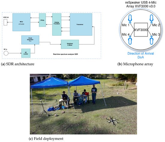
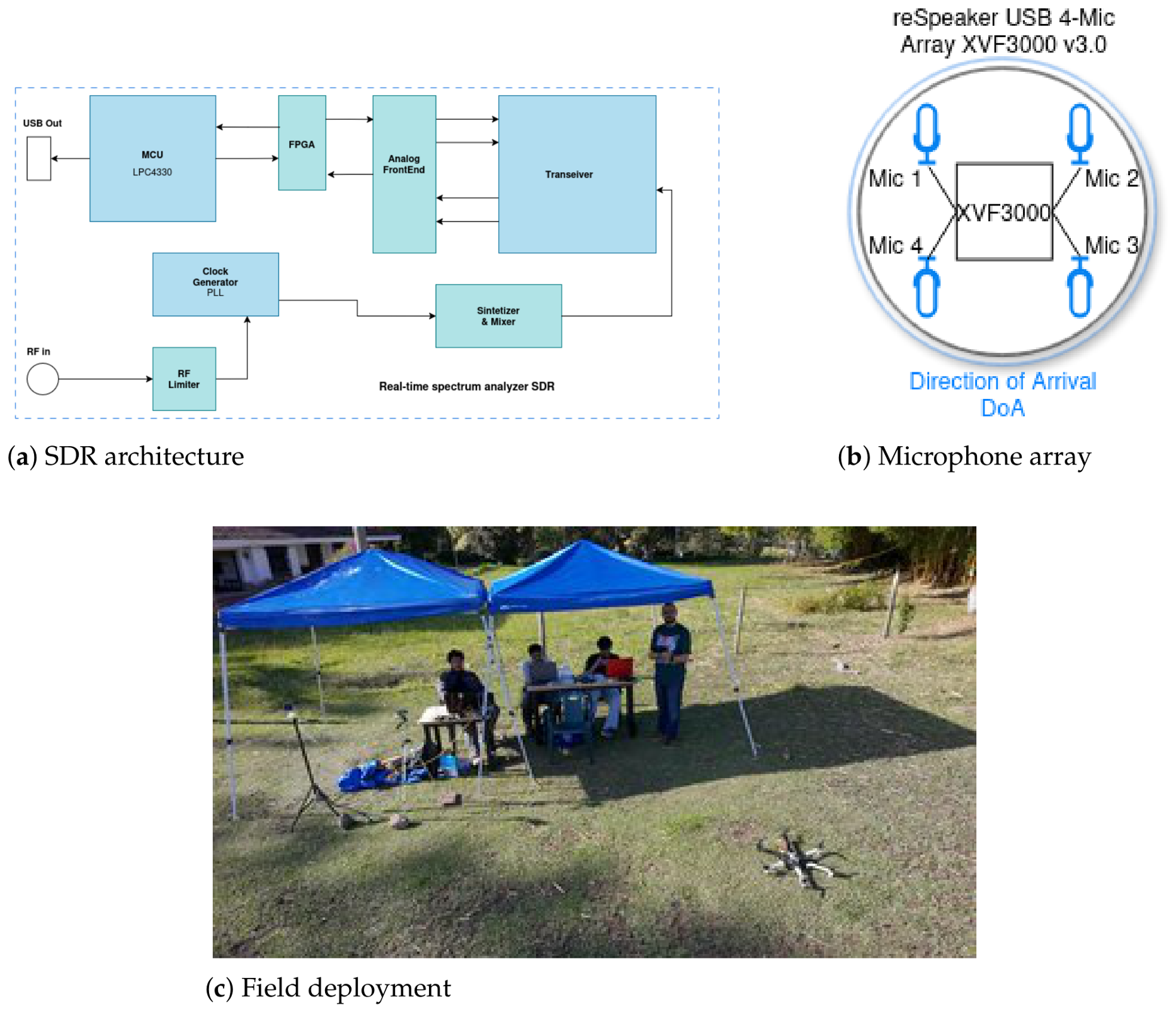
Both sensing devices were connected to a Linux-based laptop for data acquisition and storage. A coordinated recording procedure based on control flags was employed to initiate both acquisitions during the experimental sessions. Figure 1 illustrates the experimental setup, the microphone array configuration, and the functional architecture of the SDR receiver.

Figure 1. Experimental platform for RF and acoustic UAV signal acquisition: (a) functional architecture of the HackRF One SDR; (b) ReSpeaker USB four-microphone array configuration; and (c) field deployment of the acquisition system.

2.2. Mission Profile

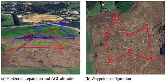
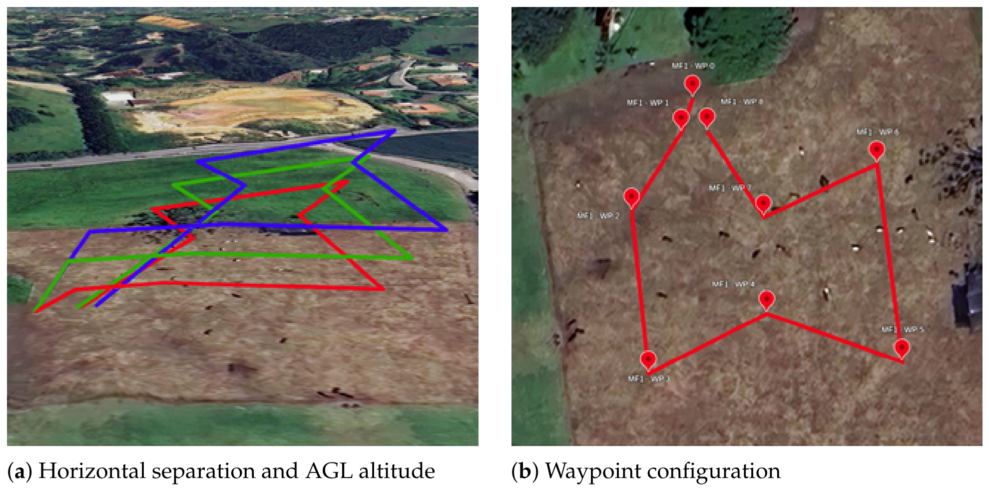
Three flight missions, designated MF1, MF2, and MF3, were designed to execute a similar flight profile under different conditions of horizontal separation and height above ground level (AGL). The objective was to maintain a consistent flight geometry across the three missions while introducing controlled variations in horizontal position and operating altitude, as illustrated in Figure 2a.

Figure 2. Flight profiles corresponding to the three missions (MF1: red, MF2: green, MF3: blue): (a) horizontal separation and AGL altitude; (b) waypoint configuration.

The horizontal separation between adjacent flight profiles was approximately 5 m. All three missions shared the same waypoint structure, although their absolute flight altitudes varied according to each mission’s configuration. The waypoint arrangement is illustrated in Figure 2b, while Table 1 summarizes the waypoint functions, reference AGL altitudes, and corresponding flight actions.

Table 1. Mission profile structure for the three missions.

Waypoint	Function	AGL (m)	Action
WP0	Takeoff	–	Take-off point and start of the mission
WP1	Waypoint	5	Start of route profile
WP2	Waypoint	10	Hold position for 2 s
WP3	Waypoint	10	Continuation of the trip
WP4	Loiter	15	Perform two turns within a 10 m radius
WP5	Waypoint	15	Continuation of the trip
WP6	Waypoint	10	Hold position for 2 s
WP7	Loiter	10	Perform two turns within a 5 m radius
WP8	Landing	–	Mission completion and landing

2.3. Dataset and Presence Labels

The updated dataset contains three hexarotor recordings, eight quadrotor recordings, and four unique negative recordings as we can see in Table 2. One exact negative PCM duplicate was excluded before splitting. Recordings are stereo 16-bit PCM at 44.1 kHz; only channel 0 is analyzed. No multichannel fusion or beamforming is performed on these exported files. Labels supplied by the experimenter apply to entire recordings, can be found at Github Repository. Its stronger initial audibility does not delimit presence. Physical presence may remain positive even when the acoustic contribution is weak.

Table 2. Updated dataset after exact-duplicate exclusion.

Class	Files	Duration (s)	Windows
Hexarotor	3	525.24	261
Quadrotor	8	1350.52	671
No UAV	4	502.50	250

Non-overlapping 2 s windows were extracted, discarding incomplete tails. The resulting 1182 windows comprise 932 positives and 250 negatives. The filenames span 31 August and 14 September 2026, but the folds are not date-disjoint. Windows from the same file are correlated and do not constitute independent sessions. This updated corpus differs from the earlier 10-recording pilot; their metrics are not directly attributable to a model improvement.

2.4. Common Acoustic Frontend

PCM samples are converted to floating-point amplitude without per-window peak normalization. The frontend uses 32 ms Hann frames (1411 samples), a 10 ms advance (441 samples), and a 2048-point FFT. Power is normalized by the squared-window sum. Sixty-four triangular HTK-Mel filters span 0–22.05 kHz and are individually normalized by their discrete sum. A ${10}^{-12}$ power floor precedes $10{\log }_{10}$ compression. An orthonormal type-II DCT produces 20 MFCCs; $C_0$ is discarded. Mean and population standard deviation of each remaining coefficient produce 38 features per window. Temporal pooling discards detailed trajectories. No pre-emphasis, resampling, or training augmentation is used. Direct log-Mel and PCEN classifiers have not been compared here.

2.5. Training-Negative Spectral Attenuation

For each negative training recording, power frames from 2 s excerpts starting every 4 s are pooled. Their median at each frequency forms a per-file profile; these profiles are averaged with equal file weights to obtain $N\left(f\right)$. Each fold uses three training-negative files; its held-out negative never contributes. Individual profiles may be precalculated, but only training identities are aggregated. For observed frame power $P(t,f)$, the simplified Wiener-inspired mask is

$$\begin{array}{cc}\hfill \widehat{S}(t,f)& =\max \left(P\right(t,f)-\alpha N(f),0),\hfill \end{array}$$

(1)

$$\begin{array}{cc}\hfill G(t,f)& =\max \left(g_{\min },{\displaystyle \frac{\widehat{S}(t,f)}{\widehat{S}(t,f)+\alpha N\left(f\right)+ϵ}}\right),\hfill \end{array}$$

(2)

$$\begin{array}{cc}\hfill \tilde{P}(t,f)& =G{(t,f)}^{2}P(t,f),\hfill \end{array}$$

(3)

with $\alpha =1$, $g_{\min }=0.20$, and $ϵ={10}^{-12}$. The floor limits amplitude attenuation to approximately 14 dB. The filtered power then passes through the same Mel/MFCC frontend. No waveform reconstruction is required. This is a heuristic mask, not an optimal Wiener estimator or proof of SNR improvement. Both classes receive identical processing.

2.6. RF Signal Processing

2.6.1. RF Dataset Preparation

The RF dataset was constructed from complex in-phase and quadrature (IQ) recordings acquired under UAV-present and UAV-absent conditions. The UAV-present class included quadrotor and hexarotor operations, whereas the UAV-absent class represented recordings collected without UAV activity.

The recordings were divided into non-overlapping 2 s windows, consistent with the temporal segmentation adopted for the acoustic modality. Each RF window was treated as an individual observation for spectral feature extraction and binary classification.

Duplicate observations were excluded before model evaluation to reduce the risk of identical windows appearing in different data partitions. Following the removal of 87 duplicate windows, the resulting dataset contained 1151 unique observations, comprising 865 UAV-present windows and 286 UAV-absent windows.

The recordings were collected during experimental sessions conducted on 31 August and 14 September 2026. The dataset was used to investigate the discrimination of UAV-related RF activity within the monitored frequency band.

2.6.2. Time-Frequency Representation

The complex IQ recordings were analyzed in the time-frequency domain using the short-time Fourier transform (STFT). For each 2 s observation, the STFT was computed using a Hann window of 4096 samples and an overlap of 2048 samples between consecutive frames.

The STFT of a discrete signal $x\left[n\right]$ can be expressed as

$$X(m,k)={\displaystyle \sum _{n=0}^{N-1}}x[n+mH]w\left[n\right]e^{-j2\pi kn/N},$$

(4)

where $N=4096$ is the analysis window length, $H=2048$ is the hop size, $w\left[n\right]$ is the Hann window, m represents the temporal frame, and k denotes the frequency bin.

The squared magnitude of the STFT was used to obtain a power-based spectral representation. This representation describes the distribution of received RF energy over time and frequency, allowing spectral activity associated with the monitored band to be examined.

The resulting spectrograms were represented using a resolution of 256 × 256 samples. This common representation facilitated the extraction of fixed-dimensional features from RF windows of equal duration.

2.6.3. Spectral Feature Extraction

Rather than using the complete spectrogram as input to the classifier, a compact spectral feature vector was obtained by averaging the power spectral density (PSD) representation along the temporal dimension.

For a spectrogram containing T temporal frames and F frequency bins, the resulting feature at frequency index k is defined as

$$\overline{P}\left(k\right)={\displaystyle \frac{1}{T}}{\displaystyle \sum _{m=1}^T}P(m,k),$$

(5)

where $P(m,k)$ denotes the spectral power at temporal frame m and frequency index k.

With $F=256$, each RF observation was represented by a 256-dimensional feature vector. This procedure retained information about the average spectral power distribution while reducing the dimensionality of the original time-frequency representation.

Temporal averaging also implies that detailed changes in spectral activity within each 2 s window are not explicitly preserved in the classifier input. Consequently, the resulting representation primarily characterizes the average frequency-dependent power distribution of each observation.

3. Classification and Evaluation

3.1. Acoustic Classification and Evaluation

Both pipelines use an RBF SVM with $C=1$ and gamma=scale. Standardization is fitted on training features only. Sample weights are proportional to $1/\left(G_c{n}_{g,c}\right)$, with $G_c$ training groups containing class c and $n_{g,c}$ windows in a group/class, and are normalized to unit mean. The decision threshold remains zero. SVM margins are not calibrated probabilities.

Four recording-disjoint folds are constructed by seeded permutation within each class followed by round-robin assignment (seed 42). Each fold holds out one negative and either two or three positives. Both pipelines use identical folds. There is no hyperparameter search or threshold tuning against the reported test labels. No independent-day or independent-session validation is claimed.

3.2. RF Classification and Evaluation

RF classification was evaluated independently from the acoustic classification pipelines. Each RF observation was represented by a 256-dimensional feature vector obtained by averaging the corresponding $256\times 256$ spectrogram along its temporal dimension.

Two support vector machine classifiers were evaluated: a linear SVM and a nonlinear SVM with a radial basis function (RBF) kernel. Both classifiers used a regularization parameter of $C=1$ and balanced class weights. For the RBF classifier, the kernel coefficient was set to gamma=scale.

Feature standardization was performed using a StandardScaler fitted exclusively on the training data. The same fitted transformation was subsequently applied to the corresponding test data.

RF classification followed a cross-day evaluation protocol using recordings acquired on 31 August and 14 September 2026. Two evaluation directions were considered: training on 31 August and testing on 14 September and vice versa. A separate classifier was trained for each direction.

To characterize sensitivity to perturbations in the extracted spectral features, zero-mean Gaussian noise was added to the test feature vectors. Six standard deviation levels were evaluated: 0, 0.5, 1, 2, 3, and 5, expressed in the units of the stored features.

For each level and evaluation direction, 30 repetitions were performed using reproducible random seeds. The training data, fitted scaler, and trained classifier remained unchanged during these repetitions.

Classification performance was quantified using accuracy, balanced accuracy, F1-score, and confusion matrices. The mean and standard deviation of the performance metrics were calculated across repetitions.

The perturbations were applied directly to the extracted feature vectors rather than to the original IQ recordings. Consequently, this analysis characterizes sensitivity to synthetic feature perturbations and does not constitute an evaluation under controlled physical RF interference or signal-to-noise ratio conditions.

RF and acoustic classification were evaluated independently. Multimodal feature-level and decision-level fusion were not implemented in the present study.

3.3. Metrics

UAV presence is positive. With rows denoting truth and columns prediction, the matrix is $[\mathrm{TN},\mathrm{FP};\mathrm{FN},\mathrm{TP}]$, corresponding to VN, FP, FN, and VP in the notebook. Metrics are

$$\begin{array}{cccc}\hfill \mathrm{Precision}& ={\displaystyle \frac{\mathrm{TP}}{\mathrm{TP}+\mathrm{FP}}},\hfill & \hfill \mathrm{Recall}& ={\displaystyle \frac{\mathrm{TP}}{\mathrm{TP}+\mathrm{FN}}},\hfill \end{array}$$

(6)

$$\begin{array}{cc}\hfill F_1& ={\displaystyle \frac{2\mathrm{TP}}{2\mathrm{TP}+\mathrm{FP}+\mathrm{FN}}},\hfill \end{array}$$

(7)

$$\begin{array}{cccc}\hfill \mathrm{Specificity}& ={\displaystyle \frac{\mathrm{TN}}{\mathrm{TN}+\mathrm{FP}}},\hfill & \hfill \mathrm{BA}& ={\displaystyle \frac{\mathrm{Recall}+\mathrm{Specificity}}{2}},\hfill \end{array}$$

(8)

$$\begin{array}{cc}\hfill \mathrm{Accuracy}& ={\displaystyle \frac{\mathrm{TP}+\mathrm{TN}}{\mathrm{TP}+\mathrm{TN}+\mathrm{FP}+\mathrm{FN}}}.\hfill \end{array}$$

(9)

Original-audio global metrics are computed from pooled held-out counts. They are window-level metrics, not event-level false alarms per hour. The always-positive reference is necessary because 78.85% of windows are positive.

For RF classification, accuracy, balanced accuracy, and F1-score were computed independently for each cross-day evaluation direction. Under synthetic feature perturbations, the mean and standard deviation of each metric were calculated across 30 repetitions at each perturbation level. RF results are also reported at the window level.

3.4. Five Testing-Only Perturbation Levels

Zero-mean white Gaussian noise is added to each held-out window at original-audio-to-added-noise power ratios of 20, 10, 5, 0, and $-5$ dB. For a unit-RMS noise realization z and original audio x,

$$x_L=x+z\sqrt{\left({\displaystyle \frac{1}{n}}\sum _{i=1}^n{x}_i^2\right){10}^{-L/10}}.$$

(10)

Because x already contains environmental noise, L is not the isolated UAV SNR. Three realizations per window use reproducible seeds derived from seed 20261006, file identity, start sample, and realization index. The same noise waveform is scaled across levels and supplied to both pipelines. Perturbations affect positives and negatives equally in procedure; labels remain physical-presence labels.

Models, scalers, and noise profiles remain frozen at their original-audio training values. No test-noise adaptation or retraining occurs. Floating-point mixtures are neither clipped nor renormalized, so this test does not simulate a saturating ADC. The five levels and three realizations yield 17,730 perturbed windows and 35,460 paired model predictions, not additional independent recordings. Gaussian noise does not reproduce wind, traffic, reverberation, or tonal interference.

3.5. RF Feature-Level Perturbations

To evaluate the sensitivity of the RF classifiers to variations in their input features, zero-mean Gaussian perturbations were added directly to the extracted 256-dimensional spectral feature vectors in the test partitions.

For an original feature vector f, the perturbed vector was defined as

$${\tilde{\mathbf{f}}}_{\sigma }=\mathbf{f}ϵ,ϵ\sim \mathcal{N}\left(\mathbf{0},{\sigma }^2\mathbf{I}\right),$$

(11)

where $\sigma$ denotes the standard deviation of the added perturbation in the units of the stored spectral features.

Six perturbation levels were considered: $\sigma \in \{0,0.5,1,2,3,5\}$. For each level and cross-day evaluation direction, 30 repetitions were performed using independent Gaussian noise realizations generated from reproducible random seeds.

Perturbations were applied exclusively to the test features. The training data, fitted standardization parameters, and trained SVM classifiers remained unchanged.

The same perturbation procedure was applied to the linear and RBF SVM classifiers, enabling a direct comparison of their sensitivity under equivalent test conditions.

Classification performance was summarized using the mean and standard deviation of accuracy, balanced accuracy, and F1-score across repetitions.

Unlike the acoustic perturbation experiment, the RF perturbations were not introduced into the original acquired signal. Therefore, the evaluated levels do not represent controlled RF signal-to-noise ratios or physical interference conditions.

4. Results

4.1. Original Audio: Filtering Did Not Improve the Baseline

Table 3 reports the updated corpus. Unfiltered MFCC–SVM achieved 88.67% precision, 86.48% recall, 87.56% F1, and 72.64% balanced accuracy. Filtering reduced these to 87.45%, 85.94%, 86.69%, and 69.97%, respectively. False positives increased from 103 to 115 and false negatives from 126 to 131. This configuration therefore did not improve the original-audio detector.

Table 3. Original audio: confusion counts and metrics (%). P: precision; R: recall; S: specificity; BA: balanced accuracy.

Measure	Unfiltered	Filtered	Always Positive
TN	147	135	0
FP	103	115	250
FN	126	131	0
TP	806	801	932
P (%)	88.67	87.45	78.85
R (%)	86.48	85.94	100.00
F1 (%)	87.56	86.69	88.17
S (%)	58.80	54.00	0.00
BA (%)	72.64	69.97	50.00

The always-positive reference obtains 88.17% F1, higher than both SVM variants, but zero specificity and 50% balanced accuracy. F1 alone thus cannot establish useful discrimination. Table 4 shows substantial fold variability, especially for negative rejection. No statistical significance is inferred from these four folds.

Table 4. Original-audio fold-level performance (%).

Fold	Model	F1	Specificity	BA
1	Unfiltered	90.91	3.70	51.66
1	Filtered	90.88	5.56	52.40
2	Unfiltered	75.78	74.55	69.40
2	Filtered	74.45	60.00	62.13
3	Unfiltered	94.05	86.96	89.36
3	Filtered	93.61	76.81	85.04
4	Unfiltered	87.29	61.11	77.25
4	Filtered	84.70	63.89	75.69

4.2. Robustness Under Added Gaussian Noise

Table 5 gives mean metrics over three noise realizations. The F1 standard deviation quantifies only randomness in generated noise, not uncertainty across independent field sessions. Table 6 reports mean confusion counts; fractional counts are averages, not counts from a single trial.

Table 5. Perturbed testing: mean percentages over three realizations; F1 shown as mean ± population standard deviation (percentage points). L is original-audio-to-added-noise power ratio. P: precision; R: recall; S: specificity; BA: balanced accuracy.

L (dB)	P	R	F1	S	BA
Unfiltered
20	80.27	83.08	$81.65\pm 0.07$	23.87	53.47
10	78.25	76.82	$77.53\pm 0.31$	20.40	48.61
5	77.87	74.00	$75.88\pm 0.03$	21.60	47.80
0	77.55	72.64	$75.01\pm 0.20$	21.60	47.12
−5	77.62	72.93	$75.20\pm 0.12$	21.60	47.26
Filtered
20	80.69	94.28	$86.95\pm 0.12$	15.87	55.07
10	79.50	92.81	$85.64\pm 0.09$	10.80	51.81
5	79.20	91.09	$84.73\pm 0.20$	10.80	50.95
0	79.00	89.99	$84.13\pm 0.06$	10.80	50.39
−5	79.16	94.13	$86.00\pm 0.03$	7.60	50.87

Table 6. Mean held-out confusion counts over three noise realizations; 1182 windows per realization.

L (dB)	TN	FP	FN	TP
Unfiltered
20	59.67	190.33	157.67	774.33
10	51.00	199.00	216.00	716.00
5	54.00	196.00	242.33	689.67
0	54.00	196.00	255.00	677.00
−5	54.00	196.00	252.33	679.67
Filtered
20	39.67	210.33	53.33	878.67
10	27.00	223.00	67.00	865.00
5	27.00	223.00	83.00	849.00
0	27.00	223.00	93.33	838.67
−5	19.00	231.00	54.67	877.33

At 20 dB, filtered recall increases to 94.28%, compared with 83.08% unfiltered, while filtered specificity drops to 15.87%, compared with 23.87% unfiltered. At $-5$ dB, filtered recall remains 94.13% and F1 is 86.00%, but specificity falls to 7.60%: on average 231 of 250 negative windows produce false detections. The corresponding unfiltered specificity is 21.60%, with 196 false positives. Thus, higher filtered recall and F1 under perturbation are accompanied by more false alarms rather than uniformly better discrimination.

Filtered balanced accuracy ranges from 55.07% at 20 dB to approximately 50–52% at the stronger perturbations; unfiltered balanced accuracy falls below 50% at 10 dB and below. The non-monotonic filtered recall between 0 and $-5$ dB should not be interpreted as recovery of the drone signal. A shift toward positive predictions is consistent with the accompanying loss of specificity, although its causal mechanism was not isolated.

4.3. Relationship to the Earlier Pilot

The previous pilot used ten different/partly overlapping recordings, 828 windows, and two folds. It yielded $(\mathrm{TN},\mathrm{FP},\mathrm{FN},\mathrm{TP})=(41,100,77,610)$ and 85.92% precision, 88.79% recall, 87.33% F1, and 29.08% specificity for MFCC–SVM. These historical results are retained for provenance, not as a matched comparison with the expanded corpus. Only the unfiltered and filtered pipelines within the current four-fold experiment isolate the effect of adding the mask.

4.4. RF Classification Results

The performance of the RF-based UAV detection approach was evaluated using a linear support vector machine (SVM) trained on spectral features extracted from the acquired RF signals. The dataset comprised 1151 two-second windows, including 865 UAV-present and 286 UAV-absent observations, after excluding a duplicated recording session. Each observation was represented by a 256-dimensional feature vector derived from its corresponding RF spectrogram.

A cross-day evaluation protocol was employed to assess classification performance across different acquisition dates. Two evaluation directions were considered: training on 31 August 2026 and testing on 14 September 2026 and vice versa. In both cases, training and testing observations were separated according to their acquisition dates.

4.4.1. Classification Performance Under Original RF Conditions

Under unperturbed conditions, the linear SVM achieved 100% accuracy, balanced accuracy, and F1-score in both evaluation directions. This indicates that all UAV-present and UAV-absent test windows were correctly classified, with no false positives or false negatives.

The balanced accuracy of 100% is particularly relevant because the dataset contained more UAV-present than UAV-absent observations. Therefore, the observed performance was not simply associated with the predominance of one class. Instead, the classifier correctly identified both conditions in the evaluated test partitions.

These results demonstrate that the extracted spectral features provided sufficient discriminative information to achieve complete separation between UAV-present and UAV-absent observations under the investigated experimental conditions. Furthermore, the classifier maintained the same performance when the training and testing dates were reversed, indicating that the discriminative information captured by the linear SVM remained effective across the two acquisition dates.

Nevertheless, the observed performance should be interpreted in relation to the field acquisition conditions. Although training and testing were conducted using recordings from different dates, the measurements belonged to a limited experimental campaign and employed the same RF acquisition hardware and measurement configuration.

The characteristics of the electromagnetic environment, background RF activity, and acquisition configuration may have contributed to the observed separation between the two classes. Consequently, the 100% classification performance demonstrates the effectiveness of the RF classification approach under the evaluated conditions, but does not necessarily imply equivalent performance in other electromagnetic environments.

4.4.2. Performance Under Synthetic Feature Perturbations

To characterize the sensitivity of the RF classifier to variations in its spectral input features, zero-mean Gaussian perturbations were introduced directly into the test feature vectors. Six perturbation levels were evaluated, corresponding to standard deviations of $\sigma \in \{0,0.5,1,2,3,5\}$, expressed in the units of the stored spectral features.

For each perturbation level and cross-day evaluation direction, 30 repetitions were performed using different reproducible noise realizations. The trained classifier and fitted standardization parameters remained unchanged throughout the experiments.

Table 7 summarizes the mean accuracy, balanced accuracy, and F1-score obtained for each perturbation level and evaluation direction.

Table 7. Performance of the linear SVM under synthetic Gaussian perturbations applied to RF spectral features. Values represent the mean across 30 repetitions and are expressed as percentages.

	Aug.–Sep.			Sep.–Aug.
$\mathbf{\sigma }$	Acc.	BA	F1	Acc.	BA	F1
0	100.00	100.00	100.00	100.00	100.00	100.00
0.5	100.00	100.00	100.00	100.00	100.00	100.00
1	99.97	99.98	99.98	100.00	100.00	100.00
2	99.78	99.37	99.88	99.76	99.66	99.61
3	99.03	96.99	99.45	98.14	97.80	96.98
5	95.13	89.84	97.21	90.72	90.43	85.66

The results show that the linear SVM maintained high classification performance as the magnitude of the synthetic perturbations increased. At $\sigma =0.5$, all evaluated metrics remained approximately equal to 100% in both evaluation directions. Similarly, at $\sigma =1$, balanced accuracy reached 99.98% when training on 31 August and testing on 14 September, while remaining at 100% in the reverse direction. These findings indicate that low-magnitude perturbations had a negligible effect on the classifier’s decisions under the evaluated conditions.

At $\sigma =2$, balanced accuracy decreased slightly to 99.37% and 99.66% for the two evaluation directions, respectively. Despite the introduction of classification errors, the model retained a high ability to discriminate between UAV-present and UAV-absent observations.

A more noticeable reduction was observed at $\sigma =3$, where balanced accuracy reached 96.99% and 97.80%, respectively. Nevertheless, both evaluation directions maintained balanced accuracy above 96%.

The largest performance reduction occurred at $\sigma =5$, the maximum perturbation level considered. Under this condition, balanced accuracy decreased to 89.84% when training on 31 August and testing on 14 September, and 90.43% in the reverse direction. Compared with the unperturbed condition, these values represent reductions of 10.16 and 9.57 percentage points, respectively.

Despite this decrease, balanced accuracy remained close to 90% in both evaluation directions, indicating that the classifier preserved substantial discriminative performance under the maximum evaluated synthetic perturbation.

4.4.3. Variability and Cross-Day Consistency

In addition to mean classification performance, the standard deviation across the 30 repetitions was analyzed to characterize the variability introduced by the different Gaussian noise realizations. At low perturbation levels, the standard deviations were close to zero, indicating highly consistent classification results across repetitions. As the perturbation magnitude increased, the variability became more pronounced.

At $\sigma =3$, the standard deviations of balanced accuracy were 0.93 and 0.99 percentage points for the August–September and September–August directions, respectively. At $\sigma =5$, these values increased to 1.86 and 1.78 percentage points, respectively. This behavior indicates that classification performance became more sensitive to the specific noise realization as the perturbation magnitude increased.

Despite the progressive reduction in classification performance, both evaluation directions exhibited similar balanced accuracy trends. At $\sigma =5$, balanced accuracy reached 89.84% and 90.43%, representing a difference of only 0.59 percentage points between the two evaluation directions.

These findings indicate that the linear SVM maintained comparable class-discrimination performance under synthetic feature perturbations, regardless of which acquisition date was used for training. However, the increasing standard deviation at higher perturbation levels shows that individual noise realizations had a greater influence on classification outcomes.

5. Limitations and Next Steps

Only four unique negative recordings support the current evaluation, and session/day independence is not established. Multiple windows and synthetic realizations remain correlated. Presence labels can exceed acoustic detectability at long range; elapsed time is not a measured distance. Existing clipping is not repaired by the spectral mask. A training-negative spectrum may also mismatch the test environment; the present experiment does not isolate this mechanism from model sensitivity to changed feature distributions.

The acoustic classification results also highlight the importance of addressing false-positive detections in UAV-free environments. Potential sources of acoustic interference include harmonic interferers and wind noise, although their individual contributions to the observed classification errors were not experimentally isolated. These factors should be considered when evaluating the acoustic detection approach under more challenging environmental conditions.

Next steps include additional independent negative sessions, realistic environmental perturbations, explicit day/session holdouts, and a controlled frontend comparison including log-Mel and PCEN. Per-channel energy normalization (PCEN), proposed for challenging far-field acoustic conditions, represents a relevant alternative to evaluate under the same recording-disjoint validation strategy. Filter strength and classifier thresholds require separate validation rather than retrospective tuning on these results. Robust training with augmentation is a distinct future experiment: the present augmentation is testing-only.

The RF evaluation presents different limitations. Although the linear SVM achieved 100% accuracy, balanced accuracy, and F1-score in both cross-day evaluation directions, the recordings were obtained during a limited experimental campaign using the same acquisition hardware and configuration. Consequently, the observed performance demonstrates the effectiveness of the classifier under the evaluated field conditions but does not establish equivalent generalization across different electromagnetic environments, acquisition locations, or propagation conditions. Furthermore, the possible influence of background RF activity and acquisition conditions on the observed class separation was not independently quantified.

The RF robustness experiments were conducted by introducing synthetic Gaussian perturbations directly into the extracted spectral feature vectors rather than into the original IQ recordings. Although balanced accuracy remained close to 90% at the maximum evaluated perturbation level, these results characterize the sensitivity of the classifier to feature-level perturbations and do not establish robustness against physical RF interference or controlled signal-to-noise ratio conditions. Additionally, the 30 repetitions performed at each perturbation level represent different synthetic noise realizations rather than independent acquisition sessions.

Future RF experiments should evaluate classification performance using recordings acquired in different electromagnetic environments, acquisition locations, and operating conditions. In particular, controlled interference experiments and perturbations applied directly to the original IQ signals would provide a more representative assessment of the classifier’s robustness against physical RF disturbances and changes in propagation conditions.

Both detection approaches should also be evaluated under more challenging real-world conditions, particularly in environments characterized by high levels of acoustic noise and electromagnetic interference. Such experiments would allow the sensitivity of each modality to environmental disturbances to be assessed and help identify the conditions under which classification performance deteriorates. Evaluating both approaches across different environmental conditions would also provide a more representative basis for assessing their potential complementarity.

Event-level false-alarm rates, synchronized flight-distance analysis, and audio–RF fusion remain unvalidated. Although both sensing modalities were independently evaluated, their combined detection performance has not yet been experimentally established. Future integration should investigate weighted decision-level fusion strategies, systematically evaluating the relative contribution of acoustic and RF classifiers to the final detection decision. The fusion weights should be determined through independent validation, considering classification performance, false-positive rates, and sensitivity to environmental disturbances. This analysis would help establish whether an appropriate combination of both modalities can improve UAV detection reliability compared with either modality operating independently.

6. Conclusions

On 15 unique recordings and 1182 windows, the unfiltered MFCC–SVM baseline outperformed the proposed soft attenuation mask on original audio. Under five levels of Gaussian test perturbation, filtering preserved higher recall and F1 but worsened negative rejection, reaching only 7.60% specificity at $-5$ dB. These results do not support claiming that filtering produced a reliable or generally noise-robust detector. They instead motivate improvements focused on false-positive control, broader environmental data, and independent-session validation before multimodal deployment.

For the RF modality, the linear SVM was evaluated using 1151 two-second windows represented by 256-dimensional spectral feature vectors. Under the original acquisition conditions, the classifier achieved 100% accuracy, balanced accuracy, and F1-score in both cross-day evaluation directions, correctly identifying all UAV-present and UAV-absent test windows. These findings demonstrate that the spectral representation enabled complete separation between the two classes under the investigated experimental conditions.

The RF classifier also maintained high classification performance under synthetic Gaussian perturbations applied to the test feature vectors. At the maximum evaluated perturbation level, balanced accuracy reached 89.84% and 90.43% for the two evaluation directions, respectively. These results indicate that the linear SVM preserved substantial discriminative capability despite increasing feature-level perturbations. Nevertheless, the observed performance should be interpreted within the evaluated acquisition conditions, since robustness against physical RF interference and generalization to different electromagnetic environments have not yet been established.

Overall, the results reveal different classification behaviors between the independently evaluated acoustic and RF modalities. While the acoustic approach exhibited limitations in negative-class rejection, the RF classifier achieved complete separation under the original experimental conditions and maintained high balanced accuracy under synthetic feature perturbations. These findings highlight the potential of RF-based classification while identifying specific improvements required for the acoustic detection approach. The independent evaluation of both modalities provides an experimental basis for future multimodal integration, although the potential benefits of combining their decisions remain to be established.

References

- Otto, A.; Agatz, N.; Campbell, J.; Golden, B.; Pesch, E. Optimization approaches for civil applications of unmanned aerial vehicles (UAVs) or aerial drones: A survey. Networks 2018, 72, 411–458. [Google Scholar] [CrossRef] [Scilit]
- Guebsi, R.; Mami, S.; Chokmani, K. Drones in precision agriculture: A comprehensive review of applications, technologies, and challenges. Drones 2024, 8, 686. [Google Scholar] [CrossRef] [Scilit]
- Seidaliyeva, U.; Ilipbayeva, L.; Taissariyeva, K.; Smailov, N.; Matson, E.T. Advances and challenges in drone detection and classification techniques: A state-of-the-art review. Sensors 2024, 24, 125. [Google Scholar] [CrossRef] [Scilit] [PubMed]
- Frid, A.; Ben-Shimol, Y.; Manor, E.; Greenberg, S. Drones detection using a fusion of RF and acoustic features and deep neural networks. Sensors 2024, 24, 2427. [Google Scholar] [CrossRef] [Scilit] [PubMed]
- Al-Sa’d, M.F.; Al-Ali, A.; Mohamed, A.; Khattab, T.; Erbad, A. RF-based drone detection and identification using deep learning approaches: An initiative towards a large open source drone database. Future Gener. Comput. Syst. 2019, 100, 86–97. [Google Scholar] [CrossRef] [Scilit]
- Allahham, M.S.; Al-Sa’d, M.F.; Al-Ali, A.; Mohamed, A.; Khattab, T.; Erbad, A. DroneRF dataset: A dataset of drones for RF-based detection, classification and identification. Data Brief 2019, 26, 104313. [Google Scholar] [CrossRef] [Scilit] [PubMed]
- Anwar, M.Z.; Kaleem, Z.; Jamalipour, A. Machine learning inspired sound-based amateur drone detection for public safety applications. IEEE Trans. Veh. Technol. 2019, 68, 2526–2534. [Google Scholar] [CrossRef] [Scilit]
Disclaimer/Publisher’s Note: The statements, opinions and data contained in all publications are solely those of the individual author(s) and contributor(s) and not of MDPI and/or the editor(s). MDPI and/or the editor(s) disclaim responsibility for any injury to people or property resulting from any ideas, methods, instructions or products referred to in the content. |
© 2026 by the authors. Licensee MDPI, Basel, Switzerland. This article is an open access article distributed under the terms and conditions of the Creative Commons Attribution (CC BY) license.