Robust Control Design and FEM-Based Validation for Oscillation Suppression in Second-Order Dynamic Systems ^†

Abstract

Vibration suppression of flexible robotic and industrial automation systems remains a critical challenge because structural flexibility, parameter uncertainties, and varying operating conditions can significantly degrade positioning accuracy, motion quality, and system reliability. This paper presents a robust control design framework for under-damped second-order dynamic systems with uncertain parameters, motivated by applications in robotic manipulators, servo-driven positioning platforms, and flexible industrial machinery. Three controller design approaches—compensation-based tuning, complete oscillation suppression, and optimal tuning based on a performance criterion—are analytically developed and comparatively evaluated. Closed-loop characteristic polynomials are derived for each method, and their robustness is investigated through pole-location and sensitivity analyses under variations of the damping ratio and system parameters. The proposed framework is further situated within the broader literature on real-time estimation and characterization of deformable, oscillatory, and vibrational systems. Representative approaches include extended Kalman filter-based maximum likelihood estimation for dynamic soft-tissue characterization, iterative and constrained Kalman-filter finite-element methods for soft-tissue modelling and deformation, reduced-order and adaptive unscented Kalman filters for online parameter identification, Hunt–Crossley contact-model estimation via radial-basis-function neural networks, and related nonlinear finite-element Kalman-filter techniques for real-time soft-tissue simulation. By relating the present sensor-fusion and disturbance-observer strategy to these established state-estimation methods, the work clarifies its methodological contribution to the robust control of uncertain flexible structures. To validate the methodology in a robotics-oriented context, a finite-element model (FEM) of a flexible cantilever beam representing a lightweight robotic link or flexible industrial structural component is developed and integrated with the control design procedure. MATLAB R2022b simulations are performed for a system with a natural frequency of 30 rad/s and damping-ratio variations from 0.05 to 0.15. The results indicate that conventional compensation and oscillation-suppression methods provide satisfactory nominal performance but exhibit significant pole migration and residual oscillations when parameter uncertainties are introduced. In contrast, the optimal tuning approach preserves stable pole locations and demonstrates substantially lower parametric sensitivity, leading to improved vibration attenuation and robust dynamic performance. The main contribution of this work is a combined analytical–numerical framework that links robust controller synthesis with FEM-based validation of flexible robotic and industrial structures under uncertainty, while embedding the design within the wider family of Kalman-filter and sensor-driven deformation-estimation techniques. The proposed approach provides a practical methodology for enhancing vibration control, positioning precision, and operational robustness in next-generation robotic systems and smart industrial automation applications.

1. Introduction

When choosing the desired location of the roots of the characteristic polynomial of a closed system, it must be taken into account that the real values of the parameters of the control object and the controller always differ from the calculated ones. If the conditions for the roughness of a closed system are met, then the question remains how the deviations of individual parameters affect the processes and their quality indicators in a real system. It is quite possible that setting a “good” desired location of the roots with parameter deviations can lead to worse quality indicators than those obtained by setting a different desired location of the roots, which takes into account in advance the possibility of parameter deviations from the calculated values [1,2,3,4,5,6].

As an example, here we can cite the problem of controlling an object with pronounced oscillatory properties when the parameters of the object, for one reason or another, may deviate from the calculated values. Attempts to obtain under these conditions in a closed system the aperiodic character of transient processes with the help of the corresponding desired arrangement of roots, for example, the binomial (p + ω₀)ⁿ, are unlikely to be successful. In a real closed system, fluctuations will inevitably occur. In this case, it may even turn out that the desired location with a more stable operation of a closed system, i.e., operation without abrupt changes in processes and their quality indicators, is set [7,8,9,10,11].

2. Formulation of the Problem

As a control object, we consider a second-order oscillatory system, which is under the influence of the control F and the perturbing forces F_B [12,13,14]:

$$m\ddot{y}+b\dot{y}+\mathit{cy}=F+F_B$$

(1)

where m is the mass; b is the coefficient of viscous friction; and c is hardness.

We bring Equation (1) to the standard form:

$$\ddot{y}+2\xi {\omega }_1\dot{y}+\omega \_1^2y=u+\phi$$

(2)

where ω₁ = $\sqrt{{\displaystyle \frac{c}{m}}}$ is the natural frequency; ξ = ${\displaystyle \frac{b}{2\sqrt{\mathit{cm}}}}$—dimensionless damping coefficient (ξ < 1); $u={\displaystyle \frac{F}{m}}$—control; and $\phi ={\displaystyle \frac{F_{\mathrm{B}}}{m}}$—perturbation.

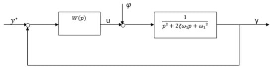
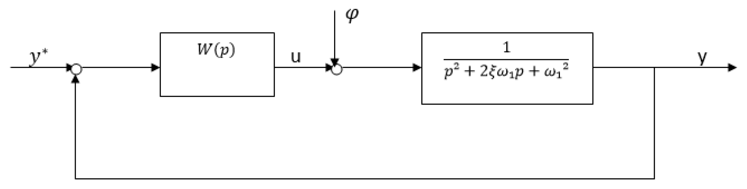
The block diagram of the control system for the problem of stabilizing system (2) is shown in Figure 1.

Figure 1. Block diagram of the control system.

In accordance with Equation (2), the calculated transfer function of the control object has the form

$$G(p)={\displaystyle \frac{1}{p^2+2{\mathit{\xi \omega }}_{1}p+{\omega }_1^2}}$$

(3)

We assume that the calculated value without the dimensional damping coefficient ξ is equal to the value ξ^*, while the actual value of the coefficient ξ in the object Equation (3) may differ from the calculated one. It is required to build a controller with a fixed setting, having a transfer function W(p) and providing for a closed system with the following:

• Effective vibration stabilization;
• Low sensitivity of the properties of a closed system to a change in the coefficient ξ.

3. Full Damping Method

Let us try to present a more stringent requirement to a closed system, namely the requirement of complete damping of oscillations at the natural frequency ω₁.

To do this, the expression 1 − H^d(p) must contain in the numerator the denominator of the transfer function of the object (3) [15,16,17]:

$$1-H^d(p)={\displaystyle \frac{(p^2+2\xi {\omega }_{1}p+{\omega }_1^2)(p+\gamma )p}{p^4+{{\alpha }_{1}p}^3+{\alpha }_2{p}^2+{\alpha }_{3}p+{\alpha }_4}}$$

(4)

The factor p in the numerator (4) ensures the fulfillment of the astatism condition H^d(0) = 1. The factor (p + γ) and the fourth order of the denominator are necessary to ensure the physical realizability of the controller. The coefficients of the characteristic polynomial α_i(i = $\overline{1,4}$) determine the desired location of the roots, for example, the binomial:

(p + ω₀)² = p² + 2ω₀p + ω₀²

(5)

From expression (4), it is easy to obtain the desired transfer function of the closed system:

$$H^d(p)={\displaystyle \frac{{\beta }_0{p}^2+{\beta }_{1}p+{\beta }_2}{p^4+{{\alpha }_{1}p}^3+{\alpha }_2{p}^2+{\alpha }_{3}p+{\alpha }_4}}$$

(6)

where β₀ = ${\alpha }_2-{\omega }_1^2-2\xi {\omega }_1\gamma$, β₁ = ${\alpha }_3-{\omega }_1^2\gamma$, β₂ = α₄, γ = α₁ − 2ξω₁.

Substituting expressions (3), (4) and (6) into the formula $W(p)={\displaystyle \frac{H^d}{\mathrm{G}\left[1-H^d\right]}}$, we get

$$W(p)={\displaystyle \frac{{\beta }_0{p}^2+{\beta }_{1}p+{\beta }_2}{(p+\gamma )p}}$$

(7)

The controller (7) does not directly compensate for the dynamics of the object (see Figure 1).

We write the differential equation of a closed system with a controller (7):

Q(s)y(t) = (β₀s² + β₁s + β₂)y^*(t) + (s + γ)sφ(t)

(8)

where Q(s) = s⁴+α₁s³ + α₂s² + α₃s + α₄—characteristic polynomial of a closed system at the calculated values of the parameters.

Thus, if the coefficients α_i(i = $\overline{1,4}$) are chosen, for example, in accordance with the binomial form of the fourth order,

$$Q(s)={(p+{\omega }_0)}^4=p^4+4{\omega }_0{p}^3+6{\omega }_0^2{p}^2+4{\omega }_0^{3}p+{\omega }_0^4$$

(9)

Then, for the calculated values of the parameters, all transient processes in the closed system (8) will be aperiodic.

It would seem that the goal has been achieved; however, the analysis of the characteristic polynomial of a closed system for small deviations of the object parameters from the calculated values is as follows:

$$\tilde{Q}(p)=(p^2+2\tilde{\xi }{\tilde{\omega }}_{1}p+{\tilde{\omega }}_1^2)(p+{\alpha }_1)p+{\beta }_0{p}^2+{\beta }_{1}p+{\beta }_2$$

(10)

This shows that oscillations are inevitable in a real system, and under certain conditions even loss of stability is possible.

For example, in the system (1) there was a slight change in the resistance forces, which led to the deviation $\xi =\tilde{\xi }-\xi$. In this case, the characteristic polynomial (10) is reduced to the form

$$\tilde{Q}(p)=p^4+({\omega }_1+2{\omega }_1∆\xi )p^3+\left[{\alpha }_2+2{\omega }_1∆\xi ({\alpha }_1-2\xi {\omega }_1)\right]p^2+{\alpha }_{3}p+{\alpha }_4$$

(11)

Naturally, the location of the roots of the real polynomial (11) will be different from the desired one. Let the binomial form (9) be chosen as the desired one. Then polynomial (11) can be rewritten in the following form:

$$\tilde{Q}(p)=p^4+2{\omega }_0(2+\sigma ∆\xi )p^3+2{\omega }_0^2\left[3+2\sigma ∆\xi (2-\sigma {\omega }_1)\right]p^2+4{\omega }_0^{3}p+{\omega }_0^4$$

(12)

where $\sigma ={\displaystyle \frac{{\omega }_1}{{\omega }_0}}.$

It can be seen from expression (12) that at large σ, regardless of the choice of an overestimated (∆ξ < 0) or underestimated (∆ξ > 0) value of the coefficient ξ as the calculated one for adjusting the controller, the necessary Stodola stability conditions may not be met. σ is possible with a high natural frequency ω₁ of the control object and a small value of the parameter ω₀, which in practice is always limited by the available control resource.

If we additionally consider the oscillatory stability limit of polynomial (12), which is obtained by equating to zero the penultimate Hurwitz determinant,

(2 + σ∆ξ)[10 + σ∆ξ(15 − 8σξ)] − 4 = 0

(13)

It turns out that instability at large σ is preceded by the appearance of oscillations in a closed system.

For small σ, the necessary and sufficient conditions for the stability of the polynomial (12) are satisfied. However, in this case, the nature of the transient processes will differ from the aperiodic one corresponding to the binomial form:

$$(p+{\mathit{\omega }}_0{)}^2=p^2+2{\mathit{\omega }}_{0}p+{\omega }_0^2$$

(14)

4. Results and Discussion

As a control object, we consider a second-order oscillatory system (2). We will assume that the dimensionless damping coefficient ξ, whose nominal value is equal to ξ^* (ξ^* < 1), can vary within certain limits. It is required to find the transfer function W(p) of the controller, which provides for the control-system, the block diagram of which is shown in Figure 1, low sensitivity with respect to small deviations of the parameter ξ of the control object from the nominal value ξ^*.

Let us first consider an auxiliary problem of optimal stabilization of a second-order oscillatory system with respect to the integral quadratic performance index of the type

$$J={\displaystyle {\int }_0^{\infty }}(x_1^T\mathit{Qx}+u^T\mathit{Ru})\mathit{dt}$$

(15)

This problem is necessary to justify the choice of weight matrices Q and R from (10).

Let us write the equation of the control object (2) at the nominal value of the parameter ξ = ξ^* in the state variables x₁ = y, $x_2=\dot{y}$:

$$\{\begin{array}{c}{\dot{x}}_1=x_2\\ {\dot{x}}_2=-{\omega }_1^2{x}_1-2{\xi }^{*}{\omega }_1{x}_2+u+\phi \end{array}$$

(16)

Optimality will be understood in the sense of the minimum of the integral of the weighted sum of the oscillation energy and the energy spent on control:

$$J={\int }_0^{\infty }({\omega }_1^2{x}_1^2+x_2^2+r{u}^2)\mathit{dt}$$

(17)

where the weighting factor r > 0 is not yet fixed.

The necessary condition for the extremum of the functional (17), which consists in the vanishing of its first variation, leads to the system of Euler–Lagrange equations:

$$\{\begin{array}{c}{\dot{x}}_1=x_2\\ \begin{array}{c}{\dot{x}}_2=-{\omega }_1^2{x}_1-2{\xi }^{*}{\omega }_1{x}_2+{\displaystyle \frac{1}{2r}}{\lambda }_2\\ {\dot{\lambda }}_1=2{\omega }_1^2{x}_1^2+{\omega }_1^2{\lambda }_2\end{array}\\ {\dot{\lambda }}_2=2x_2-{\lambda }_1+2{\xi }^{*}{\omega }_1{\lambda }_2\end{array}$$

(18)

We write the matrix A of system (18):

$$A=\left[\begin{array}{cccc}0& 1& 0& 0\\ -{\omega }_1^2& -2{\xi }^{*}{\omega }_1& 0& {\displaystyle \frac{1}{2r}}\\ 2{\omega }_1^2& 0& 0& {\omega }_1^2\\ 0& 2& -1& 2{\xi }^{*}{\omega }_1\end{array}\right]$$

(19)

and its characteristic equation:

$$\det [\mathsf{\nu }-A]=\det \left[\begin{array}{cccc}\nu & -1& 0& 0\\ {\omega }_1^2& \nu +2{\xi }^{*}{\omega }_1& 0& {\displaystyle \frac{-1}{2r}}\\ -2{\omega }_1^2& 0& \nu & -{\omega }_1^2\\ 0& -2& 1& \nu -2{\xi }^{*}{\omega }_1\end{array}\right]={\nu }^4+2B{\nu }^2+C=0$$

(20)

where B= ${\omega }_1^2(1-2{\xi }^{*})-{\displaystyle \frac{1}{2r}}$, $\mathrm{C}={\displaystyle \frac{{\omega }_1^2}{r}}+{\omega }_1^4>0$—coefficients depending on the parameters ξ^*and ω₁ of the control object.

Depending on the specific values of the parameters ξ^*, ω₁ and r, two cases are possible.

Case B² ≥ C. If in this case B > 0, then all the roots of the characteristic Equation (20) are purely imaginary, and there is no optimal stabilizing controller. In particular, it can be for a large value of r, which corresponds to a small control resource. If B < 0, then the roots of the characteristic Equation (20) have the form

ν_1,2 = ±γ₁, ν_3,4 = ±γ₂

(21)

where ${\gamma }_1=\sqrt{-B+\sqrt{B^2-C}}$, ${\gamma }_2=\sqrt{-B-\sqrt{B^2-C}}$

This case is typical for a small value of r, i.e., with a large control resource.

The solution of the system of Equation (18) with respect to the variable x₁ with real roots (4.8) is written as

$$x_1(t)=C_1{e}^{{\gamma }_{1}t}+C_2{e}^{{-\gamma }_{1}t}+C_3{e}^{{\gamma }_{2}t}+C_4{e}^{{-\gamma }_{2}t}$$

(22)

where C₁, C₂, C₃, and C₄ are arbitrary integration constants.

Free motion of a closed system for ξ = ξ^* aperiodic with characteristic equation is

(ν + γ₁)(ν + γ₂) = 0

(23)

For ξ ≠ ξ^*, the characteristic equation of a closed system has the form

ν² + [γ₁ + γ₂ + 2ω₁(ξ − ξ^*)]ν + γ₁γ₂ = 0

(24)

And when ξ < ξ^* the free movement of a closed system can become oscillatory; therefore, if the lower $\underset{¯}{\xi }\le \xi \le \overline{\xi }$ is defined, then the value ${\xi }^{*}=\underset{¯}{\xi }$ can be recommended as a nominal one, i.e., the smallest possible value.

With this setting, even with ξ = ξ^*, the free movement of a closed system

$$\ddot{y}+\left[2\gamma +2{\omega }_1(\xi -{\xi }^{*})\right]\dot{y}+({\gamma }^2+{\delta }^2)y=({\gamma }^2+{\delta }^2-{\omega }_1^2)y^{*}+\phi$$

(25)

will be oscillatory.

When carrying out numerical calculations, we use the following parameter values:

$${\omega }_1=30{\displaystyle \raisebox{1ex}{$1$}\!\left/ \!\raisebox{-1ex}{$s^2$}\right.}\cong 5\mathit{Hz};\hspace{1em}{\mathsf{\xi }}^{*}=0.1(0.05\le \mathsf{\xi }\le 0.15);r=1/{\omega }_1^2$$

(26)

For this data,

$$B=4321/s^2,\sqrt{C}=900\sqrt{2}1/s^2$$

(27)

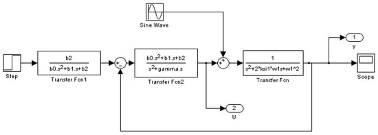
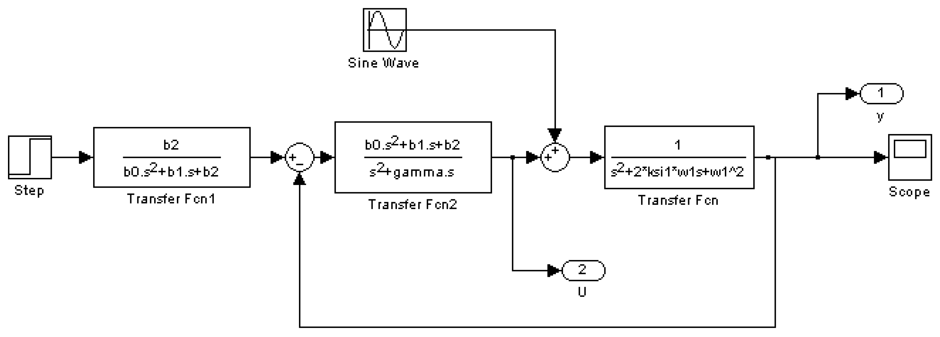
Let us return to the block diagram of the control system shown in Figure 2. Let us find the transfer function W(p) of a physically realizable controller of the minimum order, which provides for the closed system astatism of the first order and the desired characteristic polynomial (20). The solution is determined by the same formulas (6), (7) as in Section 3, in which the parameters α_i take the values ${\alpha }_i^{*}$ ($i=\overline{1,4}$).

Figure 2. Structural diagram of control with prefilter.

Recall that in Section 3 the controller (6) was tuned in accordance with the standard (binomial) form of the fourth order (8), and in the considered example, in accordance with the polynomial calculated by the criterion (18) minimizing not only the main motion (for ξ = ξ^*), but also for additional motion (for ξ ≠ ξ^*).

Note that in both cases it is expedient to introduce a prefilter with the transfer function into the control system:

$$L(p)={\displaystyle \frac{{\beta }_2}{{\beta }_0{p}^2+{\beta }_{1}p+{\beta }_2}}$$

(28)

excluding the influence of the numerator of the transfer function of the controller (7) on the indicators of the quality of transient processes. The corresponding block diagram is shown in Figure 2. In this case, the differential equation of the closed system will have the form

Q(s)y(t) = α₄y^* + (s + γ)sφ(t)

(29)

where $Q(s)=s^4+{{\alpha }_{1}s}^3+{{\alpha }_{2}s}^2+{\alpha }_{3}s+{\alpha }_4$ is a characteristic polynomial of a closed system.

Thus, for the control system, the block diagram of which is shown in Figure 2, three options for setting up a regulator with a gear ratio (7) are considered.

In all cases, the differential equation of a closed system has the same form (29). For different options for adjusting the controller, the following characteristic polynomials are obtained:

-

Adjustment according to the compensation method with the condition of complete damping of oscillations:

$$Q(s)=s^4+{{\alpha }_{1}s}^3+{{\alpha }_{2}s}^2+{\alpha }_{3}s+{\alpha }_4$$

(30)

Recall that the parameters ${\alpha }_i^{*}$ remained free, and it was recommended to use standard forms (binomial, Butterworth, etc.) to determine them.

Let us reduce the polynomials (30) to a common geometric mean root ${\omega }_0=\sqrt{{\omega }_1\sqrt{{\gamma }^2+{\delta }^2}}$ and find their roots with the above numerical data. In this case, we choose the binomial form as the standard one for the first two cases. The options for the location of the roots of the characteristic polynomial of a closed system are shown:

λ_1,2,3,4 = −ω₀ = −32.72 1/s

(31)

Let us present the main results of computer simulation below (Figure 3, Figure 4 and Figure 5):

With ξ^* = 0.15

Figure 3. Results of computer simulation with ξ^* = 0.15.

Figure 3. Results of computer simulation with ξ^* = 0.15.

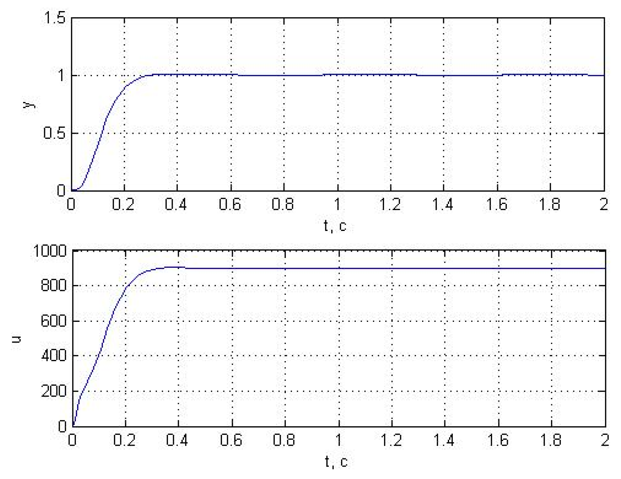
Transfer function:

1.146 × 10⁶

----------------------------------------------------

s⁴ + 133.9 s³ + 5682 s² + 2.524 × 10⁵ s + 1.146 × 10⁶

Roots:

−87.4380

−20.6153 + 45.8050i

−20.6153 − 45.8050i

−5.1924

With ξ^* = 0.1

Figure 4. Results of computer simulation with ξ^* = 0.1.

Figure 4. Results of computer simulation with ξ^* = 0.1.

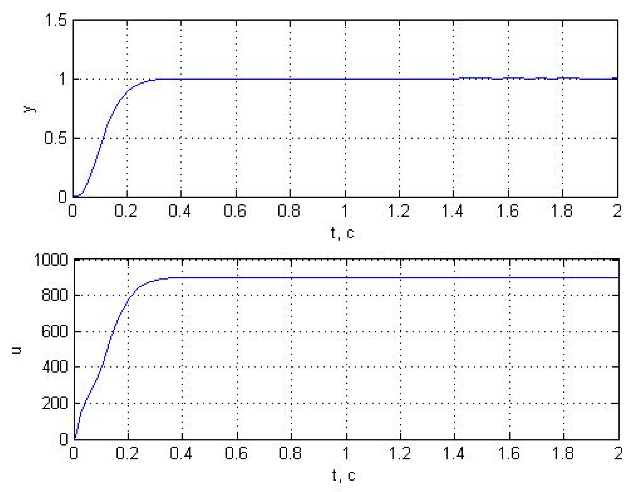
Transfer function:

1.146 × 10⁶

----------------------------------------------------

s⁴ + 130.9 s³ + 5679 s² + 2.524 × 10⁵ s + 1.146 × 10⁶

Roots:

−88.9421

−18.3879 +46.5416i

−18.3879 − 46.5416i

−5.1430

With ξ^∗ = 0.05

Figure 5. Results of computer simulation with ξ^* = 0.05.

Figure 5. Results of computer simulation with ξ^* = 0.05.

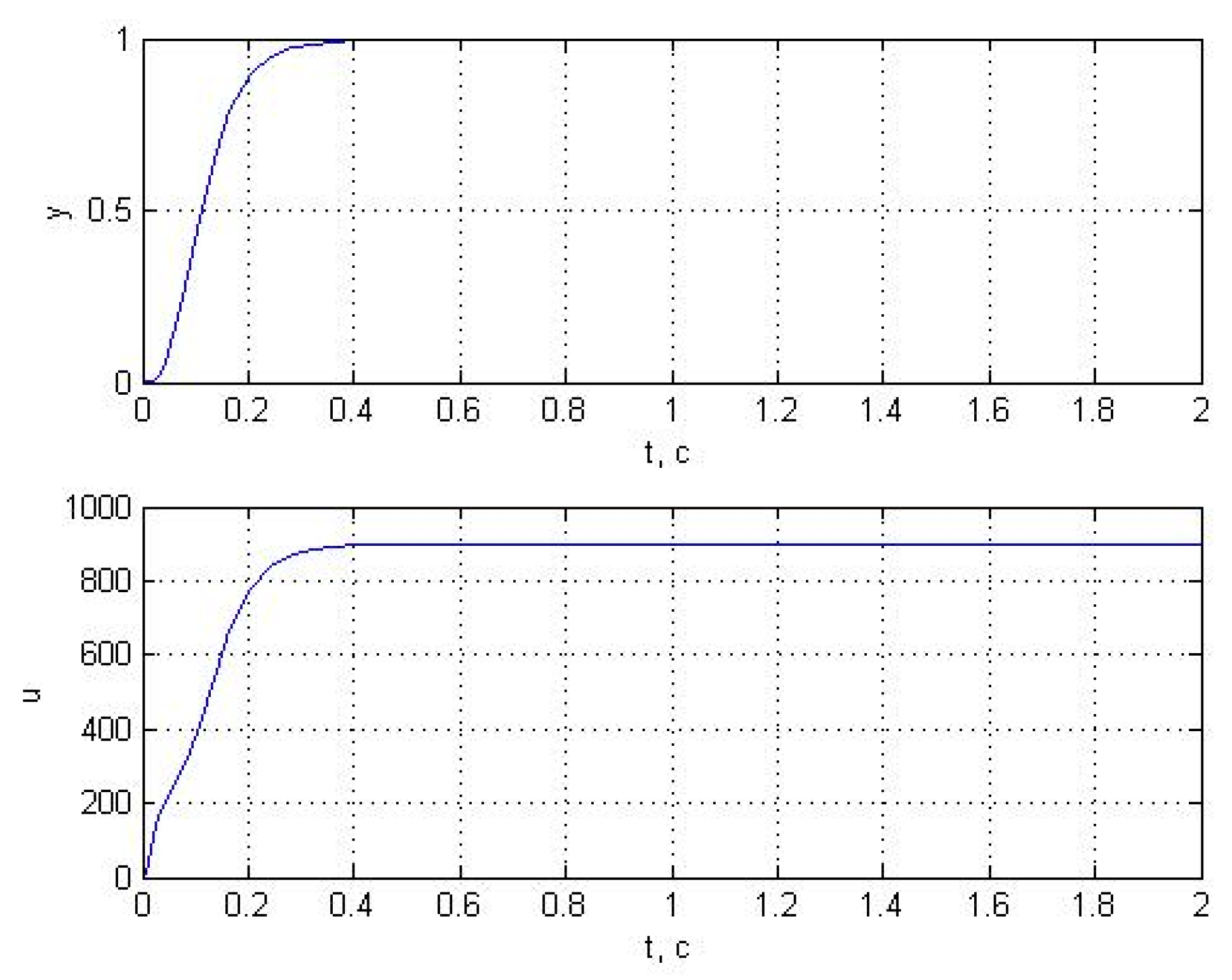
Transfer function:

1.146 × 10⁶

----------------------------------------------------

s⁴ + 127.9 s³ + 5676 s² + 2.524 × 10⁵ s + 1.146 × 10⁶

Roots:

−90.2954

−16.2350 + 47.1817i

−16.2350 − 47.1817i

−5.0955

A comparative analysis of the variants shows that the first variant has high parametric sensitivity, for which the characteristic polynomial (30) does not take into account the properties of the control object.

5. Conclusions

Thus, the optimal stabilizing control gives a quite acceptable result. The disadvantage in both cases is that the closed system does not have the property of astatism and the controller with the transfer function is not physically realizable.

In principle, control theory has methods to remove the noted shortcomings. Naturally, in this case, the quality indicators deteriorate somewhat compared to the optimal case considered above. Without going into the details about these methods, we recall that the goal of the first auxiliary problem was to choose the weight matrices Q and R from criterion (15).

References

- Pervozvanskii, A.A. Course in the Theory of Automatic Control; Nauka: Moscow, Russia, 1986. [Google Scholar]
- Dorf, R.C.; Bishop, R.H. Modern Control Systems; Laboratory of Basic Knowledge: Moscow, Russia, 2004. [Google Scholar]
- Preumont, A. Vibration Control of Active Structures: An Introduction, 3rd ed.; Springer: Berlin/Heidelberg, Germany, 2011. [Google Scholar]
- Gawronski, W.K. Advanced Structural Dynamics and Active Control of Structures; Springer: Berlin/Heidelberg, Germany, 2004. [Google Scholar]
- Bolton, W. Mechatronics: Electronic Control Systems in Mechanical and Electrical Engineering, 6th ed.; Pearson: London, UK, 2015. [Google Scholar]
- Alciatore, D.G.; Histand, M.B. Introduction to Mechatronics and Measurement Systems, 4th ed.; McGraw-Hill: New York, NY, USA, 2012. [Google Scholar]
- de Silva, C.W. Mechatronics: An Integrated Approach; CRC Press: Boca Raton, FL, USA, 2009. [Google Scholar]
- Fuller, C.R.; Elliott, S.J.; Nelson, P.A. Active Control of Vibration; Academic Press: Cambridge, MA, USA, 1996. [Google Scholar]
- Inman, D.J. Vibration with Control; John Wiley & Sons: Hoboken, NJ, USA, 2006. [Google Scholar]
- Jouaneh, M. Fundamentals of Mechatronics; Cengage Learning: Boston, MA, USA, 2012. [Google Scholar]
- Kuo, B.C.; Golnaraghi, F. Automatic Control Systems, 9th ed.; John Wiley & Sons: Hoboken, NJ, USA, 2010. [Google Scholar]
- Nise, N.S. Control Systems Engineering, 7th ed.; John Wiley & Sons: Hoboken, NJ, USA, 2015. [Google Scholar]
- Cetinkunt, S. Mechatronics; John Wiley & Sons: Hoboken, NJ, USA, 2007. [Google Scholar]
- Lyshevski, S.E. Electromechanical Systems and Devices; CRC Press: Boca Raton, FL, USA, 2008. [Google Scholar]
- Preumont, A. Vibration Control of Active Structures: An Introduction, 4th ed.; Springer: Berlin/Heidelberg, Germany, 2018. [Google Scholar]
- Bishop, R.H. (Ed.) The Mechatronics Handbook, 2nd ed.; CRC Press: Boca Raton, FL, USA, 2007. [Google Scholar]
- Onwubolu, G.C. Mechatronics: Principles and Applications; Elsevier Butterworth-Heinemann: Oxford, UK, 2005. [Google Scholar]
Disclaimer/Publisher’s Note: The statements, opinions and data contained in all publications are solely those of the individual author(s) and contributor(s) and not of MDPI and/or the editor(s). MDPI and/or the editor(s) disclaim responsibility for any injury to people or property resulting from any ideas, methods, instructions or products referred to in the content. |
© 2026 by the author. Licensee MDPI, Basel, Switzerland. This article is an open access article distributed under the terms and conditions of the Creative Commons Attribution (CC BY) license.