Synthetic-to-Real Transfer with a Causal Temporal Convolutional Network for Site-Calibrated Virtual Heat-Flux Sensing ^†

Abstract

This retrospective benchmark asks whether synthetic-only pretraining improves a causal temporal convolutional network (TCN) after 48 or 72 h of target-site heat-flow-meter (HFM) calibration. Six eligible public component records were evaluated over their complete chronological continuations with three optimization seeds. Four records met a prespecified normal-gradient heuristic; two low-gradient records were retained as defer stress tests. Pretrained and randomly initialized direct heat-flux TCNs used the same target calibration, architecture, and 10,000-epoch fitting protocol; a calibration-ratio continuation was the non-neural baseline. On normal-gradient cases, pretraining reduced mean heat-flux RMSE relative to site-only training by 8.4% at 48 h and 9.2% at 72 h, winning 12/12 and 11/12 paired seed/site comparisons. The result persisted after excluding the development site (9/9 at both durations). Pretraining also beat the ratio baseline in every normal-gradient comparison. However, it did not consistently improve HFM-integral U-value error, and low-gradient ratios were unstable. Thus, synthetic pretraining provided a small, consistent pointwise forecasting benefit within this limited corpus, but did not establish virtual replacement of HFM measurements or ISO 9869 procedures.

1. Introduction

In situ thermal transmittance is commonly assessed from heat-flux and temperature measurements. ISO 9869-1 specifies the heat-flow-meter (HFM) method for plane building components and remains current after confirmation in 2025 [1]. Its apparatus, installation, convergence, analysis, and reporting requirements cannot be replaced by applying an integral ratio to an arbitrary short record; duration and changing boundary conditions affect convergence [2,3].

A narrower operational problem arises when a survey has fewer HFMs than monitored locations. After a physical HFM calibrates one location, a causal virtual sensor could continue its heat-flux trace while the instrument is moved. Virtual HFM monitoring has been studied for existing envelopes [4], and earlier work by the present author trained an LSTM to predict heat flux from temperature difference [5]. A practical model must, however, adapt from little target data without using the future continuation.

This work therefore asks whether strictly synthetic-only pretraining can improve a direct, causal temporal convolutional network (TCN) after 48 or 72 h of target-site HFM calibration, compared with the same TCN trained only on that calibration and with a calibration-ratio baseline. The benchmark separates pointwise heat-flux forecasting from the integrated U-value implication. Its positive claim is deliberately bounded: transfer is evaluated at the series level on a small public corpus, not as replacement of an HFM or ISO 9869.

2. Materials and Methods

2.1. Public Records, Eligibility, and Quality Strata

The canonical public corpus contained 7 series and 9117 source rows from three versioned datasets [6,7,8]. Series 0 (second-floor wall) lasted 56.03 h and was ineligible because 48 h of calibration plus the required 12 h continuation needs at least 60 h. Series 1–6 were eligible at both durations: back wall, front wall, internal wall, roof, window, and Greenway hub. The internal-wall and window records had full-record mean $|∆T|\approx 1.38$ K, below the prespecified 3 K heuristic. They were labeled low-gradient/defer but retained as stress tests; the other four records formed the primary normal-gradient stratum. The heuristic is not a validated deployment threshold. Roof and Greenway are components, not additional walls.

All signals were placed on a 10 min grid. For each eligible series, the first 48 or 72 h was the target calibration and every subsequent sample was the complete chronological continuation. The full calibration was used for site fitting. Within each final benchmark fit, no continuation heat flux entered normalization, fitting, or checkpoint choice; final-epoch weights were used without continuation-based selection. The TCN and epoch count had already been fixed through the separately disclosed retrospective development analysis below, which used series 2. Seeds 42–44 were optimization repeats, not independent sites. The six records came from only two datasets, four normal-gradient records came from two datasets, and building-level independence was not established.

2.2. Exploratory Architecture Development

Before the final benchmark, one 72 h front-wall case (series 2) was used for a retrospective development comparison. Unlike the final benchmark, those models were pretrained with synthetic data and non-target public real records. Held-out milestones were reviewed retrospectively, so this experiment motivated fixing the TCN and 10,000 epochs but is neither unbiased model selection nor independent confirmation. At the fixed 10,000-epoch milestone, the direct TCN had the lowest RMSE among the four compared families (Table 1). This comparison does not isolate architecture causally because model development, protocol choices, and held-out milestone review were exploratory.

Table 1. Exploratory development comparison on series 2 after 72 h calibration (three seeds; mean ± sample SD). Pretraining included non-target public real records, unlike the synthetic-only final benchmark.

Direct Model	q RMSE (W/m2)	Notes at 10,000 Epochs
TCN	$0.6356\pm 0.0125$	$R^2=0.891$, Pearson $r=0.9499$
LSTM	$0.6973\pm 0.0410$	–
GRU	$0.6980\pm 0.0152$	–
Transformer [9]	$1.1688\pm 0.1132$	–

For the TCN at this milestone, integrated absolute heat-flux error was 34.93 Wh/m² and net cumulative error was $+9.43$ Wh/m². These diagnostics also showed that selecting a low pointwise RMSE does not guarantee an unbiased integral.

2.3. Reported Leakage-Controlled Transfer Benchmark

The final comparison used three models. ISOCalibrationRatio estimated a signed ratio only from the complete target calibration,

$$k_{cal}={\displaystyle \frac{{\sum }_{cal}q}{{\sum }_{cal}∆T}},{\widehat{q}}_{ratio}\left(t\right)=k_{cal}∆T\left(t\right).$$

(1)

This is an evaluation baseline, not the complete ISO 9869-1 procedure. SiteOnlyTCN began from random weights and used target calibration only, whereas PretrainedTCN began from the synthetic-only state described below and was adapted on the same calibration. Both predicted q directly and received no measured-q history, ratio/ISO prior input, residual blend, or post hoc bias correction.

At each time step the seven inputs were $∆T=T_{in}-T_{out}$, backward $d∆T/dt$, backward $d{T}_{in}/dt$, backward $d{T}_{out}/dt$, the difference between $∆T$ and its trailing 6 h mean, and 24 h sine/cosine elapsed-time features. Training used 12 h (72-step) windows with a 2 h stride. The TCN had a 96-unit input projection, five causal residual Conv1d blocks, kernel size 3, dilations 1, 2, 4, 8, and 16, and dropout 0.08. Its 63-step receptive field (10.5 h) fit within the 12 h window; the model had 140,737 parameters.

2.4. Synthetic-Only Pretraining and Site Adaptation

The corpus was generated with seed 42 by scripts/generate_synthetic.py. Using configs/synthetic_large.yaml, a two-node transient RC model produced 1200 HFM-style series from three- to five-layer stacks, six wall archetypes, and five weather profiles. Series lasted 144–288 h at 5, 10, or 15 min sampling; observed U was 0.123–2.436 W/(m²K). Randomized ranges were 17–24 °C indoor and $-10$–22 °C outdoor base temperature, 0–280 W/m² solar amplitude, 0.03–2.8 W/m² heat-flux noise SD, $-0.5$–0.5 W/m² bias, $-0.035$–0.035 W/m²/h drift, and 0.02–0.20 K temperature noise. Generated q combines dynamic wall, storage, solar, noise, bias, and drift effects; it is the label, not a measured public input.

The first 360 series by identifier were resampled to 10 min. For each seed (42–44), whole series were shuffled and split 70/15/15 into 252 training, 54 validation, and 54 held-out series; the latter were excluded from fitting and no synthetic-test result is reported. Feature and q z scores were fitted only on the 252 training series. With include_external_real: false, no public row entered pretraining or its normalization.

The seven inputs are listed above; q is target only. Twelve-hour windows (72 samples) used a 2 h stride, with deterministic without-replacement caps of 8192 training and 2048 validation windows per seed. One TCN was pretrained per seed using AdamW (learning rate $8\times {10}^{-4}$, weight decay $2\times {10}^{-5}$, batch 64), gradient-norm clipping at 1.0, and at most 260 epochs. The best normalized-q validation RMSE state was restored; stopping followed 60 epochs without improvement greater than $2\times {10}^{-5}$.

For a window w, let $z_i$ and ${\widehat{z}}_i$ be true and predicted normalized heat flux, let $q_i$ and ${\widehat{q}}_i$ be their physical-scale counterparts, and set $r_w={\sum }_{i\in w}{q}_i/{\sum }_{i\in w}∆T_i$ and ${\widehat{r}}_w={\sum }_{i\in w}{\widehat{q}}_i/{\sum }_{i\in w}∆T_i$. Pretraining uses

$${\mathcal{L}}_{pre}={\mathrm{mean}}_i{H}_1({\widehat{z}}_i-z_i)+0.01{\mathrm{mean}}_{w\in \mathcal{V}}S({\widehat{r}}_w-r_w)+0.02{\mathrm{mean}}_{i>1}{({\widehat{z}}_i-{\widehat{z}}_{i-1})}^2,$$

(2)

where $H_1$ is Huber loss ($\delta =1$), S is Smooth-L1, and $\mathcal{V}=\{w:|{\sum }_{i\in w}∆T_i|>{10}^{-4}\}$. The ratio target is derived from synthetic q, not independent U truth. The last term smooths normalized predicted q. Physics/prior-residual terms from the broader framework [10] evaluate to zero for this direct TCN, and the direct-U loss weight is zero.

The selected state was cached once per seed and cloned for every site and both durations: three pretraining runs, not one per case. Adaptation retained synthetic normalization and used all labeled target-calibration samples for exactly 10,000 epochs with AdamW ($3\times {10}^{-5}$ learning rate, $2\times {10}^{-5}$ weight decay, batch 32), clipping at 1.0, Huber/integral/smoothness weights 1/0.02/0.03, and final-epoch weights. SiteOnlyTCN used the same site protocol but random initialization and target-calibration normalization. No continuation q was used. The retrospective epoch choice remains potentially biased. The public repository https://git.hermeticum.io/Hermeticum/physics-informed-u-value (accessed on 29 October 2026) provides the fixed configuration configs/site_adaptation_all_public_tcn_transfer_48h_72h_mps_10k.yaml. The exact commands are

uv run python scripts/generate_synthetic.py \

  --config configs/synthetic_large.yaml

uv run python scripts/run_all_public_tcn_transfer.py --preflight

uv run python scripts/run_all_public_tcn_transfer.py --run

The reported run retained its exploratory label and is not prospectively confirmatory.

2.5. Metrics and Claim Units

Pointwise continuation metrics were q RMSE in W/m² and $R^2$. For cumulative diagnosis, HFM-integral U and model-integral U were

$$U_{HFM}=\left|{\displaystyle \frac{{\sum }_{test}q}{{\sum }_{test}∆T}}\right|,\widehat{U}=\left|{\displaystyle \frac{{\sum }_{test}\widehat{q}}{{\sum }_{test}∆T}}\right|.$$

(3)

The common 10 min interval cancels in these ratios. The U metric was $100|\widehat{U}-U_{HFM}|/U_{HFM}$. HFM-derived labels and $U_{HFM}$ are continuation references, not independent truth. Means and sample SDs summarize seed/site rows. Paired wins compare identical series and seeds. No inferential p-values are used because three seeds and a few physical records do not support such inference. Series 2 is included in the primary descriptive aggregate, while an explicitly non-development aggregate over series 1, 4, and 6 checks whether the pattern depends on that development case.

3. Results

3.1. Normal-Gradient Heat-Flux Forecasting

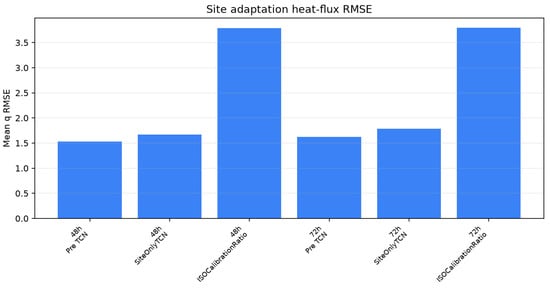
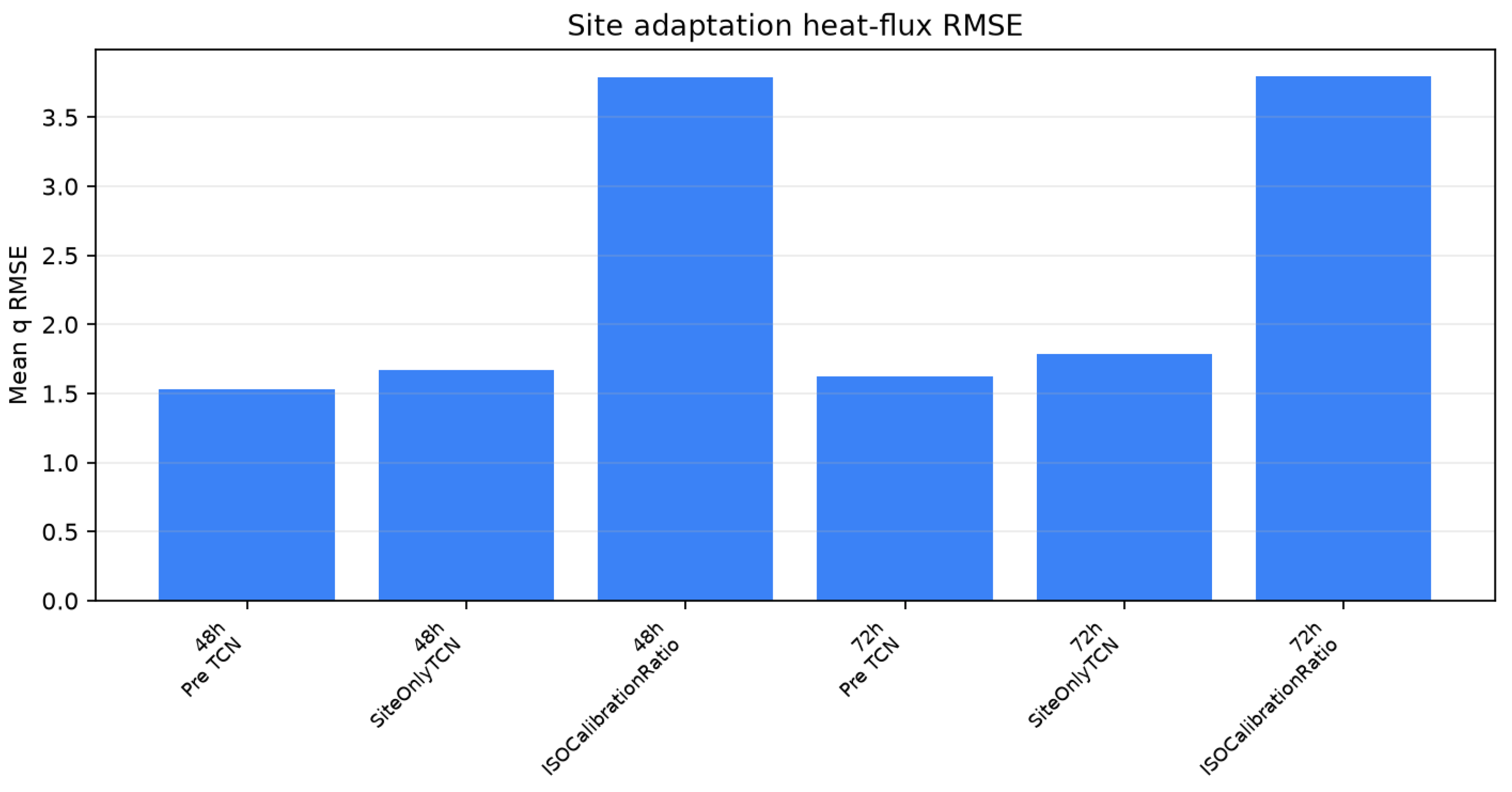
Table 2 and Figure 1 show the primary four-series aggregate. At 48 h, synthetic pretraining reduced mean q RMSE from 1.6716 to 1.5316 W/m² relative to site-only training (8.4%) and won all 12 paired seed/site comparisons. At 72 h, it reduced RMSE from 1.7885 to 1.6245 W/m² (9.2%) and won 11/12. It beat the ratio baseline in 12/12 comparisons at each duration, by 59.6% and 57.2% in aggregate. Extending calibration from 48 to 72 h did not lower aggregate q RMSE for any comparator.

Table 2. Normal-gradient continuation results over series 1, 2, 4, and 6 (12 seed/site rows per model and duration). RMSE is mean ± sample SD; U error is mean relative error against HFM-integral U.

Calibration	Model	q RMSE (W/m2)	Mean ${\mathit{R}}^2$	HFM-U Error (%)
48 h	Calibration ratio	$3.7920\pm 1.3442$	0.0104	9.9119
	SiteOnlyTCN	$1.6716\pm 1.2567$	0.8149	13.2614
	PretrainedTCN	$1.5316\pm 1.2329$	0.8401	17.5848
72 h	Calibration ratio	$3.7986\pm 1.2730$	0.0026	18.2181
	SiteOnlyTCN	$1.7885\pm 1.5237$	0.7525	23.4497
	PretrainedTCN	$1.6245\pm 1.3782$	0.7922	22.2438

Figure 1. Aggregate normal-gradient continuation q RMSE at 48 and 72 h. Bars summarize 12 seed/site rows per model and duration; seeds are optimization repeats, not independent sites.

The same ordering remained after excluding development series 2. At 48 h, mean RMSE was 4.4999, 2.0253, and 1.8536 W/m² for the ratio, site-only, and pretrained models; at 72 h it was 4.4785, 2.1488, and 1.9332 W/m². Pretraining won 9/9 comparisons against each comparator at each duration, reducing RMSE relative to site-only training by 8.5% and 10.0%. This is confirmatory only in the bounded sense that three non-development series reproduce the ordering; it does not supply independent buildings or nine independent sites.

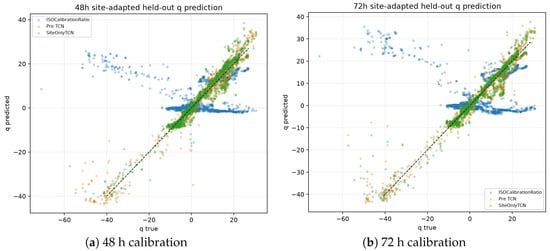
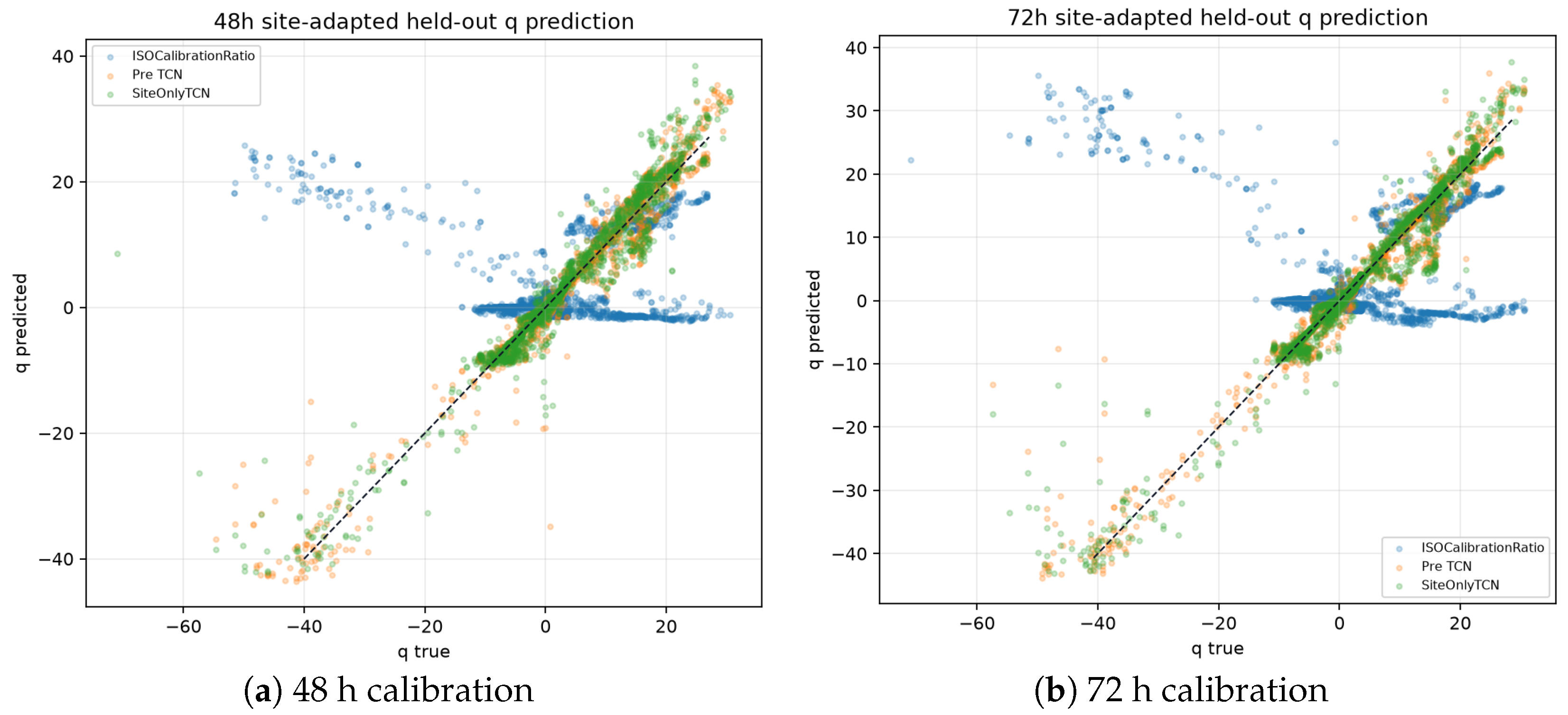
Per-site means further show that the benefit was not confined to the front wall. For back wall/front wall/roof/Greenway, pretrained versus site-only RMSE was 0.535/0.795, 0.566/0.611, 1.592/1.639, and 3.434/3.642 W/m² at 48 h. At 72 h the corresponding values were 0.416/0.554, 0.699/0.707, 1.610/1.693, and 3.774/4.199 W/m². Figure 2 displays the pooled pointwise relationship over all six eligible records using a reproducible random sample capped at 6000 trace rows per panel (seed 42), without treating samples as independent sites.

Figure 2. Predicted versus measured continuation heat flux for all six eligible records after (a) 48 h and (b) 72 h calibration, including the two low-gradient defer stress tests. Each panel is a random sample of at most 6000 exported trace rows using seed 42. Point density does not increase the number of independent physical cases.

3.2. Low-Gradient Stress Tests and Integrated U

Across all six eligible records, including the two defer cases, mean q RMSE at 48 h was 8.8946, 2.3133, and 2.2250 W/m² for the ratio, site-only, and pretrained models; at 72 h it was 9.9854, 2.3820, and 2.2647 W/m². Pretraining beat site-only training in 15/18 comparisons at each duration and the ratio in 18/18. These stress results support the robustness of pointwise q forecasting, but not deployment of a ratio-derived U estimate under weak excitation.

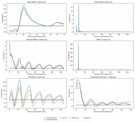
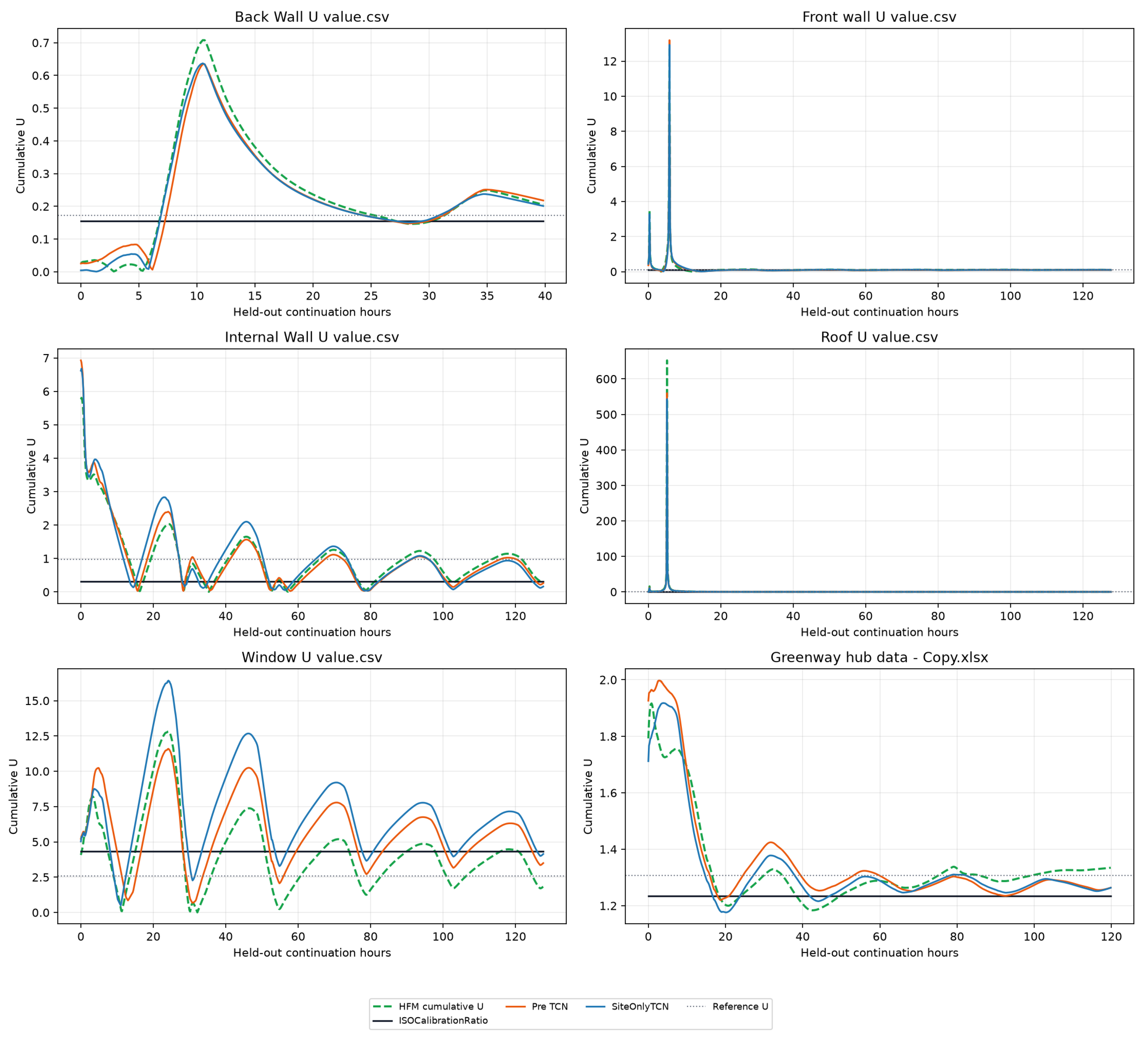
Improved q RMSE did not consistently improve the accumulated numerator in Equation (3). At 48 h, mean normal-gradient HFM-integral U error was 17.5848% for the pretrained TCN, 13.2614% for site-only training, and 9.9119% for the ratio. At 72 h, the corresponding errors were 22.2438%, 23.4497%, and 18.2181%. Excluding development series 2 gave 22.2255%, 16.8176%, and 12.0064% at 48 h, and 27.6546%, 27.8419%, and 20.4193% at 72 h. Pretraining therefore had no consistent integrated-U advantage despite its pointwise wins. Figure 3 shows all six 48 h cumulative traces: signed bias accumulates, while low-gradient denominator transients can produce large, unstable U excursions. The defer cases are not pooled into the primary U conclusion.

Figure 3. Six-case cumulative-U stress diagnostic after 48 h calibration. HFM q is used only for offline continuation evaluation. Internal-wall and window cases are low-gradient/defer stress tests; early denominator transients and unstable ratios are diagnostic, not deployable U estimates. Neural curves are arithmetic means over seeds 42–44 at each elapsed time; no seed-variability band is shown.

4. Discussion

Synthetic-only pretraining produced a small but unusually consistent pointwise benefit over random initialization: 23/24 normal-gradient paired wins across both durations, including 18/18 after removing the development site. The advantage is therefore not solely a replay of series-2 architecture development. Nevertheless, four normal-gradient records from two public datasets cannot establish transfer across buildings, climates, sensor installations, or component classes. The roof and Greenway results broaden component context but not the number of walls.

More calibration did not improve aggregate q forecasting from 48 to 72 h. This could reflect heterogeneous continuation regimes, fixed optimization, or the limited records; the benchmark does not identify a causal explanation. Likewise, the exploratory TCN/LSTM/GRU/Transformer ordering cannot support a general architecture claim because series 2, epochs, and protocol decisions were examined during development.

The integral result is the main deployment limitation. RMSE weights local squared errors, whereas U depends on signed cumulative q divided by cumulative $∆T$. Small persistent bias can therefore outweigh better pointwise tracking. Weak thermal gradients further condition the denominator, as the internal-wall and window stress tests demonstrate. A future reliability gate should prospectively check excitation, signed calibration bias, and block-integral agreement before allowing virtual continuation, and should defer rather than emit unstable U.

Other limitations include three seeds, only six eligible records, two source datasets, unestablished building independence, and heterogeneous supplied U references. Seeds measure optimization variability only. HFM-derived q labels and held-out HFM integration are references rather than independent truth. The final TCN and 10,000 epochs were fixed after retrospective development on series 2, so the benchmark is not free of development-selection bias even though its final continuations were excluded from fitting and checkpoint selection. No prospective relocation, uncertainty calibration, sensor-failure study, or validated quality threshold was performed.

5. Conclusions

After 48 or 72 h of target-site calibration, strict synthetic-only pretraining improved a causal direct-q TCN over the same randomly initialized TCN on the normal-gradient public cases. Mean q-RMSE reductions were 8.4% and 9.2%, with 12/12 and 11/12 paired wins; the ordering persisted on the three non-development cases. Pretraining also outperformed the calibration-ratio q baseline in every normal-gradient comparison. The gain was bounded to pointwise heat-flux forecasting: integrated U error did not improve consistently, and low-gradient U estimates were unstable and nondeployable. These retrospective results justify broader prospective transfer evaluation and reliability gating, but do not establish replacement of HFM measurements or ISO 9869 procedures.

References

- ISO 9869-1:2014; Thermal Insulation—Building Elements—In-Situ Measurement of Thermal Resistance and Thermal Transmittance—Part 1: Heat Flow Meter Method. International Organization for Standardization: Geneva, Switzerland, 2014.
- Choi, D.S.; Ko, M.J. Analysis of Convergence Characteristics of Average Method Regulated by ISO 9869-1 for Evaluating In Situ Thermal Resistance and Thermal Transmittance of Opaque Exterior Walls. Energies 2019, 12, 1989. [Google Scholar] [CrossRef] [Scilit]
- Alongi, A.; Sala, L.; Angelotti, A.; Mazzarella, L. In Situ Measurement of Wall Thermal Properties: Parametric Investigation of the Heat Flow Meter Methods through Virtual Experiments Data. Energies 2023, 16, 4247. [Google Scholar] [CrossRef] [Scilit]
- Jung, D.E.; Shin, D.H.; Seo, J.; Lee, K.H.; Kim, J. In-situ virtual heat flow meter model for monitoring heat flux of existing building envelope. Build. Environ. 2024, 253, 111320. [Google Scholar] [CrossRef] [Scilit]
- Gumbarević, S.; Milovanović, B.; Dalbelo Bašić, B.; Gaši, M. Combining Deep Learning and the Heat Flux Method for In-Situ Thermal-Transmittance Measurement Improvement. Energies 2022, 15, 5029. [Google Scholar] [CrossRef] [Scilit]
- Alkhatib, H.; Lemarchand, P.; Gavin, D.; Norton, B. A Study on U-Value Measurement for Energy Efficiency Enhancement. Dataset, Version 3. 2024. Available online: https://data.mendeley.com/datasets/xvhpnpnr3w/3 (accessed on 29 October 2026).
- Alkhatib, H.; Omar, O.; Norton, B. Long-Term Degradation of U-Values: A Dataset of Experimental Evidence and Energy Performance Consequences. Dataset, Version 1. 2025. Available online: https://data.mendeley.com/datasets/4kbb93bx32/1 (accessed on 29 October 2026).
- Alkhatib, H.; Norton, B. Façade Thermal Performance Dataset for Maintenance and Retrofit. Dataset, Version 1. 2026. Available online: https://data.mendeley.com/datasets/3gms2zvykb/1 (accessed on 29 October 2026).
- Vaswani, A.; Shazeer, N.; Parmar, N.; Uszkoreit, J.; Jones, L.; Gomez, A.N.; Kaiser, L.; Polosukhin, I. Attention Is All You Need. Adv. Neural Inf. Process. Syst. 2017, 30, 5998–6008. [Google Scholar]
- Raissi, M.; Perdikaris, P.; Karniadakis, G.E. Physics-informed neural networks: A deep learning framework for solving forward and inverse problems involving nonlinear partial differential equations. J. Comput. Phys. 2019, 378, 686–707. [Google Scholar] [CrossRef] [Scilit]
Disclaimer/Publisher’s Note: The statements, opinions and data contained in all publications are solely those of the individual author(s) and contributor(s) and not of MDPI and/or the editor(s). MDPI and/or the editor(s) disclaim responsibility for any injury to people or property resulting from any ideas, methods, instructions or products referred to in the content. |
© 2026 by the author. Licensee MDPI, Basel, Switzerland. This article is an open access article distributed under the terms and conditions of the Creative Commons Attribution (CC BY) license.