Mathematical Modelling and Analysis of the Thermal Characteristics of a Thermosiphon Solar Water Heating System ^†

Abstract

This article presents a mathematical model and analysis of the operating modes of a solar water-heating system with pump circulation. The aim of the study is to evaluate the daily dynamics of the system’s main thermal parameters based on calculated time-dependent values of solar radiation, ambient temperature, heat loss coefficient, useful heat flux, residual model error, and pump operating mode. The simulation results show that solar radiation intensity ranges from 0 to 860–880 W/m², with the active phase of solar exposure occurring approximately from 6:00 to 18:00, and maximum values being reached around midday. The ambient temperature varies between approximately 3 and 17 °C over the course of a day, while the heat loss coefficient ranges from 8.1 to 11.0 W/(m²·K). The system’s useful heat flux varies from 0 to 0.63–0.65 kW, reaching a maximum during the period of peak solar activity. It has been established that the system’s active heat output is primarily observed from 8:00 to 16:00. An analysis of the residual error between the calculated and measured temperature values showed that, in most cases, the deviations do not exceed approximately ±1.0 °C, which confirms the satisfactory adequacy of the developed model. Additionally, it is shown that the pump operates in a stable cyclic mode with binary states 0/1, ensuring periodic circulation of the coolant during the time interval under consideration. The results obtained confirm the feasibility of using the proposed model to predict the system’s energy efficiency, analyze pump control modes, and select optimal operating conditions for solar water-heating systems.

1. Introduction

Every year, renewable energy plays an increasingly significant role in our daily lives. The use of renewable energy sources helps reduce overall energy consumption and decrease dependence on fossil fuels. Solar energy is considered the most accessible and “direct” source of clean energy, as its use does not result in environmental pollution. Consequently, scientific research is actively developing mathematical models and engineering solutions for solar heating systems for domestic and residential buildings. A number of studies are devoted to evaluating the efficiency of solar hot water systems and their environmental impact. For example, in [1], a three-year data set collected in South Korea was used to analyze a solar hot water system for an apartment complex (14 buildings, 1179 families). It has been shown that, compared to a traditional water-heater (efficiency ≈ 85%), the solar system yields positive environmental benefits: fuel savings of approximately 71.9 L per year and a reduction in CO₂ emissions of approximately 186.3 tons. Study [2] presents a numerical simulation of a centralized solar HWS system designed for a high-rise residential building in Hong Kong. In [3], a system comprising a flat-plate collector, a storage tank, and a circulation loop was simulated; in addition, two heat transfer configurations (water–water and water–air) were compared, with the water–air configuration proving to be inefficient. The review [4] examines approaches to solar energy absorption in systems using various types of working fluids, with a primary focus on solar absorption refrigeration systems and related solutions (diffusion absorption, ejector-based, compression absorption, as well as cogeneration/trigeneration schemes). The thermodynamic properties of common working fluids, including ternary mixtures for solar absorption systems, were analyzed separately. The paper [5] presents an optical, thermal, and thermodynamic analysis of solar collectors and describes methods for evaluating their efficiency. The study [6] focuses on the design and energy efficiency of solar water-heating systems; the geometric parameters and dimensions of the system were selected based on the thermophysical properties of the materials. The paper [7] proposes calibration algorithms for small-scale solar hot water systems. Thermal performance is typically evaluated using the first law of thermodynamics (energy balance); however, this is insufficient for a comprehensive analysis of a flat-plate solar collector [8]. Applying the second law of thermodynamics (the exergetic approach) allows for accounting for various types of losses in the collector and provides a more accurate assessment of the solar HWS system as a whole [9,10,11].

The purpose of this work is to develop a mathematical model of a solar water-heating system with pump circulation and to conduct a numerical analysis of its operating modes in order to evaluate its thermal performance, heat losses, the quality of heat carrier circulation control, and the adequacy of the model based on the comparison of calculated and measured data.

2. Methodology: Mathematical Modelling

The thermal state of the absorber plate is described by a non-stationary energy balance equation that accounts for the influx of useful solar energy and heat losses/transfer to the heat carrier and the environment:

$$C_p{\displaystyle \frac{d{T}_p}{\mathit{dt}}}=A\hspace{0.17em}{\eta }_{\mathit{opt}}\hspace{0.17em}I\left(t\right)-h_{\mathit{pf}}A\hspace{0.17em}\left(T_p-T_f\right)-U_{b}A\hspace{0.17em}\left(T_p-T_a\right)-U_{t}A\hspace{0.17em}\left(T_p-T_a\right),$$

(1)

where m—absorber weight, kg; c_p—specific heat capacity of the plate material, J/(kg·K); T_p(t) —plate temperature, °C or K; A—effective aperture area of the collector, m²; I(t)—solar radiation on the collector surface, W/m²; η_opt—optical efficiency (transmission through glass × absorption), dimensionless.

Here, the first term on the right-hand side represents the fraction of incident solar radiation absorbed by the plate, taking into account optical losses; the second term describes the transfer of heat from the plate to the heat carrier through channels/tubes (convective “plate–fluid” coupling), and the last two terms correspond to the heat losses through the rear insulation and through the top cover (glass), respectively.

Usually:

η_opt = τ_gα_p (or (τα)_eff),

(2)

h_pf —heat transfer coefficient “plate → heat carrier”, W/(m²·K); A_pf —area of thermal contact “plate–channels/tubes, m²; U_b—the calculated heat loss coefficient through the rear wall, W/(m²·K); A_b —the area of the rear surface (usually A_b ≈ A); U_t—the calculated heat loss coefficient through the roof (glass + convection/radiation), W/(m²·K); A_t—upper surface area (usually A_t ≈ A); T_f(t)—average temperature of the heat carrier in the absorber/channels, °C or K; T_a(t)—ambient air temperature, °C or K.

The dynamics of the average heat carrier temperature in the absorber/channel zone are described by a non-stationary heat balance equation that accounts for heat exchange with the absorber plate and convective energy transfer due to fluid flow:

$$C_f{\displaystyle \frac{d{T}_f}{\mathit{dt}}}=h_{\mathit{pf}}A\hspace{0.17em}\left(T_p-T_f\right)+\dot{m}{c}_p\left(T_{\mathit{in}}-T_f\right),$$

(3)

here T_in—return temperature from the tank heat exchanger (equivalent to T₁ in our article, which is included in the baseline—via inflow/outflow).

The first term on the right-hand side corresponds to the heat flow to the coolant from the plate through the heat transfer coefficient h_pf. The second term describes the energy exchange due to mass flow: the coolant enters the collector at temperature T_in, and the flow exits the mixing zone at average temperature T_f. The temperature T_in corresponds to the temperature of the return pipeline after the tank heat exchanger (equivalent to the variable T₁ the base model), and it is this temperature that defines the “initial” state for the heat carrier’s ODE via the flow rate $\dot{m}$.

The thermal state of the glass coating is described by the non-stationary energy balance equation, in which the glass receives heat from the absorber through the air gap and loses it to the environment via convection (wind) and radiation:

$$C_g{\displaystyle \frac{d{T}_g}{\mathit{dt}}}=h_{\mathit{pg}}A\hspace{0.17em}\left(T_p-T_g\right)-\left(h_w+h_{r,g-a}\right)A\hspace{0.17em}\left(T_g-T_a\right),$$

(4)

where T_g(t) is the glass (coating) temperature, K or °C; T_p(t) is the absorber (plate) temperature, K or °C; T_a(t) is the ambient air temperature, K or °C; t is time, s; and C_g is the lumped heat capacity of the glass, J/K.

In this study, the top heat losses of a flat-plate collector are specified using the reduced heat loss coefficient U_t, which is determined by the total thermal resistance of heat transfer in the “absorber–glass” air gap and at the outer surface of the “glass–ambient” interface. In this case, the convective and radiative components of heat transfer are considered together, and the top heat loss coefficient is calculated using the expression

$$U_t={\left({\displaystyle \frac{1}{h_{c,p-c}+h_{r,p-c}}}+{\displaystyle \frac{1}{h_w+h_{r,c-a}}}\right)}^{-1}.$$

(5)

The radiative heat transfer coefficients h_r,p−c and h_r,c−a, as well as their relationship to the glass temperature, are calculated using an iterative procedure, since radiative heat transfer depends on the current surface temperatures.

In the proposed model, the coefficients are calculated dynamically; that is, at each simulation step, h_c,p−c(t), h_r,p−c(t) and h_r,c−a(t) are updated based on the current temperature values. The convective coefficient in the gap h_c,p−c(t) is determined using natural convection correlations based on similarity criteria:

$$\mathit{Nu}\left(\mathit{Ra},\mathit{Pr}\right)={\displaystyle \frac{h_{c,p-c}L}{k}},\mathit{Ra}={\displaystyle \frac{\mathit{g\beta }\Delta T\hspace{0.17em}{L}^3}{\mathit{\nu \alpha }}},$$

(6)

where ΔT—current temperature difference across the gap, L—characteristic size, k—thermal conductivity of the environment, β—coefficient of volumetric expansion, ν—kinematic viscosity, α—thermal conductivity. The radiative coefficients h_r,p−c(t) or h_r,c−a(t) are calculated using Equations (7) and (8), which ensures that the radiative exchange is consistent with the current glass temperature.

Lower heat loss is accounted for by the heat transfer coefficient through the lower insulation

$$U_b={\displaystyle \frac{k}{L}},$$

(7)

the total heat loss coefficient of the collector is determined as

U(t) = U_t(t) + U_b + U_e,

(8)

where U_e—side (edge) losses. This approach allows for the temporal variability of heat transfer modes and accurately describes the collector’s performance under varying weather conditions and loads.

To describe the heat exchange between the collector circuit and the tank layer where the coil is placed, instead of the “mixed” term in the basic ODE, the heat flow of the heat exchanger is introduced, which is defined through the efficiency ε_hx:

Q_hx = ε_hx C_min (T_f − T_s,k),

(9)

where T_s,k(t)—the temperature of the k-th layer of the stratified tank in the area where the coil is located (typically the bottom layer), and C_min—minimum heat capacity of the heat exchanger flows:

$$C_{\min }=\mathit{mi}n\left(\dot{m}\hspace{0.17em}{c}_p, {\dot{m}}_s\hspace{0.17em}{c}_{p,s}\right),$$

(10)

where $\dot{m}$—mass flow rate of the coolant in the manifold circuit, ${\dot{m}}_s$—equivalent flow rate from the tank side (or effective flow rate of the heat exchange layer/zone), c_p and c_p,s—corresponding specific heat capacities.

Since the heat exchanger removes the heat capacity Q_hx from the collector flow, the temperature of the fluid at the heat exchanger outlet (return to the collector) is determined from the enthalpy balance of the flow:

$$T_{\mathit{in}}\left(t\right)=T_f\left(t\right)-{\displaystyle \frac{Q_{\mathit{hx}}\left(t\right)}{\dot{m}\hspace{0.17em}{c}_p}}.$$

(11)

That is, T_in decreases in proportion to the heat Q_hx transferred to the tank and inversely in proportion to the heat capacity flow rate $\dot{m}{c}_p$; as ε_hx or the temperature difference (T_f − T_s,k) increases, the return flow becomes colder, which enhances the effective heat extraction in the collector circuit.

The temperature dynamics of each layer of the tank are described by a non-stationary energy balance that accounts for heat input from the coil, interlayer heat conduction (mixing/diffusion), and heat loss through the tank wall to the surrounding environment:

For each layer i:

$$C_{s,i}{\displaystyle \frac{d{T}_{s,i}}{\mathit{dt}}}=Q_{\mathit{hx},i}+K_{i-1,i}(T_{s,i-1}-T_{s,i})+K_{i,i+1}(T_{s,i+1}-T_{s,i})-U_{\mathit{tank},i}{A}_{\mathit{tank},i}(T_{s,i}-T_a).$$

(12)

The first term Q_hx,i represents the heat input (or output) from the heat exchanger to layer i (usually nonzero only for the layer where the coil is located). The next two terms describe heat transfer between adjacent layers i − 1 ↔ i and i ↔ i + 1, which models the finite thermal conductivity of water and the effect of limited mixing. The last term accounts for heat loss from layer i through the insulation and the tank wall to the surrounding air.

To avoid frequent switching of the pump during temperature fluctuations, a hysteresis control system is implemented based on the temperature difference between the collector circuit and the tank layer containing the coil. The pump is activated when there is sufficient “thermal benefit” and solar radiation is present, and it is deactivated when the radiation decreases or the temperature difference decreases.

The pump is switched to the ON state if the following conditions are met simultaneously:

(T_f − T_s,k) ≥ ΔT_on ∧ T_f ≥ T_min ∧ I(t) ≥ I_min.

(13)

The pump is switched to the OFF state if at least one of the following conditions is met:

(T_f − T_s,k) ≤ ΔT_off ∨ I(t) < I_min.

(14)

In this case the following is chosen:

ΔT_on > ΔT_off,

(15)

which forms a hysteresis loop and prevents “chattering” (frequent ON/OFF switching) during small fluctuations in T_f, T_s,k and I(t).

Thus, the proposed mathematical model forms a theoretical basis for studying non-stationary thermal processes in a solar water-heating system with pump circulation. The model accounts for the relationship between input climatic conditions, heat transfer characteristics, and the control mode of the heat carrier circulation, which allows it to be used for predicting output thermal parameters, evaluating the system’s energy efficiency, and comparing calculated results with experimental data.

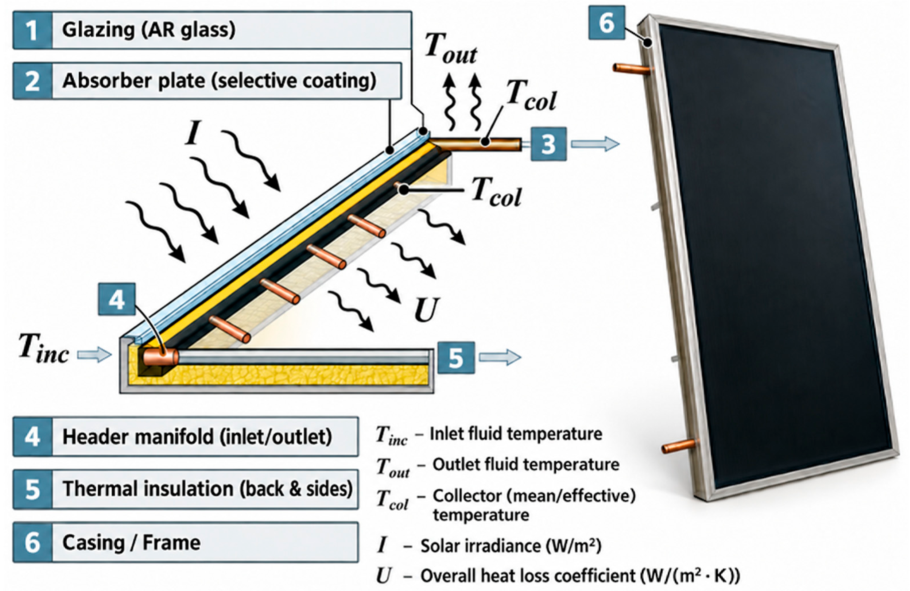
To illustrate the thermal and hydraulic connections used in the model, Figure 1 shows a typical diagram of a solar hot water system with forced circulation. This diagram illustrates the relationship between a flat-plate solar collector, a storage tank with a heat exchanger, a circulation pump, and connecting pipes, and serves as the physical basis for constructing the presented mathematical model.

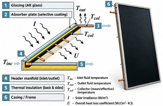
Figure 1. Schematic representation and photograph of the flat-plate solar collector. 1—glazing AR glass; 2—absorber plate with selective coating; 3—heat-loss direction; 4—header manifold (inlet/outlet); 5—thermal insulation (back and sides); 6—casing/frame. The black wavy arrows indicate incident solar radiation and heat losses, while the horizontal arrows show fluid flow directions. T_inc and T_out denote the inlet and outlet fluid temperatures, respectively; T_col represents the mean collector temperature; I is the solar irradiance (W/m²); and U is the overall heat-loss coefficient (W/(m²·K)).

Figure 1 shows a typical solar hot water system with forced circulation. A flat-plate solar collector absorbs solar radiation I and heats the heat carrier: it enters the collector at T_in,c and exits at T_out, with some heat lost to the environment through the total heat loss coefficient U. The heated heat carrier enters the storage tank equipped with a heat exchanger (coil), where it transfers heat to the water in the tank: the temperature of the water in the tank is denoted by T_st, and the temperature of the heat carrier in the return line (after the heat exchanger) is T₁. Circulation within the loop is provided by a pump that circulates the heat carrier through the collector and the coil, facilitating the transfer of energy from the collector to the tank; the photo on the right shows a laboratory setup featuring a collector, a tank/reservoir, and measuring instruments for monitoring temperatures and system operation.

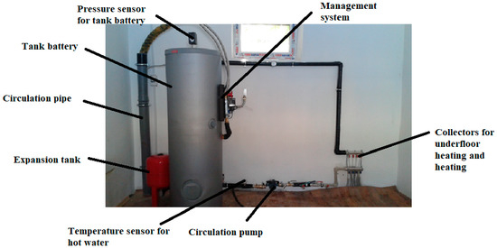
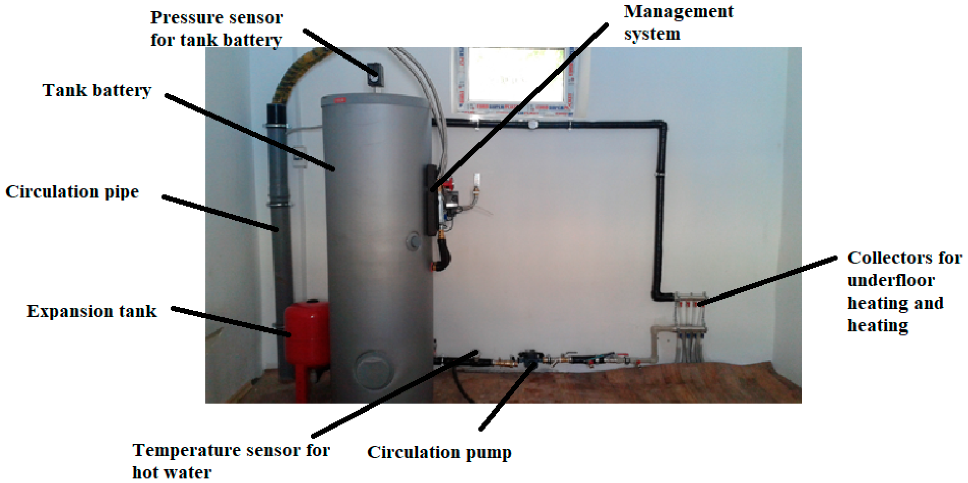
Figure 2 shows an experimental solar thermal system designed to heat water, store thermal energy, and transfer it to a heating system. The main component is a storage tank, in which the heated heat carrier is stored. A pressure sensor and a hot water temperature sensor are used to monitor the system’s operation. The circulation pump circulates the heat carrier through the pipes, while the expansion tank compensates for changes in the fluid’s volume caused by heating. Shown on the right is the collector assembly connected to the floor heating and room heating systems. Thus, the system shown here constitutes a fully fledged research test bed for analyzing the processes of solar thermal energy storage and utilization. It can be used for experimental evaluation of temperature regimes, studying the operation of the circulation pump, analyzing the effect of heat carrier pressure and flow rate on system efficiency, as well as for developing and testing automatic control algorithms.

Figure 2. Experimental solar thermal system.

The scientific novelty of this work lies in the development of a mathematical model of a solar water-heating system with pump circulation that accounts for the combined influence of variable solar radiation, ambient temperature, heat loss, and pump control mode on the formation of useful heat flux over a 24 h cycle. Unlike simplified approaches, the proposed model allows the system to be analyzed as a non-stationary thermal system with interrelated energy and operating parameters. Another novel aspect is the use of residual error to assess the model’s adequacy and confirm its applicability for predicting the operating characteristics of a solar water-heating system.

3. Validation Result

The developed model was validated to confirm its ability to accurately reproduce the actual thermal processes in a solar hot water supply system. To this end, daily profiles of input conditions, the system’s calculated thermal performance characteristics, and the errors between the simulated and measured output temperature values were analyzed. Particular attention was paid to the consistency of heat transfer dynamics, the nature of changes in heat loss, and the accuracy of the circulation pump control algorithm. The obtained validation results allow us to assess the reliability of the proposed model and its suitability for further calculations, optimization of operating modes, and the creation of a digital twin of the system.

To briefly present the validation results, the main characteristics are summarized in Table 1.

Table 1. Summary of daily profiles for the system’s input, output, and operating parameters.

№	Parameter	Designation	Interval	Range	Characteristic Values	Brief Interpretation
1	Solar radiation	Ir, W/m2	0–24 h	0–~880	max ~870–880 at 12–13 h; at night ≈0	Daytime bell-shaped profile: intensity increases after ~6 h, peaks around noon, and decreases by ~17 h.
2	Air temperature	Tair, °C	0–24 h	~3–~17	min ~3 at 3–4 h; max ~16.5–17 at ~15 h	A smooth daily variation with a near-sinusoidal dependence: a minimum in the early morning and a maximum in the afternoon.
3	Heat transfer coefficient	U, W/m2·K	0–24 h	~8.1–~11.0	max ~10.8–11.0 at 12–14 h; min ~8.1–8.3 at night	There are random fluctuations against the background of a general increase during the daytime and a decrease in the evening; the parameter changes within a relatively narrow range.
4	Heat flux of the heat exchanger	QHX, kW	0–24 h	0–~0.64	max ~0.63–0.64 about 12–13 h; outside working hours ≈ 0	Zero values at night and after the end of the day cycle; in the working interval of ~8–16 h, the heat flow increases and then decreases.
5	Residual Error	Residual (Sim—Meas) for Tout, °C	1 January 2026 … 8 January 2026	~−1.2–+1.1	average around 0; occasional deviations of up to ±1.1–1.2	The residuals are distributed around zero with no clear trend, indicating acceptable agreement between modelling and measurements.
6	Pump state	Pump state (0/1)	1 January 2026 … 8 January 2026	0 or 1	periodic switching between 0 and 1 approximately once a day	Binary pump operation mode: switching on and off is repeated cyclically, which corresponds to a regular daily control algorithm.

Table 1 presents the main quantitative characteristics obtained from the analysis of six graphs depicting the daily variation in input climatic influences, the system’s thermal parameters, the control signal, and the model’s residual error. The tabular format allows the graphical information to be summarized in a compact and easily comparable form, highlighting the minimum, maximum, and characteristic intervals of variation for the quantities under study. The data obtained show a consistent variation in solar radiation, ambient temperature, heat loss coefficient, and useful heat flux over the course of a day, and also confirm the pump’s stable cyclic operating mode. Furthermore, the analysis of the residual error indicates a satisfactory agreement between the simulation results and the measured values and can be used for subsequent validation of the developed model.

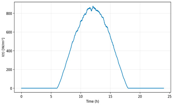
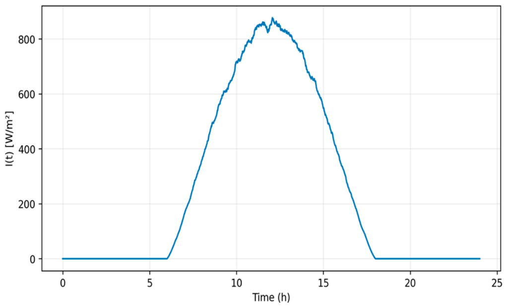
Figure 3 shows the daily variation in solar irradiance, depending on the time of day. During the night and early morning hours, the radiation intensity is almost zero, and then it begins to increase rapidly around 7 h. The maximum value is reached near noon, at around 850–870 W/m², which corresponds to the period of maximum solar activity. After 13–14 h, there is a gradual decrease in irradiance, and by evening, after about 18 h, the value approaches zero again. This profile is typical for a clear day and can be used as an input function for modelling solar thermal systems.

Figure 3. Daily variation in solar irradiance depending on the time of day.

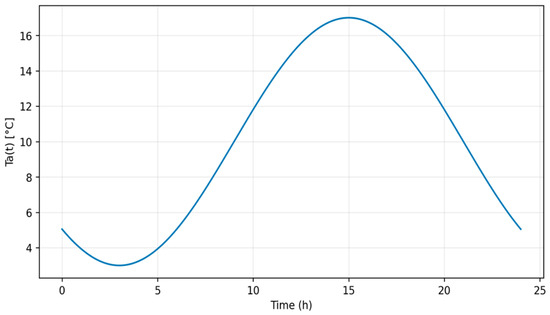
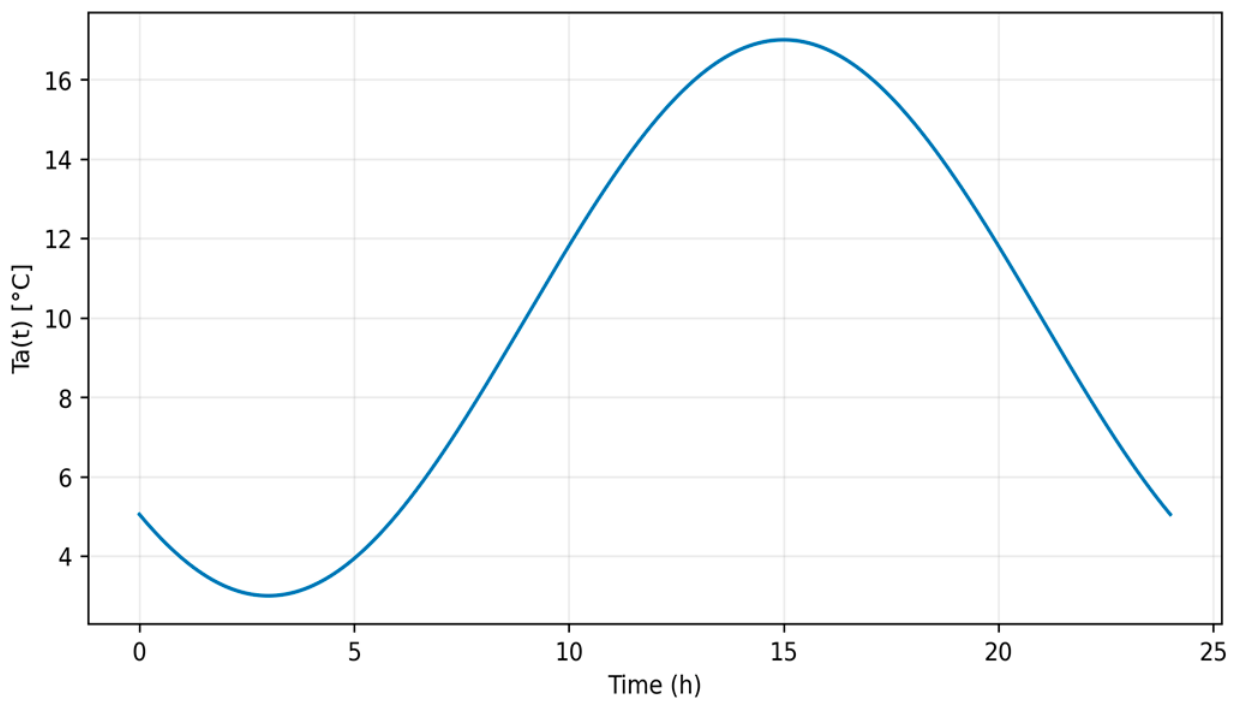
Figure 4 shows the daily change in ambient temperature as a function of time. The minimum value is observed during the night and early morning hours, at around 3 °C, after which the temperature gradually increases. The maximum is reached in the afternoon, around 15–16 h, at around 16.5–17 °C. The temperature then gradually decreases in the evening and at night, which corresponds to a typical daily temperature cycle and can be used as an input parameter in thermal modelling of a solar collector.

Figure 4. Daily change in ambient temperature depending on time.

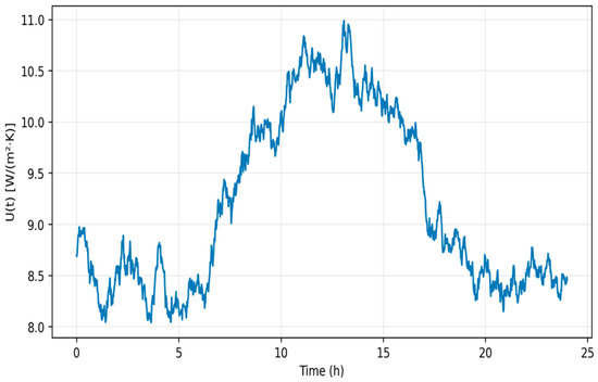
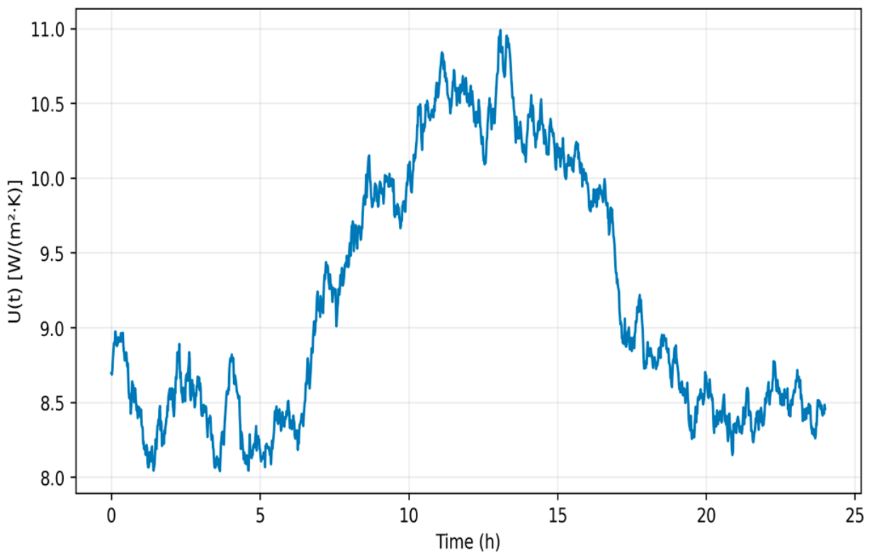
Figure 5 shows the daily variation in the total heat loss coefficient. During the night and early morning hours, its value remains at a relatively low level, around 8.1–8.8 W/(m²·K), after which a noticeable increase is observed in the first half of the day. The maximum is reached approximately in the range of 12–14 h and amounts to about 10.8–11.0 W/(m²·K). In the afternoon, the coefficient gradually decreases and, by evening, returns to values in the range of 8.4–8.7 W/(m²·K). This pattern of change reflects the daily dynamics of the collector’s heat loss and can be used to more accurately model its thermal efficiency.

Figure 5. Daily change in the total heat loss coefficient.

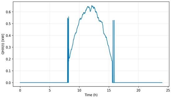
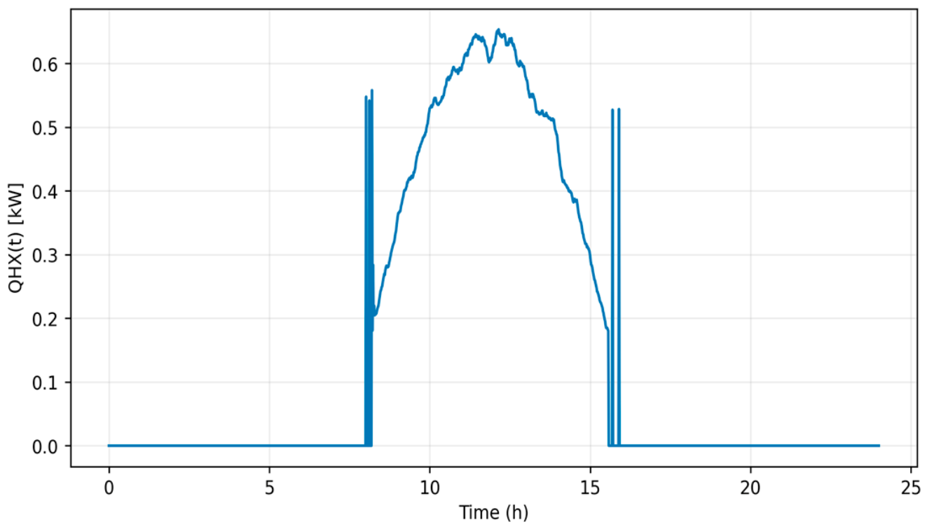
Figure 6 shows the daily variation in heat loss. During nighttime hours and periods of no solar activity, heat loss is practically zero, whereas a sharp increase is observed starting around 8 h. The maximum is reached during the day, around 12–13 h, and amounts to approximately 0.63–0.65 kW, after which the heat loss gradually decreases. By evening, around 16 h, the value tends to drop back to zero, reflecting a decrease in the system’s heat output and a reduction in the temperature difference with the surrounding environment.

Figure 6. Daily change in heat loss capacity.

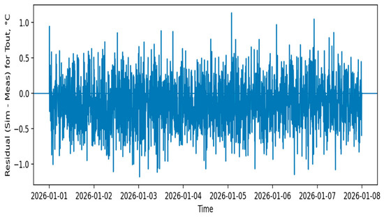
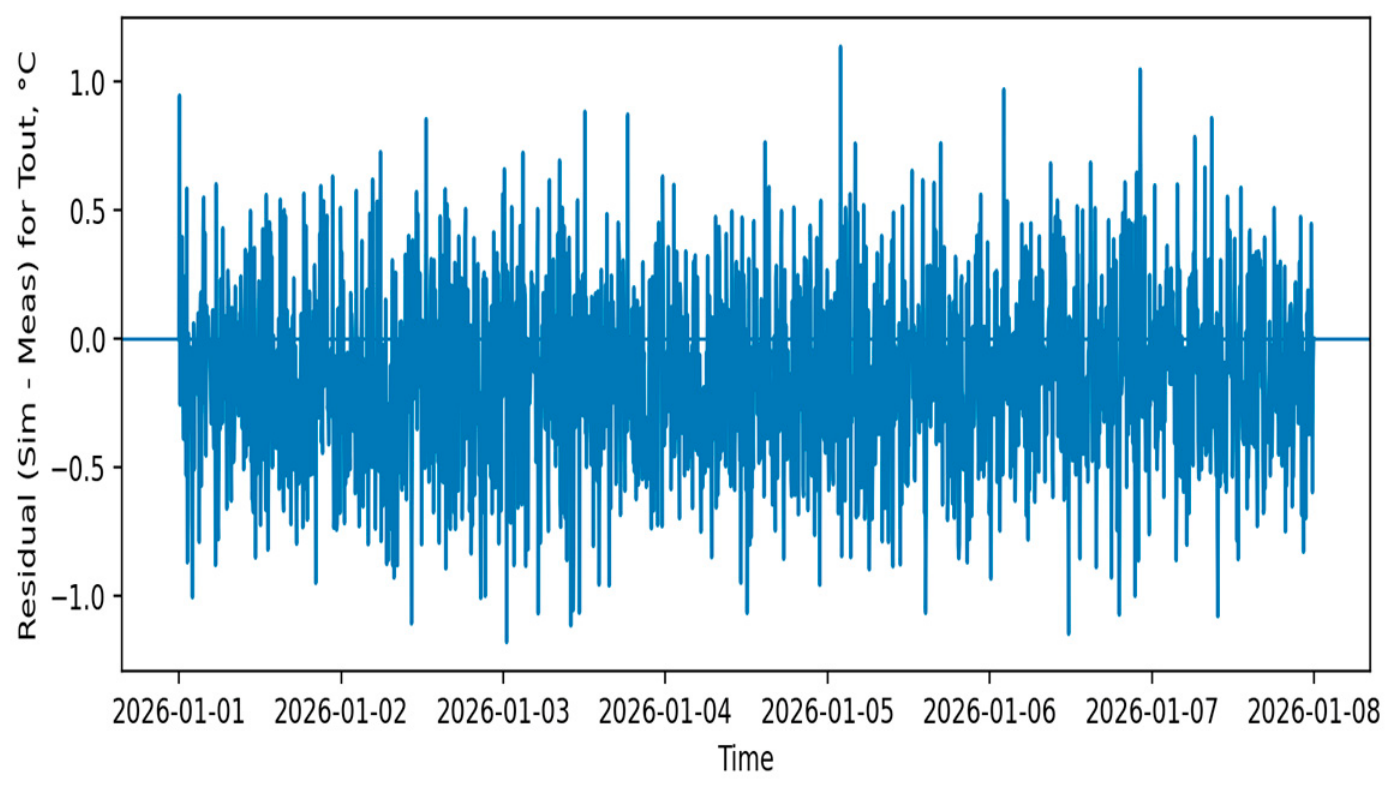
Figure 7 shows the model residuals for the output temperature. It can be seen that the values of e(t) fluctuate near zero without a distinct trend, indicating the absence of a noticeable systematic bias between the calculated and experimental data. Most deviations fall within a relatively narrow range, which means that the model generally adequately describes the dynamics of the output temperature, and the main errors are random in nature.

Figure 7. Model residuals for the output temperature.

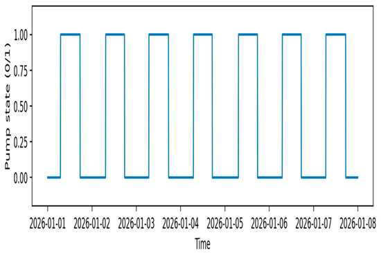
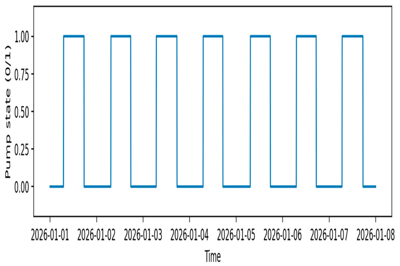
Figure 8 shows the change in the pump’s state over time, where a value of 0 corresponds to the off state and a value of 1 corresponds to the on state. It can be seen that the pump operates in a cyclic mode, periodically switching between the on and off states throughout the entire interval under consideration. This switching pattern indicates discrete control of the system, in which the pump is activated only at specific intervals, for example, when a temperature or energy condition is met.

Figure 8. Change in the pump’s state over time.

Overall, the results confirm the effectiveness of the developed mathematical model and its suitability for analyzing the daily dynamics of a solar water-heating system with pump circulation. The identified relationships between solar radiation intensity, temperature conditions, heat loss, and useful heat flux make it possible to use the model to predict the system’s operational performance, select optimal pump control modes, and improve the plant’s energy efficiency.

4. Discussion

The developed model was validated by comparing the calculated and measured outlet temperatures of the solar water-heating system. As previously noted in this article, the model validation involved analyzing daily profiles of input conditions, the system’s calculated thermal characteristics, and the errors between the simulated and measured temperature values. This approach allows for the assessment not only of the accuracy of temperature calculations but also of the correctness of the reproduction of the main thermal processes in the system. Analysis of the residual error showed that most deviations between calculated and measured values fall within approximately ±1.0 °C, while individual deviations reach about ±1.1–1.2 °C. At the same time, the residuals are distributed around zero and do not exhibit a pronounced systematic trend, which indicates the absence of a noticeable model offset and confirms the acceptable agreement between the simulation results and the experimental data. Additionally, the model’s accuracy is confirmed by the fact that the calculated daily profiles of solar radiation, air temperature, heat loss coefficient, and net heat flux are physically consistent. Maximum values of solar radiation and heat flux are observed during the daytime, while at night and in the evening hours, the system’s thermal activity decreases. This pattern of parameter changes corresponds to the typical operation of solar water-heating systems and confirms the validity of the proposed model. Particular attention is paid to verifying the control algorithm for the circulation pump. According to the simulation results, the pump operates in a discrete cyclic mode with 0/1 states, which corresponds to the logic of switching on and off when specified temperature or energy conditions are met. This demonstrates that the model can be used not only to calculate thermal parameters but also to analyze heat carrier circulation control modes. Thus, the validation results confirm the satisfactory adequacy of the developed model. The model can be used to predict the thermal efficiency of a solar water-heating system, select an optimal pump operating mode, analyze the influence of climatic factors, and further develop a digital twin or an intelligent control system.

5. Conclusions

The mathematical model of a solar water-heating system with pump circulation that was developed made it possible to identify the patterns of change in its key operating parameters under non-stationary daily conditions. Unlike simplified descriptive approaches, the proposed model provides a comprehensive analysis of the interrelationships between external climatic influences, heat losses, useful heat flux, and the circulation mode of the heat carrier, thereby enhancing the reliability of the system performance analysis. The study found that the system’s energy efficiency is determined not by a single parameter, but by the combined effect of solar radiation intensity, ambient temperature, and the pump activation algorithm. It has been shown that it is precisely the coordination of the circulation mode with the current thermal state of the system that allows for a more efficient use of incoming solar energy and reduces heat losses during transient conditions. This confirms that pump control should be considered a key factor in improving the overall efficiency of a solar water-heating system. A comparison of theoretical and experimental data revealed satisfactory agreement between the results, confirming the validity of the developed model and its suitability for solving practical engineering problems. The proposed approach can be applied to preliminary design, the selection of optimal operating modes, the analysis of the influence of climatic factors, and the further optimization of solar water-heating system parameters. The practical significance of this work lies in the fact that the results obtained can serve as a basis for improving solar heating systems under conditions of variable insolation and changing ambient temperatures.

References

- Yoo, J.H. Evaluation of solar hot water heating system applications to high-rise multi-family housing complex based on three years of system operation. Energy Build. 2015, 101, 54–63. [Google Scholar] [CrossRef] [Scilit]
- Chow, T.; Fong, K.; Chan, A.; Lin, Z. Potential application of a centralized solar water-heating system for a high-rise residential building in Hong Kong. Appl. Energy 2006, 83, 42–54. [Google Scholar] [CrossRef] [Scilit]
- Badescu, V. Simulation analysis for the active solar heating system of a passive house. Appl. Therm. Eng. 2005, 25, 2754–2763. [Google Scholar] [CrossRef] [Scilit]
- Siddiqui, M.; Said, S. A review of solar powered absorption systems. Renew. Sustain. Energy Rev. 2015, 42, 93–115. [Google Scholar] [CrossRef] [Scilit]
- Kalogirou, S. Solar thermal collectors and applications. Prog. Energy Combust. Sci. 2004, 30, 231–295. [Google Scholar] [CrossRef] [Scilit]
- Maldonado, R.; Huerta, E.; Corona, J.; Ceh, O.; Leon, A.; Henandez, I. Design and construction of a solar flat collector for social housing in México. Energy Procedia 2014, 57, 2159–2166. [Google Scholar] [CrossRef] [Scilit][Green Version]
- Nogueira, C.; Vidotto, M.; Toniazzo, F.; Debastiani, G. Software for designing solar water heating systems. Renew. Sustain. Energy Rev. 2016, 58, 361–375. [Google Scholar] [CrossRef] [Scilit]
- Farahat, S.; Sarhaddi, F.; Ajam, H. Exergetic optimization of flat plate solar collectors. Renew. Energy 2009, 34, 169–1174. [Google Scholar] [CrossRef] [Scilit]
- Luminosu, I.; Fara, L. Determination of the optimal operation mode of a flat solar collector by exergetic analysis and numerical simulation. Energy 2005, 30, 731–747. [Google Scholar] [CrossRef] [Scilit]
- Park, S.; Pandey, A.; Tyagi, V.; Tyagi, S. Energy and exergy analysis of typical renewable energy systems. Renew. Sustain. Energy Rev. 2014, 30, 105–123. [Google Scholar] [CrossRef] [Scilit]
- Yedilkhan, A.; Murat, K.; Beibut, A.; Aliya, K.; Ainur, K.; Tumur, M.; Azhibek, D. Mathematical justification of thermosyphon effect main parameters for solar heating system. Cogent Eng. 2020, 7, 1851629. [Google Scholar] [CrossRef] [Scilit]
Disclaimer/Publisher’s Note: The statements, opinions and data contained in all publications are solely those of the individual author(s) and contributor(s) and not of MDPI and/or the editor(s). MDPI and/or the editor(s) disclaim responsibility for any injury to people or property resulting from any ideas, methods, instructions or products referred to in the content. |
© 2026 by the authors. Licensee MDPI, Basel, Switzerland. This article is an open access article distributed under the terms and conditions of the Creative Commons Attribution (CC BY) license.