


Abstract
Sweep frequency response analysis (SFRA) is interpreted by comparison, so the choice of reference strongly affects what can be inferred from a change in the response. This paper develops a quantitative workflow aligned with the reference hierarchy of CIGRE Technical Brochure 812. The method combines log-frequency weighting, five one-decade bands, separation of vertical offset from shape change, and robustness checks. A 54-trace dataset was used to quantify same-asset and cross-unit variability, and a separate 66-trace longitudinal case spanned a documented differential protection event. The median equal-decade RMSE was 0.793 dB for repeated measurements of the same transformer and 5.326 to 7.364 dB for cross-unit comparisons. In the longitudinal case, six of 11 comparison families showed a robust change onset below 20 kHz. Median shape RMSE increased from 1.203 dB in D3 to 3.303 dB in D4 and 5.900 dB in D5, while weighted correlation fell to 0.944 and 0.793 in D4 and D5. These results show that reference quality, frequency localization, and robustness should be considered together when SFRA differences are quantified. The reported values are case-specific and are not proposed as universal diagnostic thresholds.
1. Introduction
Sweep frequency response analysis (SFRA) is a comparative diagnostic technique for detecting changes in transformer winding and magnetic structures. IEEE C57.149-2024 and IEC 60076-18:2012 define instrumentation, connections, procedures, analysis, and data management requirements [1,2], but an SFRA signature does not independently establish condition and must be interpreted against an appropriate reference.
CIGRE TB 812 provides the interpretive framework used here, prioritizing a previous measurement of the same transformer, an identical or similar unit, and homologous phases, while requiring test setup, transformer state, tap position, temperature, and external conditions to be considered before differences are attributed to deterioration [3]. CIGRE TB 342 provides earlier measurement practices and mechanical condition examples [4].
TB 812 also notes that numerical index behavior depends on sensitivity, monotonicity, frequency range, and data size, so universal thresholds are not justified [3]. Prior work has reviewed FRA interpretation and numerical indices [5,6], cross-test comparison [7], and statistical assessment [8]. Recent studies have used small frequency windows for fault discrimination [9], resonance/antiresonance-based indices and frequency range selection [10], surveyed numerical indices, modeling, transfer function estimation, and AI-based interpretation [11], and applied Six Sigma statistics across defined frequency regions [12].
Against this background, we ask how quantitative comparison changes when the available reference shifts from a previous measurement of the same asset to sister-unit and broader design-family references, then apply the same framework to a longitudinal field case associated with a documented protection event. The contribution is a reference-aware workflow combining log-frequency weighting, five equal decades, vertical-offset/shape decomposition, and robustness checks to quantify reference-dependent variability and persistent frequency-localized change without assigning a unique defect or universal threshold.
2. Materials and Methods
2.1. Field SFRA Dataset and Case Definition
Five field .frax files were used to study reference selection. F11 and F03 are repeat measurements of the same mobile transformer; F04 and F05 form the closest sister-unit pair; and F02 provides a broader design-family comparison. Together, these campaigns contain 54 traces. Nine test configurations are common to all five files and were used for the reference selection comparisons; additional interwinding responses from F02, F04, and F05 were retained for supporting analysis.
Two 33-trace campaigns from the same DACHI autotransformer were measured on 17 April 2025 and 23 July 2026; a differential protection trip occurred on 16 August 2025, and the post-event report classified DGA as Status 3 with unacceptable dielectric power-factor/capacitance results. Different FRAX instruments (Megger Sweden AB, Danderyd, Sweden) were used. Reference-campaign metadata identify S/N 2201636; and a FRAX 101 certificate documents source-frequency calibration 141 days before that test, although its serial field is blank. Follow-up S/N 1500876 is explicitly identified in calibrations 316 days before and 40 days after its test; the pre-test report spans 10 Hz–2 MHz. No direct inter-instrument cross-check was documented, so interpretation emphasized persistent frequency-localized changes across related configurations. The main characteristics and analytical roles of the field SFRA cases are summarized in Table 1.
Table 1.
Main characteristics and analytical role of the field SFRA cases.
2.2. FRAX File Extraction and Data Validation
Custom Python scripts parsed .frax XML files to extract frequency, channel amplitudes, amplitude ratio, phase difference, and channel phases. Magnitude (dB) and transfer phase were reconstructed and cross-checked from channel data. Across both datasets, 120 traces contained 1051 samples over approximately 20 Hz–2 MHz; native paired grids were retained without interpolation. Analysis was conducted and figures were designed using Python 3.13.0 (Python Software Foundation, Beaverton, OR, USA). ChatGPT (GPT-5.0, OpenAI, San Francisco, CA, USA; accessed in 2026) assisted Python coding and language editing; the author reviewed and validated code, outputs, and manuscript text. No artificial intelligence or machine learning model formed part of the SFRA analytical or diagnostic methodology; all processing, indices, onset estimation, and robustness analyses followed the numerical and statistical procedures described below.
2.3. Frequency Bands and Log-Frequency Weighting
The range was divided into five decades: D1, 20–200 Hz; D2, 200 Hz–2 kHz; D3, 2–20 kHz; D4, 20–200 kHz; and D5, 200 kHz–2 MHz. Their unequal densities (50, 101, 199, 300, and 401 points) would bias an unweighted full-range metric toward high frequencies.
Trapezoidal weights were therefore calculated on the log10-frequency axis and normalized within each interval, followed by equal weighting of the five decades. Because TB 812 notes that universal frequency regions are difficult to define [3], these decades were used only as transparent numerical intervals; leave-one-band-out analysis tested sensitivity to their selection.
2.4. Pairwise Difference Metrics
For homologous responses A and B, the pointwise magnitude difference and log-frequency-weighted RMSE were defined by Equation (1). The remaining weighted metrics included MAE, signed offset, maximum absolute difference, magnitude correlation, and wrapped phase difference.
The five band-specific RMSE values were combined with equal decade weighting according to Equation (2).
2.5. Separation of Vertical Offset and Shape Deformation
The magnitude difference was decomposed into a weighted mean vertical offset (Equation (3)) and residual shape RMSE (Equation (4)). We further define , the fraction of weighted squared magnitude difference remaining after offset removal; it is not physical energy, a fault-severity metric, or a defect assignment.
2.6. Longitudinal Field-Event Assessment
For the longitudinal case, 33 reference/follow-up traces were paired by terminals and configuration. Bandwise offset-corrected shape RMSE and magnitude correlation used the same log-frequency weighting, while sliding log-frequency windows supplemented the fixed decades. Onset sensitivity covered all 18 combinations of 0.20/0.30/0.40-decade windows, 0.50/0.75/1.00 dB minimum-change floors, and persistence of 3/4 consecutive windows. These were sensitivity settings, not physical diagnostic thresholds. Resonance/antiresonance landmarks provided a second spectral descriptor. The measures localized and characterized change without assigning an automatic fault class.
2.7. Robustness and Sensitivity Analyses
To test whether the reference hierarchy depended on a small part of the dataset, each of the nine configurations and each frequency band was omitted in turn. We also performed 10,000 paired bootstrap resamples using the same configuration indices. The resulting 2.5th to 97.5th percentile intervals describe stability to configuration selection; they are not population-level confidence intervals because the test configurations are not independent samples.
3. Results
3.1. Dataset Integrity and Common Analysis Set
All files passed the parsing and consistency checks. The reference-selection dataset contains 54 traces; 45 of them form the nine-configuration set common to all five campaigns. The longitudinal dataset adds 66 traces, paired into 33 reference/follow-up comparisons. Every trace contains 1051 samples over approximately 20 Hz to 2 MHz, and the paired comparisons have identical frequency grids.
3.2. Same-Asset Field Variability
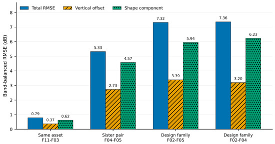
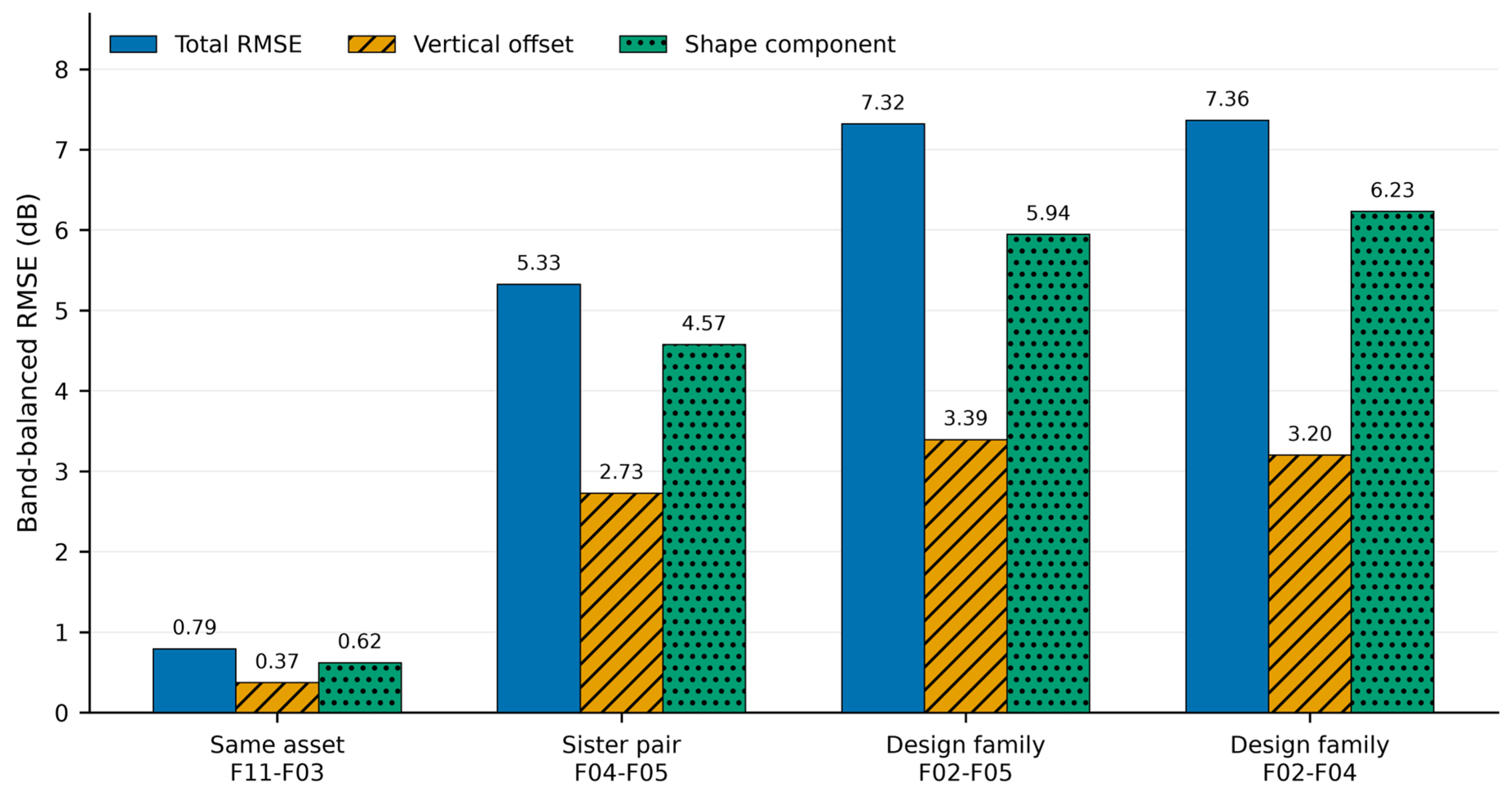
Repeated measurements of the same transformer (F11–F03) gave a median equal-decade RMSE of 0.793 dB with a descriptive bootstrap interval of 0.659 to 0.942 dB. The median offset and shape components were 0.371 and 0.620 dB. Leave-one-trace values ranged from 0.766 to 0.826 dB, and leave-one-band values from 0.663 to 0.887 dB. F11–F03 remained the least-different comparison in every sensitivity run.
3.3. Cross-Unit Comparisons
The closest sister-unit pair, F04–F05, gave a median equal-decade RMSE of 5.326 dB (4.756 to 6.341 dB), 6.71 times the same-asset result. The broader design-family comparisons F02–F05 and F02–F04 gave 7.318 and 7.364 dB, respectively, corresponding to 9.22 and 9.28 times the same-asset result.
F04–F05 was also lower than F02–F05 and F02–F04 in 99.87% and 99.85% of the paired bootstrap resamples, respectively. It remained the closest cross-unit comparison in every leave-one-trace and leave-one-band analysis. Only the order of F02–F05 and F02–F04 changed, and only when a trace or D4 was omitted. The band-balanced comparison metrics are summarized in Table 2, and Figure 1 illustrates the median total RMSE together with the vertical-offset and shape components.
Table 2.
Band-balanced comparison metrics. Stability intervals are descriptive 2.5th–97.5th percentile intervals from paired configuration resampling; robust ranks summarize leave-one-trace-out sensitivity.
Figure 1.
Median equal-decade total RMSE and median vertical-offset and shape components across the nine common SFRA configurations.
3.4. Vertical Offset and Shape Deformation
Offset removal showed that cross-unit differences were not merely level shifts. Low-frequency bands contained a larger offset component, whereas higher-frequency bands were dominated by shape change. For F04–F05, the median D4 shape fraction was 93.8%, meaning that 93.8% of the weighted squared magnitude difference remained after offset removal; this does not identify a specific defect.
3.5. Longitudinal Field-Event Case
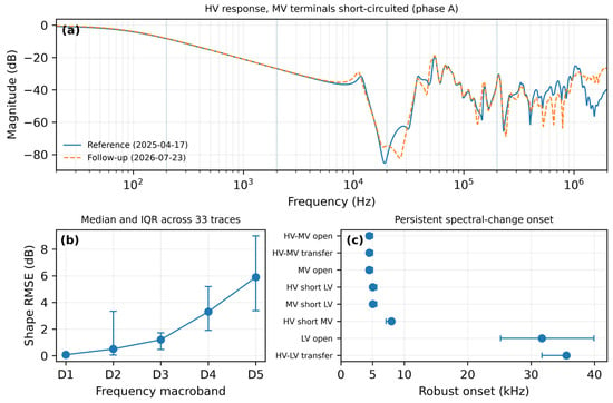
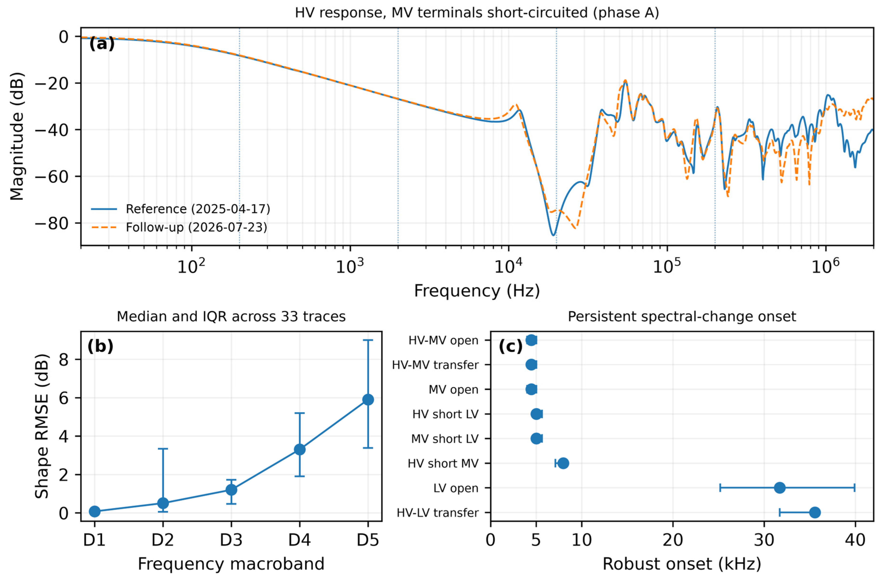
The longitudinal case showed frequency-progressive rather than isolated high-frequency change. Robust onset was obtained in 8 of 11 comparison families; 6 of 11 (54.5%) had robust median onset below 20 kHz, with the earliest at 4.48 kHz. Median shape RMSE increased from 1.203 dB in D3 to 3.303 dB in D4 and 5.900 dB in D5, while median correlation fell to 0.944 and 0.793 in D4–D5. Overall, 91.1% of reference landmarks were matched and the 90th-percentile absolute landmark shift was 5.28%. Figure 2 summarizes a representative response and these bandwise/onset results.
Figure 2.
Longitudinal assessment of the field-event case. (a) Reference and follow-up response for the short-circuit trace selected objectively as the largest D4 shape-RMSE change among the short-circuit measurements (H1-H0X0; X1-X2-X3 shorted); (b) median shape RMSE and interquartile range across 33 paired traces; (c) robust onset estimates for eight comparison families. Three additional families did not yield a stable onset. D1–D5 cover 20–200 Hz, 0.2–2 kHz, 2–20 kHz, 20–200 kHz, and 0.2–2 MHz.
3.6. Overall Robustness of the Comparison Hierarchy
F11–F03 remained the least-different comparison in every sensitivity run, and F04–F05 remained the closest cross-unit pair. Only the order of the two broader F02 comparisons changed in a limited number of leave-one-out cases. The stability intervals for the same-asset and closest cross-unit comparisons did not overlap: the lower bound for F04–F05 (4.756 dB) remained 3.814 dB above the upper bound for F11–F03 (0.942 dB), a conservative ratio of 5.05. This result describes stability to configuration selection; it is not a population-level significance test.
4. Discussion
4.1. Influence of Reference Selection
The same-asset RMSE of 0.793 dB is well below the 5.326 to 7.364 dB obtained between units, giving a quantitative example of why TB 812 places a previous measurement of the same transformer first in the reference hierarchy [3]. Unit-to-unit comparisons also contain manufacturing, tap, campaign, environmental, and unrecorded condition differences. For F04–F05, the reported tap metadata were non-equivalent (F04: position 1, LTC; F05: position 9, NLTC), so the 5.326 dB RMSE cannot isolate a tap-position contribution. F04–F05 nevertheless remained the closest cross-unit comparison in every sensitivity run; this supports ranking stability, not absence of tap influence. The non-overlapping descriptive intervals reinforce this within-dataset separation but do not define a universal decision threshold.
4.2. Frequency-Dependent Nature of Cross-Unit Differences
The offset-shape decomposition also shows why one full-range metric is incomplete: low-frequency differences can be dominated by level offsets, whereas higher-frequency differences can reflect resonance-shape changes. Consistent with TB 812 [3], equal-decade log-frequency weighting localizes this behavior without assigning a unique component or defect to any band.
4.3. Interpretation of the Longitudinal Field Event
Longitudinal changes emerged in several test families from roughly 4–8 kHz and increased through D4–D5, rather than being confined to the highest decade. This pattern is consistent with the documented differential protection trip, DGA Status 3, and unacceptable dielectric power-factor/capacitance results. However, SFRA cannot identify a unique fault or establish causality, particularly because intervention history was incomplete and a different FRAX instrument was used. The case is therefore interpreted as longitudinal evidence consistent with an abnormal history, not causal fault localization.
4.4. Practical Implications and Limitations
Several limitations remain. F04–F05 had non-equivalent tap metadata, so its RMSE cannot isolate a tap contribution. Historical campaigns did not uniformly control environment or intervention history. The longitudinal comparison used different FRAX instruments: reference S/N 2201636 has bounded pre-test source-frequency calibration evidence, whereas follow-up S/N 1500876 is bracketed by pre/post calibrations of the exact serial. No direct FRAX-to-FRAX cross-check or complete transfer-function magnitude/phase calibration was documented. The onset grid was exploratory, and bootstrap/leave-one-out analyses measure within-case robustness rather than population uncertainty. Independent validation is limited to one same-asset repeat pair, three related cross-unit transformers, and one longitudinal event; therefore, reported separation and onset behavior are case-specific and no universal threshold is proposed.
5. Conclusions
Two points emerge from this study. First, reference choice has a large quantitative effect: the same-transformer comparison was 0.793 dB, whereas cross-unit comparisons ranged from 5.326 to 7.364 dB and remained higher in every sensitivity analysis.
The longitudinal case shows that the same bandwise framework can localize persistent change: 6 of 11 families had robust onset below 20 kHz, while shape RMSE increased and correlation decreased with frequency. Log-frequency weighting, equal-decade aggregation, offset-shape decomposition, and robustness checks provide a traceable reference-aware comparison consistent with CIGRE TB 812 [3]. These field cases support the workflow, not universal thresholds; broader independent validation across repeat campaigns, matched sister units, transformer designs, operating states, and documented events is required before general transferability claims.
Funding
This research received no external funding.
Institutional Review Board Statement
Not applicable.
Informed Consent Statement
Not applicable.
Data Availability Statement
The processed datasets, analysis code, and numerical results supporting this study are available from the author upon reasonable request. The original field SFRA files and diagnostic report are subject to asset-owner confidentiality requirements and can be shared only when the necessary authorization is available.
Conflicts of Interest
The author is employed by Megger as an Applications Engineer and Repair Technical Support specialist for Latin America. The field measurements analyzed in this study were acquired with Megger FRAX instruments. The study was conducted independently and received no dedicated financial or material support from Megger. Megger had no role in case selection, study design, data processing, analysis, interpretation, manuscript preparation, or the decision to submit the work.
References
- IEEE Std C57.149-2024; IEEE Guide for the Application and Interpretation of Frequency Response Analysis for Oil-Immersed Transformers. IEEE: New York, NY, USA, 2025.
- IEC 60076-18:2012; Power Transformers—Part 18: Measurement of Frequency Response. IEC: Geneva, Switzerland, 2012.
- CIGRE Working Group A2.53; Advances in the Interpretation of Transformer Frequency Response Analysis (FRA). Technical Brochure 812; CIGRE: Paris, France, 2020.
- CIGRE Working Group A2.26; Mechanical-Condition Assessment of Transformer Windings Using Frequency Response Analysis (FRA). Technical Brochure 342; CIGRE: Paris, France, 2008.
- Picher, P.; Tenbohlen, S.; Lachman, M.; Scardazzi, A.; Patel, P. Current State of Transformer FRA Interpretation: On Behalf of CIGRE WG A2.53. Procedia Eng. 2017, 202, 3–12. [Google Scholar] [CrossRef] [Scilit]
- Samimi, M.H.; Tenbohlen, S. FRA Interpretation Using Numerical Indices: State-of-the-Art. Int. J. Electr. Power Energy Syst. 2017, 89, 115–125. [Google Scholar] [CrossRef] [Scilit]
- Banaszak, S.; Szoka, W. Cross Test Comparison in Transformer Windings Frequency Response Analysis. Energies 2018, 11, 1349. [Google Scholar] [CrossRef] [Scilit]
- Tahir, M.; Tenbohlen, S.; Miyazaki, S. Analysis of Statistical Methods for Assessment of Power Transformer Frequency Response Measurements. IEEE Trans. Power Deliv. 2021, 36, 618–626. [Google Scholar] [CrossRef] [Scilit]
- Vosoughi, A.; Samimi, M.H. Transformer fault type discrimination based on window calculation method and frequency response analysis. Measurement 2022, 202, 111889. [Google Scholar] [CrossRef] [Scilit]
- Samimi, M.H.; Faiz, J.; Ghasemi Parchini, J. Feasibility Study on the Detection of Turn-to-Turn Fault Severity in the Transformer Winding by Frequency Response Analysis and Numerical Indices. Electr. Power Compon. Syst. 2023, 51, 856–870. [Google Scholar] [CrossRef] [Scilit]
- Faiz, J.; Naseri, H.; Tayyari Ilaghi, H.; Samimi, M.H. Frequency Response Analysis-Based Transformer Condition Monitoring Supported by Artificial Intelligence—A Review. IET Sci. Meas. Technol. 2025, 19, e70014. [Google Scholar] [CrossRef] [Scilit]
- Thango, B.A. Six Sigma-Based Frequency Response Analysis for Power Transformer Winding Deformation. Appl. Sci. 2025, 15, 3951. [Google Scholar] [CrossRef] [Scilit]

Disclaimer/Publisher’s Note: The statements, opinions and data contained in all publications are solely those of the individual author(s) and contributor(s) and not of MDPI and/or the editor(s). MDPI and/or the editor(s) disclaim responsibility for any injury to people or property resulting from any ideas, methods, instructions or products referred to in the content. |
© 2026 by the author. Licensee MDPI, Basel, Switzerland. This article is an open access article distributed under the terms and conditions of the Creative Commons Attribution (CC BY) license.