Design-Oriented Model for Estimating Current Density in Oil-Cooled End Windings ^†

Abstract

Efficient thermal management of electric traction machines is increasingly important as higher power density and reliability requirements push winding temperatures close to their limits, particularly in the end-winding region. However, fast design-oriented procedures linking parametric hairpin winding geometry to simplified winding-temperature estimation and finite element verification remain limited. This paper presents an automated workflow for generating a parametric hairpin end-winding model, combined with an analytical method for estimating the current density for a known heat-transfer coefficient on the end-winding surface. A finite-element thermal model of the same geometry is then developed for comparison. Parametric analyses are performed using both approaches, including an assessment of the sensitivity to the assumed heat-transfer coefficient and the results are presented as parametric sensitivity plots suitable for preliminary design assessment. The proposed method enables rapid preliminary assessment of parametric trends and direct comparison between analytical and finite-element thermal predictions.

1. Introduction

The increasing power density of electric traction machines places growing demands on thermal management. Compact active parts and higher electromagnetic loading increase heat generation in a limited volume, while insulation temperature limits restrict the maximum continuous operating point. Thermal constraints therefore remain one of the key limits in modern traction-drive designs [1,2].

The end-winding region is particularly critical because its heat-removal paths are less effective than those in the active slot region [3,4]. This issue is important for hairpin windings, which are widely used in high-performance traction machines due to their high slot fill factor and manufacturability [5,6,7]. Their compact geometry and high current density can, however, produce local hot spots [8,9].

Direct oil cooling is a promising solution for improving heat removal from end windings. Spray, jet, and drip configurations can deliver coolant directly to thermally loaded surfaces and increase the local heat-transfer coefficient [10,11,12]. In practical hairpin arrangements, however, only part of the end-winding surface is effectively exposed to oil, so the cooled surface area must be considered in the thermal model [8,12].

Detailed finite element analysis (FEA) models provide useful local temperature information, but they are often too time-consuming for repeated design iterations. Analytical or reduced-order models are faster, but they may neglect geometric effects and non-uniform cooling [4,13,14]. A design-oriented workflow linking parametric hairpin geometry, rapid current density estimation, and finite-element verification is therefore needed.

This paper proposes such a framework for oil-cooled hairpin end windings. Its main contributions are an automatically generated parametric end-winding geometry, an analytical model for estimating the current density for a known surface heat-transfer coefficient, a finite-element thermal model derived from the same geometry, and a parametric comparison of both approaches using sensitivity analyses.

2. Parametric Geometry and Analytical Model of a Hairpin Winding

This section describes the parametric geometry of the hairpin end winding and its use in the analytical thermal model. The geometry is generated automatically from a set of design parameters. Based on this geometry, the conductor volume, heat-generating region, and effective cooled surface area are evaluated. These quantities are then used in the analytical model to estimate the current density for a prescribed heat-transfer coefficient.

2.1. Parametric Hairpin Winding Geometry

Before generating the parametric hairpin end-winding geometry, the main input variables must first be defined. These variables, summarized in Table 1, describe the conductor dimensions, stator geometry, and end-winding region. The parametric model represents one half of the machine in the axial direction due to the assumed geometric symmetry. The procedure for calculating the parametric model is based on [15].

Table 1. List of input variables for the parametric model of a hairpin winding.

Variable	Description
hs	Height of one rectangular conductor of the hairpin winding
ds	Width of one rectangular conductor of the hairpin winding
Q1	Total number of stator slots
Qc	Coil pitch expressed as the number of stator slots between two coil sides
Lfe	Axial length of the stator core
Lfe,out	Length of the straight conductor part protruding from the stator core
Rc	Mean radius of the end-winding circular path
Lkc	Perpendicular distance from the stator core to the end of the end winding

The angular span corresponding to the coil pitch is determined from the total number of stator slots and the coil pitch as

$$\alpha ={\displaystyle \frac{360°}{Q_1}}{Q}_{\mathrm{c}}.$$

(1)

The circular end winding length is determined based on the mean radius of the end winding and the coil pitch angle using the formula

$$S_{\mathrm{l}\mathrm{c}}=2R_{\mathrm{c}}\sin \left({\displaystyle \frac{\alpha }{2}}\right).$$

(2)

The length of one inclined part of the end winding is calculated using the chord length and the axial end-winding extension as

$$L_{\mathrm{i}\mathrm{n}\mathrm{c}}=\sqrt{{\left({\displaystyle \frac{S_{\mathrm{l}\mathrm{c}}}{2}}\right)}^2+{\left(L_{\mathrm{k}\mathrm{c}}-L_{\mathrm{f}\mathrm{e},\mathrm{o}\mathrm{u}\mathrm{t}}\right)}^2}.$$

(3)

The total conductor length is obtained by summing the active axial length, the straight protruding parts, and both inclined end-winding sections as

$$L_{\mathrm{t}\mathrm{o}\mathrm{t}}=L_{\mathrm{f}\mathrm{e}}+2L_{\mathrm{f}\mathrm{e},\mathrm{o}\mathrm{u}\mathrm{t}}+2L_{\mathrm{i}\mathrm{n}\mathrm{c}}.$$

(4)

The surface area used for thermal coupling toward the insulation and stator is evaluated from the active conductor length and conductor dimensions as

$$S_{\mathrm{i}\mathrm{n}}=Q_1\left({\displaystyle \frac{L_{\mathrm{f}\mathrm{e}}{d}_{\mathrm{s}}}{2}}+L_{\mathrm{f}\mathrm{e}}{h}_{\mathrm{s}}\right),$$

(5)

where the expressions in parentheses in (5) correspond to the three heat exchange surfaces of the slot insulation in a single stator slot (one half of the bottom surface and one half of each of the two side surfaces). The effective oil-cooled surface area of the end winding is expressed as

$$S_{\mathrm{o}\mathrm{i}\mathrm{l},\mathrm{e}\mathrm{f}\mathrm{f}}=2L_{\mathrm{i}\mathrm{n}\mathrm{c}}{d}_{\mathrm{s}}{Q}_1{\phi }_{\mathrm{o}\mathrm{i}\mathrm{l},\mathrm{e}\mathrm{f}\mathrm{f}},$$

(6)

where ${\phi }_{\mathrm{o}\mathrm{i}\mathrm{l},\mathrm{e}\mathrm{f}\mathrm{f}}$ is an effective oil-cooling correction factor applied to the nominal end-winding surface area. It represents the combined effect of oil coverage and spatial variations in the local heat-transfer coefficient. A value of 1 corresponds to the nominal cooling conditions, whereas values below and above 1 represent reduced and enhanced effective cooling, respectively. The total considered winding volume is calculated from the volume of one conductor multiplied by the total number of stator slots as

$$V_{\mathrm{w},\mathrm{t}\mathrm{o}\mathrm{t}}=Q_1\left(d_{\mathrm{s}}{h}_{\mathrm{s}}{L}_{\mathrm{t}\mathrm{o}\mathrm{t}}\right).$$

(7)

2.2. Estimation of Heat-Transfer Coefficient for Oil Cooling of the End Winding

The heat-transfer coefficient for the oil-cooled portion of the end winding is estimated using a rotating liquid jet impingement correlation proposed in [16]. The oil properties are evaluated at the assumed mean oil temperature. The jet nozzle cross-sectional area is first obtained as

$$S_{\mathrm{j}\mathrm{e}\mathrm{t}}={\displaystyle \frac{\pi d_{\mathrm{j}\mathrm{e}\mathrm{t}}^2}{4}},$$

(8)

where $d_{\mathrm{j}\mathrm{e}\mathrm{t}}$ is the nozzle diameter. The jet velocity is then calculated as

$$v_{\mathrm{j}\mathrm{e}\mathrm{t}}={\displaystyle \frac{{\dot{m}}_{\mathrm{j}\mathrm{e}\mathrm{t}}}{{\rho }_{\mathrm{o}\mathrm{i}\mathrm{l}}{S}_{\mathrm{j}\mathrm{e}\mathrm{t}}}},$$

(9)

where ${\dot{m}}_{\mathrm{j}\mathrm{e}\mathrm{t}}$ is the mass flow rate per nozzle and ${\rho }_{\mathrm{o}\mathrm{i}\mathrm{l}}$ is the oil density at the considered oil temperature. The corresponding nozzle Reynolds number is then calculated as

$${Re}_{\mathrm{d}}={\displaystyle \frac{{\rho }_{\mathrm{o}\mathrm{i}\mathrm{l}}{v}_{\mathrm{j}\mathrm{e}\mathrm{t}}{d}_{\mathrm{j}\mathrm{e}\mathrm{t}}}{{\mu }_{\mathrm{o}\mathrm{i}\mathrm{l}}}},$$

(10)

where ${\mu }_{\mathrm{o}\mathrm{i}\mathrm{l}}$ is the dynamic viscosity of the oil. The average Nusselt number is estimated using the CFD-based correlation developed in [16] for two rotating, unsubmerged automatic transmission fluid jets impinging on a concave cylindrical surface

$${Nu}_{\mathrm{d}}=0.02527{Re}_{\mathrm{d}}^{0.9071}-0.0003576n^{1.358},$$

(11)

where $n$ is the rotational speed of the oil nozzle in rpm. Finally, the average heat-transfer coefficient on the oil-cooled surface is obtained from

$$h_{\mathrm{o}\mathrm{i}\mathrm{l}}={\displaystyle \frac{{Nu}_{\mathrm{d}}{\lambda }_{\mathrm{o}\mathrm{i}\mathrm{l}}}{d_{\mathrm{j}\mathrm{e}\mathrm{t}}}},$$

(12)

where ${\lambda }_{\mathrm{o}\mathrm{i}\mathrm{l}}$ is the thermal conductivity of the oil at the assumed mean oil temperature. The correlation is applied within its reported range of validity, approximately $1314\le {Re}_{\mathrm{d}}\le 7375$ in (10) and $0\le n\le 4000$ rpm in (11). Although the hairpin end-winding geometry differs from the original cylindrical target, both configurations involve rotating liquid jets impinging on curved surfaces. The correlation is therefore used here as a design-oriented estimate of the spatially averaged heat-transfer coefficient (HTC) rather than as a locally resolved description of heat transfer.

2.3. Analytical Thermal Model

The analytical thermal model is based on a steady-state heat balance of the considered hairpin winding volume. The steady-state heat balance includes two parallel thermal paths: thermal exchange with the insulation/stator side reference boundary and convection to the oil-cooled end-winding surface. Each path is represented by an equivalent thermal conductance defined as the product of the heat-transfer coefficient and the corresponding heat-transfer area. This formulation enables a rapid estimation of the average winding temperature for different cooling conditions and geometrical parameters. The thermal conductances of the individual heat-transfer paths are defined as

$$G_{\mathrm{i}\mathrm{n}}=h_{\mathrm{i}\mathrm{n}}{S}_{\mathrm{i}\mathrm{n}} G_{\mathrm{o}\mathrm{i}\mathrm{l}}=h_{\mathrm{o}\mathrm{i}\mathrm{l}}{S}_{\mathrm{o}\mathrm{i}\mathrm{l},\mathrm{e}\mathrm{f}\mathrm{f}},$$

(13)

where $h_{\mathrm{i}\mathrm{n}}$ represents the equivalent thermal contact conductance from the winding through the slot insulation to the stator core and is applied to the slot surfaces as a thermal boundary condition. The total thermal conductance is

$$G_{\mathrm{t}\mathrm{o}\mathrm{t}}=G_{\mathrm{i}\mathrm{n}}+G_{\mathrm{o}\mathrm{i}\mathrm{l}}.$$

(14)

By rearranging the steady-state heat balance of the winding, the average winding temperature is obtained as

$$t_{\mathrm{w}}={\displaystyle \frac{P_{\mathrm{l}\mathrm{o}\mathrm{s}\mathrm{s}}+G_{\mathrm{o}\mathrm{i}\mathrm{l}}{t}_{\mathrm{o}\mathrm{i}\mathrm{l}}+G_{\mathrm{i}\mathrm{n}}{t}_{\mathrm{i}\mathrm{n}}}{G_{\mathrm{t}\mathrm{o}\mathrm{t}}}},$$

(15)

where $t_{\mathrm{o}\mathrm{i}\mathrm{l}}$ is the uniform temperature of the oil, $t_{\mathrm{i}\mathrm{n}}$ is the reference temperature on the insulation/stator side and $P_{\mathrm{l}\mathrm{o}\mathrm{s}\mathrm{s}}$ represents winding losses. The electrical resistivity of copper is temperature dependent and is therefore corrected using the calculated average winding temperature. The copper resistivity at the winding temperature is expressed as

$${\rho }_{\mathrm{e}\mathrm{l}}\left(t_{\mathrm{w}}\right)={\rho }_{\mathrm{e}\mathrm{l},20}\left[1+{\alpha }_{\mathrm{C}\mathrm{u}}\left(t_{\mathrm{w}}-20\right)\right],$$

(16)

where ${\rho }_{\mathrm{e}\mathrm{l},20}$ is the electrical resistivity of copper at $20 °\mathrm{C}$ and ${\alpha }_{\mathrm{C}\mathrm{u}}$ is the temperature coefficient of copper resistivity. The current density is related to the winding losses through Joule heating. The current density can be estimated as

$$J=\sqrt{{\displaystyle \frac{P_{\mathrm{l}\mathrm{o}\mathrm{s}\mathrm{s}}}{{\rho }_{\mathrm{e}\mathrm{l}}\left(t_{\mathrm{w}}\right)V_{\mathrm{w},\mathrm{t}\mathrm{o}\mathrm{t}}}}},$$

(17)

where $V_{\mathrm{w},\mathrm{t}\mathrm{o}\mathrm{t}}$ is the total considered winding volume. Thus, $J$ represents the current density corresponding to the selected operating point.

3. Parametric CAD Geometry and FEA Model of a Hairpin Winding

This section describes the generation of the parametric hairpin end-winding geometry and its use in the FEA thermal model. The computer-aided design (CAD) geometry is created automatically from predefined input parameters and imported into the FEA environment. The model includes copper conductors, internal heat generation, and convection on the oil-cooled surface and an equivalent thermal-contact boundary condition on the slot surfaces, ensuring consistency with the analytical model.

3.1. Parametric CAD Geometry of the Hairpin End Winding

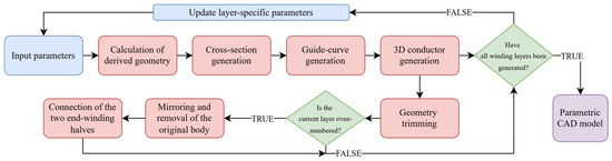
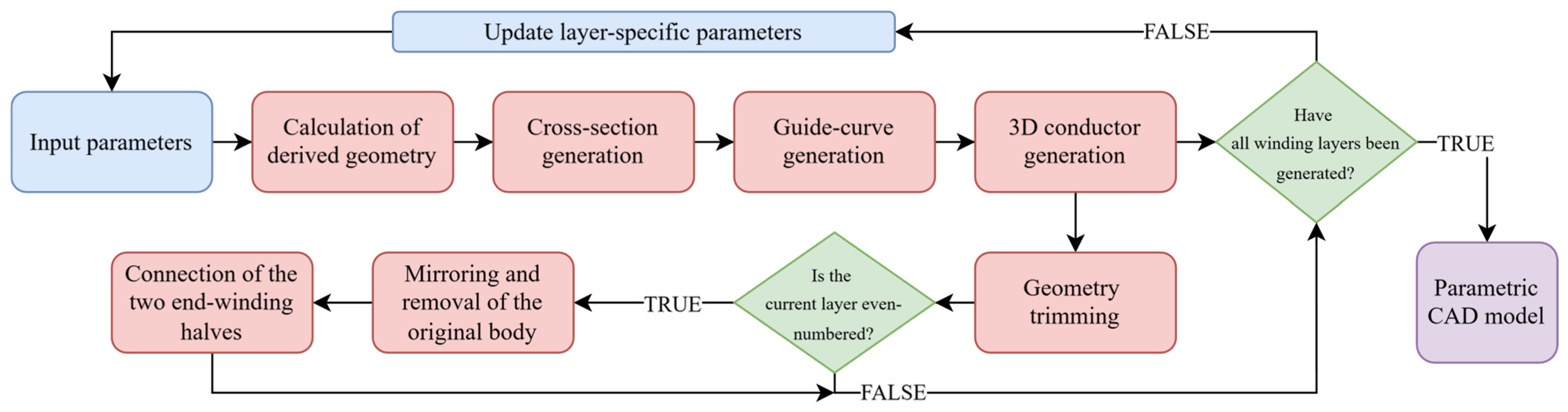
A CAD automation script was developed in Ansys SpaceClaim 2025R2 to generate the parametric hairpin end-winding geometry. The workflow of the CAD automation script is shown in Figure 1. The script uses the input parameters from Table 1 to calculate the required geometric quantities, generate conductor cross-sections and guide curves, create and trim the 3D conductor bodies, and repeat the process for all winding layers. This produces a parametric CAD model that can be quickly modified and used consistently in both the analytical and finite-element thermal models.

Figure 1. Workflow of the CAD automation script.

3.2. FEA Model of Hairpin Winding

The numerical thermal model of the hairpin winding is developed using FEA. The parametrically generated CAD geometry described in Section 3.1 is imported into Ansys Mechanical and used as the basis for a steady-state thermal simulation. The conductor body is defined as copper with thermal conductivity of $380 \mathrm{W}·{\mathrm{m}}^{-1}·{\mathrm{K}}^{-1}$, and internal heat generation is applied to represent the Joule losses in the winding. A mesh-independence study confirmed that an element size of $1 \mathrm{m}\mathrm{m}$ provides sufficient spatial resolution of the curved end-winding geometry while maintaining computational efficiency for repeated parametric calculations.

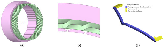
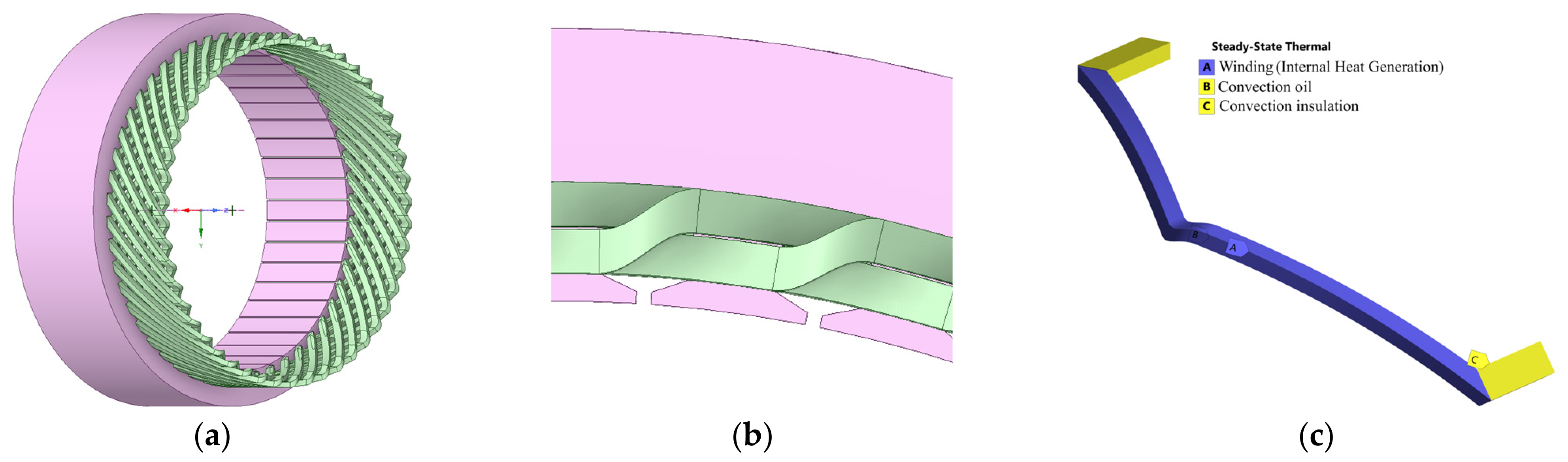
The main steps of the FEA model preparation are summarized in Figure 2. The complete parametrically generated CAD geometry of the hairpin winding with the stator core is shown in Figure 2a, while Figure 2b provides a detailed view of the end-winding region. The corresponding FEA thermal model is shown in Figure 2c, where internal heat generation is assigned to the copper conductor and convection boundary conditions are applied to the oil-cooled and insulation-contact surfaces. For the FEA study, a representative conductor path is extracted from the parametrically generated winding geometry and used for the steady-state thermal calculation. The winding losses, heat-transfer areas, and conductor volume assigned to the representative FEA path are scaled consistently with the corresponding whole-winding quantities used in the analytical model.

Figure 2. FEA model of the hairpin winding: (a) parametrically generated CAD geometry; (b) detail of the end-winding region; and (c) FEA thermal model with applied heat generation and the equivalent insulation/stator side thermal boundary condition.

4. Results and Discussion

This section presents the results obtained from the analytical and FEA thermal models. First, the reference case and the selected parameter ranges are defined. The effects of the main geometrical and cooling parameters on the winding temperature and current density are then evaluated. The analysis focuses on the stator core length, effective oil-cooling correction factor, oil-side heat-transfer coefficient, winding losses, and rotational speed of the oil nozzle. Finally, the analytical predictions are compared with the FEA results to assess the accuracy and applicability of the simplified approach for preliminary design. The results are presented as parametric sensitivity plots enabling rapid current-density estimation.

4.1. Reference Case and Parametric Study Setup

The parametric study is performed to evaluate the influence of selected cooling and geometrical parameters on the winding temperature and current density of the hairpin winding. A reference case is first defined using the input parameters introduced in Section 2.1. The reference winding geometry is based on [17]. The same nominal geometry, material properties, and thermal boundary conditions are used in both models; however, small differences remain between the analytically calculated winding volume and the conductor volume used to define volumetric heat generation in the FEA model. The investigated parameter ranges are summarized in Table 2. In each case, one selected parameter is varied while the remaining parameters are kept at their reference values.

Table 2. Parameter ranges used in the parametric study.

Variable and Unit	Range	Reference Value	Description
$L_{\mathrm{f}\mathrm{e}} \left(\mathrm{m}\mathrm{m}\right)$	20–160	100	Total axial length of the stator core
${\phi }_{\mathrm{o}\mathrm{i}\mathrm{l},\mathrm{e}\mathrm{f}\mathrm{f}} \left(-\right)$	0.1–1.5	1	Effective oil-cooling correction factor applied to the nominal end-winding surface area
$P_{\mathrm{l}\mathrm{o}\mathrm{s}\mathrm{s}} \left(\mathrm{W}\right)$	50–500	150	Winding losses
$n \left(\mathrm{r}\mathrm{p}\mathrm{m}\right)$	100–2900	2500	Rotational speed of the oil nozzle
$h_{\mathrm{o}\mathrm{i}\mathrm{l}} (\mathrm{W}·{\mathrm{m}}^{-2}·{\mathrm{K}}^{-1})$	50–3000	664	Heat-transfer coefficient on the oil-cooled surface

The parameters listed in Table 3 were kept constant throughout the parametric analyses. They define the reference winding geometry, oil-jet conditions, thermal boundary conditions, and material properties, while only the parameter selected for each sensitivity analysis was varied. For the reference values listed in Table 2 and Table 3, the nozzle Reynolds number in (10) is equal to 1509, which lies within the reported validity range. No specific commercial oil was assumed in this study. Instead, a generic cooling oil is represented by the constant thermophysical properties listed in Table 3 at an assumed mean temperature of $30 °\mathrm{C}$.

Table 3. Fixed parameters used in the parametric study.

Parameter and Unit	Value	Description
$h_{\mathrm{s}} \left(\mathrm{m}\mathrm{m}\right)$	3	Height of one rectangular conductor of the hairpin winding
$d_{\mathrm{s}} \left(\mathrm{m}\mathrm{m}\right)$	3	Width of one rectangular conductor of the hairpin winding
$Q_1 \left(-\right)$	48	Total number of stator slots
$Q_{\mathrm{c}} \left(-\right)$	8	Coil pitch expressed as the number of stator slots between two coil sides
$L_{\mathrm{f}\mathrm{e},\mathrm{o}\mathrm{u}\mathrm{t}} \left(\mathrm{m}\mathrm{m}\right)$	5	Length of the straight conductor part protruding from the stator core
$R_{\mathrm{c}} \left(\mathrm{m}\mathrm{m}\right)$	90.87	Mean radius of the end-winding circular path
$L_{\mathrm{k}\mathrm{c}} \left(\mathrm{m}\mathrm{m}\right)$	40	Perpendicular distance from the stator core to the end of the end winding
$d_{\mathrm{j}\mathrm{e}\mathrm{t}} \left(\mathrm{m}\mathrm{m}\right)$	0.9	Nozzle diameter
${\dot{m}}_{\mathrm{j}\mathrm{e}\mathrm{t}} \left(\mathrm{g}·{\mathrm{s}}^{-1}\right)$	3.2	Mass flow rate per nozzle
${\rho }_{\mathrm{o}\mathrm{i}\mathrm{l}} \left(\mathrm{k}\mathrm{g}·{\mathrm{m}}^{-3}\right)$	850	Oil density at the considered oil temperature
${\mu }_{\mathrm{o}\mathrm{i}\mathrm{l}} \left(\mathrm{P}\mathrm{a}·\mathrm{s}\right)$	$3·{10}^{-3}$	Oil dynamic viscosity at the considered oil temperature
${\lambda }_{\mathrm{o}\mathrm{i}\mathrm{l}} (\mathrm{W}·{\mathrm{m}}^{-1}·{\mathrm{K}}^{-1})$	0.13	Oil thermal conductivity at the considered oil temperature
$t_{\mathrm{o}\mathrm{i}\mathrm{l}} \left(°\mathrm{C}\right)$	30	Uniform oil temperature
$t_{\mathrm{i}\mathrm{n}} \left(°\mathrm{C}\right)$	120	Reference temperature on the insulation/stator side
$h_{\mathrm{i}\mathrm{n}} \left(\mathrm{W}·{\mathrm{m}}^{-2}·{\mathrm{K}}^{-1}\right)$	300	Equivalent thermal contact conductance at the winding–stator interface
${\rho }_{\mathrm{e}\mathrm{l},20} \left(\mathsf{\Omega }·\mathrm{m}\right)$	$1.724·{10}^{-8}$	Electrical resistivity of copper at $20 °\mathrm{C}$
${\alpha }_{\mathrm{C}\mathrm{u}} \left({\mathrm{K}}^{-1}\right)$	$3.93·{10}^{-3}$	Temperature coefficient of copper resistivity

4.2. Parametric Influence on Winding Temperature and Current Density

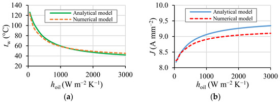
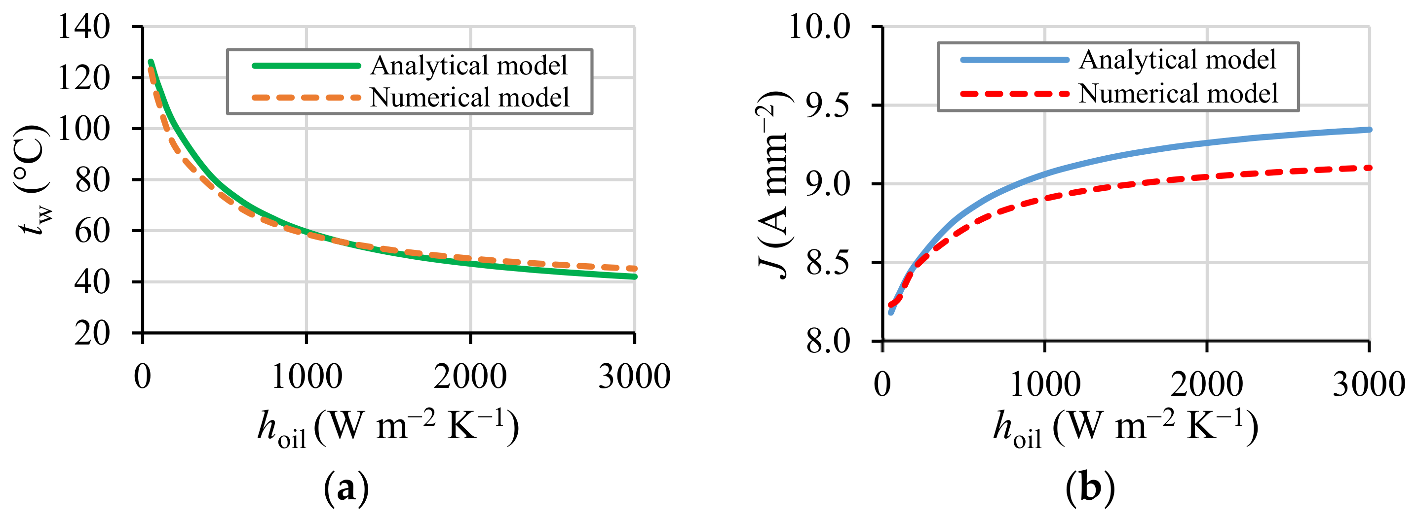
To assess the sensitivity of the results to the assumed oil-side heat-transfer coefficient, $h_{\mathrm{o}\mathrm{i}\mathrm{l}}$ varied from $50$ to $3000 \mathrm{W}·{\mathrm{m}}^{-2}·{\mathrm{K}}^{-1}$, while the remaining parameters were kept at their reference values. As shown in Figure 3, increasing $h_{\mathrm{o}\mathrm{i}\mathrm{l}}$ substantially reduces the average winding temperature, while the current density increases and gradually approaches a plateau. The sensitivity is most pronounced at low HTC values, whereas further increases above approximately $1000 \mathrm{W}·{\mathrm{m}}^{-2}·{\mathrm{K}}^{-1}$ provide a progressively smaller improvement. Both models predict the same trend, although the FEA model yields lower current density values.

Figure 3. Sensitivity of the analytical and FEA predictions to the assumed heat-transfer coefficient on the oil-cooled surface: (a) average winding temperature; (b) current density.

Over the investigated HTC range, the analytical prediction of $J$ increases from approximately $8.0$ to $9.4 \mathrm{A}·{\mathrm{m}\mathrm{m}}^{-2}$, while the FEA prediction reaches approximately $9.1 \mathrm{A}·{\mathrm{m}\mathrm{m}}^{-2}$, indicating that the influence of HTC uncertainty increases as the cooling intensity rises.

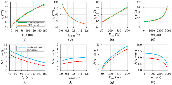
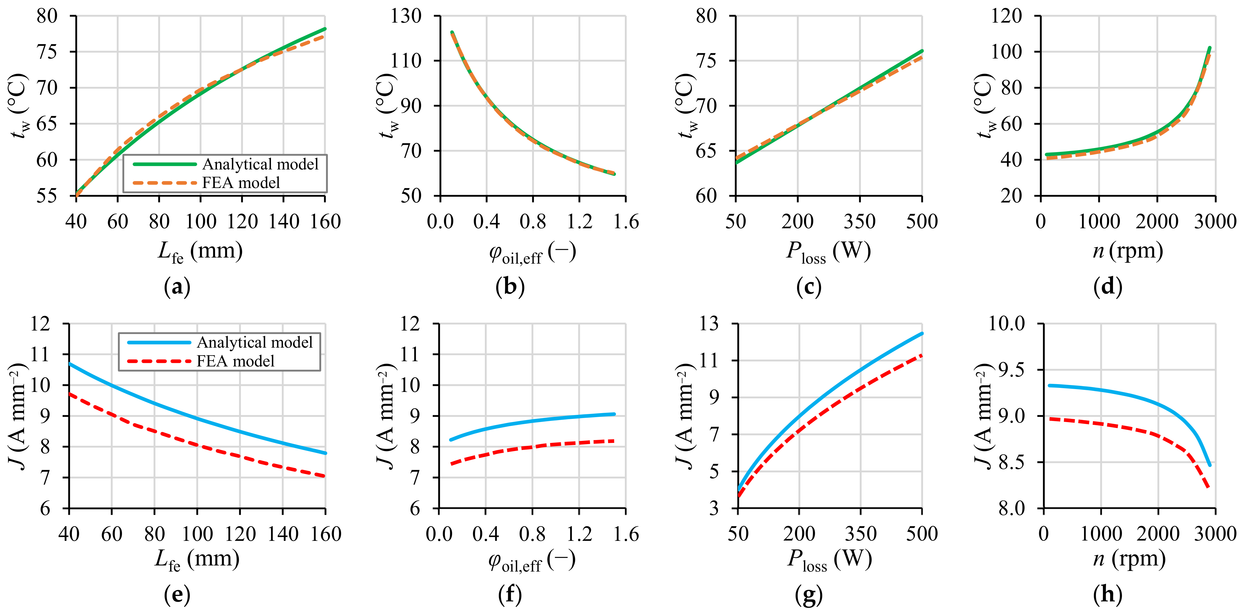
The effects of the remaining geometrical and operating parameters are summarized in Figure 4. Each graph contains the analytical prediction and the corresponding FEA result, which enables a direct comparison of both approaches over the investigated parameter range. The upper row, Figure 4a–d, shows the influence of selected parameters on the average winding temperature $t_{\mathrm{w}}$, while the lower row, Figure 4e–h, presents the corresponding current density $J$. For a consistent comparison, the FEA temperature is evaluated as the average temperature of the copper conductor. For the reference case, the FEA model predicts a volume-averaged winding temperature of $69.2 °\mathrm{C}$ and a maximum local temperature of $86.6 °\mathrm{C}$, resulting in a hot-spot-to-average temperature difference of $17.4 \mathrm{K}$. For a prescribed winding loss $P_{\mathrm{l}\mathrm{o}\mathrm{s}\mathrm{s}}$, an increase in the average winding temperature $t_{\mathrm{w}}$ increases the copper resistivity ${\rho }_{\mathrm{e}\mathrm{l}}\left(t_{\mathrm{w}}\right)$ and therefore reduces the corresponding current density $J$. The winding temperatures predicted by both models agree well, indicating that the analytical heat-balance model captures the main thermal trends of the hairpin winding.

Figure 4. Comparison of analytical and FEA sensitivity results: (a) influence of stator core length on average winding temperature; (b) influence of effective oil-cooling correction factor on average winding temperature; (c) influence of winding losses on average winding temperature; (d) influence of oil-nozzle rotational speed on average winding temperature; (e) influence of stator core length on current density; (f) influence of effective oil-cooling correction factor on current density; (g) influence of winding losses on current density; (h) influence of oil-nozzle rotational speed on current density.

The influence of the stator core length $L_{\mathrm{f}\mathrm{e}}$ is shown in Figure 4a,e. With increasing $L_{\mathrm{f}\mathrm{e}}$, the winding temperature rises nonlinearly due to changes in heat-transfer surfaces and heat-generating volume, while the current density decreases moderately. The effective oil-cooling correction factor ${\phi }_{\mathrm{o}\mathrm{i}\mathrm{l},\mathrm{e}\mathrm{f}\mathrm{f}}$, shown in Figure 4b,f, reduces the winding temperature as the effective cooling area increases. However, its influence on the corresponding current density is relatively limited.

The effect of winding losses $P_{\mathrm{l}\mathrm{o}\mathrm{s}\mathrm{s}}$ is presented in Figure 4c,g. The winding temperature increases almost linearly with $P_{\mathrm{l}\mathrm{o}\mathrm{s}\mathrm{s}}$, as expected for a steady-state thermal model. The influence of oil-nozzle rotational speed $n$ is shown in Figure 4d,h. At a fixed Reynolds number, the applied correlation predicts a decrease in the average Nusselt number with increasing rotational speed. This trend is not solely a mathematical consequence of the fitted correlation but reflects the flow-field behavior observed in the original CFD study [16]. Increasing rotational speed deflects the jet and weakens its direct impingement on the cooled surface, with partial flow separation possible at high speeds. Although rotation can improve the uniformity of oil distribution, the lower average impingement intensity reduces the HTC, increasing the winding temperature and slightly decreasing the corresponding current density.

Although the temperature predictions show good agreement, some deviations are observed in the predicted current density $J$. These deviations are mainly attributed to differences between the winding volume calculated analytically and the conductor volume used to define the volumetric heat generation in the FEA model. Because $J$ is calculated using the considered conductor volume, even small differences in volume affect the resulting values. In addition, differences in the average winding temperature predicted by the analytical and FEA models lead to different temperature-dependent copper resistivities, which further contribute to the deviations in $J$.

The analytical model should be regarded as a design-oriented, reduced-order approximation. The effects of the actual oil distribution and local heat transfer are represented by spatially averaged boundary conditions under steady-state operation. Consequently, the model accuracy may decrease for extreme geometries or strongly non-uniform cooling conditions that lead to pronounced temperature gradients and local hot spots. In such cases, detailed FEA using locally resolved HTC values obtained from CFD analyses or experimental measurements is recommended.

Overall, the analytical model is intended primarily for rapid trend assessment and preliminary sizing within the investigated parameter range, whereas detailed FEA is more appropriate for evaluating local temperatures and verifying hot spots.

5. Conclusions

This study presented a design-oriented workflow combining parametric end-winding geometry, an analytical thermal model, and FEA verification to estimate current density in oil-cooled hairpin windings. The analytical model reproduced the main trends in average winding temperature and is therefore suitable for rapid preliminary sizing. Differences in the predicted current density were mainly attributed to differences in the conductor volumes and average winding temperatures used in the two models. The model applicability is limited by its steady-state formulation, spatially averaged HTC, and simplified representation of the cooled surface. Detailed FEA using spatially resolved HTC data from CFD or measurements is therefore recommended for non-uniform cooling conditions, extreme geometries, and local hot-spot assessment.

Future work will focus on experimental validation using a representative hairpin stator unit under controlled electrical and cooling conditions. The measured steady-state temperatures will be used to evaluate both models.

References

- Gai, Y.; Kimiabeigi, M.; Chuan Chong, Y.; Widmer, J.D.; Deng, X.; Popescu, M.; Goss, J.; Staton, D.A.; Steven, A. Cooling of Automotive Traction Motors: Schemes, Examples, and Computation Methods. IEEE Trans. Ind. Electron. 2019, 66, 1681–1692. [Google Scholar] [CrossRef] [Scilit]
- Gronwald, P.-O.; Kern, T.A. Traction Motor Cooling Systems: A Literature Review and Comparative Study. IEEE Trans. Transp. Electrif. 2021, 7, 2892–2913. [Google Scholar] [CrossRef] [Scilit]
- Nachouane, A.B.; Abdelli, A.; Friedrich, G.; Vivier, S. Numerical Study of Convective Heat Transfer in the End Regions of a Totally Enclosed Permanent Magnet Synchronous Machine. IEEE Trans. Ind. Appl. 2017, 53, 3538–3547. [Google Scholar] [CrossRef] [Scilit]
- Sciascera, C.; Giangrande, P.; Papini, L.; Gerada, C.; Galea, M. Analytical Thermal Model for Fast Stator Winding Temperature Prediction. IEEE Trans. Ind. Electron. 2017, 64, 6116–6126. [Google Scholar] [CrossRef] [Scilit]
- Nuzzo, S.; Barater, D.; Gerada, C.; Vai, P. Hairpin Windings: An Opportunity for Next-Generation E-Motors in Transportation. IEEE Ind. Electron. Mag. 2022, 16, 52–59. [Google Scholar] [CrossRef] [Scilit]
- Berardi, G.; Bianchi, N. Design Guideline of an AC Hairpin Winding. In Proceedings of the 2018 XIII International Conference on Electrical Machines (ICEM), Alexandroupoli, Greece, 3–6 September 2018; pp. 2444–2450. [Google Scholar]
- Bianchi, N.; Berardi, G. Analytical Approach to Design Hairpin Windings in High Performance Electric Vehicle Motors. In Proceedings of the 2018 IEEE Energy Conversion Congress and Exposition (ECCE), Portland, OR, USA, 23–27 September 2018; pp. 4398–4405. [Google Scholar]
- Zhang, F.; Gerada, D.; Xu, Z.; Liu, C.; Zhang, H.; Zou, T.; Chong, Y.C.; Gerada, C. A Thermal Modeling Approach and Experimental Validation for an Oil Spray-Cooled Hairpin Winding Machine. IEEE Trans. Transp. Electrif. 2021, 7, 2914–2926. [Google Scholar] [CrossRef] [Scilit]
- Preci, E.; Nuzzo, S.; Valente, G.; Gerada, D.; Barater, D.; Degano, M.; Buticchi, G.; Gerada, C. Segmented Hairpin Topology for Reduced Losses at High-Frequency Operations. IEEE Trans. Transp. Electrif. 2022, 8, 688–698. [Google Scholar] [CrossRef] [Scilit]
- Shams Ghahfarokhi, P.; Podgornovs, A.; Kallaste, A.; Marques Cardoso, A.J.; Belahcen, A.; Vaimann, T. The Oil Spray Cooling System of Automotive Traction Motors: The State of the Art. IEEE Trans. Transp. Electrif. 2023, 9, 428–451. [Google Scholar] [CrossRef] [Scilit]
- Liu, C.; Xu, Z.; Gerada, D.; Li, J.; Gerada, C.; Chong, Y.C.; Popescu, M.; Goss, J.; Staton, D.; Zhang, H. Experimental Investigation on Oil Spray Cooling with Hairpin Windings. IEEE Trans. Ind. Electron. 2020, 67, 7343–7353. [Google Scholar] [CrossRef] [Scilit]
- Liu, C.; Gerada, D.; Xu, Z.; Chong, Y.C.; Michon, M.; Goss, J.; Li, J.; Gerada, C.; Zhang, H. Estimation of Oil Spray Cooling Heat Transfer Coefficients on Hairpin Windings with Reduced-Parameter Models. IEEE Trans. Transp. Electrif. 2021, 7, 793–803. [Google Scholar] [CrossRef] [Scilit]
- Gai, Y.; Xu, Z.; Liu, C.; Chong, Y.C. Analysis of a Modular LPTN for an Oil-Cooled Hairpin Traction Motor with HTC from CFD. IEEE Trans. Transp. Electrif. 2025, 11, 9145–9154. [Google Scholar] [CrossRef] [Scilit]
- Bergfried, C.; Abdi Qezeljeh, S.; Roisman, I.V.; De Gersem, H.; Hussong, J.; Späck-Leigsnering, Y. Thermal Finite-Element Model of Electric Machine Cooled by Spray. Energies 2025, 18, 84. [Google Scholar] [CrossRef] [Scilit]
- Hruska, K.; Dvorak, P. Calculation of a Lap Winding Coil Geometry. In Mechatronics 2017; Březina, T., Jabłoński, R., Eds.; Advances in Intelligent Systems and Computing; Springer International Publishing: Cham, Switzerland, 2018; Volume 644, pp. 236–247. [Google Scholar]
- Lu, Q.; Parameswaran, S.; Ren, B. Heat Transfer by a Rotating Liquid Jet Impingement Cooling System. In Proceedings of the Volume 8B: Heat Transfer and Thermal Engineering; American Society of Mechanical Engineers: Pittsburgh, PA, USA, 2018; p. V08BT10A026. [Google Scholar]
- Matt, D.; Boubaker, N.; Aitakkache, M.; Enrici, P.; Huselstein, J.-J.; Martire, T. High Power Very Low Voltage Electric Motor for Electric Vehicle. In New Perspectives on Electric Vehicles; Găiceanu, M., Ed.; IntechOpen: London, UK, 2022. [Google Scholar]
Disclaimer/Publisher’s Note: The statements, opinions and data contained in all publications are solely those of the individual author(s) and contributor(s) and not of MDPI and/or the editor(s). MDPI and/or the editor(s) disclaim responsibility for any injury to people or property resulting from any ideas, methods, instructions or products referred to in the content. |
© 2026 by the authors. Licensee MDPI, Basel, Switzerland. This article is an open access article distributed under the terms and conditions of the Creative Commons Attribution (CC BY) license.