


Abstract
Accurate modelling of price formation in electricity markets requires capturing the underlying supply and demand structure rather than predicting scalar prices alone. This structure is based on the participants’ bidding process, who submit energy volume offers in the form of block orders and hybrid curve orders. This work addresses the problem of day-ahead forecasting of aggregated hybrid supply curves in the Greek DAM at a 15 min resolution. A hybrid methodology is proposed that combines FPCA, which reduces the high-dimensional curve space to a small set of latent factors, with gradient-boosted forecasts that recursively use models driven by calendar effects, lagged latent dynamics, and exogenous variables (load, RES, and cross-border capacities). Forecasted curves are reconstructed and refined via band-specific residual correction and feasibility constraints. A baseline FPCA backed by ARIMA residual forecasting is used for comparison. The approach is validated for January–March 2026 using a strict day-ahead setup. Evaluation over selected days between January and March 2026 demonstrates that the proposed methodology generally improves forecasting accuracy and maintains stronger performance under evolving market conditions. Results demonstrate that the proposed framework effectively captures curve dynamics, while emphasising the importance of system-state information under changing conditions.
1. Introduction
1.1. Aggregated Supply Curves in the Electricity Market
Electricity markets operate through complex interactions between supply and demand, where prices emerge from the intersection of bidding curves submitted by market participants aggregated by MTU, regardless of energy-producing technology and type of demand. In the European DAM, including the Greek market, orders submitted by market participants are aggregated and cleared through a centralised algorithm that matches supply and demand to maximise social welfare, as defined within the European market coupling framework [1,2].
In this context, aggregated hybrid supply curves play a central role. Each hybrid curve represents the cumulative offered energy from all energy suppliers as a function of price and reflects the system’s instantaneous marginal cost structure, combining renewable generation, thermal units, and cross-border exchanges. These curves are inherently high-dimensional, monotonic, and time-dependent, and their evolution encapsulates the effects of system conditions such as load demand, renewable penetration, and network constraints. Furthermore, market mechanisms such as block orders introduce non-convexities, shifting the effective supply curve and directly affecting price formation.
1.2. Literature Review
Classical approaches rely on statistical and econometric models, while more recent work employs machine learning techniques. A comprehensive review by Rafał Weron [3] highlights the evolution of these methods and emphasises the inherent difficulty of capturing price spikes, regime changes, and nonlinear dependencies in electricity markets. Structural models explicitly incorporate supply and demand mechanisms, offering improved interpretability and economic consistency [4]. Despite their predictive capability, such models treat price as an isolated variable and do not explicitly account for the structural mechanism of market clearing.
To address this limitation, recent research has explored the use of FDA techniques to high-dimensional temporal forecasting problems, demonstrating that complex curve structures can be efficiently represented through a small number of latent functional components [5,6], enabling the transformation of a complex functional forecasting problem into a multivariate time-series problem. Recent work has also explored direct forecasting of supply and demand curves, such as the X-model proposed by Ziel and Steinert [7], which reconstructs market clearing through the interaction of sale and purchase curves. In particular, FPCA provides an efficient framework for representing time-varying curves in a low-dimensional latent space. Applications of FPCA in energy systems demonstrate its ability to capture dominant modes of variation while preserving the structural properties of the data [8].
However, baseline FPCA-based approaches that rely on complementary linear time-series models, such as ARIMA, for forecasting the latent factors are limited in their ability to capture nonlinear relationships and the influence of exogenous variables. Electricity markets are driven by a wide range of external factors, including load demand, renewable generation, cross-border capacity, and system constraints, which introduce nonlinear and regime-dependent behaviour. This work extends previous research [9], which indicated that incorporating exogenous variables such as load and RES significantly improves forecasting performance, while also highlighting the limitations of purely linear latent dynamics.
Recent advances in machine learning, particularly ensemble methods such as gradient boosting, offer a flexible alternative for modelling nonlinear dependencies and interactions between features [10]. These methods have been successfully applied in forecasting problems where complex relationships between predictors and target variables are present, a frequent occurrence in electricity markets [11].
To address these challenges, this paper proposes a hybrid FPCA–machine learning framework for the day-ahead forecasting of aggregated hybrid supply curves at a 15 min resolution. The methodology combines the structural advantages of FPCA with the predictive flexibility of machine learning. Specifically, FPCA is used to reduce the dimensionality of the curve space, while the resulting latent factors are forecast using gradient boosting models driven by a rich set of features, including calendar effects, lagged dynamics, and exogenous variables such as electricity load, renewable generation, and ATCs between Greece and the surrounding countries, Albania, Italy, Bulgaria, Türkiye, and N. Macedonia. Forecasting is performed in a day-ahead framework, in which the 96 MTUs for a selected delivery day are predicted using only past information, ensuring consistency with real market operations.
2. Materials and Methods
2.1. Data Repositories
For data training, past aggregated hybrid curves that are publicly available from the Greek NEMO, HEnEx S.A., were used. Day-ahead RES and load forecasts, and published ATCs between Greece and the surrounding countries from the Greek TSO, IPTO S.A., were used as features.
2.2. Curve Decomposition with FPCA
In order to forecast the aggregated hybrid supply curves in the Greek DAM at a 15 min MTU resolution, both models subject each curve to decomposition via the FPCA method. The hybrid curves are defined on a fixed price grid and represented as:
where is the cumulative offered volume in MW at the price level , while t indexes time in 15 min intervals. The price grid was derived from the published files that contain the aggregated curve data, resulting in the adoption of a non-uniform, fixed price grid, ranging from −500 EUR/MWh to 4000 EUR/MWh, which are the price lower and upper bounds, according to the DAM Trading Rulebook published by HEnEx. Each curve can be stacked in a single matrix in the form:
Each row is a monotonic non-decreasing function of price, consisting of a set of price-volume points, as published by HEnEx. The forecasting setup is divided into a training set with a rolling window of selected days, a validation step over a certain number of days for hyperparameter selection, and a testing phase, where the forecast is compared with an actual aggregated supply curve.
Both the baseline model and the proposed one share a common process that addresses the multidimensional data, the FPCA method, where the curves are centred by subtracting from each one the mean curve μ:
And Singular Value Decomposition is applied to the centred curves:
The forecasted curves are constructed in the form of
With symbolising the basis curves and the time-varying scores. The process retains K significant terms and forecasts the components. As a condition for the determination of the K terms, the acceptance ratio, ar, is used:
With M symbolising the total k components, and the squared singular values of the Σ component. The deviation between the ML model and the linear baseline model begins at this point, where the scores need to be forecast.
2.3. Linear Score Forecasting with the Baseline Model
The baseline model forecasts each score by using ridge regression for the deterministic part and ARIMA for the residuals. Ridge regression is formulated as
where contains Fourier terms to capture potential periodic behaviours, calendar dummies, and exogenous features of electricity load forecasts, renewable energy generation forecasts, and ATCs with neighbouring countries, published the day before market opening time, as well as their lagged values, with 1, 2, 4, 96, 672 lags.
Residual modelling is performed by implementing ARIMA to capture remaining patterns in the residuals:
Since any trends are expected to be captured by the deterministic component, the backshift operator is neglected, and the parameter search is limited to a (p,q) grid. After this process, the forecasts are evaluated for overfitting using the AIC, while residual whiteness was evaluated using the Ljung–Box test.
2.4. Score Forecasting with Gradient Boosting
2.4.1. Model Description
The ML model is a gradient-boosted regression tree, an LSBoost regression ensemble. Each FPCA score is modelled as an ensemble of 100 weak regression trees:
where M is the total number of trees, η is the learning rate, calibrated equal to 0.05, and is each regression tree. The model is trained sequentially, meaning that each new tree tries to correct the residual errors left by the previous tree:
2.4.2. Feature Selection
The feature vector x contains daily, semi-daily, and weekly Fourier terms, lagged features of market-state features, such as load forecasts, RES forecasts, their subtraction as net load, import/export daily ATCs, and regime-like dummy variables. The lag vector that was used contains 1, 2, 4, 96, 672, taking into account lagged values up to 1 h of the same day, values of the same MTU but previous day, and the same MTU of the week before.
Based on the available data, additional features were produced, such as the aforementioned net load:
Capturing the residual demand that must be covered by thermal generation, hydropower, and imports. To isolate instances when the system is stressed during positive net load, the subtraction’s positive values were stored as a separate feature. Ramping stress and sudden system changes were taken into account by calculating net load ramps and their absolute values:
Another produced feature is the share of RES energy:
This quantifies how dominant renewable energy is at each MTU. The features of net ATC quantify cross-border flexibility:
Therefore, calculating the import/export availability balance, and the total interconnection capacity:
The three-regime dummy variables that were used divide the forecasts into three states: low-price regime, scarcity regime, and neutral regime. The low-price regime is met in MTUs when the renewable energy is substantial, and the net load is relatively small. The scarcity regime is characterized by high net load or large ramp events, while the neutral regime includes any other state:
For the low-price regime, the check conditions include a share of renewables exceeding half of total demand, while net load is compared with its 55th quantile, a relatively relaxed threshold that encompasses both low-net-load and moderately low-load states. In order to register a scarcity regime, the net load needs to surpass the 85th quantile, a state in which the system requires expensive thermal units and imports, or during a sharp increase in the net load. In both cases, the 85th quantile is used to filter the “upper tail” of system stress, avoiding a stricter quantile that would be activated less often.
Instead of an ARIMA residual layer, the boosted trees learn score persistence and nonlinear autoregressive effects by using the score persistence values produced during training as forecast features. In the forecasting phase, the lagged score values 1, 2, 3, 4, 8, 12, 16, 96, 192, and 672 were used for each component k.
2.4.3. Rolling Score Statistics
For rolling windows equal to 4, 16 and 96 (1 h, 4 h and 1 day), the rolling mean is calculated:
The rolling standard deviation is also calculated:
These features assist the model in understanding whether the curve shape has recently been stable or volatile, whether the latent dynamics are trending, or if the current day resembles the previous hours or the previous day.
2.4.4. Band Correction
After the curve construction, a distinct LSBoost is deployed for band correction, aiming to correct systematic curve errors in specific price regions. The band correction process extracts values at selected price grid locations that represent the supply curve geometry. The extractions correspond to the 10th, 20th, 50th, 80th, and 90th quantiles and maximum price level. In addition, local slope indicators are constructed through differences between adjacent quantile points, such as and , that serve as proxies for the steepness of the curves in the low-price and high-price regions, respectively.
For each price column j under correction, a moving average of the curves serves as the baseline curve , which is subtracted from the original , and then the residuals are forecasted:
Resulting in the final curve:
The features that were used were the same for the curve reconstruction, with lags 1, 2, 4, and 96. To ensure that the forecasting model prioritises economically relevant regions of the aggregated supply curve, model selection is performed through a weighted reconstruction loss during validation, which assigns higher importance to specific segments of the curve. For a set of observed curves where t = 1, …, T indexes time and j = 1, …, M indexes the price grid, the loss function is defined as
where symbolises a price-dependent weight. The weight scheme is designed to emphasise the upper price tail, meaning the scarcity region, and the region around the empirical maximum marginal increment of the curve, where the market-clearing zone often occurs.
2.5. Post-Processing for Both Models
To ensure that, at the end of the process, the forecasted curves maintain their expected properties, they are subjected to certain constraints regarding their monotonicity, spike-prevention and physical feasibility. The constraint for non-negative volumes and spike-prevention is ensured by
And the monotonicity:
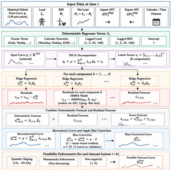
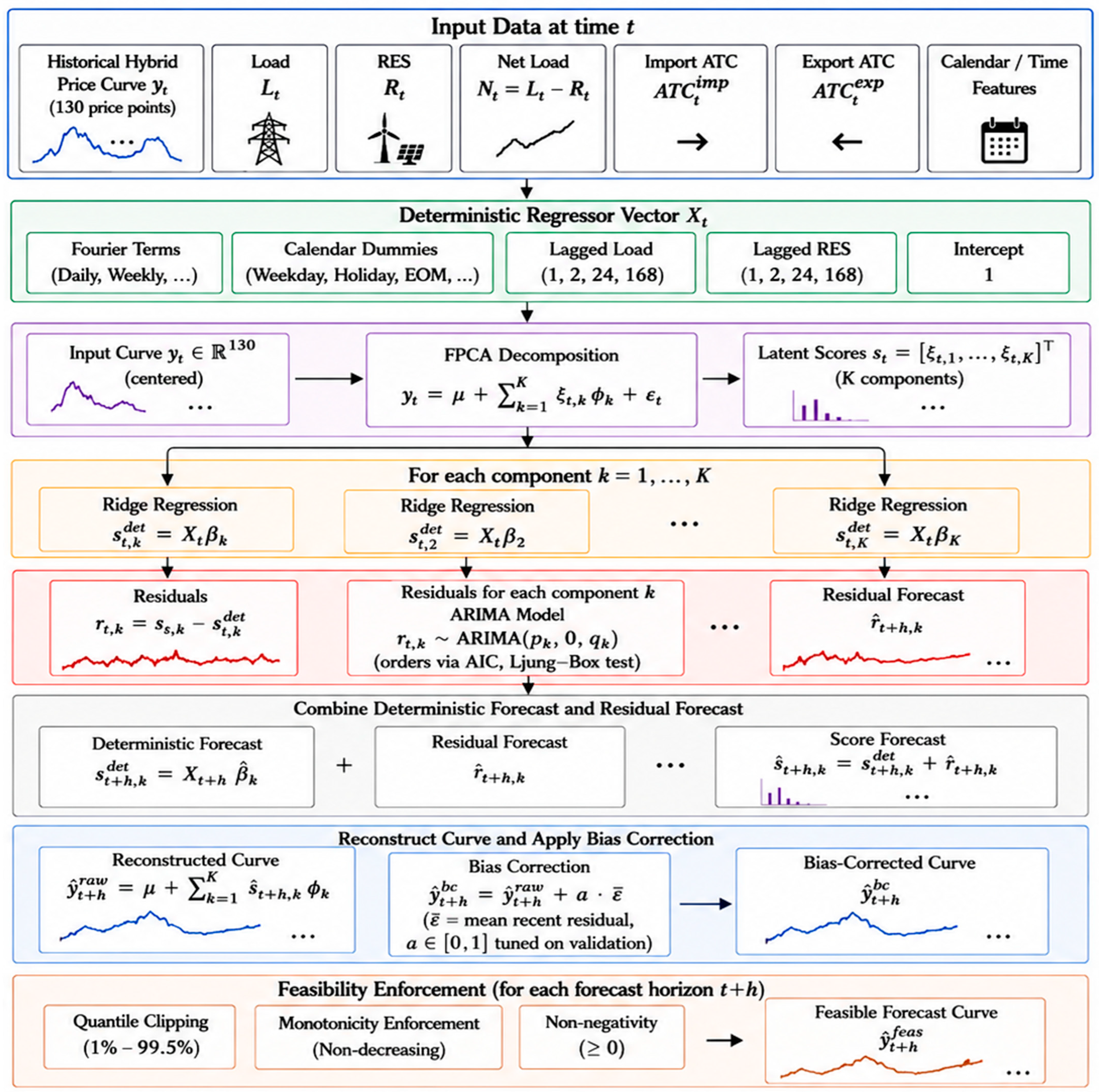
Figure 1 illustrates the overall methodology of the linear model:
Figure 1.
Baseline model methodology.
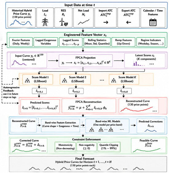
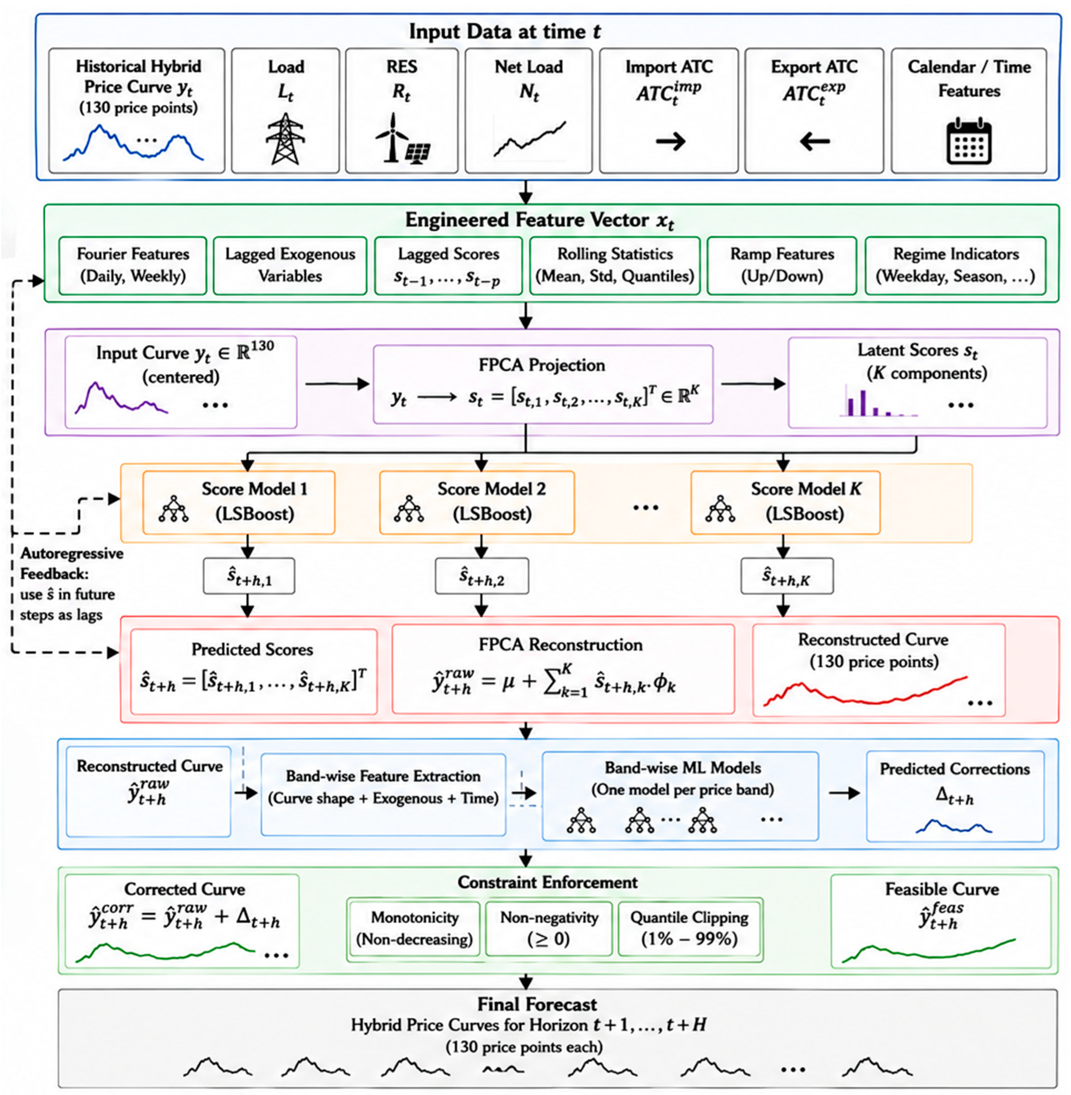
And Figure 2, the ML methodology:
Figure 2.
ML model methodology.
3. Results and Discussion
The two forecasting frameworks were evaluated on seven selected delivery days between January and March 2026. The selected evaluation days were chosen to represent different market conditions observed during the January–March 2026 period, including relatively stable operating conditions, high-renewable low-price periods, scarcity-driven conditions, and regime-transition days. The selected set intentionally includes both successful and failure cases of the proposed methodology in order to evaluate robustness under varying system states. In all cases, the forecasting horizon consisted of the full day-ahead schedule of 96 15 min MTUs, using a rolling 30-day training window split into 2208 sub-training samples and 672 validation samples.
Overall, the proposed ML model outperformed the baseline model in five out of seven test days. The strongest improvements were observed on 31 March, 1 March, 28 February, and 14 February, where the ML model reduced RMSE by approximately 9.6%, 9.7%, 7.7%, and 8.1%, respectively. The improvement was also visible in sMAPE, indicating that the gains were not only due to scale effects but also reflected better relative curve reconstruction. Table 1 summarises the findings for indicative days.
Table 1.
Results for indicative days of January-March 2026.
Excluding the clear failure case of 1 February, the proposed ML model achieved average reductions of approximately 7–8% in MAE, 6–7% in RMSE, and 10–11% in sMAPE (excluding the regime-shift outlier of 1 February) while increasing the average R-squared from 94.7% to 95.0%. This indicates that, under most tested conditions, the nonlinear latent-score model provides a more accurate reconstruction of the full hybrid curve surface, particularly under dynamically evolving market conditions.
The results also show that the FPCA representation remains highly efficient in both models. The baseline retained between 4 and 5 components, explaining approximately 99.55–99.63% of curve variance. The proposed ML model often selected fewer components, usually K = 2 or 3, except on 15 March, where K = 5 was selected. This suggests that the machine-learning score model can extract stronger predictive information from a more compact latent representation, especially when nonlinear exogenous and lagged-score features are informative.
The exception is 1 February 2026, where the ML model performed substantially worse than the baseline, with RMSE increasing from 548.2 MW to 836.6 MW and R-squared falling from 91.5% to 80.2%. This indicates that the ML model is more sensitive to validation misselection or abrupt regime transitions. In that case, the weighted validation loss selected a configuration that did not generalise well to the target day. The baseline model, although less flexible, was more stable because its ridge regression and ARIMA structures impose smoother linear dynamics.
The January result is also informative. On 15 January, both models performed similarly, with the baseline slightly better in MAE, RMSE, and R-squared, while the ML model achieved lower sMAPE. This suggests that when the curve dynamics are relatively regular, the added flexibility of the ML model does not necessarily provide large gains over the baseline.
Overall, the empirical results support the proposed methodology, but with an important qualification: the ML framework improves forecasting accuracy in most cases, particularly in February and March, but it is less robust under certain regime-transition days. Therefore, the proposed model is not uniformly superior but rather a more flexible and generally more accurate framework whose performance depends on stable validation selection and representative recent training data.
4. Conclusions
This paper presented a day-ahead forecasting framework for aggregated hybrid supply curves in the Greek DAM, with a 15 min MTU resolution. Instead of forecasting MCP directly, the proposed approach models the full supply curve as the underlying structural object from which price formation emerges. The methodology combines FPCA-based dimensionality reduction with machine-learning forecasting of latent curve scores, using calendar information, lagged latent dynamics, load, RES, net load, and cross-border ATC variables as inputs. A baseline ridge regression model coupled with ARIMA residual forecasting was used for comparison.
The results show that both approaches can represent hybrid curves efficiently, with a small number of FPCA components explaining more than 99.5% of curve variance. Across the selected test days, the ML framework outperformed the baseline in five out of seven cases, achieving lower MAE, RMSE, and sMAPE and slightly higher R-squared in most February and March evaluations. These findings indicate that nonlinear score forecasting and richer system-state features improve the model’s ability to capture curve dynamics beyond the linear residual structure of the baseline.
However, the results also reveal an important limitation. The proposed ML model underperformed significantly on 1 February 2026, suggesting sensitivity to regime changes, validation misselection, or insufficient representativeness of the recent training window. Therefore, while the ML approach offers improved accuracy and stronger flexibility, the baseline remains more stable under certain conditions.
Future work will focus on improving robustness through adaptive regime detection, direct multi-horizon score forecasting to reduce recursive error propagation, and inclusion of additional supply-side variables such as plant availability, fuel-specific capacity constraints, outages, and block-order forecasts.
Author Contributions
Conceptualization, M.N.; methodology, M.N.; software, M.N.; validation, M.N., T.D. and N.D.; formal analysis, M.N.; investigation, M.N.; resources, E.K.; data curation, M.N.; writing—original draft preparation, M.N. and E.K.; writing—review and editing, M.N., E.K., T.D. and N.D.; visualization, M.N.; supervision, E.K.; project administration, E.K.; funding acquisition, E.K. All authors have read and agreed to the published version of the manuscript.
Funding
This publication is financed by the Project “Strengthening and optimizing the operation of MODY services and academic and research units of the Hellenic Mediterranean University”, with Project ID 80860, funded by the Public Investment Program of the Greek Ministry of Education and Religious Affairs.
Institutional Review Board Statement
Not applicable.
Informed Consent Statement
Not applicable.
Data Availability Statement
The historical aggregated supply curve data is available at the HEnEx website: https://www.enexgroup.gr/web/guest/markets-publications-el-day-ahead-market (accessed on 5 April 2026). The historical electricity load and RES forecasts, as well as import and export ATCs, are available at the Greek TSO’s website: https://www.admie.gr/en/market/market-statistics/detail-data (accessed on 5 April 2026).
Conflicts of Interest
The authors declare no conflicts of interest.
Abbreviations
The following abbreviations are used in this manuscript:
| DAM | Day-Ahead Market |
| FPCA | Functional Principal Component Analysis |
| RES | Renewable Energy Sources |
| ARIMA | Autoregressive Integrated Moving Average |
| MTU | Market Time Unit |
| MCP | Market Clearing Price |
| FDA | Functional Data Analysis |
| ATC | Available Transfer Capacity |
| NEMO | Nominated Energy Market Operator |
| TSO | Transmission System Operator |
| AIC | Akaike Information Criterion |
| MAE | Mean Absolute Error |
| RMSE | Root Mean Squared Error |
| sMAPE | Symmetric Mean Absolute Percentage Error |
| ML | Machine Learning |
References
- Regulation—2015/1222—EN—EUR-Lex. Available online: https://eur-lex.europa.eu/eli/reg/2015/1222/oj/eng (accessed on 28 March 2026).
- Hellenic Energy Exchange S.A. (HEnEx). HEnEx SPOT Trading Rulebook: Day-Ahead and Intra-Day Markets Trading Rulebook; Version 2.5; Hellenic Energy Exchange S.A.: Athens, Greece, 2026. [Google Scholar]
- Weron, R. Electricity Price Forecasting: A Review of the State-of-the-Art with a Look into the Future. Int. J. Forecast. 2014, 30, 1030–1081. [Google Scholar] [CrossRef] [Scilit]
- Carmona, R.; Coulon, M. A Survey of Commodity Markets and Structural Models for Electricity Prices. In Quantitative Energy Finance; Benth, F.E., Kholodnyi, V.A., Laurence, P., Eds.; Springer: New York, NY, USA, 2014; pp. 41–83. [Google Scholar]
- Hyndman, R.J.; Shang, H.L. Forecasting Functional Time Series. J. Korean Stat. Soc. 2009, 38, 199–211. [Google Scholar] [CrossRef] [Scilit]
- Ramsay, J.O.; Silverman, B.W. Functional Data Analysis, 2nd ed.; Springer series in statistics; [Nachdr.]; Springer: New York, NY, USA, 2006. [Google Scholar]
- Ziel, F.; Steinert, R. Electricity Price Forecasting Using Sale and Purchase Curves: The X-Model. Energy Econ. 2016, 59, 435–454. [Google Scholar] [CrossRef] [Scilit]
- Beretta, D.; Grillo, S.; Pigoli, D.; Bionda, E.; Bossi, C.; Tornelli, C. Functional Principal Component Analysis as a Versatile Technique to Understand and Predict the Electric Consumption Patterns. Sustain. Energy Grids Netw. 2020, 21, 100308. [Google Scholar] [CrossRef] [Scilit]
- Nikologiannis, M. Data-Driven Forecasting of Price Formation in the Greek Day-Ahead Electricity Market. Master’s Thesis, Hellenic Mediterranean University, Athens, Greece, 13 March 2026. [Google Scholar] [CrossRef]
- Friedman, J.H. Greedy Function Approximation: A Gradient Boosting Machine. Ann. Stat. 2001, 29, 1189–1232. [Google Scholar] [CrossRef] [Scilit]
- Lago, J.; De Ridder, F.; De Schutter, B. Forecasting Spot Electricity Prices: Deep Learning Approaches and Empirical Comparison of Traditional Algorithms. Appl. Energy 2018, 221, 386–405, Erratum in Appl. Energy 2018, 229, 1286. [Google Scholar] [CrossRef] [Scilit]

Disclaimer/Publisher’s Note: The statements, opinions and data contained in all publications are solely those of the individual author(s) and contributor(s) and not of MDPI and/or the editor(s). MDPI and/or the editor(s) disclaim responsibility for any injury to people or property resulting from any ideas, methods, instructions or products referred to in the content. |
© 2026 by the authors. Licensee MDPI, Basel, Switzerland. This article is an open access article distributed under the terms and conditions of the Creative Commons Attribution (CC BY) license.