Mixed-Integer Nonlinear Programming for Compact-Weight Training of Two-Hidden-Layer Neural Networks ^†

Abstract

We formulate the training of a fully connected feed-forward neural network with two hidden layers as a nonlinear programming framework with integer-parameterized architectures. The upper level selects an L2 regularization coefficient $\lambda \in [{\lambda }_{min},{\lambda }_{max}]$, a learning rate $\alpha \in [{\alpha }_{min},{\alpha }_{max}]$, and admissible hidden widths $(h_1,h_2)\in {\mathbb{N}}^2$ to minimize the compactness-augmented objective $f=\mathrm{BCE}\left(W_N\right)+\gamma {\parallel W_N\parallel }_{\mathrm{F}}^2$, where $W_N={\mathcal{A}}_N(\lambda ,\alpha ;W_0)$ is the deterministic output of N Adam iterations on ${\mathcal{L}}_{\lambda }\left(W\right)=\mathrm{BCE}\left(W\right)+\frac{\lambda }{2}{\parallel \theta \left(W\right)\parallel }_2^2$. The continuous relaxation is solved with projected L-BFGS-B and feasible finite-difference gradients; integer architectures are handled by exhaustive enumeration over a finite set $\mathcal{H}$. We establish: (i) coercivity and attainment of the inner objective for $\lambda >0$ under full-parameter L2 regularization; (ii) attainment of the upper-level problem under lower semi-continuity on the compact hyperparameter box; (iii) conditional KKT accumulation of projected L-BFGS-B under idealized smoothness and vanishing finite-difference assumptions. The framework is validated on five synthetic two-dimensional binary classification benchmarks using the fixed architecture $(48,24)$ to isolate the continuous optimization level. Across the five datasets, the optimized network reaches a Frobenius weight norm $6.4$–$43.7\%$ smaller than the baseline while the classification accuracy gap stays within $-4.0$ to $+0.0$ percentage points. A three-dimensional visualization of the upper-level objective in $({log}_{10}\lambda ,{log}_{10}\alpha )$ reveals a smooth small-$\lambda$ basin and a steep ridge of trivial near-zero weight solutions near the upper regularization bound.

1. Introduction

Two-hidden-layer fully connected neural networks remain canonical models for low-dimensional binary classification, yet their behavior depends sensitively on the L2 regularization coefficient $\lambda$ and the learning rate $\alpha$ [1,2]. In compact-deployment settings, the user also faces discrete architectural choices: selecting hidden widths $(h_1,h_2)\in {\mathbb{N}}^2$ from a finite admissible set and selecting continuous hyperparameters that control accuracy and weight magnitude. We use the term compact-weight training rather than memory-efficient training: with a fixed architecture, the number of stored parameters is unchanged, and the reported compactness is a reduction in the Frobenius norm of the trained weights; structural memory reduction would require the integer level to select a smaller architecture.

Hyperparameter optimization is often treated by black-box methods such as Bayesian optimization and random search [3,4], whereas L-BFGS-B and related quasi-Newton methods provide structured tools for smooth box-constrained nonlinear programs [5,6,7]. This paper connects these viewpoints for a small feed-forward network whose weights are produced by a finite Adam recursion [8]. The continuous relaxation is solved by projected L-BFGS-B with feasible finite-difference gradients, and integer widths are handled by outer enumeration over a finite architectural set $\mathcal{H}$. The implementation is available as a single Python 3.13 module [9].

The contributions are: (i) an explicit mixed-integer nonlinear formulation with an algorithmic inner map $W_N(\lambda ,\alpha )$, rather than an ambiguous nonconvex argmin; (ii) structural results on inner coercivity, upper-level attainment under lower semi-continuity, and conditional KKT accumulation of projected L-BFGS-B; (iii) a fixed-architecture validation on five synthetic datasets showing 6.4–43.7% Frobenius norm reduction with an accuracy gap in $[-4.0,+0.0]$ percentage points; (iv) a surface analysis explaining the role of the upper bound ${\lambda }_{max}$ in avoiding trivial near-zero-weight solutions.

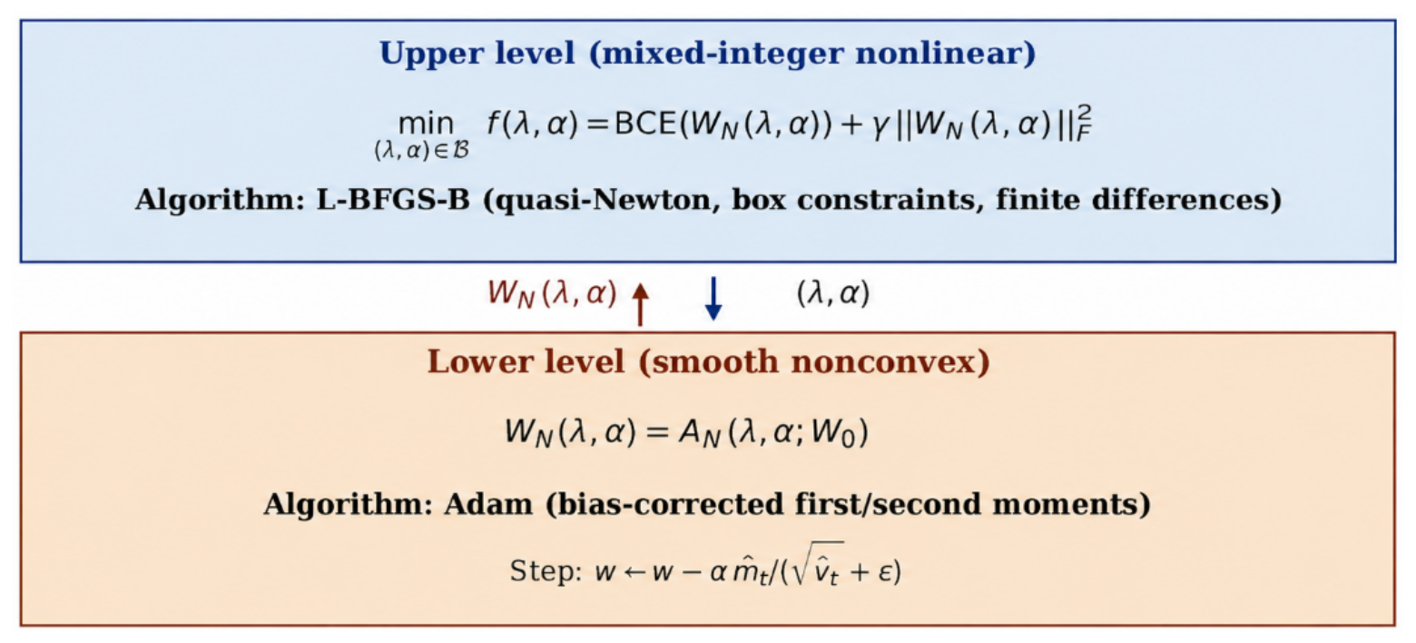
Section 2, Section 3 and Section 4 give the formulation and mathematical analysis, with the algorithmic two-level structure summarized in Figure 1; Section 5 reports the experiments; Section 6 concludes.

Figure 1. Two-level structure of the continuous relaxation $\mathrm{NLP}-{\mathrm{INT}}_c$: L-BFGS-B searches over $(\lambda ,\alpha )\in \mathcal{B}$, while each upper-level objective evaluation calls a finite N-step Adam recursion that returns $W_N(\lambda ,\alpha )$, the network parameters obtained after N Adam iterations from the deterministic initialization $W_0$.

2. Problem Formulation

2.1. Network and Admissible Architectures

Let $X\in {\mathbb{R}}^{m\times 2}$ be a feature matrix of m samples and let $y\in {\{0,1\}}^{m\times 1}$ be the associated binary labels. The classifier is a two-hidden-layer feed-forward network of the form

$$\widehat{y}(x;W)=\sigma \left(\varphi \left(\varphi (x{W}^{\left(1\right)}+b^{\left(1\right)})W^{\left(2\right)}+b^{\left(2\right)}\right)W^{\left(3\right)}+b^{\left(3\right)}\right),$$

(1)

where $\sigma$ is the logistic function and $\varphi$ is a configurable activation, taken as ReLU in all the experiments. The weight matrices are $W^{\left(1\right)}\in {\mathbb{R}}^{2\times h_1}$, $W^{\left(2\right)}\in {\mathbb{R}}^{h_1\times h_2}$, $W^{\left(3\right)}\in {\mathbb{R}}^{h_2\times 1}$, with bias vectors $b^{(\ell )}\in {\mathbb{R}}^{1\times h_{\ell }}$, $\ell =1,2,3$ (where $h_3=1$). The full parameter is

$$W=(W^{\left(1\right)},b^{\left(1\right)},W^{\left(2\right)},b^{\left(2\right)},W^{\left(3\right)},b^{\left(3\right)})\in {\mathbb{R}}^{n(h_1,h_2)},n(h_1,h_2)=3h_1+h_1{h}_2+2h_2+1.$$

(2)

For the purpose of regularization we write $\theta \left(W\right)\in {\mathbb{R}}^{n(h_1,h_2)}$ for the vector that stacks all weight and bias entries of W. The full Euclidean norm of $\theta \left(W\right)$ is then

$${\parallel \theta \left(W\right)\parallel }_2^2={\displaystyle \sum _{\ell =1}^3}\left(\parallel W^{(\ell )}{\parallel }_{\mathrm{F}}^2+{\parallel b^{(\ell )}\parallel }_2^2\right).$$

(3)

We will explicitly distinguish between the full-parameter norm (3), used for regularization and coercivity arguments, and the weight-only Frobenius norm

$${\parallel W\parallel }_{\mathrm{F}}^2=\parallel W^{\left(1\right)}{\parallel }_{\mathrm{F}}^2+\parallel W^{\left(2\right)}{\parallel }_{\mathrm{F}}^2+{\parallel W^{\left(3\right)}\parallel }_{\mathrm{F}}^2,$$

(4)

used as the compactness diagnostic in the upper-level objective and reported in the experimental tables.

The integer hidden widths $(h_1,h_2)$ are constrained to a finite architectural admissible set

$$\mathcal{H}\subset {\mathbb{N}}_{>0}^2,\left|\mathcal{H}\right|<\infty ,$$

(5)

which encodes the discrete decision component of the program. The theoretical formulation and Algorithm 1 apply to any finite admissible set $\mathcal{H}\subset {\mathbb{N}}_{>0}^2$. In the computational validation, we use the singleton set

$${\mathcal{H}}_{\exp }=\left\{(48,24)\right\},$$

(6)

so that the experiments isolate the continuous optimization level in $(\lambda ,\alpha )$ without introducing additional variability from architectural search. A larger architectural set, such as $\left\{\right(16,8),(24,12),(32,16),(48,24),(64,32\left)\right\}$, can be handled by the same outer enumeration in Algorithm 1 but is not used to generate the numerical results reported here.

Algorithm 1 Solver for $\mathsf{NLP}-\mathsf{INT}$: outer enumeration plus inner L-BFGS-B

Require: Data $(X,y)$; admissible set $\mathcal{H}$; box $\mathcal{B}$; weight $\gamma$; inner length $N_{\mathrm{pre}}$. Ensure: Tuple $({\lambda }^{★},{\alpha }^{★},h_1^{★},h_2^{★})$ approximately solving $\mathsf{NLP}-\mathsf{INT}$.   1: Initialize $f^{★}\leftarrow +\infty$.   2: for each $(h_1,h_2)\in \mathcal{H}$ do   3:       Generate deterministic Xavier initialization $W_0(h_1,h_2)$.   4:       Choose an initial point $p_0=({\lambda }_0,{\alpha }_0)\in \mathcal{B}$.   5:       Solve ${min}_{p\in \mathcal{B}}f(p;h_1,h_2)$ with projected L-BFGS-B using the finite-difference gradient (17); obtain $({\lambda }^{†},{\alpha }^{†})$ and value $f^{†}$.   6:       if $f^{†}<f^{★}$ then   7:             $f^{★}\leftarrow f^{†}$; $({\lambda }^{★},{\alpha }^{★},h_1^{★},h_2^{★})\leftarrow ({\lambda }^{†},{\alpha }^{†},h_1,h_2)$.   8:       end if   9: end for 10: return $({\lambda }^{★},{\alpha }^{★},h_1^{★},h_2^{★})$.

2.2. Loss, Regularization and the Compactness Diagnostic

For a fixed architecture $(h_1,h_2)\in \mathcal{H}$, define the binary cross-entropy loss as

$$\mathrm{BCE}\left(W\right)=-{\displaystyle \frac{1}{m}}{\displaystyle \sum _{i=1}^m}\left(y_{i}log\widehat{y}(x_i;W)+(1-y_i)log\left(1-\widehat{y}(x_i;W)\right)\right),$$

(7)

where $\widehat{y}$ is the output in (1); for the theoretical bounds and the numerical implementation, the sigmoid output is clipped to $[{\epsilon }_0,1-{\epsilon }_0]$ with a fixed ${\epsilon }_0\in (0,1/2)$ before evaluating the logarithms. The inner (lower-level) objective combines BCE and L2 regularization on the full parameter $\theta \left(W\right)$:

$${\mathcal{L}}_{\lambda }\left(W\right)=\mathrm{BCE}\left(W\right)+\frac{\lambda }{2}{\parallel \theta \left(W\right)\parallel }_2^2,\lambda \ge 0.$$

(8)

Regularizing the full parameter vector (weights and biases) is the convention required for the coercivity argument of Theorem 1 below; it differs marginally from the bias-free L2 convention of textbook references [1,2], with no practical impact in our experiments since the trained biases remain small relative to the weights.

The upper-level objective penalizes the weight-only Frobenius norm as a compactness diagnostic:

$$f(\lambda ,\alpha ;h_1,h_2)=\mathrm{BCE}\left(W_N(\lambda ,\alpha ;h_1,h_2)\right)+\gamma {\parallel W_N(\lambda ,\alpha ;h_1,h_2)\parallel }_{\mathrm{F}}^2,$$

(9)

where $W_N(\lambda ,\alpha ;h_1,h_2)$ denotes the deterministic output of N Adam iterations on the inner objective ${\mathcal{L}}_{\lambda }$ (defined precisely in Section 3). Because the weight-only norm is the quantity that practitioners customarily monitor for weight compactness, we keep ${\parallel ·\parallel }_{\mathrm{F}}$ rather than ${\parallel \theta (·)\parallel }_2$ in the upper-level penalty; the two coincide up to a small bias contribution in all our experiments.

2.3. The Mixed-Integer Nonlinear Program $\mathsf{NLP}-\mathsf{INT}$

The full problem is

$$\begin{array}{cc}\hfill \mathsf{NLP}-\mathsf{INT}:\underset{(\lambda ,\alpha ,h_1,h_2)}{min}& f(\lambda ,\alpha ;h_1,h_2)\hfill \end{array}$$

(10a)

$$\begin{array}{cc}\hfill \mathrm{s}.\mathrm{t}.& W_N(\lambda ,\alpha ;h_1,h_2)={\mathcal{A}}_N\left(\lambda ,\alpha ;W_0(h_1,h_2)\right),\hfill \end{array}$$

(10b)

$$\begin{array}{cc}\hfill & \lambda \in [{\lambda }_{min},{\lambda }_{max}]=[{10}^{-6},{10}^{-1}],\hfill \end{array}$$

(10c)

$$\begin{array}{cc}\hfill & \alpha \in [{\alpha }_{min},{\alpha }_{max}]=[{10}^{-4},5\times {10}^{-2}],\hfill \end{array}$$

(10d)

$$\begin{array}{cc}\hfill & (h_1,h_2)\in \mathcal{H}\subset {\mathbb{N}}_{>0}^2,\hfill \end{array}$$

(10e)

where ${\mathcal{A}}_N$ denotes N iterations of the Adam recursion applied to ${\mathcal{L}}_{\lambda }$ starting from a deterministic Xavier initialization $W_0(h_1,h_2)$ that depends on the architecture but not on the hyperparameters. The decision variables $(h_1,h_2)$ enter $\mathsf{NLP}-\mathsf{INT}$ both through $\mathcal{H}$ (an integer constraint) and through the dimension $n(h_1,h_2)$ of the weight space; the variables $(\lambda ,\alpha )$ are continuous and box-constrained. The problem is therefore mixed-integer, nonlinear and bilevel. The choice $\gamma >0$ small (we use $\gamma =2\times {10}^{-3}$) keeps classification dominant in (9); the role of $\gamma$ is discussed below.

Remark 1

(Algorithmic vs. variational inner solution). A variational definition $W^{★}\left(\lambda \right)\in {arg\; min}_W{\mathcal{L}}_{\lambda }\left(W\right)$ is unsuitable here because ${\mathcal{L}}_{\lambda }$ is nonconvex and the argmin set need not be single-valued. We therefore define $W_N(\lambda ,\alpha ;h_1,h_2)$ as the deterministic N-step Adam output. This makes the upper objective single-valued, explicitly incorporates the learning rate α, and matches the implementation.

Definition 1

(Continuous relaxation). Fix $(h_1,h_2)\in \mathcal{H}$. The continuous relaxation $\mathsf{NLP}-{\mathsf{INT}}_c(h_1,h_2)$ of $\mathsf{NLP}-\mathsf{INT}$ is obtained by holding the integer pair fixed and minimizing $f(\lambda ,\alpha ;h_1,h_2)$ over the rectangle $\mathcal{B}=[{\lambda }_{min},{\lambda }_{max}]\times [{\alpha }_{min},{\alpha }_{max}]$.

3. Lower-Level Nonconvex Problem and Adam Map

3.1. The Adam Recursion

For fixed hyperparameters $(\lambda ,\alpha )$ and fixed architecture, the lower level is a continuous, piecewise differentiable nonconvex unconstrained problem; under ReLU, gradients are understood in the usual implementation sense, with an arbitrary admissible subgradient selected at kink points. The algorithmic choice in the code is the Adam optimizer [8]. With ${\beta }_1=0.9$, ${\beta }_2=0.999$, $\epsilon ={10}^{-8}$ and bias-corrected first and second moments ${\widehat{m}}_t,{\widehat{v}}_t$, one iteration reads

$$g_t=\nabla {\mathcal{L}}_{\lambda }\left(W_{t-1}\right),{\widehat{m}}_t=\frac{m_t}{1-{\beta }_1^t},{\widehat{v}}_t=\frac{v_t}{1-{\beta }_2^t},W_t=W_{t-1}-\alpha {\widehat{m}}_t\oslash \left(\sqrt{{\widehat{v}}_t}+\epsilon \right),$$

(11)

where $m_t={\beta }_1{m}_{t-1}+(1-{\beta }_1)g_t$, $v_t={\beta }_2{v}_{t-1}+(1-{\beta }_2)g_t\odot g_t$, ⊙ is the Hadamard product and ⊘ is element-wise division. The recursion is initialized with Xavier weights $W_0^{(\ell )}\sim \mathcal{N}(0,2/h_{\ell -1})$ and zero biases, with a fixed random seed so that the initial point depends on $(h_1,h_2)$ but not on $(\lambda ,\alpha )$. We denote the resulting deterministic map of length N by

$$W_N(\lambda ,\alpha ;h_1,h_2)={\mathcal{A}}_N\left(\lambda ,\alpha ;W_0(h_1,h_2)\right),$$

(12)

which is the precise object that enters the upper-level objective (9).

3.2. Existence of Lower-Level Minimizers

Theorem 1

(Inner coercivity and attainment). For every fixed $\lambda >0$ and every architecture $(h_1,h_2)\in {\mathbb{N}}_{>0}^2$, the inner objective ${\mathcal{L}}_{\lambda }:{\mathbb{R}}^{n(h_1,h_2)}\to \mathbb{R}$ defined in (8) is continuous, bounded below, and coercive, namely

$$\underset{{\parallel \theta \left(W\right)\parallel }_2\to \infty }{lim}{\mathcal{L}}_{\lambda }\left(W\right)=+\infty .$$

(13)

Consequently ${\mathcal{L}}_{\lambda }$ attains its infimum on ${\mathbb{R}}^{n(h_1,h_2)}$, and the argmin set ${arg\; min}_W{\mathcal{L}}_{\lambda }\left(W\right)$ is nonempty.

Lemma 1

(BCE is bounded and continuous under output clipping). Let $\widehat{y}(·;W)$ be the clipped sigmoid output $\widehat{y}\in [{\epsilon }_0,1-{\epsilon }_0]$ with ${\epsilon }_0\in (0,\frac{1}{2})$. Then, the BCE map $W\mapsto \mathrm{BCE}\left(W\right)$ in (7) is continuous on ${\mathbb{R}}^{n(h_1,h_2)}$ and satisfies

$$0\le \mathrm{BCE}\left(W\right)\le -log{\epsilon }_0\mathit{for}\mathit{all}W\in {\mathbb{R}}^{n(h_1,h_2)}.$$

(14)

Proof. 

The composition $W\mapsto \widehat{y}(·;W)$ is the composition of finitely many affine maps with the continuous activations $\varphi$ (ReLU) and $\sigma$, projected to $[{\epsilon }_0,1-{\epsilon }_0]$ by the clip; hence, it is continuous in W. For each sample, $-ylog\widehat{y}-(1-y)log(1-\widehat{y})\ge 0$, and, since $\widehat{y}\in [{\epsilon }_0,1-{\epsilon }_0]$, both $log\widehat{y}$ and $log(1-\widehat{y})$ lie in $[log{\epsilon }_0,log(1-{\epsilon }_0)]\subset [log{\epsilon }_0,0]$, so each summand is at most $-log{\epsilon }_0$. Averaging over m samples gives (14). □

Proof of Theorem 1.

By Lemma 1, $\mathrm{BCE}$ is continuous on ${\mathbb{R}}^{n(h_1,h_2)}$ and bounded in $[0,-log{\epsilon }_0]$. The map $W\mapsto \frac{\lambda }{2}{\parallel \theta \left(W\right)\parallel }_2^2$ is continuous, non-negative, and quadratic in the full parameter; in particular, it tends to $+\infty$ as ${\parallel \theta \left(W\right)\parallel }_2\to \infty$ whenever $\lambda >0$. Since $\theta :{\mathbb{R}}^{n(h_1,h_2)}\to {\mathbb{R}}^{n(h_1,h_2)}$ is the identity reshape of the parameter, we have ${\parallel \theta \left(W\right)\parallel }_2^2=\parallel W^{\left(1\right)}{\parallel }_{\mathrm{F}}^2+\parallel b^{\left(1\right)}{\parallel }_2^2+\parallel W^{\left(2\right)}{\parallel }_{\mathrm{F}}^2+\parallel b^{\left(2\right)}{\parallel }_2^2+\parallel W^{\left(3\right)}{\parallel }_{\mathrm{F}}^2+{\parallel b^{\left(3\right)}\parallel }_2^2$, so the regularizer penalizes every entry of W. Adding the two terms reveals that ${\mathcal{L}}_{\lambda }$ is continuous on ${\mathbb{R}}^{n(h_1,h_2)}$, bounded below by 0, and satisfies

$${\mathcal{L}}_{\lambda }\left(W\right)\ge \frac{\lambda }{2}{\parallel \theta \left(W\right)\parallel }_2^2\underset{{\parallel \theta \left(W\right)\parallel }_2\to \infty }{\to }+\infty ,$$

(15)

which is exactly (13). By the Weierstrass theorem [10], the sublevel set $S_0=\{W:{\mathcal{L}}_{\lambda }\left(W\right)\le {\mathcal{L}}_{\lambda }\left(0\right)\}$ is nonempty (it contains 0) and bounded (otherwise, we could extract a sequence $\left\{W_k\right\}\subset S_0$ with $\parallel \theta \left(W_k\right){\parallel }_2\to \infty$, contradicting coercivity), hence becoming compact since it is closed. The continuous function ${\mathcal{L}}_{\lambda }$ attains its infimum on $S_0$, and since any minimizer must satisfy ${\mathcal{L}}_{\lambda }\left(W^{★}\right)\le {\mathcal{L}}_{\lambda }\left(0\right)$, this minimizer is global on ${\mathbb{R}}^{n(h_1,h_2)}$. Therefore, ${arg\; min}_W{\mathcal{L}}_{\lambda }\left(W\right)\ne \varnothing$. □

Remark 2

(Why full-parameter L2 is needed). A bias-free L2 penalty would not be coercive on the full-parameter space: one may set all weight matrices to zero and let a bias vector diverge while the BCE remains bounded by Lemma 1. The full-parameter penalty (8) removes this gap. Numerically, this adjustment is negligible in the reported runs because the trained biases remain small relative to the weights.

Remark 3.

Theorem 1 guarantees the existence but not the uniqueness of a lower-level minimizer: ${\mathcal{L}}_{\lambda }$ is nonconvex in W due to the composition with the activation ϕ, and multiple local minima are routine. The Adam map ${\mathcal{A}}_N$ in (12) is a deterministic surrogate that returns one specific point in the parameter space after N iterations; this surrogate is what enters the upper-level objective, by the convention adopted in Remark 1 and Equation (10b). Throughout we use $N=N_{\mathrm{pre}}=200$ in the L-BFGS-B inner evaluations and $N=1200$ (with early stopping) for the final retraining at the optimized hyperparameters.

3.3. Empirical Lower-Level Convergence

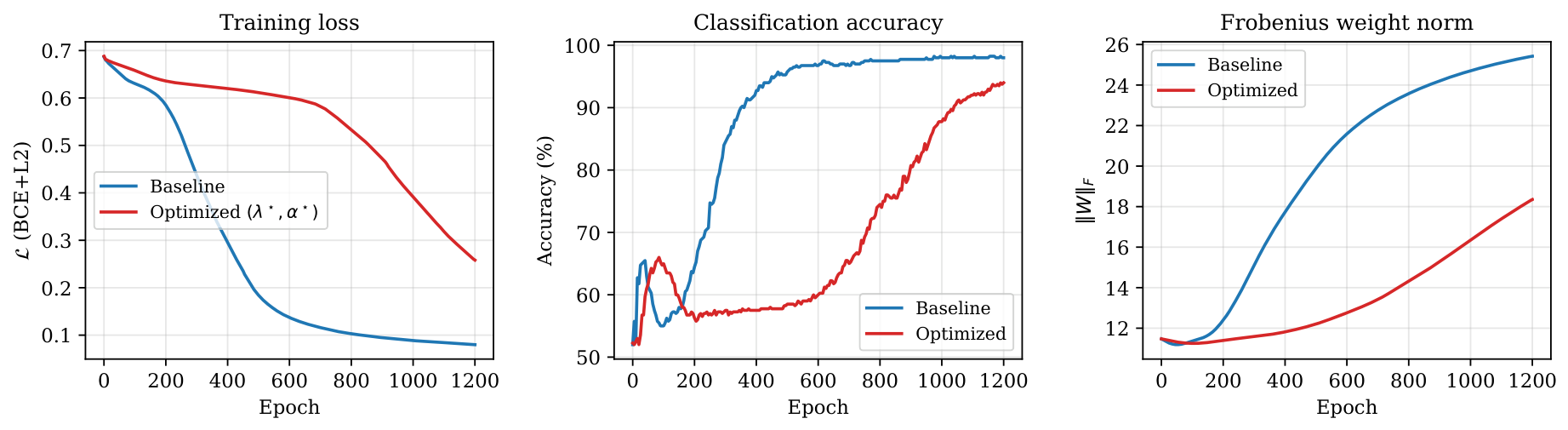
Figure 2 reports the training loss, classification accuracy, and Frobenius norm of $W_t$ on the Spiral dataset for two distinct choices of $(\lambda ,\alpha )$: the unstructured baseline $({\lambda }_{\mathrm{base}},{\alpha }_{\mathrm{base}})=({10}^{-4},3\times {10}^{-3})$ and the L-BFGS-B-tuned pair $({\lambda }^{★},{\alpha }^{★})$ obtained on the same problem. The baseline converges faster in accuracy but reaches a much larger weight norm; the L-BFGS-B-tuned pair drives $\parallel W_t{\parallel }_{\mathrm{F}}$ to a significantly smaller value at the price of a slower-accuracy ramp-up. Both trajectories use early stopping with patience 80 and two learning-rate decays of factor $0.3$, exactly as in the implementation.

Figure 2. Adam trajectory on Spiral for the baseline and L-BFGS-B-tuned hyperparameters. Here, $({\lambda }^{*},{\alpha }^{*})$ denotes the hyperparameter pair returned by the upper-level L-BFGS-B optimization. (left) Training loss ${\mathcal{L}}_{\lambda }$; (centre) accuracy; (right) Frobenius weight norm.

4. Upper-Level Mixed-Integer Nonlinear Program

4.1. Attainment of the Upper-Level Infimum

We now switch to $f(\lambda ,\alpha ;h_1,h_2)$ in (9). Throughout, the inner map $(\lambda ,\alpha )\mapsto W_N(\lambda ,\alpha )$ is the deterministic Adam recursion of length $N_{\mathrm{pre}}=200$ defined in (12), starting from the deterministic Xavier initialization $W_0(h_1,h_2)$.

Theorem 2

(Upper-level attainment under lower semi-continuity). Fix $(h_1,h_2)\in \mathcal{H}$ and the inner recursion parameters $(N_{\mathrm{pre}},{\beta }_1,{\beta }_2,\epsilon ,W_0)$. Assume that the finite-step upper-level objective $f(·,·;h_1,h_2)$ defined in (9) is lower semi-continuous on the compact rectangle $\mathcal{B}$. Then, the continuous relaxation $\mathsf{NLP}-{\mathsf{INT}}_c(h_1,h_2)$ is feasible, f is bounded below by 0, and its infimum is attained on $\mathcal{B}$. If $\mathcal{H}$ is finite and the same lower semi-continuity assumption holds for every $(h_1,h_2)\in \mathcal{H}$, then the full problem $\mathsf{NLP}-\mathsf{INT}$ in (10) admits an optimal $({\lambda }^{★},{\alpha }^{★},h_1^{★},h_2^{★})$.

Proof. 

The rectangle $\mathcal{B}=[{\lambda }_{min},{\lambda }_{max}]\times [{\alpha }_{min},{\alpha }_{max}]$ is nonempty and compact. The point $({\lambda }_{\mathrm{base}},{\alpha }_{\mathrm{base}})\in \mathcal{B}$ is feasible, so $\mathsf{NLP}-{\mathsf{INT}}_c(h_1,h_2)$ is feasible. Since $\mathrm{BCE}\ge 0$ and $\gamma \parallel W_N{\parallel }_{\mathrm{F}}^2\ge 0$, the upper-level objective satisfies $f\ge 0$ on $\mathcal{B}$. By assumption, f is lower semi-continuous on the compact set $\mathcal{B}$; therefore, by the Weierstrass extreme-value theorem for lower semi-continuous functions on compact sets [10], f attains its infimum on $\mathcal{B}$. If $\mathcal{H}$ is finite, the collection of architecture-wise minima $\{{min}_{(\lambda ,\alpha )\in \mathcal{B}}f(\lambda ,\alpha ;h_1,h_2):(h_1,h_2)\in \mathcal{H}\}$ is finite and nonempty. Thus, its minimum is attained by enumeration. This gives an optimal tuple for $\mathsf{NLP}-\mathsf{INT}$. □

Remark 4

(Regularity of the finite-step objective). The lower semi-continuity assumption in Theorem 2 is deliberately stated explicitly. It is automatic if the activation used in the inner recursion is smooth, such as softplus, and if the training schedule is fixed for exactly $N_{\mathrm{pre}}$ steps. In the implementation reported here, the activation is ReLU, the sigmoid output is clipped, and the L-BFGS-B objective evaluation uses a fixed finite Adam budget. This produces a piecewise smooth objective in practice, but it is safer mathematically to state upper-level attainment as a conditional structural result rather than to claim unconditional smoothness for a ReLU-trained bilevel map.

Remark 5

(Boundedness below). A more quantitative lower bound is available: since $\mathrm{BCE}\ge 0$ everywhere and $\gamma \parallel W_N{\parallel }_{\mathrm{F}}^2\ge 0$, we have $f\ge 0$ on $\mathcal{B}$. The infimum is therefore in $[0,f({\lambda }_{\mathrm{base}},{\alpha }_{\mathrm{base}})]$.

4.2. Projected L-BFGS-B with Finite-Difference Gradient

The upper-level relaxation (10a)–(10d) is solved with the projected quasi-Newton L-BFGS-B method [5,6]. At iterate $p_k=({\lambda }_k,{\alpha }_k)\in \mathcal{B}$, the algorithm produces a search direction

$$d_k=-{\widehat{H}}_k^{-1}\widehat{\nabla }f\left(p_k\right),$$

(16)

where ${\widehat{H}}_k^{-1}$ is the L-BFGS limited-memory inverse-Hessian approximation built from the last $\le 10$ pairs of curvature information $(s_i,y_i)=(p_{i+1}-p_i,\widehat{\nabla }f\left(p_{i+1}\right)-\widehat{\nabla }f\left(p_i\right))$, and $\widehat{\nabla }f$ is computed with feasible one-sided finite differences inside the box:

$$\widehat{\nabla }f{\left(p\right)}_j={\displaystyle \frac{f(p+h_j\left(p\right)e_j)-f\left(p\right)}{h_j\left(p\right)}},h_j\left(p\right)=\left\{\begin{array}{cc}\delta ,\hfill & p_j+\delta \le u_j,\hfill \\ -\delta ,\hfill & p_j+\delta >u_j,\hfill \end{array}\right.j=1,2,\delta ={\delta }_k>0,$$

(17)

where $\mathcal{B}=[{\ell }_1,u_1]\times [{\ell }_2,u_2]$. For sufficiently small ${\delta }_k$ (and, in particular, for the value used in the computations), the perturbed point $p+h_j\left(p\right)e_j$ remains feasible for all $p\in \mathcal{B}$. The direction is projected onto $\mathcal{B}$ to maintain feasibility, the step length is chosen by Armijo–Wolfe line search, and the iteration is terminated when $\parallel P_{\mathcal{B}}(p_k-\widehat{\nabla }f\left(p_k\right))-p_k{\parallel }_2<\mathrm{ftol}$ with $\mathrm{ftol}={10}^{-8}$ or after 40 outer iterations.

4.3. Conditional KKT Accumulation Statement

For the box-constrained relaxation $\mathsf{NLP}-{\mathsf{INT}}_c(h_1,h_2)$ the Karush–Kuhn–Tucker conditions at a point $p^{★}=({\lambda }^{★},{\alpha }^{★})\in \mathcal{B}$ read

$$p^{★}=P_{\mathcal{B}}\left(p^{★}-\nabla f\left(p^{★}\right)\right),$$

(18)

where $P_{\mathcal{B}}$ is the Euclidean projection onto the rectangle $\mathcal{B}$. Equation (18) is the standard fixed-point characterization of a stationary point of a continuously differentiable function over a closed convex set [10].

Because the bilevel objective f defined in (9) arises from a $N_{\mathrm{pre}}$-step Adam recursion through a ReLU network—and is therefore at best Lipschitz continuous on $\mathcal{B}$, with a measure-zero set of nondifferentiability inherited from the ReLU breakpoints—we phrase the convergence statement of projected L-BFGS-B as a conditional proposition under explicit idealized hypotheses, rather than as an unconditional theorem.

Proposition 1

(Conditional KKT accumulation of projected L-BFGS-B). Assume that:

(H1) 

The bilevel objective f admits a continuously differentiable extension on the closed rectangle $\mathcal{B}$, i.e., $f\in C^1\left(\mathcal{B}\right)$;

(H2) 

The forward finite-difference step $\delta ={\delta }_k$ in (17) is driven to zero along a subsequence, ${\delta }_k\to 0^{+}$;

(H3) 

The Armijo–Wolfe line search is well-defined at every iterate and satisfies sufficient decrease;

(H4) 

The L-BFGS curvature pairs $(s_i,y_i)$ satisfy the positive-curvature condition $⟨s_i,y_i⟩>0$.

Then, every accumulation point $p^{\infty }$ of the sequence $\left\{p_k\right\}$ produced by the projected L-BFGS-B iteration (16) satisfies the KKT condition (18), i.e., $p^{\infty }$ is a stationary point of the continuous relaxation $\mathsf{NLP}-{\mathsf{INT}}_c(h_1,h_2)$. The convergence is to a KKT point, not necessarily to a global minimum, since f is nonconvex on $\mathcal{B}$.

Proof sketch.

Under (H1)–(H4), the claim is a particularization of the convergence theorem of Byrd–Lu–Nocedal–Zhu for L-BFGS-B [5] (Theorem 6.3), [6] (Section 3). The cited result assumes continuous differentiability of the objective on the feasible box (provided by (H1)), the positive-curvature condition (provided by (H4)), and a step length chosen by Armijo–Wolfe to enforce sufficient decrease (provided by (H3)). The only additional ingredient here is the use of a finite-difference gradient (17) instead of an analytic gradient. By the mean value theorem applied component-wise, $\widehat{\nabla }f{\left(p\right)}_j={\partial }_{j}f\left({\xi }_{p,j}\right)$ for some ${\xi }_{p,j}$ on the feasible segment joining p and $p+h_j\left(p\right)e_j$; under (H1), the partial derivatives are continuous on the compact $\mathcal{B}$ and hence uniformly continuous, so (H2) yields $\widehat{\nabla }f\left(p\right)\to \nabla f\left(p\right)$ uniformly on $\mathcal{B}$ as $|h_j\left(p\right)|\to 0$, and the conclusion of the cited theorem applies on the limit. Compactness of $\mathcal{B}$ guarantees the existence of accumulation points. □

Remark 6

(Gap between theory and implementation). The implementation does not satisfy all idealized hypotheses of Proposition 1: ReLU makes f piecewise smooth rather than globally $C^1$, and SciPy uses a fixed finite-difference step $\delta ={10}^{-5}$ rather than ${\delta }_k\to 0$ [11]. Early stopping and learning-rate decay are used only for final post-optimization training curves, not inside the finite-step objective evaluated by L-BFGS-B. Thus, the proposition is a structural justification of the pipeline, while the computed iterate should be interpreted as an approximate KKT point affected by finite-difference and non-smoothness residuals.

4.4. Integer Enumeration over Architectures

The integer pair $(h_1,h_2)\in \mathcal{H}$ is handled by an outer enumeration: for every $(h_1,h_2)\in \mathcal{H}$, the continuous relaxation $\mathsf{NLP}-{\mathsf{INT}}_c(h_1,h_2)$ is solved by Algorithm 1 and the best value is reported. Since $\mathcal{H}$ is finite, the enumeration is exhaustive and finite-time. In the numerical study below we set $\mathcal{H}={\mathcal{H}}_{\exp }=\left\{(48,24)\right\}$, so the enumeration contains one architecture and the reported empirical effect comes from the continuous L-BFGS-B level. This conservative choice avoids claiming architecture-search results that were not generated, while preserving the mixed-integer formulation and the exact algorithm needed for larger finite architectural sets.

The inner cost of evaluating $f(p;h_1,h_2)$ is one Adam recursion of length $N_{\mathrm{pre}}$, which is $O(N_{\mathrm{pre}}·m·n(h_1,h_2))$ floating-point operations. The total cost of Algorithm 1 is therefore $O\left(\left|\mathcal{H}\right|·K_{\mathrm{LBFGSB}}·N_{\mathrm{pre}}·m·{max}_{(h_1,h_2)\in \mathcal{H}}n(h_1,h_2)\right)$, where $K_{\mathrm{LBFGSB}}$ is the number of inner evaluations of f that L-BFGS-B performs.

5. Experimental Results

5.1. Experimental Setup

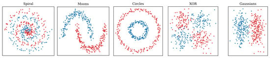
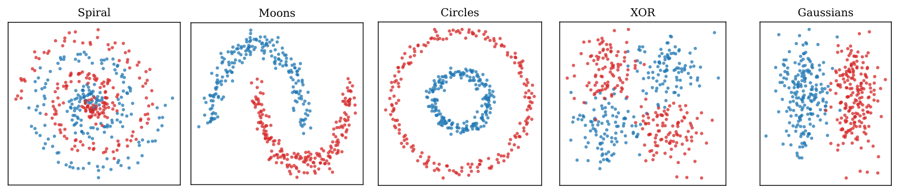
We instantiate Algorithm 1 on the five synthetic two-dimensional balanced binary classification datasets shown in Figure 3: Spiral, Moons, Circles, XOR and Gaussians. Each dataset contains $m=400$ samples, is standardized component-wise, and is generated with a fixed random seed for reproducibility. The reported experiments use the fixed architectural admissible set ${\mathcal{H}}_{\exp }=\left\{(48,24)\right\}$, so both the baseline and optimized networks have the same structural parameter count $n(48,24)=1345$. We set $\gamma =2\times {10}^{-3}$ in (9), $N_{\mathrm{pre}}=200$ for the inner Adam pre-training, a full training horizon of 1200 epochs with early stopping patience 80, and use the ReLU activation. All computations were carried out with the script accompanying this paper [9].

Figure 3. Five synthetic two-dimensional balanced binary classification benchmarks used in the experiments; each dataset contains 400 standardized points. Blue and red points represent the two binary classes.

For each dataset we compare two trained networks:

• The baseline, trained at the canonical unstructured hyperparameters $({\lambda }_{\mathrm{base}},{\alpha }_{\mathrm{base}})=({10}^{-4},3\times {10}^{-3})$ on the fixed architecture $(48,24)$;
• The optimized network, trained at the pair $({\lambda }^{★},{\alpha }^{★})$ returned by Algorithm 1 for the same fixed architecture $(48,24)$.

Both networks share the architecture, seed, training horizon and early stopping policy; they differ only in the continuous hyperparameters $(\lambda ,\alpha )$.

5.1.1. Determinism of the Training Pipeline

The entire pipeline is fully deterministic. Gradients are evaluated in full-batch mode over all $m=400$ samples, with no mini-batch sampling, no inter-epoch data shuffling, and no stochastic augmentation; the Adam recursion (11) is a deterministic map; the Xavier initialization and the dataset generator are each driven by a fixed random seed; and all computations are carried out on CPU in double precision with NumPy/SciPy [11], without nondeterministic GPU kernels. Consequently, for a fixed $(\lambda ,\alpha )$ and architecture, the trained weights $W_N$ are reproduced bit-for-bit across independent executions, so every quantity in Table 1 is an exact value rather than a sample mean. We verified this explicitly: repeating each run yielded differences of exactly 0 (machine-zero) in both classification accuracy and Frobenius norm, so reporting the mean and standard deviation over independent runs would give a degenerate zero standard deviation. Run-to-run variability therefore does not affect the single-point values reported in Table 1.

Table 1. Quantitative comparison of the baseline network and the network trained at the L-BFGS-B-optimized hyperparameters across the five synthetic benchmarks. Architecture $(h_1,h_2)=(48,24)$, parameter count $n=1345$, $\gamma =2\times {10}^{-3}$, and inner Adam steps for L-BFGS-B evaluation $N_{\mathrm{pre}}=200$.

Dataset	${\mathit{\lambda }}^{\mathbf{★}}$	${\mathit{\alpha }}^{\mathbf{★}}$	Acc. Base	Acc. Opt.	${\parallel \mathit{W}\parallel }_{\mathbf{F}}$ Red.	L-BFGS-B Evals
Spiral	$9.81\times {10}^{-5}$	$9.84\times {10}^{-4}$	$98.0\%$	$94.0\%$	$27.8\%$	195
Moons	$1.11\times {10}^{-3}$	$3.69\times {10}^{-2}$	$100.0\%$	$100.0\%$	$43.7\%$	246
Circles	$2.71\times {10}^{-3}$	$3.33\times {10}^{-2}$	$100.0\%$	$100.0\%$	$43.4\%$	309
XOR	$1.00\times {10}^{-4}$	$1.00\times {10}^{-3}$	$97.0\%$	$96.0\%$	$27.2\%$	93
Gaussians	$9.95\times {10}^{-5}$	$1.20\times {10}^{-3}$	$99.8\%$	$99.5\%$	$6.4\%$	156

^★ denotes the hyperparameter values returned by the upper-level L-BFGS-B optimization.

5.1.2. Choice of the Baseline Hyperparameters

The pair $({\lambda }_{\mathrm{base}},{\alpha }_{\mathrm{base}})=({10}^{-4},3\times {10}^{-3})$ is a conventional default operating point rather than a value tuned in our favor. The learning rate is of the order of the canonical Adam default $\alpha ={10}^{-3}$ [8], and $\lambda ={10}^{-4}$ is a standard weak L2 regularization strength for feed-forward classifiers [1,2]. To confirm that this point is representative rather than a deliberately weak reference, we evaluated a coarse $4\times 4$ grid of $(\lambda ,\alpha )$ values around it on the Spiral dataset under the identical training protocol: the baseline attains $98.0\%$ and lies inside a broad high-accuracy plateau (accuracy $\ge 96\%$ for all $\lambda \le {10}^{-3}$ and $\alpha \in [3\times {10}^{-3},3\times {10}^{-2}]$). The reductions in Table 1 therefore cannot be attributed to an artificially poor baseline, since the comparison point is itself accuracy-competitive.

5.2. Quantitative Results: Accuracy and Weight Norm

The principal quantitative results are collected in Table 1. The optimized network achieves a Frobenius weight norm $\parallel W^{★}{\parallel }_{\mathrm{F}}$ that is between $6.4\%$ and $43.7\%$ smaller than that of the unstructured baseline. Because the architecture is fixed at $(48,24)$ in both conditions, this reduction should be interpreted as compact-weight training rather than as a reduction in structural memory footprint. The classification accuracy is preserved exactly on Moons and Circles, remains within $0.3$ percentage points on Gaussians, drops by $1.0$ percentage point on XOR, and degrades by $4.0$ percentage points on the harder Spiral dataset. These results jointly confirm the intuition behind the formulation: the L-BFGS-B level systematically discovers a regularization–learning rate pair that compresses the weight vector at a moderate or null accuracy cost.

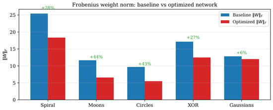
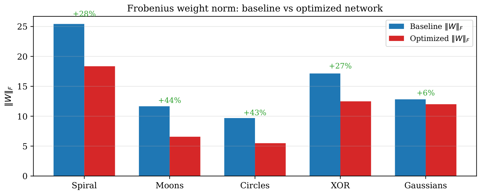
A complementary view of the same results is given in Figure 4: the absolute Frobenius norm of the weight vector drops for every dataset, with the largest gains on the well-separated Moons and Circles (43–$44\%$ reduction) and the smallest on the already-easy Gaussians ($6\%$, on which the baseline norm is already moderate).

Figure 4. Frobenius weight norm before and after L-BFGS-B-based hyperparameter optimization. Annotations report relative reduction.

5.3. Scope of the Integer Level in the Present Experiments

The formulation in (10) and Algorithm 1 are mixed-integer because $(h_1,h_2)$ may be selected from any finite architectural admissible set $\mathcal{H}$. The numerical study in this proceeding paper deliberately uses the singleton set ${\mathcal{H}}_{\exp }=\left\{(48,24)\right\}$, so the empirical results in Table 1 validate the continuous L-BFGS-B level rather than a full multi-architecture search. This distinction is important: the reduction reported in Table 1 is a reduction in the Frobenius norm of the trained weights, not a reduction in the number of stored parameters. A genuine structural memory comparison would require running Algorithm 1 on a larger set such as $\left\{\right(16,8),(24,12),(32,16),(48,24),(64,32\left)\right\}$ and reporting the selected architecture and parameter count for each dataset; this is retained as a direct extension of the present framework.

5.4. Convergence of the Upper-Level Optimizer

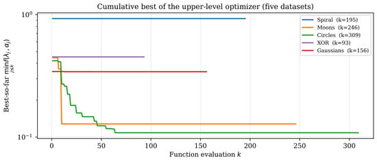
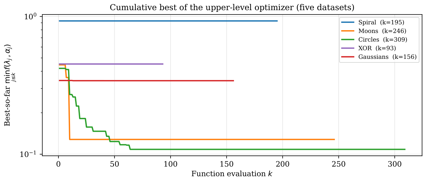
Figure 5 shows the cumulative best-so-far value ${min}_{j\le k}f({\lambda }_j,{\alpha }_j)$ of the L-BFGS-B iteration on each dataset. The Moons and Circles benchmarks exhibit fast monotone descent reaching a numerical plateau within the first ∼20 evaluations; the Spiral, XOR and Gaussians benchmarks reach the plateau more slowly, with the descent profile reflecting the geometry of f on each dataset (cf. Figure 6). The number of inner evaluations $K_{\mathrm{LBFGSB}}$ ranges from 93 (XOR) to 309 (Circles), well within the maximum budget of 40 outer iterations.

Figure 5. Cumulative best-so-far value of the upper-level L-BFGS-B optimizer. Each function evaluation costs one Adam recursion of length $N_{\mathrm{pre}}=200$.

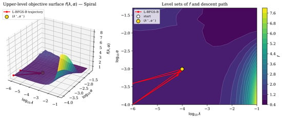
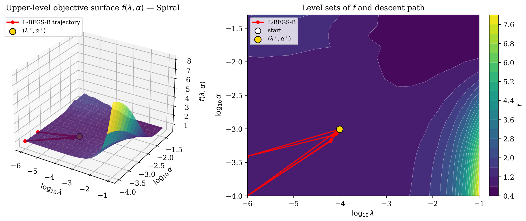
Figure 6. Upper-level objective surface $f(\lambda ,\alpha )$ on Spiral at $(h_1,h_2)=(48,24)$. (Left) 3D view with L-BFGS-B path and optimum. (Right) Level sets and projected path; the small-$\lambda$ basin contrasts with the sharp near-zero weight ridge close to ${\lambda }_{max}$.

5.5. Three-Dimensional Structure of the Upper-Level Objective

To understand the geometric reason for the success of the L-BFGS-B step, we evaluate $f(\lambda ,\alpha )$ on a regular $18\times 18$ logarithmic grid over $\mathcal{B}$ for the Spiral dataset at the fixed architecture $(h_1,h_2)=(48,24)$, with ${log}_{10}\lambda$ ranging over $[-6,-1]$ and ${log}_{10}\alpha$ over $[-4,{log}_{10}\left(0.05\right)]$. Each grid point costs one Adam recursion of length $N_{\mathrm{pre}}$. Figure 6 renders the resulting surface and level sets with the L-BFGS-B path. The surface exhibits: a smooth small-$\lambda$ basin (${log}_{10}\lambda \lesssim -3$) where L-BFGS-B settles; a steep near-zero weight ridge close to ${\lambda }_{max}$, where the classifier approaches chance performance ($\mathrm{BCE}\to -log0.5\approx 0.693$) and the objective is driven mainly by the compactness term; and a descent path that remains in the useful basin instead of entering the trivial ridge. Thus, the upper bound ${\lambda }_{max}={10}^{-1}$ is not cosmetic: it prevents the search from being dominated by excessively regularized near-zero weight solutions.

The shape of f in Figure 6 explains a structural calibration choice that motivated the bounds in (10c) and (10d): the lower bound ${\lambda }_{min}={10}^{-6}$ prevents the formulation from degenerating into the unregularized case where ${\parallel \theta \left(W\right)\parallel }_2\to \infty$ becomes admissible, and the upper bound ${\lambda }_{max}={10}^{-1}$ keeps this near-zero-weight ridge from expanding into increasingly over-regularized regimes. Similarly, $\alpha \in [{10}^{-4},5\times {10}^{-2}]$ excludes both pathologically slow inner trajectories ($\alpha \to 0$) and Adam-divergent regimes ($\alpha$ too large). Together, the four box constraints define a compact closed convex region in which Algorithm 1 is well-posed; under the lower-semicontinuity hypothesis of Theorem 2, an optimum is attained inside this region.

5.6. Decision-Boundary Inspection

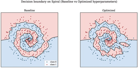
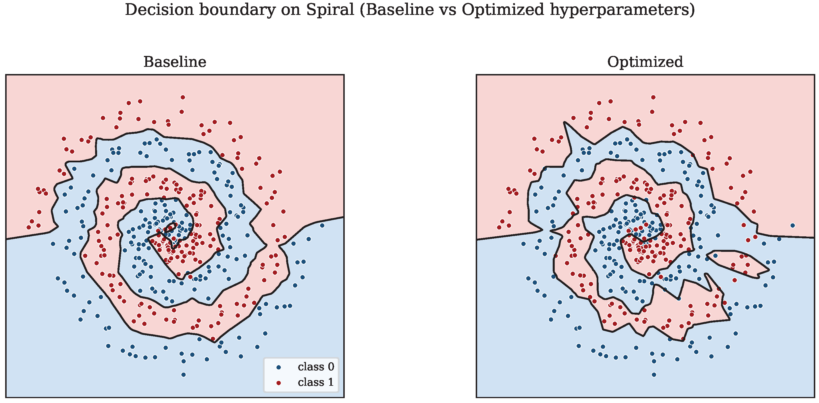
A qualitative confirmation that the weight-norm reduction does not destroy the classification structure is provided in Figure 7, which plots the decision boundary of both networks on the Spiral dataset. Both classifiers separate the two intertwined arms of the spiral correctly on most of the support of the data; the L-BFGS-B-tuned classifier produces a slightly smoother boundary, consistent with a smaller weight norm and the standard intuition that stronger L2 regularization yields more regular decision frontiers [2].

Figure 7. Decision boundary of the baseline (left) and L-BFGS-B-tuned (right) network on Spiral; the contour $\widehat{y}=0.5$ separates the classes.

5.7. Sensitivity to the Compactness Weight $\gamma$

The argument above relies on $\gamma$ being small enough that classification, rather than compactness, dominates the upper-level objective (9). To make this dependence explicit and quantitative, we sweep $\gamma$ over more than two decades and, for each value, locate the global minimizer of $f(\lambda ,\alpha )$ on the same $18\times 18$ logarithmic grid over $\mathcal{B}$ used in Figure 6 (Spiral, $(h_1,h_2)=(48,24)$, $N_{\mathrm{pre}}=200$). Reading the minimizer off the grid isolates the effect of $\gamma$ on the objective landscape itself, independently of the local behavior of the finite-difference L-BFGS-B iteration. Table 2 reports the minimizing pair $({\lambda }^{★},{\alpha }^{★})$ together with the binary cross-entropy and the classification accuracy attained there.

Table 2. Sensitivity of the upper-level objective to the compactness weight $\gamma$ (Spiral, architecture $(48,24)$, $N_{\mathrm{pre}}=200$). For each $\gamma$, the row reports the global minimizer $({\lambda }^{★},{\alpha }^{★})$ of f over the $18\times 18$ logarithmic grid of Figure 6, with the BCE and classification accuracy attained at that minimizer. Only $\gamma =2\times {10}^{-3}$ keeps the minimizer inside the useful small-$\lambda$ basin.

$\mathit{\gamma }$	${\mathit{\lambda }}^{\mathbf{★}}$	${\mathit{\alpha }}^{\mathbf{★}}$	$\mathbf{BCE}$	Acc.	Regime
$2\times {10}^{-3}$	$1.72\times {10}^{-3}$	$5.0\times {10}^{-2}$	$0.308$	$95.2\%$	small-$\lambda$ basin
$2\times {10}^{-2}$	$5.08\times {10}^{-2}$	$5.0\times {10}^{-2}$	$0.693$	$50.0\%$	near-zero-weight ridge
$1\times {10}^{-1}$	$5.08\times {10}^{-2}$	$5.0\times {10}^{-2}$	$0.693$	$50.0\%$	near-zero-weight ridge
$2\times {10}^{-1}$	$1.00\times {10}^{-1}$	$5.0\times {10}^{-2}$	$0.693$	$50.0\%$	ridge (${\lambda }^{★}={\lambda }_{max}$)
$5\times {10}^{-1}$	$1.00\times {10}^{-1}$	$5.0\times {10}^{-2}$	$0.693$	$50.0\%$	ridge (${\lambda }^{★}={\lambda }_{max}$)

The trend is sharp. At $\gamma =2\times {10}^{-3}$, the global minimizer remains inside the small-$\lambda$ basin (${\lambda }^{★}\approx 1.7\times {10}^{-3}$) and yields a usable classifier ($95.2\%$ accuracy, $\mathrm{BCE}=0.308$). For every larger value the minimizer migrates onto the near-zero weight ridge: ${\lambda }^{★}$ climbs to, and then saturates at, ${\lambda }_{max}={10}^{-1}$; the accuracy collapses to chance ($50.0\%$); and the BCE locks at $-log0.5\approx 0.693$, exactly the chance reference identified in the surface analysis of Figure 6. Beyond this threshold, the compactness term dominates and the formulation degenerates into the trivial near-zero weight solution. The chosen value $\gamma =2\times {10}^{-3}$ is thus the stable operating point used throughout Table 1: it is the largest tested weight that still leaves the objective minimizer in the operationally meaningful region.

5.8. Discussion

The norm reductions in Table 1 are larger than $25\%$ on four out of five datasets, beyond the few-percent variability observed for fixed hyperparameters, and the same pattern is visible in Figure 4. The largest accuracy degradation (4 percentage points) occurs on Spiral, the hardest dataset; the optimized network reaches $94\%$ with a much smaller norm, and a longer inner training horizon could reduce this gap at greater computational cost. Finally, the bounds in (10c) and (10d) are essential: as quantified in the $\gamma$-sensitivity analysis of Section 5.7 (Table 2), increasing $\gamma$ beyond $2\times {10}^{-3}$ drives the upper-level minimizer to ${\lambda }^{★}={\lambda }_{max}$ and collapses accuracy to chance, confirming that a small $\gamma$ together with a finite upper regularization bound is necessary for a usable formulation [3,4].

6. Conclusions

We presented a nonlinear programming framework with integer-parameterized architectures for compact-weight training of a two-hidden-layer feed-forward classifier. The upper level minimizes a weight norm-augmented BCE over a compact box of $(\lambda ,\alpha )$ values, the lower level returns the deterministic Adam output $W_N(\lambda ,\alpha )$, and finite architectural sets can be handled by outer enumeration. Theorem 1 proves lower-level coercivity and attainment under full-parameter L2 regularization; Theorem 2 gives upper-level attainment under lower semi-continuity; and Proposition 1 states conditional KKT accumulation for projected L-BFGS-B with finite differences, with the implementation gap made explicit in Remark 6. On five synthetic datasets and the fixed architecture $(48,24)$, the method reduces the Frobenius weight norm by 6.4–43.7%, with no accuracy loss on two datasets and at most a 4 percentage-point loss on Spiral.

The surface analysis in Figure 6 shows why the upper bound ${\lambda }_{max}$ is structurally important: it limits the influence of the trivial near-zero weight ridge and keeps the search inside a compact, operationally meaningful region. Future work should activate the integer level on larger architectural sets, replace finite differences with analytic or implicit gradients of the Adam recursion, and extend the formulation to multi-class classification through softmax and categorical cross-entropy.

References

- Goodfellow, I.; Bengio, Y.; Courville, A. Deep Learning; MIT Press: Cambridge, MA, USA, 2016. [Google Scholar]
- Bishop, C.M. Pattern Recognition and Machine Learning; Springer: New York, NY, USA, 2006. [Google Scholar]
- Snoek, J.; Larochelle, H.; Adams, R.P. Practical Bayesian optimization of machine learning algorithms. Adv. Neural Inf. Process. Syst. 2012, 25, 2951–2959. [Google Scholar]
- Bergstra, J.; Bengio, Y. Random search for hyper-parameter optimization. J. Mach. Learn. Res. 2012, 13, 281–305. [Google Scholar]
- Byrd, R.H.; Lu, P.; Nocedal, J.; Zhu, C. A limited memory algorithm for bound constrained optimization. SIAM J. Sci. Comput. 1995, 16, 1190–1208. [Google Scholar] [CrossRef] [Scilit]
- Zhu, C.; Byrd, R.H.; Lu, P.; Nocedal, J. Algorithm 778: L-BFGS-B: Fortran subroutines for large-scale bound-constrained optimization. ACM Trans. Math. Softw. 1997, 23, 550–560. [Google Scholar]
- Nocedal, J.; Wright, S.J. Numerical Optimization, 2nd ed.; Springer: New York, NY, USA, 2006. [Google Scholar]
- Kingma, D.P.; Ba, J. Adam: A method for stochastic optimization. In Proceedings of the 3rd International Conference on Learning Representations (ICLR), San Diego, CA, USA, 7–9 May 2015. [Google Scholar]
- Ortega-Chávez, K.L.; Fernández-Fernández, Y. Entrenamiento Eficiente en Memoria de Redes Neuronales Mediante Programación No Lineal, v1.0.0; Zenodo: Geneva, Switzerland, 2026. [CrossRef]
- Bertsekas, D.P. Nonlinear Programming, 2nd ed.; Athena Scientific: Belmont, MA, USA, 1999. [Google Scholar]
- Virtanen, P.; Gommers, R.; Oliphant, T.E.; Haberland, M.; Reddy, T.; Cournapeau, D.; Burovski, E.; Peterson, P.; Weckesser, W.; Bright, J.; et al. SciPy 1.0: Fundamental algorithms for scientific computing in Python. Nat. Methods 2020, 17, 261–272. [Google Scholar] [CrossRef] [Scilit] [PubMed]
Disclaimer/Publisher’s Note: The statements, opinions and data contained in all publications are solely those of the individual author(s) and contributor(s) and not of MDPI and/or the editor(s). MDPI and/or the editor(s) disclaim responsibility for any injury to people or property resulting from any ideas, methods, instructions or products referred to in the content. |
© 2026 by the authors. Licensee MDPI, Basel, Switzerland. This article is an open access article distributed under the terms and conditions of the Creative Commons Attribution (CC BY) license.