


Abstract
This work examines the implementation and evaluation of shortest-path algorithm in a Geographic Information System environment integrating QGIS with a PostgreSQL/PostGIS spatial database. Spatial edge and junction layers stored in the PostgreSQL/PostGIS define a directed weighted network in which edge costs are derived from spatial distance and modified through a gradient-based cost function. The routing algorithm is implemented in Python using the PyQGIS library and a binary heap priority queue. Network data are loaded from the geodatabase and processed in memory to compute the optimal route between selected nodes. The resulting path is reconstructed as a dissolved polyline feature stored in the geodatabase and visualized within the GIS environment. The study also includes a theoretical comparison of several classical shortest-path algorithms—Dijkstra, , Bellman–Ford, and Floyd–Warshall—with respect to their applicability to sparse spatial graphs typical of transportation networks. The analysis confirms the suitability of Dijkstra’s algorithm for such networks and demonstrates that routing outcomes depend directly on the definition of the edge cost function. The proposed workflow relies exclusively on open-source GISs and database technologies.
1. Introduction
Computing the shortest path between two locations in a spatial network is a core operation in Geographic Information Systems (GISs) [1] and supports applications such as transportation planning, navigation services, logistics optimization, and emergency response coordination [2]. Spatial networks are commonly represented as weighted directed graphs , where vertices (V) correspond to network junctions and edges (E) represent spatial connections such as road segments. Each edge is associated with a traversal cost that may represent geometric distance, travel time, or a composite impedance value derived from multiple attributes.
Shortest-path computation occupies an important place in graph algorithms and network optimization. Dijkstra’s algorithm remains one of the most widely used methods for computing shortest paths from a single source node in graphs with non-negative edge weights [1]. When implemented with a priority queue, the algorithm achieves a time complexity of , which makes it suitable for sparse graphs characteristic of transportation networks [2]. Other algorithms address different computational requirements. The algorithm extends Dijkstra’s framework by incorporating a heuristic estimate that guides the search toward the destination. Bellman–Ford supports graphs containing negative edge weights, while Floyd–Warshall computes shortest paths between all pairs of vertices.
Shortest-path algorithms are widely integrated into modern GIS software. Database-oriented solutions such as pgRouting implement routing within PostgreSQL/PostGIS infrastructures [3]. High-performance routing engines including OSRM and Valhalla are designed for large-scale navigation services and web-based routing applications [4,5]. Commercial GIS platforms such as ArcGIS Network Analyst provide advanced routing functionality but typically abstract the underlying algorithms from the user. Implementations that combine algorithm execution, spatial data management, and visualization within PostgreSQL/PostGIS spatial database environments are less frequently described in the literature [6]. Recent studies have examined the performance characteristics of shortest-path algorithms across different graph densities and structures [7], with comprehensive reviews of urban path-planning algorithms demonstrating the evolution from classical graph-based methods to modern machine learning approaches [8]. Python-based tools such as OSMnx have emerged as powerful platforms for downloading, modeling, and analyzing urban street networks from OpenStreetMap data [9], supporting geographic analysis across multiple disciplines.
The present work describes the implementation of Dijkstra’s shortest-path algorithm in an open-source GIS environment using Python and QGIS. A directed weighted graph is constructed from spatial layers stored in a PostgreSQL/PostGIS database. The routing algorithm operates on an in-memory graph representation and determines the shortest path between selected network nodes. The resulting route is reconstructed from the predecessor structure and written back to the geodatabase as a polyline feature that can be visualized and analyzed within the GIS environment.
Two additional aspects relevant to spatial routing are considered. The first concerns the computational characteristics of several classical shortest-path algorithms—Dijkstra, , Bellman–Ford, and Floyd–Warshall—when applied to sparse graph structures typical of GIS datasets. Previous empirical studies have confirmed theoretical complexity orderings, with priority-queue implementations of Dijkstra and providing asymptotically superior performance for sparse graphs. The second concerns the definition of the edge cost model and its influence on route selection [10]. Real-world routing systems often update edge costs dynamically according to traffic conditions and network state [11]. A spatially varying cost modifier is introduced in order to examine how changes in edge weights influence the structure of the computed routes.
2. Materials and Methods
2.1. System Architecture and Software Environment
The routing system was implemented in the open-source QGIS environment using Python 3.11.11 and the PyQGIS 3.44. Spatial data are stored in an open spatial database implemented in PostgreSQL 14 with the PostGIS 3.x extension. The routing script operates as a standalone Python module executed within the QGIS Python environment based on Python 3.9. The system reads spatial network data directly from the PostgreSQL/PostGIS database through a standard database connection.
The system reads spatial network data directly from the geodatabase through a standard database connection and performs shortest-path computation in Python memory. The resulting route geometry is written back to the database as a polyline layer and visualized within QGIS.
This architecture separates spatial data storage from algorithm execution: spatial layers are managed within the PostgreSQL/PostGIS database, while graph processing and path computation are performed in Python. The approach allows full control over the routing logic while preserving compatibility with standard GIS workflows and visualization tools.
2.2. Spatial Data Model and Test Network
The spatial network is represented by three spatial layers stored in the PostgreSQL/PostGIS database. The junctions layer represents network nodes. Each record contains a unique identifier (node_id) and the spatial coordinates of the node stored in the geometry field. Junctions correspond to intersections or terminal points in the spatial network.
The edge layer represents directed connections between nodes. Each edge contains the attributes from_id, to_id, cost, and edge_id, together with the polyline geometry describing the spatial segment. The directed structure of the graph is defined by the from_id → to_id relationship. Bidirectional road segments are represented as two separate edge records with opposite direction.
The route_results layer stores the routing output. Each computed route is written as a polyline feature with attributes describing the start node, end node, total cost, and the number of traversed edges.
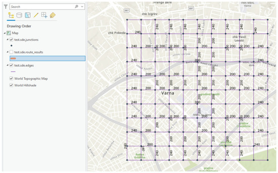
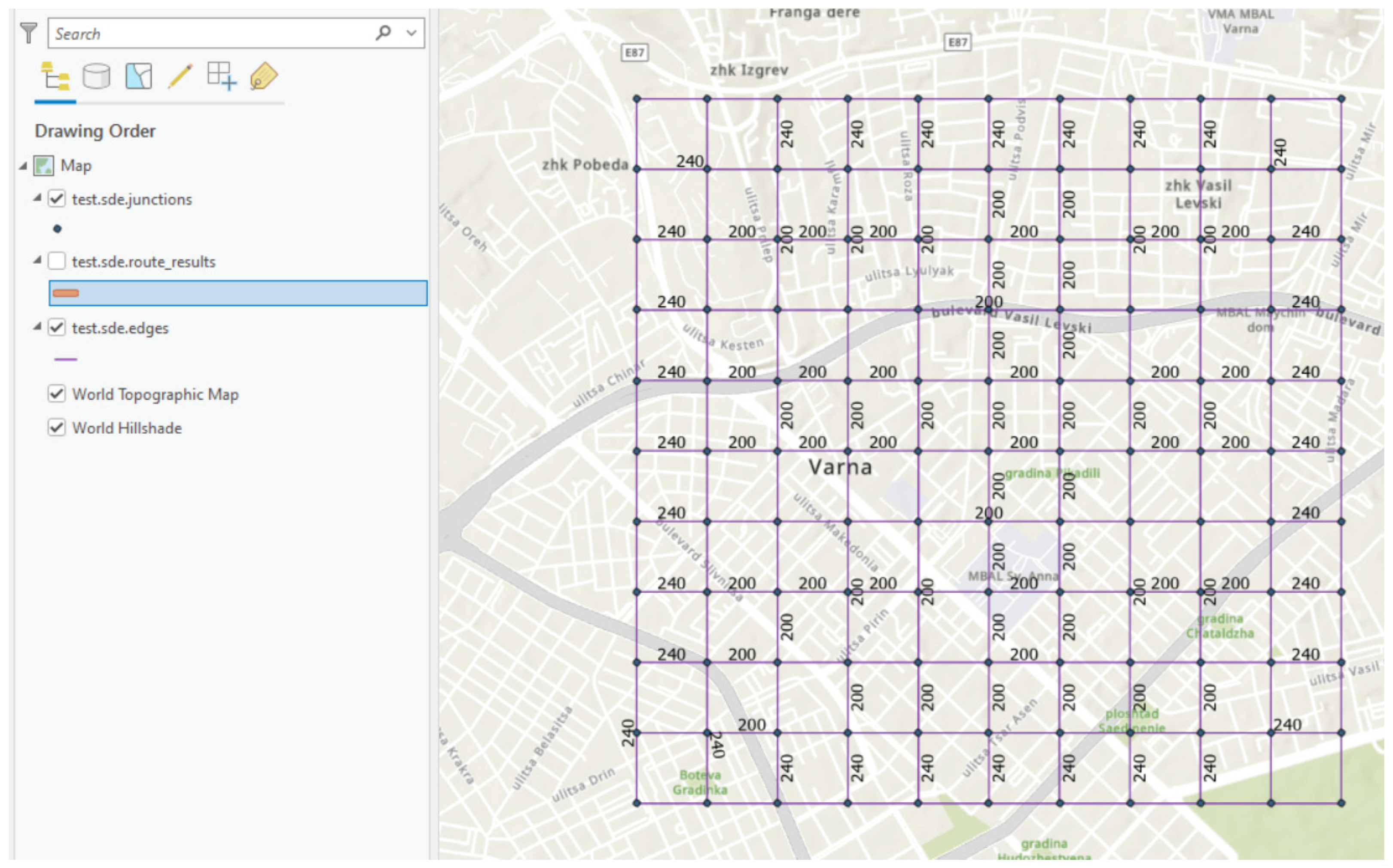
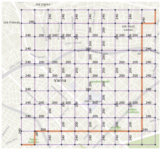
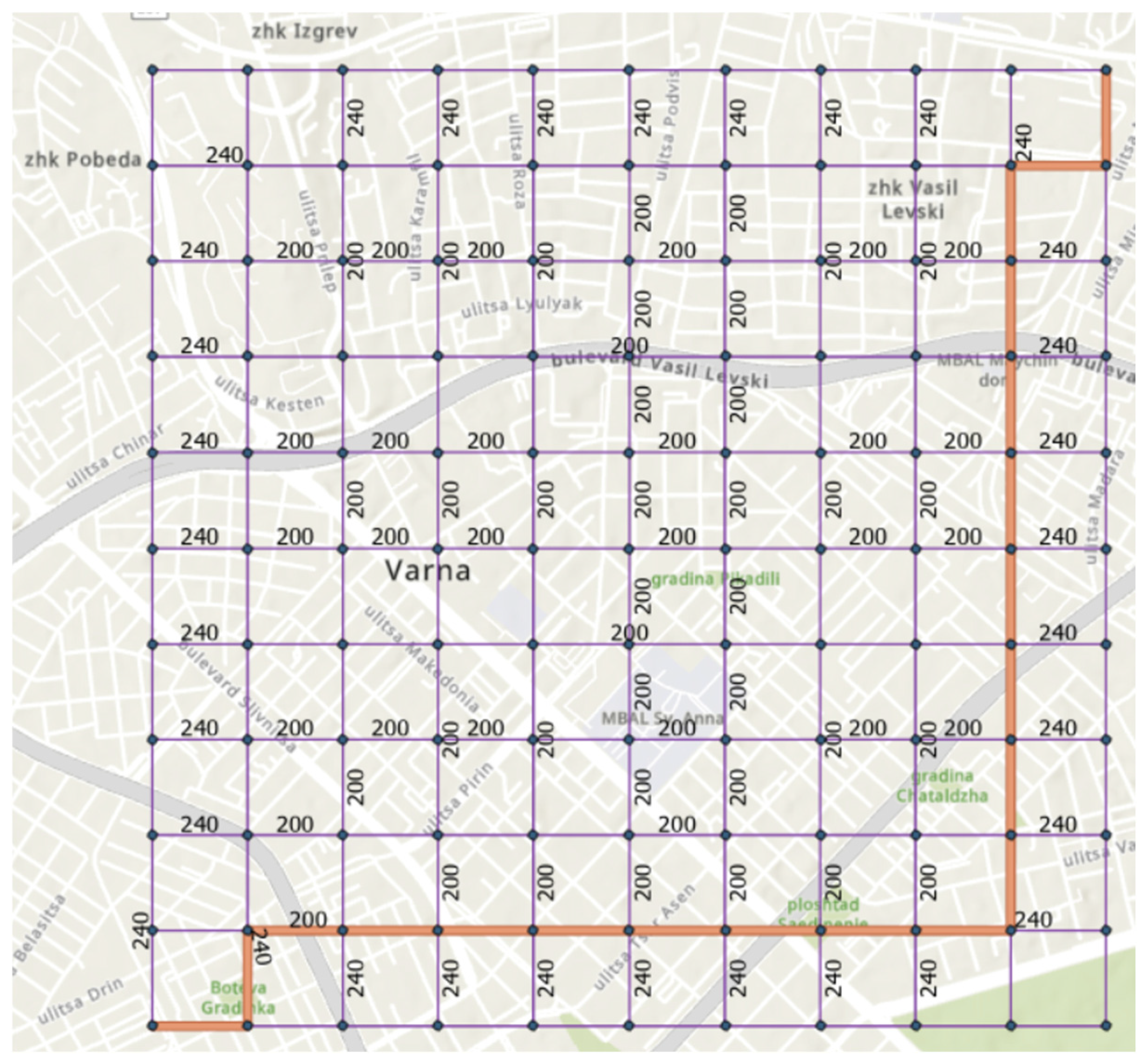
For controlled testing and algorithm verification, a synthetic orthogonal grid network was generated programmatically over a base map of Varna, Bulgaria (Figure 1). The grid structure allows deterministic verification of routing results because shortest paths under uniform edge weights follow predictable Manhattan-style trajectories.
Figure 1.
Orthogonal grid network overlaid on a base map.
The full test network contains 121 nodes arranged in an 11 × 11 grid. Directed edges connect horizontally and vertically adjacent nodes. Smaller subnetworks (3 × 3, 5 × 5, and 9 × 9) were derived from the base grid to evaluate algorithm behavior on graphs of different sizes.
2.3. Edge Cost Function
Each edge is assigned a traversal cost stored in the cost attribute. The base cost corresponds to the Euclidean length of the spatial segment.
To examine the effect of cost-model design on routing behavior, a gradient-based cost modifier was introduced. The modifier increases traversal cost for edges located near the outer boundary of the network while preserving the original graph topology.
Let denote the midpoint of edge and the geometric center of the network. A normalized peripheral distance is defined as
where is the node farthest from the center. The modified traversal cost becomes
where is a configurable penalty coefficient.
For , the routing problem reduces to the standard shortest-path problem based on Euclidean distance [12]. Increasing gradually penalizes peripheral edges and biases routing toward the central region of the network. This parameterization allows controlled analysis of how routing outcomes depend on cost–model assumptions.
2.4. Graph Construction and Algorithm Implementation
The spatial graph is loaded from the PostgreSQL/PostGIS database into memory using PyQGIS feature iteration and attribute access. For each record, the algorithm extracts the origin node, destination node, traversal cost, and edge identifier. The graph is stored as an adjacency list structure
where is the origin node, the destination node, the traversal cost, and edge_id identifies the corresponding spatial segment. Loading the graph requires time and memory. The adjacency-list representation keeps the graph structure compact while maintaining a direct reference to the original spatial segment through the stored edge identifiers. This makes it possible to reconstruct the spatial route directly from the computed sequence of edges.
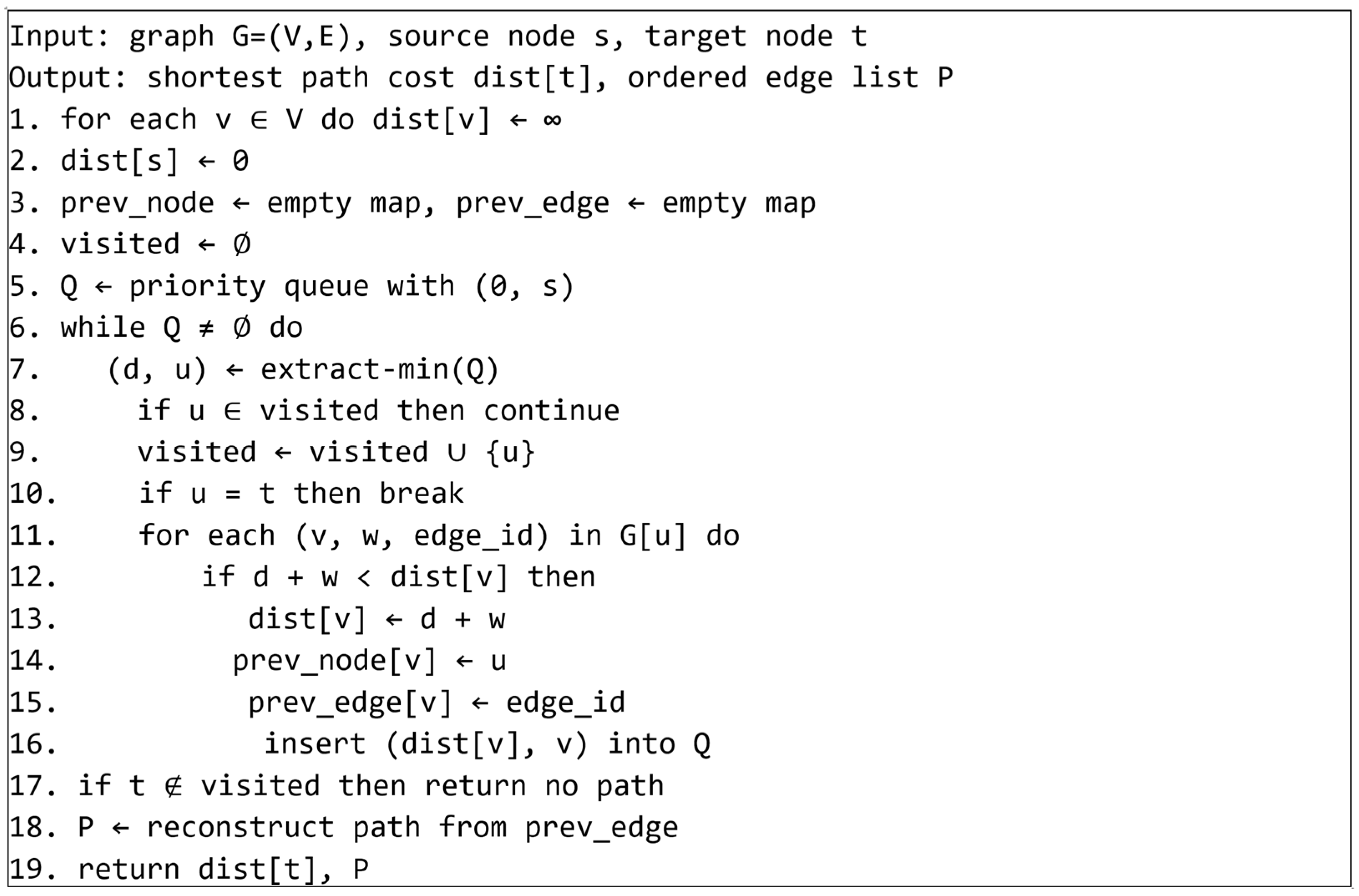
Shortest-path computation is performed using Dijkstra’s algorithm with a binary min-heap priority queue implemented through Python’s heapq module. Each queue element contains a pair (distance, node), representing the current tentative distance to a vertex.
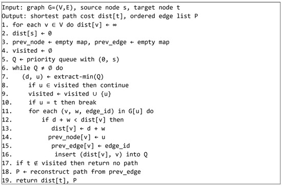
The implementation uses a visited-set strategy together with lazy deletion of outdated queue entries. Distance estimates are stored in a dictionary dist, while two predecessor dictionaries (prev_node and prev_edge) track the structure of the shortest-path tree. These dictionaries allow reconstruction of the final route as an ordered sequence of edge identifiers once the target node has been reached. The pseudocode shown in Figure 2 summarizes the main steps of the implementation.
Figure 2.
Dijkstra shortest-path algorithm using a binary heap.
The priority queue ensures that nodes are explored in non-decreasing order of distance from the source vertex. Once a vertex is extracted from the queue its shortest-path distance is final.
2.5. Route Geometry Construction and Output Generation
After the shortest path has been determined, the resulting sequence of edge identifiers is used to reconstruct the spatial geometry of the route. The corresponding network segments are selected from the spatial dataset and merged into a single polyline geometry.
The merging process is performed using the GIS dissolve operation, which combines multiple line features into a single geometry while preserving topological continuity. The resulting polyline represents the computed route between the selected start and end nodes.
The reconstructed route is then written to a dedicated output layer in the PostgreSQL/PostGIS database. Additional attributes are stored together with the geometry, including the identifiers of the start and end nodes, the total traversal cost, and the number of edges forming the route. This integration enables the computed route to be visualized directly within the GIS environment and used in subsequent spatial analysis or decision-support workflows.
3. Results
3.1. Theoretical Complexity Comparison
The shortest-path problem in spatial networks can be solved by several classical graph algorithms. Their practical applicability depends primarily on computational complexity and on the structural characteristics of the underlying graph. Metaheuristic optimization techniques, including improved discrete algorithms and hybrid approaches, are widely applied to routing problems in transportation systems with real-time constraints [12]. Multimodal transportation networks introduce additional complexity requiring robust path planning strategies [13]. Table 1 summarizes the theoretical time and space complexity of the algorithms considered in this study.
Table 1.
Complexity characteristics of selected shortest-path algorithms.
The ordering O(E + V log V) << O(V·E) << O(V3) determines the relative suitability of the algorithms for sparse spatial graphs. Road networks typically satisfy the condition , meaning that the number of edges grows approximately linearly with the number of nodes. Under these conditions Dijkstra’s algorithm and are asymptotically more efficient than Bellman–Ford and Floyd–Warshall.
The synthetic grid network used in this study contains 121 vertices and 220 directed edges. The ratio clearly places the graph in the sparse regime, where priority-queue implementations of Dijkstra or provide the most appropriate computational strategy.
Previous empirical studies have confirmed this theoretical ordering. Sapundzhi et al. [7] report execution times several orders of magnitude lower for Dijkstra compared to Floyd–Warshall on sparse directed graphs with several hundred vertices. These results are consistent with the algorithm selection adopted in the present work.
3.2. Qualitative Comparison of Algorithm Behaviour
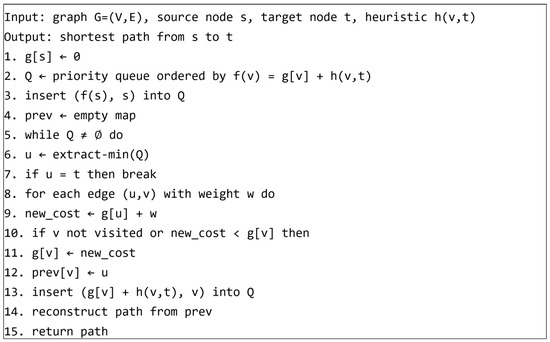
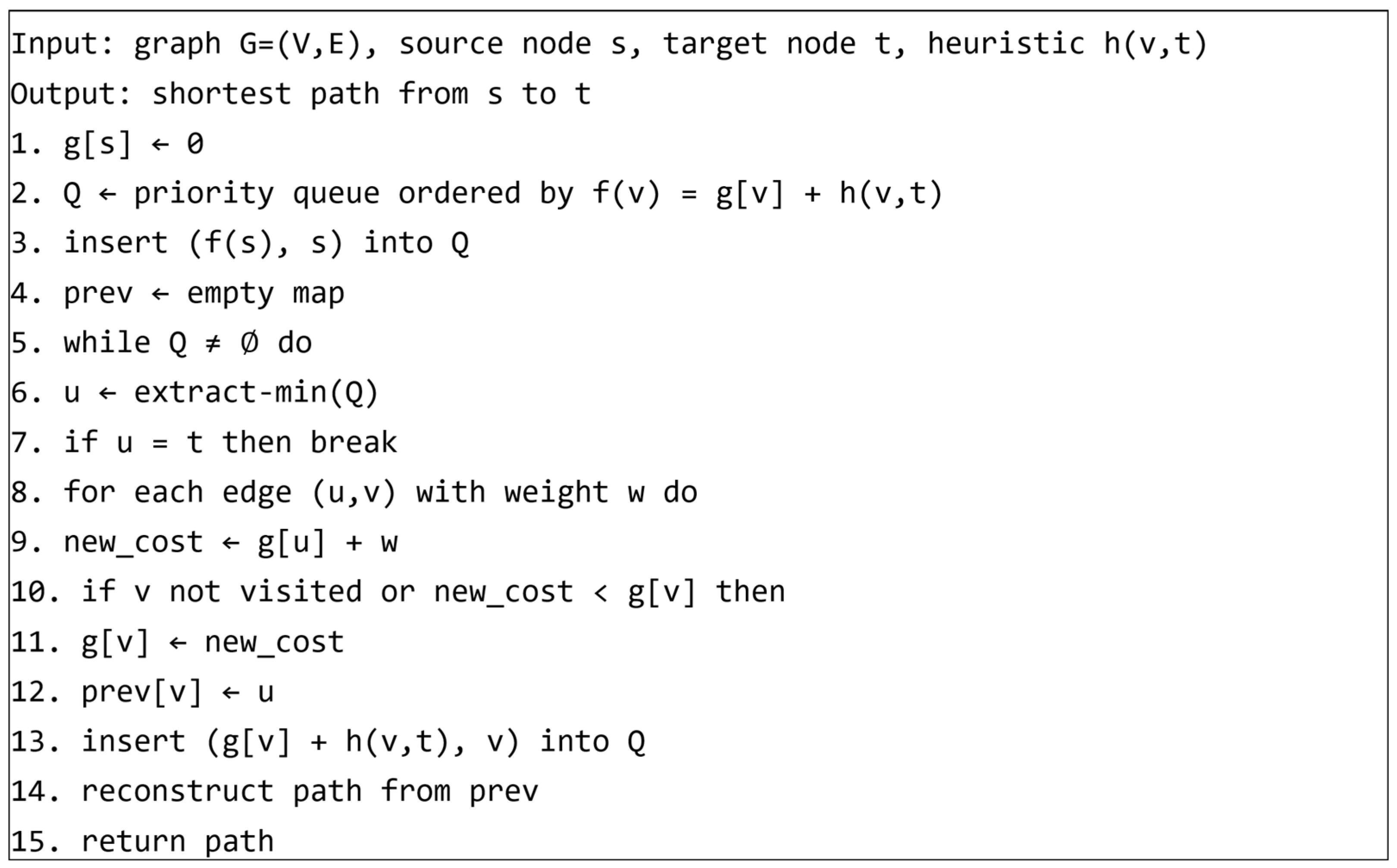
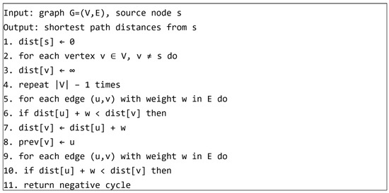
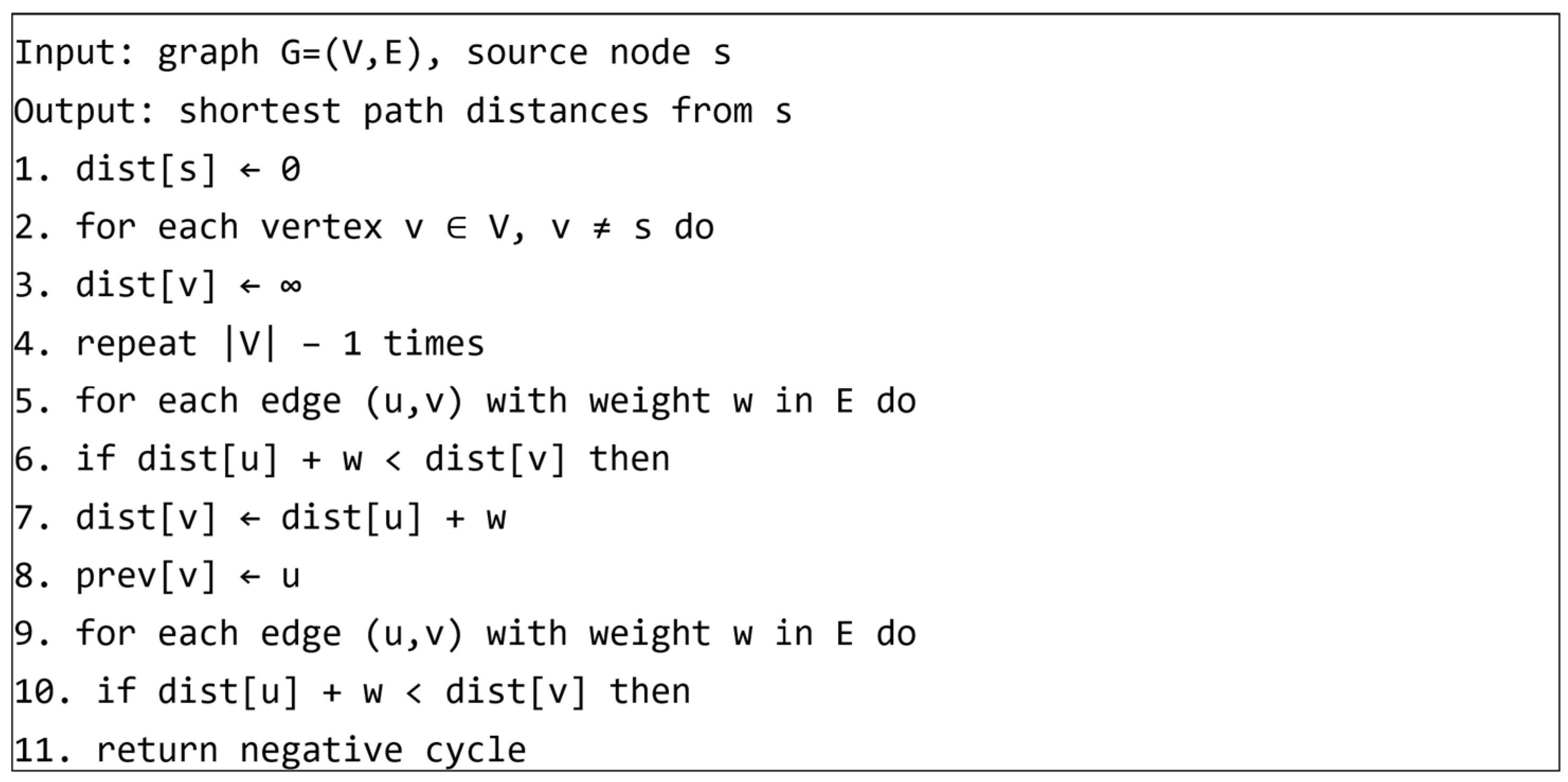
Shortest-path algorithms follow different search strategies that influence graph exploration and path evaluation during routing. The main operational steps of two representative algorithms— and Bellman–Ford—are summarized below to illustrate the differences in their search strategies. Figure 3 and Figure 4 present the pseudocode of the and Bellman–Ford algorithms, illustrating their main operational steps.
Figure 3.
Pseudocode of the search algorithm using the heuristic evaluation function.
Figure 4.
Pseudocode of the Bellman–Ford algorithm for computing shortest paths and detecting negative cycles in weighted graphs.
Dijkstra’s algorithm expands vertices in non-decreasing order of distance from the source node. Once a node is removed from the priority queue, its shortest-path distance is guaranteed to be final. This property allows early termination when the target node is reached, which is particularly advantageous for single-pair routing queries.
The algorithm modifies the priority queue ordering by introducing a heuristic function
where represents the current path cost from the source node and estimates the remaining cost to the target node t. In spatial networks the straight-line Euclidean distance between nodes provides a natural admissible heuristic. When such geometric information is available, reduces the number of explored nodes by directing the search toward the destination.
Bellman–Ford follows a different strategy based on repeated relaxation of all edges in the graph. While this approach allows the algorithm to handle negative edge weights and detect negative cycles, it requires substantially more relaxation operations than Dijkstra’s priority-queue approach when weights are non-negative.
Floyd–Warshall computes the complete matrix of shortest paths between all pairs of vertices. The algorithm is therefore suitable when a large number of routing queries must be answered on the same static graph. For single-pair routing tasks, however, the complexity makes it computationally inefficient compared to single-source algorithms.
Dijkstra’s algorithm and its heuristic variant are therefore well suited for routing in sparse spatial networks with non-negative edge weights.
3.3. Behaviour of the Implemented System
The implemented Dijkstra algorithm was tested on the synthetic grid network described in Section 2.2. The source node was fixed at node 1, while the destination node corresponded to the opposite corner of the grid (node 121).
The algorithm successfully identified the optimal route and returned the sequence of edge identifiers forming the shortest path. The deterministic structure of the grid network allows direct verification of algorithm correctness because optimal paths follow predictable Manhattan-type trajectories. The predecessor dictionaries produced during the search allowed direct reconstruction of the route without additional graph traversal.
The computed route geometry was constructed by selecting the corresponding polyline segments and merging them using the dissolve functionality available in QGIS. The resulting polyline was inserted into the route_results feature class and visualized in QGIS. Visual inspection confirmed that the route forms a continuous path between the source and destination nodes without topological inconsistencies (Figure 5).
Figure 5.
Visualization of the network and the route_results output layer—QGIS.
For the largest test network (121 nodes and 220 edges), the entire workflow—including graph loading, shortest-path computation, and route reconstruction—completed within a few milliseconds in the QGIS Python environment. These observations indicate that in-memory processing combined with a binary-heap priority queue provides sufficient performance for medium-scale spatial networks typically encountered in desktop GIS workflows.
3.4. Influence of the Gradient Cost Function on Route Selection
The implemented system includes a parametric gradient cost function described in Section 3.3. This mechanism illustrates that routing results produced by Dijkstra’s algorithm are entirely determined by the definition of the edge cost function.
On the 11 × 11 orthogonal grid, the theoretical behavior under the two weight configurations can be analyzed exactly. Under uniform weights (α = 0), all edges of equal geometric length are interchangeable; any shortest path from node (1,1) to node (11,11) traverses exactly 20 edges (10 horizontal + 10 vertical in any order) for a total Euclidean cost of 2000 m. Multiple shortest paths exist, and the tie-breaking behavior of the priority queue determines which is returned. Under gradient-modified weights (α > 0), peripheral edges located in the outer rows and columns of the grid—receive elevated cost multipliers, making paths along the boundary more expensive. As α increases, the optimal path progressively migrates inward toward the central corridor of the grid, trading a larger edge count for a lower total weighted cost. This behavior is consistent with the theoretical optimality of Dijkstra’s algorithm with respect to the defined cost function. Parameterized cost functions are widely used in transportation routing applications such as electric-vehicle route planning, where charging time, energy consumption, and station availability influence route selection [14].
This sensitivity to cost function parameterization has direct practical relevance in real-world GIS routing applications. Edge weights in transportation networks commonly incorporate composite impedance values such as road category, surface condition, gradient, congestion level, or environmental exposure index rather than pure Euclidean distance. The gradient cost experiment illustrates that careful cost function design is as critical to routing quality as algorithm selection, and that the PyQGIS implementation framework provides full flexibility to define and test alternative cost models without modifying the algorithmic core. The experiment therefore confirms that route geometry in shortest-path routing is determined not only by network topology but also by the mathematical structure of the cost function applied to the edges.
4. Discussion
4.1. Practical Implications for GIS Routing
The theoretical complexity analysis together with the observed behavior of the implemented system support the use of Dijkstra’s algorithm for single-source shortest-path computation in sparse spatial networks with non-negative edge weights, consistent with empirical findings reported in prior literature [7]. Urban mobility planning systems use optimized shortest-path algorithms within transportation network models. These methods are applied in emergency evacuation routing, multimodal transport planning, and electric vehicle infrastructure management [13,14]. As these routing services become integrated into enterprise software platforms, implementation quality and security considerations become increasingly important for reliable operation [15]. A grid equivalent to a 500 × 500 street network (V ≈ 250,000 nodes) remains within the practical performance range of Dijkstra’s algorithm.
The open-source QGIS/PyQGIS integration pattern developed in this work provides a transparent and replicable framework for embedding custom routing logic within enterprise GIS workflows. Several architectural decisions contribute to this behavior. The implementation loads the complete graph into Python memory (O(V + E) space) rather than issuing per-node SQL queries and uses lazy deletion in the priority queue instead of decrease-key operations. Edge identifiers are retained in the adjacency list, which allows geometric route reconstruction in O(path_length) time without additional database queries. These decisions ensure that the implementation is both algorithmically efficient and practically operable within the QGIS environment.
4.2. Limitations
Several limitations of the current implementation should be acknowledged. The synthetic orthogonal grid topology provides a controlled experimental environment but does not fully represent real-world street network characteristics, which include irregular node degrees, non-uniform edge length distributions, and complex intersection geometries. The directed graph model correctly handles one-way road segments, but turn restrictions—which model prohibited turning movements at intersections—are not currently supported; in practice, turn restrictions require augmenting the graph with edge-to-edge transition nodes, adding complexity to both the data model and the algorithm.
The comparison with assumes availability of Euclidean node coordinates for heuristic computation. In geodatabases where junction coordinates are not stored as explicit attributes, an additional spatial query would be required to populate the coordinate dictionary, adding loading overhead. Furthermore, the Euclidean heuristic is admissible but not necessarily tight for non-grid networks with winding roads, potentially reducing ’s advantage over Dijkstra in irregular network topologies.
Memory usage was not systematically measured in the present study. The O(V2) space requirement of Floyd–Warshall makes it impractical for networks exceeding approximately 10,000 nodes on typical workstation hardware. The current graph loading approach reads the full edge set into memory; for very large networks (E > 106), a tile-based or streaming approach would be necessary.
4.3. Comparison with pgRouting
The pgRouting extension for PostgreSQL provides functionally equivalent routing capabilities directly within the database engine, with Dijkstra implemented as the pgr_dijkstra() function. The primary advantage of the PyQGIS-based approach presented here is the tight integration with the QGIS cartographic environment: route results are immediately available as symbolized feature layers without requiring an additional data export or ETL step. The pgRouting approach, conversely, enables routing queries to be issued via SQL from any client application, is more suitable for high-throughput server-side routing, and supports topology validation through the pgr_createTopology() preprocessing function. For use cases requiring interactive spatial visualization and GIS analyst workflows within QGIS, the PyQGIS implementation is preferable; for web service backends or database-centric architectures, pgRouting is the more appropriate choice.
5. Conclusions
Shortest-path routing forms a fundamental component of many GIS-based transportation and infrastructure analyses. The implemented system integrates graph–algorithm computation with the QGIS environment and PostgreSQL/PostGIS. Spatial edge features are transformed into an in-memory directed weighted graph processed through a Python/PyQGIS implementation of Dijkstra’s algorithm, after which the resulting path is reconstructed and stored as a polyline feature in the geodatabase. This architecture enables direct interaction between algorithmic routing procedures and standard GIS visualization workflows.
Evaluation on a synthetic grid network confirms that priority-queue implementations of Dijkstra’s algorithm perform efficiently on sparse spatial graphs typical of road networks. The gradient cost experiment further illustrates how routing outcomes depend directly on the definition of edge weights. Changes in the cost model alter the geometry of the computed route without modifying the underlying network topology. In practical GIS routing systems, impedance values often incorporate multiple factors such as road category, slope, congestion level, or environmental exposure.
The QGIS/PyQGIS-based framework enables reproducible experimentation with routing models in an open and freely accessible GIS environment while preserving compatibility with existing geodatabase workflows. Future work will focus on validation with real street network datasets, extension of the data model to support turn restrictions and time-dependent edge weights, and comparative evaluation of additional routing strategies for large-scale spatial networks.
Author Contributions
V.S., A.I., F.S. and S.G. contributed equally to this work. All authors have read and agreed to the published version of the manuscript.
Funding
This study was financed by the European Union—NextGenerationEU, through the National Recovery and Resilience Plan of the Republic of Bulgaria, project No. BG-RRP-2.013-0001.
Institutional Review Board Statement
Not applicable.
Informed Consent Statement
Not applicable.
Data Availability Statement
The source code and synthetic test data are available from the corresponding author upon request.
Conflicts of Interest
The authors declare no conflicts of interest.
Abbreviations
The following abbreviations are used in this manuscript:
| GIS | Geographic Information System |
| SDE | Spatial Database Engine (Esri Enterprise Geodatabase) |
| ArcPy | ArcGIS Python scripting library |
| PostGIS | Spatial extension for PostgreSQL |
References
- Abed, S.S.; Noaman, S.F. Comparative Analysis of Shortest Path Algorithms. South Asian Res. J. Eng. Technol. 2025, 7, 131–143. [Google Scholar] [CrossRef] [Scilit]
- Nithya, S.; R, P. Traffic Congestion Analysis and Route Optimization in an Urban Road Network Using Geographic Information System (GIS). Int. J. Res. Appl. Sci. Eng. Technol. 2026, 14, 1691–1695. [Google Scholar] [CrossRef] [Scilit]
- Sirisumrannukul, S.; Prakobkaew, P.; Piamvilai, N. Optimal Planning for Public Charging Infrastructure by Behaviour-Based Electric Vehicle Charging Demand Simulations and Geographic Information System. IET Smart Grid 2025, 9, e70050. [Google Scholar] [CrossRef] [Scilit]
- Djebnoune, B.; Guendouz, B. Analysis of Urban Transportation Network in Algerian Border Cities Using Geographic Information System (GIS): Case Study of Tébessa City—Far Northeast. Geomat. Landmanag. Landsc. 2025, 1, 233–244. [Google Scholar] [CrossRef] [Scilit]
- Selvasofia, S.D.A.; SivaSankari, B.; Dinesh, R.; Muthukumaran, N. GINSER: Geographic Information System Based Optimal Route Recommendation via Optimized Faster R-CNN. Int. J. Comput. Intell. Syst. 2025, 18, 75. [Google Scholar] [CrossRef] [Scilit]
- Cooper, C.H.V.; Chiaradia, A. sDNA: 3-D Spatial Network Analysis for GIS, CAD, Command Line & Python. SoftwareX 2020, 12, 100525. [Google Scholar] [CrossRef] [Scilit]
- Sapundzhi, F.; Danev, K.; Ivanova, A.; Popstoilov, M.; Georgiev, S. A Performance Comparison of Shortest Path Algorithms in Directed Graphs. Eng. Proc. 2025, 100, 31. [Google Scholar] [CrossRef] [Scilit]
- Tian, Z.; Yao, H.; Shao, Y. A Review of Urban Path Planning Algorithms in Intelligent Transportation Systems. Algorithms 2025, 18, 676. [Google Scholar] [CrossRef] [Scilit]
- Boeing, G. Modeling and Analyzing Urban Networks and Amenities with OSMnx. Geogr. Anal. 2025, 57, 567–577. [Google Scholar] [CrossRef] [Scilit]
- Grujić, Ž.; Grujić, B. Optimal Routing in Urban Road Networks: A Graph-Based Approach Using Dijkstra’s Algorithm. Appl. Sci. 2025, 15, 4162. [Google Scholar] [CrossRef] [Scilit]
- Benmessaoud, Y.; Cherrat, L.; Ezziyyani, M. Real-Time Self-Adaptive Traffic Management System for Optimal Vehicular Navigation in Modern Cities. Computers 2023, 12, 80. [Google Scholar] [CrossRef] [Scilit]
- Wang, R.; Zhou, M.; Wang, J.; Gao, K. An Improved Discrete Jaya Algorithm for Shortest Path Problems in Transportation-Related Processes. Processes 2023, 11, 2447. [Google Scholar] [CrossRef] [Scilit]
- Guo, J.; Liu, T.; Song, G.; Guo, B. Solving the Robust Shortest Path Problem with Multimodal Transportation. Mathematics 2024, 12, 2978. [Google Scholar] [CrossRef] [Scilit]
- Tan, A.; Wang, C.; Wan, Y.; Dong, C. Electric Vehicle Charging Route Planning for Shortest Travel Time Based on Improved Ant Colony Optimization. Sensors 2024, 25, 176. [Google Scholar] [CrossRef] [Scilit] [PubMed]
- Muhenga, R.; Sapundzhi, F.; Popstoilov, M.; Georgiev, S.; Todorov, V. Comprehensive Analysis of Cryptographic Algorithms: Implementation and Security Insights. Eng. Proc. 2025, 104, 43. [Google Scholar] [CrossRef] [Scilit]

Disclaimer/Publisher’s Note: The statements, opinions and data contained in all publications are solely those of the individual author(s) and contributor(s) and not of MDPI and/or the editor(s). MDPI and/or the editor(s) disclaim responsibility for any injury to people or property resulting from any ideas, methods, instructions or products referred to in the content. |
© 2026 by the authors. Licensee MDPI, Basel, Switzerland. This article is an open access article distributed under the terms and conditions of the Creative Commons Attribution (CC BY) license.