Quantitative Evaluation of Museum Exhibition Layouts Using Visitor Flow Analysis ^†

Abstract

Exhibition layouts in museums strongly influence visitors’ learning and viewing experiences, yet their evaluation often relies on curators’ subjective judgments. This study aims to provide objective behavioral data through visitor flow analysis to support evidence-based exhibition design. Single-board computers installed in the museum exhibition rooms serve as sensors to detect humans in captured images using machine learning. Detected positions are projected onto a floor map using a homography transformation to reconstruct visitors’ spatiotemporal behavior. The proposed system enables server-side real-time analysis and visualization, allowing curators to quickly and objectively understand visitor movement patterns.

1. Introduction

Exhibition layouts in museums and art galleries significantly influence visitor experiences and the appeal of exhibits. Curators design layouts while considering the background of each exhibit and its relationship with other exhibits; however, evaluating these layouts in practice relies on qualitative methods such as visitor questionnaires and observational records. For this reason, new methods are required to enable the quantitative evaluation of the appropriateness of exhibition layouts.

In recent years, analysis of visitor behavior has attracted attention as a method that contributes to understanding the quality of exhibition experiences, improving layouts, and enhancing learning effects. Visitor flow analysis is important for supporting evidence-based layout design, as it enables understanding of behavioral characteristics, such as which exhibits visitors are interested in, which routes they follow, and where they tend to stay.

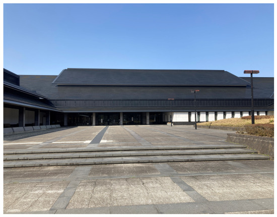
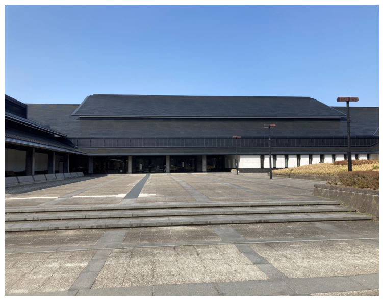
In this study, in cooperation with museum curators, visitor data are collected using sensors installed within the museum, and visitor flow analysis is conducted to apply the results to a quantitative evaluation of exhibition layouts. Figure 1 shows the target museum used in this study, the Fukushima Museum.

Figure 1. Fukushima Museum.

This study consists of the following steps. First, visitor data are acquired using sensors, and human detection is performed using machine learning. Next, detection results are projected onto a floor map using a homography transformation to estimate position information. Then, heatmaps are generated based on the estimated positions to visualize staying tendencies and movement patterns. Finally, these results are used to analyze exhibition layouts for evaluation and improvement.

This paper is structured as follows. Section 2 describes related work on visitor behavior analysis in museums and clarifies the positioning of this study. Section 3 presents the configuration of the sensor system installed in the museum, an overview of the acquired data, and explains the methods for human detection and visitor position estimation using homography transformation. Section 4 presents visualization methods for visitor flow using heatmap generation, along with analysis results from real data and their discussion. Finally, Section 5 summarizes this study and discusses future issues.

2. Related Work

Previous studies have emphasized the importance of measuring and analyzing visitor behavior to evaluate exhibition layouts and improve museum management. Traditional museum studies mainly relied on qualitative methods such as questionnaires and observational records; however, these methods are subject to bias and limited sample sizes, making comprehensive spatial analysis difficult [1].

Quantitative approaches based on behavioral tracking have therefore attracted increasing attention. Yalowitz and Bronnenkant [1] demonstrated the effectiveness of timing and tracking methods for understanding visitor stay time and movement patterns. Zancanaro et al. [2] analyzed museum visitors’ behavior patterns from a user modeling perspective and showed that behavioral regularities can be extracted to better understand visitor engagement. Strohmaier et al. [3] visualized spatial–temporal visitor flows to support curatorial decision-making. Similarly, Shapiro et al. [4] proposed the concept of interaction geography to analyze spatial interaction patterns in museum environments. These studies highlight the importance of visualizing visitor behavior for spatial evaluation.

Large-scale sensing technologies have also been applied in real museum environments. Yoshimura et al. [5] utilized Bluetooth data to analyze visitor mobility at the Louvre Museum, while Muramatsu et al. [6] employed BLE beacons and wearable devices for indoor behavior estimation. Umezu and Koizumi [7] and Umezu et al. [8] explored visitor counting and behavior analysis using LiDAR sensors, demonstrating the feasibility of non-visual sensing approaches. Saito et al. [9] investigated GPS-based data acquisition in open-air museums. Serasidis et al. [10] proposed a low-cost IoT platform for anonymous real-time visitor flow tracking. These studies illustrate the diversity of sensing modalities used in visitor behavior analysis.

Camera-based and deep-learning approaches have further advanced behavioral analysis. Ferrato et al. [11] applied deep learning to collect visitor behavior data, and Breitner and Bandung [12] performed detection and tracking under low-light surveillance conditions. Centorrino et al. [13] modeled visitor flows to improve congestion management. These works demonstrate the effectiveness of computational methods for analyzing crowd behavior and optimizing museum operations.

In addition to flow measurement, several studies have focused on knowledge experience and exhibit evaluation. Takahashi et al. [14] proposed an approach for visualizing visitor interest distribution using single-board computers to sense spatial positions of visitors. Yanada et al. [15], Tamahashi et al. [16], and Hoshino and Yoshioka [17] discussed design methodologies for knowledge creation and experiential systems in hybrid or digital museum environments. Philippopoulos et al. [18] presented a holistic approach to enhancing museum performance. Primadani et al. [19] investigated visitor responses to technology-based interactive displays. Nishidate et al. [20,21] addressed technical challenges in detecting subtle temporal changes in static environments, such as museums and art galleries, from camera-captured images. These studies suggest that behavioral data and visualization technologies contribute not only to flow analysis but also to experience design and educational effectiveness.

Overall, prior research demonstrates the effectiveness of acquiring and visualizing visitor behavior using various sensing technologies and analytical frameworks. However, few studies have integrated low-cost camera sensing, privacy-preserving position reconstruction based solely on bounding-box data, homography-based spatial mapping, and multi-scale heatmap visualization into a unified framework specifically designed for quantitative evaluation of exhibition layouts. This study addresses this gap by proposing an integrated system that combines these components for practical and scalable museum deployment.

3. Materials and Methods

3.1. Sensor Placement

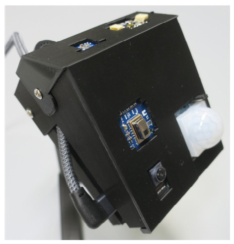
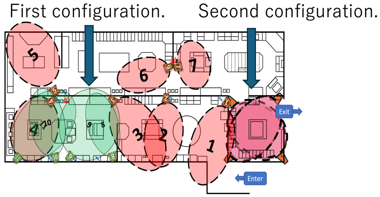
In this study, 15 Raspberry Pis (Raspberry Pi Ltd., Cambridge, UK) (see Figure 2) were installed as sensors throughout the museum’s exhibition space. Each sensor was mounted near the ceiling to provide a wide overview of the exhibition space while minimizing visitor occlusion. The fields of view of adjacent sensors partially overlap, reducing blind spots and improving detection robustness.

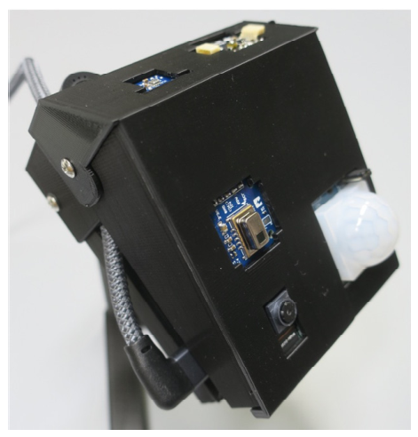
Figure 2. Raspberry Pi sensor installed in the museum.

Although all sensors were deployed within the same exhibition space, two distinct exhibition areas were used for different stages of analysis.

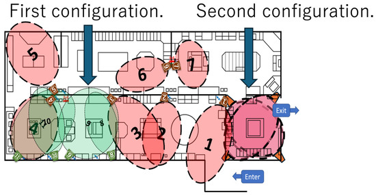
The first configuration, referred to as the bottom-left configuration, consists of Sensors 8–11, which are in the lower-left section of the exhibition space (see Figure 3). This area contains a distinct group of exhibits, separate from other sections of the space. These sensors were used for the heatmap-based spatial analysis described in Section 3.5. Data from this configuration were collected from August to October 2025, enabling long-term analysis of spatial stay tendencies within that exhibition area.

Figure 3. Floor map of the entire exhibition space and configurations of installed sensors.

The second configuration, referred to as the square-layout configuration, consists of four sensors installed in the lower-right section of the same exhibition space. The sensors in this area were added later in this research project and arranged in an approximately square configuration, allowing placement at the four corners. This geometric arrangement provides stable multi-view coverage and is particularly suitable for validating short-term trajectory estimation. The movement pattern visualization described in Section 3.6 is based on data collected from this configuration in December 2025.

The difference in sensor groups reflects the development sequence of the visualization methods: the heatmap analysis was implemented and validated using the bottom-left configuration, whereas the trail-based movement visualization was later implemented and tested using the square-layout configuration, which offers a geometrically favorable setup for trajectory verification.

Figure 3 illustrates the spatial arrangement of the installed sensors and highlights the two experimental configurations used in this study. Because the two configurations monitor different exhibition areas with distinct themes, the results are analyzed separately rather than directly compared.

3.2. Sensor System and Acquired Data

The sensors used in this study acquire data at one-minute intervals. The acquired data include illuminance, temperature, humidity, atmospheric pressure, thermography, sound volume, camera data, and Bluetooth data. These data are transmitted to a server and stored in JSON format. In this study, the stored data are used for analysis.

3.3. Human Detection and Acquisition of Coordinate Information

Human detection is performed on camera images using YOLO, a real-time object detection algorithm that encloses detected objects in bounding boxes. Each bounding box is represented by the four vertices in the image coordinate system, $\left(x_1,y_1\right),\left(x_2,y_2\right),\left(x_3,y_3\right), \mathrm{and} \left(x_4,y_4\right)$. For privacy protection, the original camera images are not transmitted to the server; only the bounding-box vertex coordinates obtained as detection results are transmitted. In this study, in order to estimate the actual position of a person on the floor plane, the two points corresponding to the bottom edge of the bounding box, $\left(x_3,y_3\right) \mathrm{a}\mathrm{n}\mathrm{d} \left(x_4,y_4\right)$, are used, and their midpoint (i.e., $\left({\displaystyle \frac{x_3+x_4}{2}},{\displaystyle \frac{y_3+y_4}{2}}\right))$ is defined as the foot position of the person. This foot position approximately represents the point at which the person is in contact with the floor surface and is less affected by viewpoint variations. In the subsequent processing, this point is used as the representative position of the person, and coordinate transformation using homography, as well as behavior analysis, is performed.

3.4. Visitor Position Estimation Using Homography Transformation

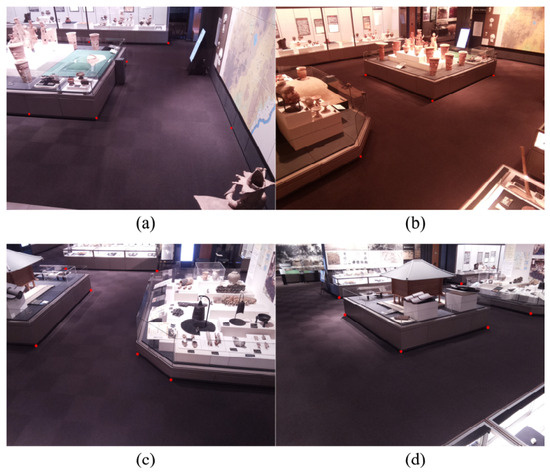
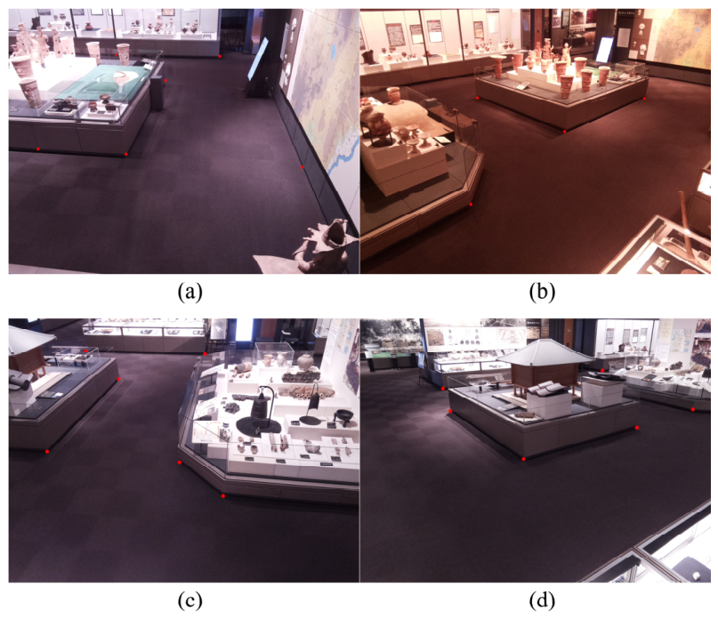
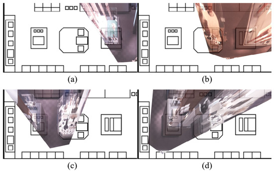
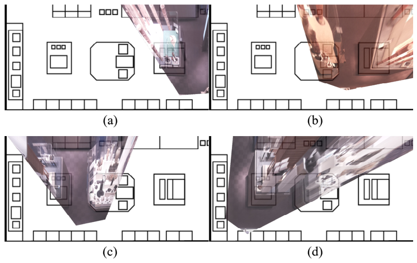
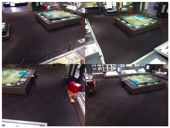
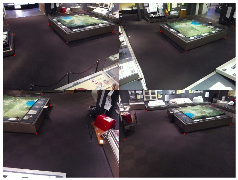
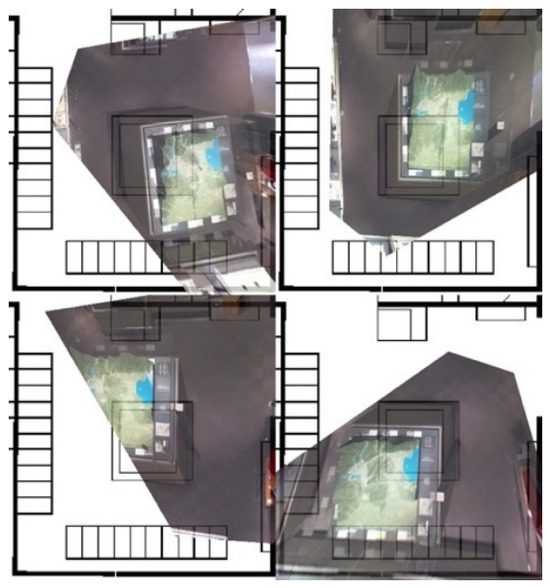
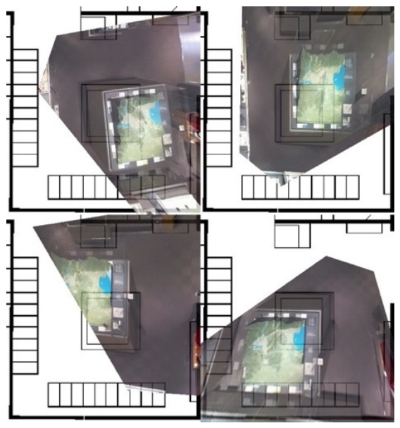
Since bounding box coordinates alone cannot directly identify where a person is located within the museum, a homography transformation was applied to obtain the correspondence between the camera image plane and the floor map plane. Figure 4 and Figure 5 show the input images and their respective projections for the bottom-left configuration (Sensors 8–11). Similarly, Figure 6 and Figure 7 present the sensor images and the resulting homography-based projections for the square-layout configuration in the lower-right area in Figure 3. Homography transformation is an existing method that represents the projective relationship between two-dimensional coordinates on the same plane using a 3 × 3 matrix $H$, and the relationship between image coordinates $(x,y)$ and floor map coordinates $(X,Y)$ is expressed by the following equation using homogeneous coordinates.

$$\left[\begin{array}{c}sX\\ sY\\ s\end{array}\right]=H\left[\begin{array}{c}x\\ y\\ 1\end{array}\right]$$

(1)

Figure 4. Image set captured by (a) Sensor 8, (b) Sensor 9, (c) Sensor 10, and (d) Sensor 11. The red dots in the photos indicate the reference points used to calculate the homography matrix.

Figure 5. Camera images projected onto the floor map for (a) Sensor 8, (b) Sensor 9, (c) Sensor 10, and (d) Sensor 11.

Figure 6. Sensor images captured in the square-layout configuration of the lower-right area in the museum space in Figure 3. The red dots in the photos indicate the reference points used to calculate the homography matrix.

Figure 7. Camera images of the square-layout configuration projected onto the floor map.

Here, $s$ is a scale factor. The homography matrix $H$ is estimated using pairs of corresponding points on the camera image and the floor map. In this study, at least four corresponding point pairs on the image plane and the floor map plane were manually specified, and the homography matrix was calculated using the Direct Linear Transformation (DLT) method based on least squares. Using the calculated homography matrix, the four vertices of the bounding box of a detected person are projected onto the floor map, and the midpoint of the two points corresponding to the bottom edge is calculated to estimate the foot position of the person. Figure 5 shows examples of camera images projected onto the floor map using the estimated homography matrices. Through this process, visitor positions are reconstructed in the floor map coordinate system and can be used for spatiotemporal behavior analysis. The corresponding points are selected using feature points existing on the floor surface of the exhibition space, if they lie on the same plane. In this stage, homography transformation is performed independently for each sensor. The projected visitor positions are reconstructed separately within each sensor’s field of view, and no cross-sensor integration is applied at this step.

3.5. Heatmap Generation and Visitor Flow Visualization

In this study, heatmaps are used to intuitively and quantitatively visualize spatiotemporal behaviors of visitors. Unlike the independent position reconstruction described in Section 3.4, the heatmaps are generated by integrating projected visitor positions obtained from multiple sensors onto a unified floor-map coordinate system. A heatmap represents the frequency or density of visitors at each spatial location as color intensity and is effective for understanding congestion conditions and stay tendencies. Let $\left(x_i{,y}_i\right)$ denote the projected floor-map coordinates of the detected foot position of the $i$-th visitor obtained through homography transformation. The set of all detected visitor positions at time $t$ is defined as $P_t=\left\{\left(x_i\left(t\right),y_i\left(t\right)\right)\right\}$.

To visualize spatial congestion conditions at each time, we generated density heatmaps. To capture density variations of visitors, detections of their spatial positions within a rolling time window of length $T$ are considered. Let $t_k$ denote the timestamp at which the spatial positions of visitors are sampled at the $k$-th frame. We define the set of frame IDs to be accumulated for rendering heatmaps at the sampling time $t$ as:

$$S\left(t\right)=\left\{k\right|t-T\le t_k\le t\}.$$

(2)

The short-term density function $D(x,y,t)$ at an arbitrary floor-map coordinate $(x,y)$ and the time $t$ is defined as:

$$D(x,y,t)=\sum _i\sum _{k\in S\left(t\right)}G\left(x-x_i\left(t_k\right),y-y_i\left(t_k\right)\right),$$

(3)

where $G\left(\cdot \right)$ is a Gaussian kernel:

$$G(x,y)=exp(-{\displaystyle \frac{x^2+y^2}{2{\sigma }^2}}).$$

(4)

Here, $\sigma$ controls the spatial spread (bandwidth) of the density distribution. In this study, $\sigma =25$ (in pixel) was adopted as the experimentally determined bandwidth parameter. This formulation can be interpreted as a computationally efficient approximation of kernel density estimation (KDE).

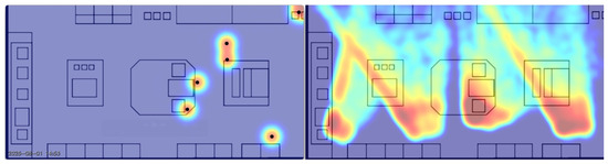
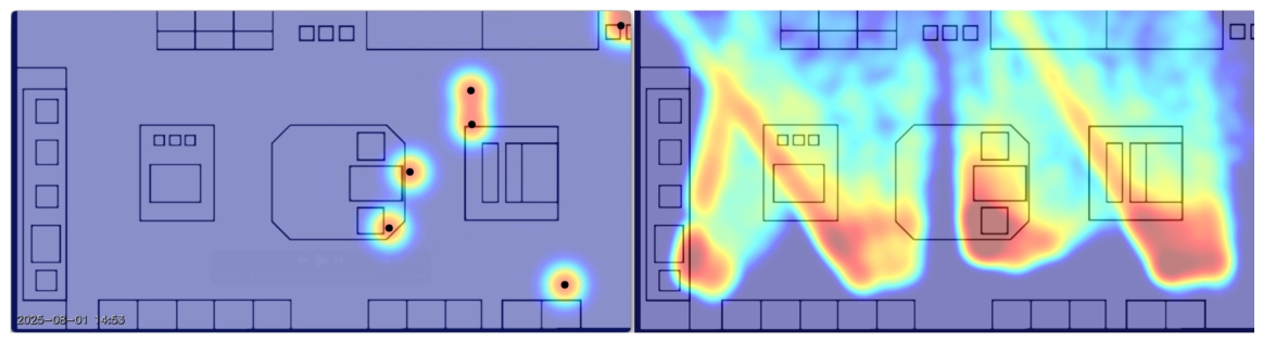
Using the density heatmap allows capturing visitor behavior at different temporal scales. We generate short-term heatmaps by setting $T=10$ min, and long-term heatmaps by setting $T=1$ month. The short-term heatmaps reflect local congestion conditions at a given moment, whereas the long-term heatmaps reveal global behavioral tendencies accumulated over an extended period. This dual-scale visualization framework supports immediate situational awareness in exhibition management while also enabling long-term quantitative evaluation of exhibition layouts. As shown in Figure 8, the heatmap on the left highlights short-term congestion patterns at a specific time, whereas the heatmap on the right reveals long-term stay tendencies and frequently traversed paths.

Figure 8. Comparison of short-term and long-term heatmaps. (Left): short-term density heatmap. (Right): long-term heatmap accumulated over the observation period. Note that high-density areas are shown in warm colors and low-density areas are shown in cool colors in the heatmaps.

3.6. Movement Pattern Visualization

Movement patterns are visualized using a trail-based representation within the rolling time window $S\left(t\right)$ defined in Section 3.5, where a time-dependent fading weight is applied to emphasize recent trajectories. Let ${\tau }_k=t-t_k$ denote the elapsed time since detection. The opacity weight function is defined with the window of time length $T$ as:

$$w({\tau }_k)=\max (0,1-{\displaystyle \frac{{\tau }_k}{T}}).$$

(5)

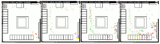
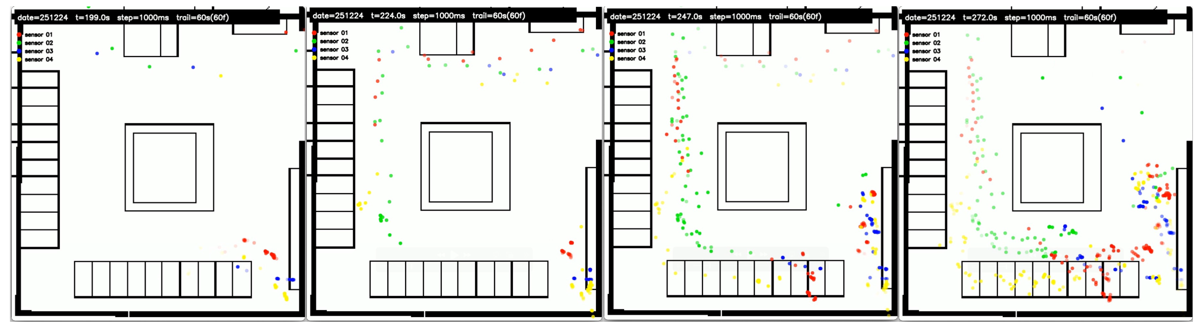
This linear decay function gradually reduces the visual intensity of older trajectory points and ensures that positions older than $T$ are not rendered. Figure 9 shows temporal snapshots of visitors’ spatial positions, captured by four sensors in the second square-layout configuration. Note that the associated color intensity values at the positions are adjusted in proportion to the elapsed time from the present, as described above.

Figure 9. Animation frames of visitor movement patterns. The locations of the visitors, as detected by the four sensors, are labeled with the colors red, blue, green, and yellow, respectively.

We can also compile these visitors’ locations into spatiotemporal density heatmaps.

As before, we control the density $D$ at each position $(x,y)$ in the exhibition space based on the elapsed time from the present $t$ as follows:

$$D(x,y,t)=\sum _i\sum _{k\in S\left(t\right)}w\left({\tau }_k\right)\cdot G(x-x_i(t_k),y-y_i(t_k\left)\right)$$

(6)

Unlike the uniform weighting adopted in the density heatmap in Equation (3), the linear decay function $w\left({\tau }_k\right)$ emphasizes recent motion dynamics and temporal order while preventing visual clutter. Refer to the example in Figure 9.

4. Results

This section demonstrates the results obtained through this study. More specifically, Section 4.1 and Section 4.2 present the spatiotemporal analysis of visitor flows in the first bottom-left configuration, while Section 4.3 shows the trail-based movement patterns of visitors in the second square-layout configuration.

4.1. Results of Spatiotemporal Distribution

In this study, the spatiotemporal positions of visitors were collected from four sensors, selected from the 15 installed in the museum, over approximately three months, from August to October 2025. The total number of analyzed frames was 97,124, of which 37,062 contained at least one person, corresponding to approximately 38.2% of all frames. The total number of detected bounding boxes was 77,359. These values provide an overview of the scale of the dataset used for subsequent spatial and temporal analysis.

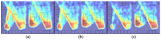
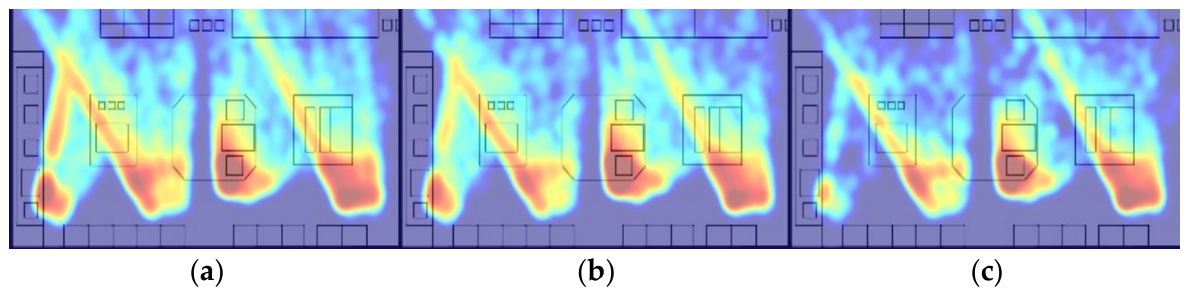
To understand the spatial distribution of visitor behavior, specifically in the bottom-left configuration, long-term heatmaps were generated monthly from August to October 2025. Figure 10 shows the monthly long-term heatmaps of visitor flow for August, September, and October. As a result, a tendency for visitors to stay in specific areas of the exhibition room was observed in all months. In particular, the area covered by Sensor 9 consistently exhibited a high detection frequency throughout the entire period, with a higher detection density than other sensor areas. On the other hand, although a certain number of frames contained detected persons in areas covered by Sensors 10 and 11, high-density stay areas were limited on the long-term heatmaps. This suggests that these areas primarily serve as passageways. The area covered by Sensor 8 showed an intermediate distribution between these two patterns, and changes in staying behavior over the course of the day were observed. When comparing August, September, and October, the locations where visitors stayed did not change significantly across months, and similar spatial distributions were observed repeatedly. This suggests that spatial bias in visitor behavior is not due to temporary factors but is strongly influenced by the structure of the exhibition space and exhibit placement.

Figure 10. Monthly heatmaps of visitor flow: (a) August, (b) September, and (c) October. High-density areas are shown in warm colors, and low-density areas are shown in cool colors.

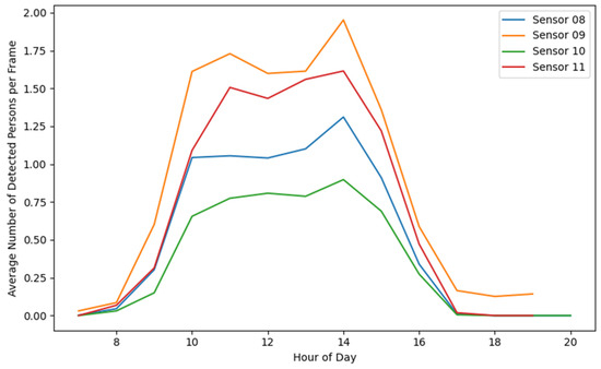
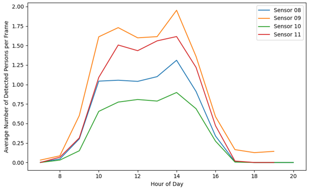
To analyze temporal characteristics of visitor behavior, an analysis was conducted using time information recorded in the presence data from August to October 2025. Detection results for each frame were aggregated along the time axis, and temporal variations in visitor numbers were evaluated. As a result, both the number of frames in which persons were detected and the number of detected bounding boxes varied significantly across time of day. In particular, the maximum number of detected persons per frame varied widely across sensors, with Sensors 8 and 9 exhibiting higher values than the others. In contrast, Sensors 10 and 11 exhibited a few frames with detected persons, but the number of detected persons per frame was relatively low and showed little temporal variation. These results quantitatively indicate that visitor concentration occurs in specific sensor areas and at specific times. Furthermore, similar temporal patterns were observed in August, September, and October, confirming the reproducibility of the temporal distribution of visitor behavior across months. Figure 11 shows the average number of detected visitors per frame for each time and sensor. Across all sensors, the number of detected visitors increased from the morning, peaked around 14:00, and then decreased in the evening.

Figure 11. Average number of detected visitors per each sensor over time (August–October 2025).

4.2. Hypotheses on Visitor Flows

In this section, hypotheses regarding visitor flows within the museum are presented based on the numerical results and visualization results shown in Section 4.1. These hypotheses indicate possibilities derived from the observed data and do not directly determine visitors’ intentions or psychology. First, in the long-term heatmaps, the area where Sensor 9 was installed consistently exhibited high detection density throughout the three-month period. In addition, the numerical results indicate that this sensor recorded a large number of detected bounding boxes. From these results, it can be concluded that the exhibits installed in this area are likely to attract visitors’ interest and induce longer stays. On the other hand, in the areas where Sensors 10 and 11 were installed, although a certain number of person detections were observed, high-density staying areas were limited in the long-term heatmaps. Furthermore, in the temporal analysis results, these sensors exhibited relatively low average numbers of detected persons per frame and small temporal variations. These results suggest that these areas primarily function as movement paths for visitors. In addition, from the time-of-day analysis results shown in Figure 11, it was confirmed that, across all sensors, the number of visitors increased from the morning, peaked around 14:00, and then decreased toward the evening. This temporal variation exhibited similar tendencies in August, September, and October, confirming reproducibility across months. These results suggest that the temporal distribution of visitor behavior is strongly influenced not by temporary events or accidental factors, but by structural factors such as museum opening hours and exhibition configuration. Overall, these hypotheses suggest that spatial and temporal biases in visitor behavior are closely related to the structure of the exhibition space and the placement of exhibits. These findings have the potential to serve as fundamental indicators for the quantitative evaluation of exhibition layouts and for the consideration of exhibit placement improvements.

4.3. Analysis of High-Temporal-Resolution Movement Patterns

In addition to the minute-level density analysis, we conducted movement visualization within the second square-layout configuration. Specifically, in this case, we recorded visitors’ spatiotemporal behavior as videos and extracted frames at 1-s intervals. This high-temporal-resolution data enables the observation of dynamic behaviors that are often obscured in long-term heatmaps.

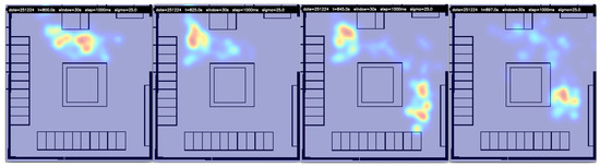
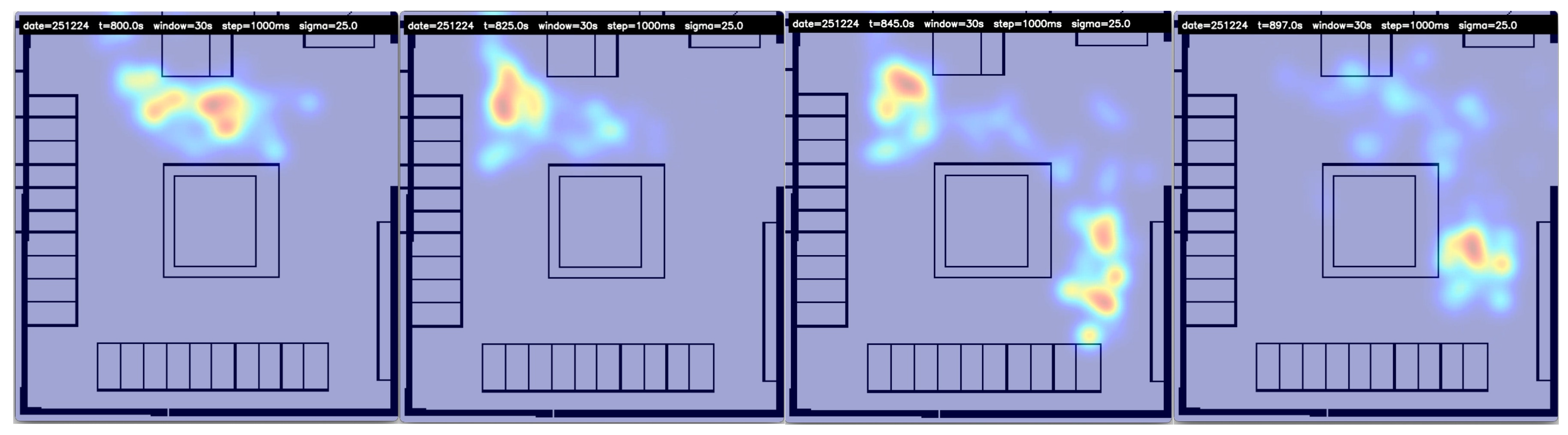
Figure 12 presents the sequence of frames used to animate the trail-based visualization of visitors’ behavior. The resulting trail-based visualization reveals clear directional convergence toward specific interactive exhibition terminals. Unlike traditional exhibits, these hands-on installations function as “behavioral anchors” within the layout, inducing repeated short-term stops and localized trajectory accumulation. While the long-term heatmaps (Section 4.1) identify these areas as high-density zones, the second-level trail analysis clarifies the engagement process: visitors do not merely pass through but actively approach, pause, and circulate around these interactive elements.

Figure 12. 1-s frame sequence for trail-based visualization. High-density areas are shown in warm colors, and low-density areas are shown in cool colors.

From a curatorial perspective, these findings provide a quantitative basis for evidence-based spatial redesign. For instance, the concentration of flow around specific terminals suggests that strategically placing such interactive elements can guide visitor circulation or distribute congestion more evenly across the gallery. By integrating high-temporal-resolution trails with long-term density evaluation, this framework provides curators with deeper insights into how exhibit characteristics directly shape the dynamic movement and engagement of visitors.

5. Conclusions

In this study, a method for quantitatively analyzing and visualizing visitor flows was proposed using spatiotemporal behaviors of visitors acquired from multiple camera sensors installed in a museum. From a privacy perspective, images were not used; instead, visitor positions were estimated from bounding box coordinates and projected onto a floor map via a homography, thereby reconstructing the spatial and temporal characteristics of visitor behavior. Analysis of real data collected over three months, from August to October 2025, confirmed a tendency for visitor stay behavior to concentrate in specific areas of the exhibition room. In addition, temporal analysis revealed a common pattern in which visitor numbers increased from the morning, peaked around 14:00, and then decreased in the evening. These tendencies were consistent across months, suggesting that visitor behavior is closely related to exhibition space structure and exhibit placement. A key feature of this study is that visitor behavior within a museum can be quantitatively evaluated using a low-cost sensor configuration and analysis based solely on bounding box information. The proposed method is expected to provide objective criteria for spatial design to improve exhibition layouts and alleviate congestion.

On the other hand, several technical issues still remain. This analysis did not perform visitor identification or tracking and therefore could not directly evaluate the long-term behavior of the same person. In addition, attribute information, such as visitor age group and interests, was not included, and background factors influencing behavior were not sufficiently considered. Future work includes more detailed analysis of stay time and movement routes by introducing person-tracking methods, as well as comparisons of visitor flow before and after changes in exhibition content. Furthermore, by integrating analysis with other types of sensor data that can be acquired, it is desirable to develop methods that capture visitor behavior from multiple perspectives.

References

- Yalowitz, S.S.; Bronnenkant, K. Timing and Tracking: Unlocking Visitor Behavior. Visit. Stud. 2009, 12, 47–64. [Google Scholar] [CrossRef] [Scilit]
- Zancanaro, M.; Kuflik, T.; Boger, Z.; Goren-Bar, D.; Goldwasser, D. Analyzing Museum Visitors’ Behavior Patterns. In User Modeling 2007; Conati, C., McCoy, K., Paliouras, G., Eds.; Lecture Notes in Computer Science; Springer: Berlin/Heidelberg, Germany, 2007; Volume 4511, pp. 238–242. [Google Scholar] [CrossRef] [Scilit]
- Strohmaier, R.; Sprung, G.; Nischelwitzer, A.; Schadenbauer, S. Using Visitor Flow Visualization to Improve Visitor Experi-ences in Museums and Exhibitions. In Proceedings of the Museums and the Web 2015, Chicago, IL, USA, 8–11 April 2015. [Google Scholar]
- Shapiro, B.R.; Hall, R.P.; Owens, D.A. Developing and Using Interaction Geography in a Museum. Int. J. Comput.-Support. Collab. Learn. 2017, 12, 377–399. [Google Scholar] [CrossRef] [Scilit]
- Yoshimura, Y.; Krebs, A.; Ratti, C. Noninvasive Bluetooth Monitoring of Visitors’ Length of Stay at the Louvre. IEEE Pervasive Comput. 2017, 16, 26–34. [Google Scholar] [CrossRef] [Scilit]
- Muramatsu, S.; Kasano, E.; Motohashi, Y.; Sato-Shimokawara, E.; Chan, R.Y.Y.; Yamaguchi, T. Estimating Indoor Behavior Using Sensor Fusion with BLE Beacons and Wearable Devices for Information Presentation. In Proceedings of the 2019 16th International Conference on Ubiquitous Robots (UR), Jeju, Republic of Korea, 24–27 June 2019; pp. 236–239. [Google Scholar] [CrossRef] [Scilit]
- Umezu, N.; Koizumi, S. Visitor Counting in a Museum with a 2D LiDAR Sensor. In Proceedings of the 2023 IEEE 12th Global Conference on Consumer Electronics (GCCE), Nara, Japan, 10–13 October 2023; pp. 73–75. [Google Scholar] [CrossRef] [Scilit]
- Umezu, N.; Koizumi, S.; Nakagawa, K.; Nishida, S. Potential of Low-Cost Light Detection and Ranging (LiDAR) Sensors: Case studies for enhancing visitor experience at a science museum. Electronics 2023, 12, 3351. [Google Scholar] [CrossRef] [Scilit]
- Saito, Y.; Okuzumi, J.; Suzuki, N. Comparison of GPS Data Acquisition for Open Air Museums by Two APIs. In Proceedings of the 2022 IEEE International Conference on Artificial Intelligence and Virtual Reality (AIVR), Online, 14–16 December 2022; pp. 248–251. [Google Scholar] [CrossRef] [Scilit]
- Serasidis, V.; Sofianidis, I.; Margaritis, G.; Sad, C.; Konstantakos, V.; Siozios, K. ICE: A Low-Cost IoT Platform Targeting Real-Time Anonymous Visitors Flow Tracking at Museums. In Proceedings of the 2023 IEEE 32nd International Symposium on Industrial Electronics (ISIE), Helsinki, Finland, 19–21 June 2023; pp. 1–6. [Google Scholar] [CrossRef] [Scilit]
- Ferrato, A.; Limongelli, C.; Mezzini, M.; Sansonetti, G. Using Deep Learning for Collecting Data about Museum Visitor Behavior. Appl. Sci. 2022, 12, 533. [Google Scholar] [CrossRef] [Scilit]
- Breitner, A.R.; Bandung, Y. Calculation of Museum Collections Popularity Using Detection and Tracking of Visitors from Surveillance Cameras in Low Light Conditions. In Proceedings of the 2024 International Seminar on Intelligent Technology and Its Applications (ISITIA), Mataram, Indonesia, 24–25 July 2024; pp. 316–321. [Google Scholar] [CrossRef] [Scilit]
- Centorrino, P.; Corbetta, A.; Cristiani, E.; Onofri, E. Managing Crowded Museums: Visitors Flow Measurement, Analysis, Modeling, and Optimization. J. Comput. Sci. 2021, 53, 101357. [Google Scholar] [CrossRef] [Scilit]
- Takahashi, S.; Nishidate, Y.; Kohira, Y.; Yoshioka, R. Visualizing Maps of Visitors’ Interest for Museum Exhibits with Single-Board Computers. In Proceedings of the 2023 27th International Conference Information Visualisation (IV), Tampere, Finland, 3–7 July 2023; pp. 64–70. [Google Scholar] [CrossRef] [Scilit]
- Yanada, A.; Miyaoka, E.; Yoshioka, R. Knowledge Experience Model for Designing Data Exploration Tools in Museums. In Proceedings of the 2023 4th Asia Service Sciences and Software Engineering Conference (ASSE ‘23), New York, NY, USA, 27–29 October 2023; pp. 29–32. [Google Scholar] [CrossRef] [Scilit]
- Tamahashi, T.; Yoshioka, R.; Hoshino, T. UI Method to Support Knowledge Creation in Hybrid Museum Experience. In Proceedings of the 2021 IEEE 14th International Symposium on Embedded Multicore/Many-Core Systems-on-Chip (MCSoC), Singapore, 20–23 December 2021; pp. 292–295. [Google Scholar] [CrossRef] [Scilit]
- Hoshino, T.; Yoshioka, R. A Software Design Method for Creation and Utilization of Experiential Knowledge. In Proceedings of the 2022 International Conference on Electrical, Computer and Energy Technologies (ICECET), Prague, Czech Republic, 20–22 July 2022; pp. 1–6. [Google Scholar] [CrossRef] [Scilit]
- Philippopoulos, P.I.; Drivas, I.C.; Tselikas, N.D.; Koutrakis, K.N.; Melidi, E.; Kouis, D. A Holistic Approach for Enhancing Museum Performance and Visitor Experience. Sensors 2024, 24, 966. [Google Scholar] [CrossRef] [Scilit] [PubMed]
- Primadani, T.I.W.; Pramono, A.; Wijaya, I.B.A.; Agustina, I.A. Visitor’s Response to the Technology-Based Interactive Displays and its Placement at the Museum in East Java. In Proceedings of the 2021 3rd International Conference on Cybernetics and Intelligent System (ICORIS), Makasar, Indonesia, 25–26 October 2021; pp. 1–5. [Google Scholar] [CrossRef] [Scilit]
- Nishidate, Y.; Kohira, Y.; Takahashi, S.; Yoshioka, R. Precise Detection of Changes in Relatively Static Environments for Single-Board Computers. In Proceedings of the 2023 14th IIAI International Congress on Advanced Applied Informatics (IIAI-AAI), Koriyama, Japan, 8–13 July 2023; pp. 57–62. [Google Scholar] [CrossRef] [Scilit]
- Nishidate, Y.; Kohira, Y.; Takahashi, S.; Yoshioka, R. Enhanced Image Differencing for Precise Change Detection in Static Environments. Inf. Eng. Express 2024, 10. [Google Scholar] [CrossRef] [Scilit]
Disclaimer/Publisher’s Note: The statements, opinions and data contained in all publications are solely those of the individual author(s) and contributor(s) and not of MDPI and/or the editor(s). MDPI and/or the editor(s) disclaim responsibility for any injury to people or property resulting from any ideas, methods, instructions or products referred to in the content. |
© 2026 by the authors. Licensee MDPI, Basel, Switzerland. This article is an open access article distributed under the terms and conditions of the Creative Commons Attribution (CC BY) license.