


Abstract
The rapid and non-destructive determination of sodium chloride (NaCl) in aqueous solutions is critical to food-process monitoring, pharmaceutical manufacturing, and the chlor-alkali and desalination industries. This study presents a method based on Raman spectroscopy (785 nm; 350–2000 cm−1) combined with partial least squares regression (PLS-R) for estimating NaCl in simple aqueous solutions at concentrations between 0.02 and 4.0 mol·L−1. Since Na+ and Cl− ions lack intrinsic Raman modes, the quantification was based on the modifications that ionic solvation induces on the hydrogen-bond network of water, mainly affecting the librational (450–780 cm−1) and H-O-H bending modes (~1640 cm−1). Four preprocessing strategies were systematically evaluated. The model with the combination of asymmetric least squares baseline correction and Savitzky–Golay smoothing (ALS-SG) provided the lowest root mean square error of cross-validation (RMSECV = 0.0608 mol·L−1), requiring only two latent variables (calibration coefficient of determination, R2cal = 0.9990 and cross-validated coefficient of determination, Q2CV = 0.9979). The holdout prediction set (n = 5) yielded a coefficient of determination (R2ext) of 0.9946 and a root mean square error of prediction (RMSEP) of 0.0681 mol·L−1, with an empirical lower limit of reliable prediction of ~0.18 mol·L−1. The holdout samples span 0.04–2.50 mol·L−1, so predictive performance between 2.50 and 4.00 mol·L−1 is supported by calibration and cross-validation only. Given the small size of this set, these figures are reported as a proof-of-concept indication and support the potential of the approach for NaCl monitoring in simple aqueous matrices.
1. Introduction
Sodium chloride (NaCl) is one of the most important inorganic salts in industrial processing, with applications including food preservation, pharmaceutical manufacturing, chlor-alkali electrolysis, and desalination [1,2,3,4,5,6]. In the food industry, its concentration influences curing kinetics, water activity, and the microbiological stability of the product [1,2]. In pharmaceutical production, saline solutions with controlled ionic strength are crucial for isotonicity and, therefore, for patient safety [4]. In the chlor-alkali process, the concentration of the feed brine directly affects current efficiency and the longevity of the ion-exchange membrane [3,5,6]. Meanwhile, desalination and water reuse plants require continuous monitoring of salt rejection to meet regulatory discharge limits. The diversity of these contexts and the sensitivity of the associated variables justify the need for rapid and accurate analytical methods compatible with process monitoring [4,5,6].
Conventional methods for determining chloride or salinity in solution include argentometric titrations, potentiometry with ion-selective electrodes, refractometry, and conductimetry [7,8,9]. Although these techniques offer adequate accuracy under controlled laboratory settings, they present clear limitations for in-line implementation. Wet-chemical titrations require reagent consumption and are prone to operator-dependent endpoint detection. Conductivity measurements are sensitive to temperature and the presence of other ionic species, whereas refractometry loses specificity in multicomponent matrices with co-dissolved solutes. Likewise, selective electrodes can be affected by membrane fouling and calibration drift under industrial operating conditions. Collectively, these limitations motivate the development of non-invasive, reagent-free techniques capable of providing quantitative determination while minimizing sample handling and avoiding direct probe-sample contact.
Raman spectroscopy offers key advantages for this purpose, including molecular specificity, minimal sample preparation, and compatibility with fiber-optic probes for in-line measurement [10,11,12]. While infrared spectroscopy is severely limited in aqueous media due to strong water absorption, Raman scattering is minimally attenuated by the aqueous matrix, making it appropriate for the analysis of solutions. For NaCl solutions, the solvation of Na+ and Cl− ions induces perturbations in the hydrogen-bond network of water, which manifest as variations in intensity and spectral profile in the O-H stretching (~3400 cm−1) [13,14] and bending (~1640 cm−1) bands. Although these variations, considered in isolation, are of small magnitude and concentration-dependent, they contain multivariate information that can be extracted using chemometric methods.
Partial least squares regression (PLS-R) has become established as the reference chemometric approach for extracting quantitative information from spectroscopic data characterized by band overlap or low contrast [15,16,17]. The method constructs decompositions into latent variables that maximize the covariance between the spectral variables and the reference variable, thereby providing stable predictions even in the presence of collinearity. The integration of PLS-R with Raman spectroscopy has been documented for pharmaceutical solutions, food matrices, and bioprocess monitoring applications [18,19,20]. Spectral preprocessing plays a relevant auxiliary role: Savitzky–Golay (SG) smoothing attenuates high-frequency detector noise while preserving band position and shape [21], whereas asymmetric least squares (ALS) baseline correction, implemented using Whittaker-type penalized smoothers [22], eliminates broadband contributions associated with fluorescence and instrumental drift, which would otherwise increase model complexity and compromise its predictive performance. Available reviews on vibrational and near-infrared spectral preprocessing agree on the advantages of combining scattering correction, derivative correction, and baseline correction to optimize multivariate calibration models [23]. The feasibility of this approach is supported by chemometric studies of water structure using vibrational spectroscopy, where changes in the spectral features of water have been used as indirect probes of molecular interactions and structural transformations in aqueous systems [24].
Raman spectroscopy has been used to determine NaCl in aqueous solutions for several decades. Because monatomic ions have no internal vibrational modes, all such methods rely on the perturbation that ion hydration induces in the spectrum of water. Representative approaches are summarized in Table 1. Early work relied on difference spectroscopy against a pure-water reference [25] or on intensity ratios within the O–H stretching band [13]. Subsequent approaches fitted that band with Gaussian sub-bands and calibrated the resulting intensity ratio against Cl− molarity [26,27], while others applied multivariate or machine-learning models to the same spectral region [28], in one case, alongside a low-wavenumber window but with the spectra normalized to the area of the O–H stretching band [29]. The study closest to the present one combined PLS-R with nine descriptors derived from a three-Gaussian fit of the O–H stretching band within a multi-temperature design [30]. All of these determinations were performed under visible excitation (488–532 nm), for which the O–H stretching band appears within the high-sensitivity range of silicon CCD detectors. Under 785 nm excitation, widely used in fiber-probe systems to reduce fluorescence, the same band appears beyond the detection window of the configuration used in this work. The information available for NaCl quantification is therefore confined to the region below ~2000 cm−1, which contains the librational (450–780 cm−1) and H–O–H bending (~1640 cm−1) bands of water.
Table 1.
Representative Raman-based approaches to the determination of NaCl and chloride in aqueous solution.
Near-infrared approaches coupled with PLS-R, while achieving comparable accuracy, operate on broader spectral features and typically require a greater number of latent variables [31,32,33,34].
However, to the best of our knowledge, no methodology combining Raman spectroscopy with PLS-R for aqueous NaCl solutions has been reported that simultaneously (i) targets the librational (450–780 cm−1) and bending regions (~1640 cm−1) of water; (ii) covers a broad range of industrially relevant NaCl concentrations; (iii) involves a comparison of different preprocessing strategies; and (iv) verifies predictive performance using a holdout prediction set. This study therefore, as the first proof of concept on a simple, controlled NaCl matrix, examines whether the low-wavenumber region alone, without recourse to the O–H stretching band for either measurement or normalization, carries sufficient information for NaCl quantification by PLS-R. A non-destructive quantitative method based on Raman spectroscopy (excitation at 785 nm; range 350–2000 cm−1) coupled with PLS-R was developed for estimating the concentration of NaCl in simple, controlled aqueous NaCl solutions over the range of 0.02 to 4.0 mol·L−1. The effects of SG smoothing and ALS baseline correction on model performance were systematically evaluated, and the resulting model was assessed using Venetian blinds cross-validation over the full calibration range and a holdout prediction set covering 0.04–2.50 mol·L−1. The reported metrics are intended to establish feasibility and to delimit the conditions under which the approach may be developed further.
2. Materials and Methods
2.1. Design of the Sample Set and Preparation of the Solutions
Twenty aqueous sodium chloride solutions were prepared in distilled water to calibrate and assess the PLS-R model. The concentration design comprised twenty distinct steps over the range of 0.02 to 4.0 mol·L−1, with the following specific concentrations: 0.02, 0.04, 0.06, 0.08, 0.10, 0.12, 0.14, 0.16, 0.18, 0.20, 0.40, 0.60, 0.80, 1.0, 1.5, 2.0, 2.5, 3.0, 3.5, and 4.0 mol·L−1. The concentration levels were deliberately distributed with a higher density in the low-concentration region (ten of the twenty levels at or below 0.20 mol·L−1) in order to adequately characterize the most challenging range, where the analytical signal is weakest.
The solutions were prepared under controlled laboratory conditions at 25 ± 0.5 °C. Class A volumetric glassware was used throughout, and the analytical balance and the piston pipettes were calibrated and verified before use according to the internal calibration schedule of the laboratory, with traceability to the certificates issued by the corresponding calibration service. Anhydrous analytical-grade sodium chloride crystals conforming to ACS standards, with a purity of 99.8% (Fermont, Mexico, lot 434262), were used as the solute. The solvent used was distilled water (Wöhler, product W1000, Mexico, lot 25I02; CAS 7732-18-5), with a maximum specific conductivity of 1.0 × 10⁻⁶ Ω−1·cm−1 and a pH of 5.0–7.0 at 25 °C, thereby minimizing the contribution of ionic contaminants. Volumetric glassware was cleaned with a neutral liquid detergent for exclusive laboratory use (Hyclin Plus Neutral, Mexico, Cat. 5342, lot 522684, pH 7.00) diluted to 5% with tap water, followed by three rinses with distilled water and air-drying on a rack at room temperature.
The set of solutions was prepared from a 4.0 mol·L−1 stock solution. The required mass of sodium chloride, calculated for a final volume of 500 mL, was weighed on a previously calibrated and verified analytical balance (Ohaus, Pioneer series, model PX224, Parsippany, NJ, USA; resolution 0.0001 g). The solid was dissolved in a partial volume of distilled water (∼350 mL) heated to 40 °C on a hot plate with a magnetic stirrer until complete dissolution was achieved. The solution was then allowed to cool to ambient temperature, diluted to volume with distilled water, thoroughly mixed, and allowed to equilibrate before use.
All calibration standards were prepared, in a single session, directly from the 4.00 mol·L−1 stock solution by dilution with distilled water. For each standard, the required volume of stock solution was transferred to a 100 mL Class A volumetric flask and diluted to volume. The transferred volume was calculated from the dilution equation C1V1 = C2V2 with C1 = 4.00 mol·L−1 and V2 = 100.00 mL. Each standard therefore required a single dilution step, except for the 4.00 mol·L−1 solution, which was used undiluted. The transferred volumes ranged from 0.50 mL for the most dilute standard (0.02 mol·L−1) to 87.50 mL for the 3.50 mol·L−1 standard. Aliquots were transferred using two variable-volume piston pipettes with calibration and periodic verification: a variable-volume micropipette (ScienceMED, Finland; 100–1000 µL) for the 0.50 mL aliquot of the 0.02 mol·L−1 standard; a macropipette (Transferpette® S Brand, Germany; 1–10 mL) for aliquots between 1.00 and 10.00 mL, corresponding to the 0.04–0.40 mol·L−1 standards; and Class A volumetric pipettes for aliquots above 10 mL, corresponding to the 0.60–3.50 mol·L−1 standards. Once the volumes were transferred, the solutions were diluted to volume and homogenized. The final solutions were stored in airtight polypropylene bottles inside a thermally insulated transport container for 12 h before spectral acquisition to minimize concentration drift due to evaporation.
The reference concentrations used to build and evaluate the models are nominal values obtained from gravimetric and volumetric preparation. The errors reported below therefore express the agreement between the model prediction and the prepared concentration.
2.2. Raman Spectra Acquisition
Raman spectra of the twenty NaCl solutions were acquired using a system consisting of a non-submersible fiber-optic probe mounted on a fixed support, a diode laser source with an excitation wavelength of 785 nm, and a back-thinned spectrometer (Ocean Optics QE65000, Edinburgh, UK) with a full-frame transfer charge-coupled device (FFT-CCD) detector, operated via SpectraSuite software (version 2.0.162, Ocean Optics, Edinburgh, UK). Prior to spectral acquisition, the solutions were homogenized by manual inversion and stabilized for 30 min to ensure thermal equilibrium and bubble dissipation. The solutions were transferred to transparent quartz cuvettes filled to 1 mm below the upper rim. The instrument was powered on 20 to 30 min before measurements to allow stabilization of the diode laser output power.
The cuvettes were placed on a movable plate, and the distance between the liquid surface and the fiber-optic probe was adjusted to 4 mm to enable backscattering geometry measurements. The acquisition spectral range spanned from 350 to 2000 cm−1, with a resolution of 17 cm−1 and a digital sampling interval of approximately 2.56 cm−1. Dark background correction was applied in the software, and five averaged scans were performed with a 10 s integration time at a laser power of 30 mW; laser power was kept fixed for all 20 samples so that excitation conditions would not contribute to between-sample variability. Spectra of each sample were acquired in triplicate in random order at an ambient temperature of approximately 25 °C; spectra containing cosmic ray artifacts detected during acquisition were discarded and reacquired. Additionally, Raman spectra of the distilled water used to prepare the solutions were acquired as an instrumental quality-control measurement. All the spectra reported were acquired in a single session on the same day. The output files were stored in text format and consolidated into a database. The representative Raman spectrum of each sample was obtained by averaging the three replicate measurements.
2.3. Spectral Preprocessing
In order to evaluate different chemometric modeling scenarios, the raw spectra were subjected to four preprocessing strategies: (1) baseline correction using the ALS method; (2) smoothing with the SG filter; (3) ALS–SG sequential combination; and (4) ALS–SG combination followed by standard normal variate (SNV) normalization. All preprocessing steps were implemented in Python (version 3.13.7) code.
2.3.1. Baseline Correction by Asymmetric Least Squares
Baseline correction was performed using the asymmetric least squares (ALS) method, implemented as a Whittaker-type penalized smoother [22,35]. The method estimates the baseline by minimizing a two-term objective function. The first term measures the fidelity of the baseline to the measured spectrum, computed as the sum of the squared differences between measured and estimated intensities at each spectral point, each weighted individually. The second term penalizes the roughness of the baseline, computed as the sum of the squared second-order differences in the estimated baseline, and is scaled by a smoothing parameter λ that determines the relative importance of the two terms: larger values of λ yield smoother baselines.
The weights of the fidelity term are assigned asymmetrically and updated iteratively. At each iteration, spectral points lying above the current baseline estimate receive a weight equal to the asymmetry parameter p, while points lying below receive a weight of 1 − p. Since p is small, points below the baseline are weighted far more heavily, and the estimate is drawn toward the lower envelope of the spectrum. This asymmetric weighting enables the removal of broadband contributions associated with fluorescence and instrumental drift while preserving the narrower spectral features of interest [35].
Parameters were established for each spectrum independently through a grid search over λ (1 × 10³, 5 × 10³, 1 × 10⁴, 5 × 10⁴, 1 × 10⁵, 5 × 10⁵, 1 × 10⁶, 3 × 10⁶, and 5 × 10⁶) and p (0.001, 0.005, 0.01, 0.02, and 0.05). For each combination the roughness of the resulting baseline was evaluated as the sum of its squared second-order differences; that is, the penalty term described above, and the combination minimizing this quantity was retained. The values obtained from this procedure were within the ranges commonly reported for Raman spectroscopy (λ = 105, p = 0.001) and applied consistently to all spectra. All corrected spectra were verified by visual inspection.
2.3.2. Savitzky–Golay Smoothing Filter
Spectral smoothing was performed using the SG filter [21], employing a second-degree polynomial and an 11-point window. These parameters were determined by calculating the signal-to-noise ratio (SNR) for each spectrum and assessing the overall improvement after applying the filter [36]. The selected window size effectively attenuated high-frequency detector noise without compromising band position or spectral shape [21,36]. Only the fifteen calibration spectra were used for this selection; the resulting filter was then applied unchanged to the five holdout spectra.
2.3.3. Normalization by Standard Normal Variate
SNV normalization was applied as the final preprocessing step in the fourth scenario [23,37]. The SNV transformation centers and scales each spectrum individually using its mean and standard deviation, thereby removing multiplicative scattering and baseline variations that are independent of the analyte concentration [37]. The implementation followed the procedure described by Barnes et al. [37], recognized as a standard technique for correcting scattering effects in vibrational spectroscopy [23].
2.4. Development of the PLS-R Model
For each of the four preprocessing scenarios, a PLS-R model was developed [15,16]. The models were fitted using the nonlinear iterative partial least squares algorithm (NIPALS) [15], in which the predictor matrix X corresponded to the spectral intensities (a.u.) and the response vector Y to the NaCl concentration (mol·L−1) [17]. For model construction, the dataset of 20 samples was divided into a training subset of 15 samples and a holdout prediction subset of 5 samples. The partition was performed manually, and no spectral selection algorithm was applied. Given the limited number of samples, the five holdout samples (M2, M4, M9, M13, and M17, at 0.04, 0.08, 0.18, 0.80, and 2.50 mol·L−1) were selected to span the low-, intermediate-, and high-concentration regions in proportion to the number of samples available in each region, thereby preventing the extreme values of the working range from being assigned entirely to one subset. This partition was fixed prior to preprocessing optimization and latent variable selection, and was kept identical across the four preprocessing scenarios, so that the comparison between them was not influenced by sample allocation.
The optimal number of latent variables (LVs) was selected by evaluating models with one to five components and identifying the configuration that minimized the root mean square error of cross-validation (RMSECV) [38]. A Venetian blinds cross-validation scheme with k segments (k = 3) was used according to Ezenarro and Schorn-García [39]. The calibration samples were arranged in ascending order of NaCl concentration, and each sample was assigned sequentially to one of the segments. This produced three interleaved segments of five samples each, so that every segment spanned the full calibration range. Each sample served as a test sample exactly once, and each intermediate model was fitted on the remaining ten samples. No randomization was applied at any stage, making the partition fully deterministic, defined solely by concentration order, and exactly reproducible. Because the scheme is deterministic and concentration-ordered, each test sample retains its nearest concentration neighbors in the training set; the resulting cross-validation metrics were therefore used for model selection and interpreted as an upper-bound estimate of predictive performance, with the holdout prediction set providing an additional assessment. The metrics used to compare preprocessing configurations and to characterize the resulting models were the calibration coefficient of determination (R2cal), cross-validated coefficient of determination (Q2CV), RMSECV, residual predictive deviation (RPD), and bias [38,40]. The RPD was calculated as the ratio of the standard deviation of the reference concentrations of the calibration set (SDcal) to the RMSECV, and, because RPD assumes an approximately normal distribution of the reference values and is sensitive to outliers, the ratio of performance to interquartile distance (RPIQ) was also computed, using the interquartile range of the calibration set in place of the standard deviation. Bias was defined as the mean of the prediction errors over the sample set, with the error of each sample computed as the reference concentration minus the predicted concentration. Under this sign convention, a positive bias indicates systematic underestimation of the reference concentration by the model, whereas a negative bias indicates systematic overestimation.
The relevance of spectral variables was assessed using variable importance in projection (VIP) values [41], calculated from the weights, scores and loadings of the PLS-R model. Following the usual interpretive convention, spectral variables with VIP ≥ 1.0 were regarded as influential for the calibration model.
A permutation test (n = 999) [42] was applied to assess whether the observed relationship could be reproduced by random reassignment of the reference concentrations, in which the response variable was randomly permuted at each iteration and the coefficient of determination (Q2) statistic was recalculated under the same cross-validation scheme. The distribution of the permuted coefficient of determination (Q2perm) values was compared with the Q2CV of the original model to rule out the presence of spurious correlations [42]. As an additional step to the permutation test, the empirical p-value was computed as p = (r + 1)/(n + 1), where r is the number of permutations whose Q2perm exceeded the Q2CV of the original model, so that the minimum attainable value with n = 999 is 0.001 [43].
2.5. Holdout Prediction Set
The final PLS-R model was applied to the holdout prediction set of 5 samples (0.04, 0.08, 0.18, 0.80 and 2.5 mol·L−1) reserved during training in order to obtain a first indication of its prediction error [38]. These five samples were reserved from the same preparation batch and acquisition session as the calibration set; the reserved samples span 0.04 to 2.50 mol·L−1. Prediction errors were defined as the reference concentration minus the predicted concentration, and the root mean square error of prediction (RMSEP), standard error of prediction (SEP), bias, coefficient of determination (R2ext), and RPD index were calculated on this basis [38,40]. For consistency with the cross-validation values, the RPD reported for the holdout set uses SDcal as the numerator, divided by the RMSEP.
3. Results and Discussion
3.1. Spectral Characterization and Preprocessing
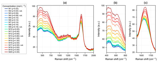
The raw spectra of the twenty NaCl solutions, with concentrations between 0.02 and 4.00 mol∙L−1, acquired in the range of 350 to 2000 cm−1, are shown in Figure 1. The spectra share the general features of liquid water, in which the contribution of the librational modes of the hydrogen-bond network is observed in the range of 450 to 780 cm−1 [44], superimposed on fluorescence background effects, while that of the H-O-H bending band is observed centered at ~1640 cm−1 [45].
Figure 1.
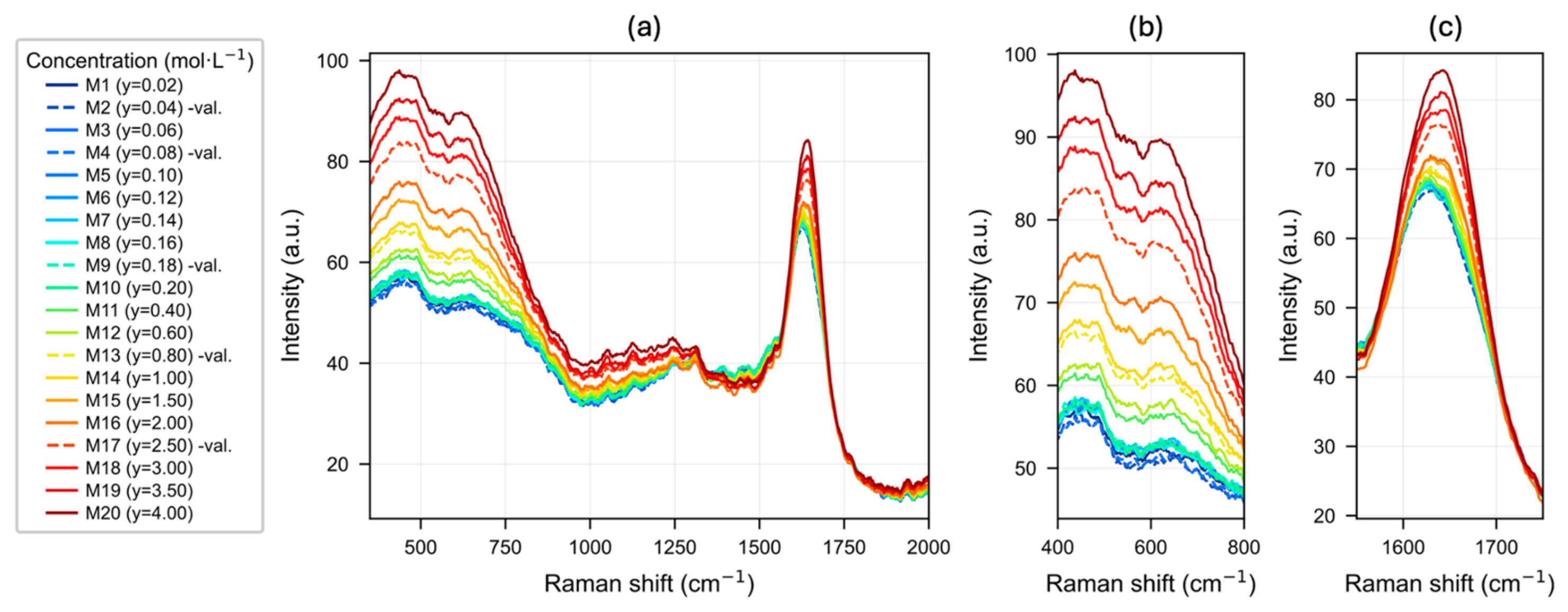
(a) Raman spectra of aqueous sodium chloride (NaCl) solutions without preprocessing, in the range of 350 to 2000 cm−1, acquired using 785 nm laser excitation. The 20 samples are shown as follows: solid lines correspond to the calibration set (n = 15) and dashed lines correspond to the holdout prediction set (n = 5; samples M2, M4, M9, M13, and M17). The color of each spectrum indicates the increasing order of NaCl concentration, from blue (lowest) to red (highest). (b) Magnified view of the representative range of the 450–780 cm−1 region and (c) magnified view of the region around 1640 cm−1, clearly illustrating the increasing trend in intensity with increasing solution concentration (>0.20 mol·L−1).
This characteristic pattern of water shows a systematic increase in intensity in response to increasing concentration: the low-frequency region (450–780 cm−1) exhibits an increase in signal intensity with NaCl concentration, such that the higher-concentration samples (M18–M20, red lines) show substantially higher intensities than the dilute samples (M1–M10, blue lines). However, it is important to note that in the very-low-concentration subrange (0.02–0.20 mol∙L−1), the systematic trend becomes less evident. The overall progressive increase reflects how the solvation of Na+ and Cl− ions perturbs the solvent structure proportionally to the concentration, generating the indirect analytical signal that supports the proposed quantitative model. The five samples of the holdout set (M2, M4, M9, M13, and M17; dashed lines) are distributed across the concentration design, covering its low, intermediate, and high portions.
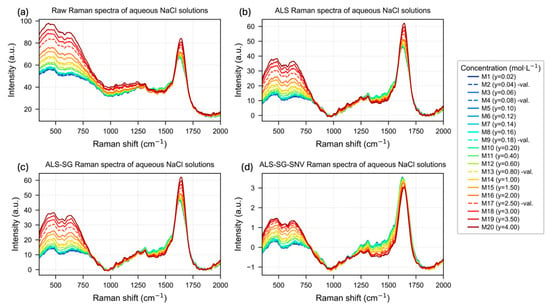
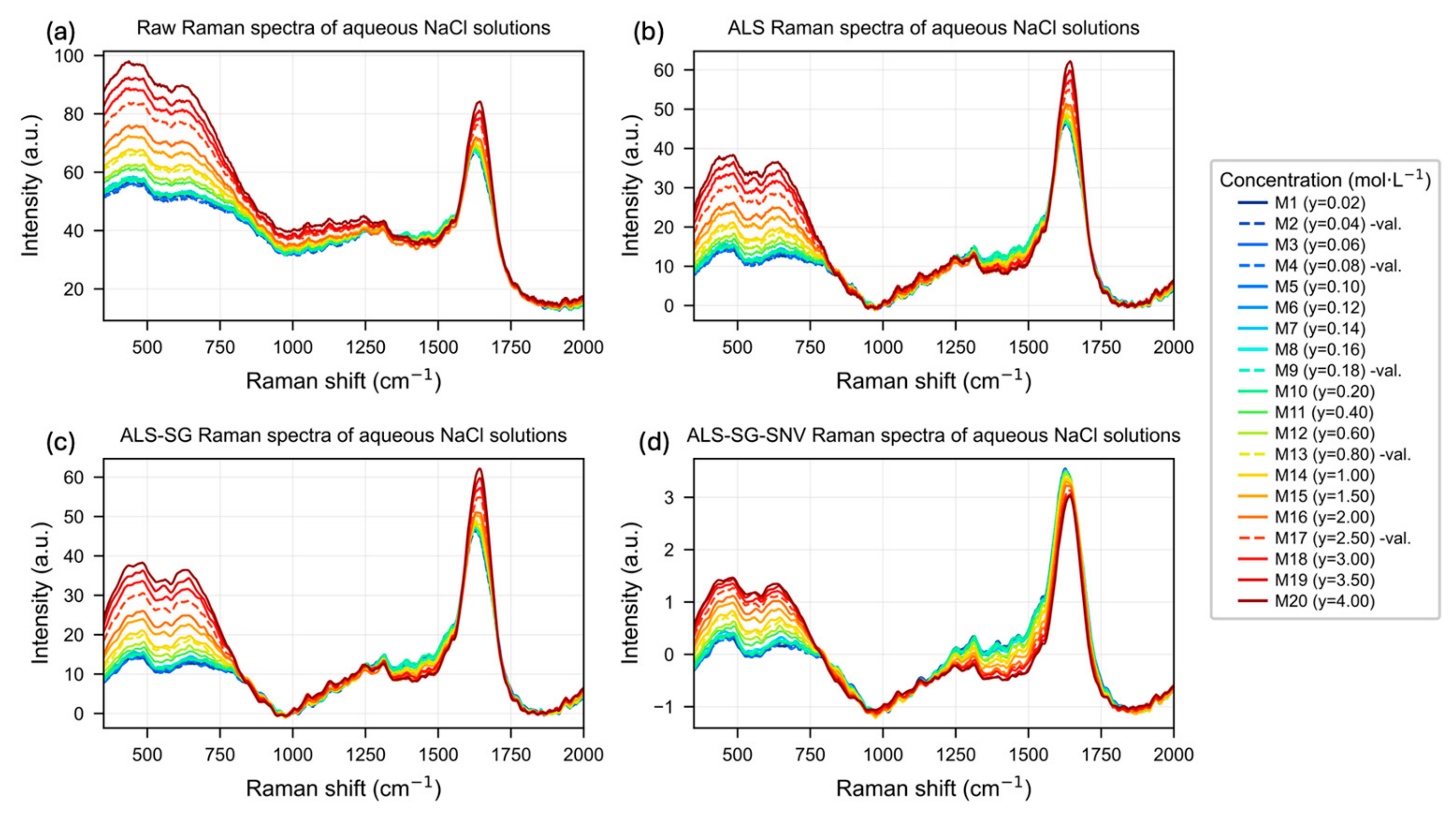
The effects of the sequential preprocessing of the Raman spectra of aqueous NaCl solutions are illustrated in Figure 2. The raw spectra (Figure 2a) exhibit a broadband background contribution that shifts the baseline proportionally to the overall intensity of each acquisition. This background introduces an intensity stepping that appears to be concentration-ordered, with the most concentrated samples (M18–M20) shifted to higher values, even in the region around 1000–1500 cm−1, where water does not exhibit active vibrational modes, thus masking the true source of the analytical variance.
Figure 2.
Raman spectra of aqueous NaCl solutions after different preprocessing steps: (a) raw spectra; (b) spectra corrected using asymmetric least squares (ALS) baseline correction; (c) spectra preprocessed by ALS followed by Savitzky–Golay filtering (ALS-SG); and (d) spectra preprocessed using ALS, Savitzky–Golay filtering, and standard normal variate normalization (ALS-SG-SNV).
However, with baseline correction using ALS (Figure 2b), signal selection is achieved in the diagnostic bands of water, namely the librational region of 450–780 cm−1 and the H-O-H bending mode at ~1640 cm−1, preserving and even enhancing the separation of spectra according to concentration, and maintaining a clear ordering of intensity from dilute to concentrated samples. In contrast, in the intermediate region of ~1000–1500 cm−1, which is spectrally uninformative, the traces are intermingled without a systematic dependence on concentration, indicating that the previous variance originated from the baseline background data rather than from an analytical response.
The subsequent application of the SG filter (ALS-SG; Figure 2c) attenuates high-frequency noise while preserving the position and profile of the bands. In contrast, normalization by SNV (ALS-SG-SNV; Figure 2d) rescales each spectrum individually and, consequently, suppresses global intensity differences linked to concentration, collapsing the spectral ensemble and eliminating precisely the quantitative information that the model aims to utilize.
3.2. PLS-R Model Calibration and Cross-Validation
The spectral behavior described above is reflected in the performance of the PLS-R models developed for each scenario (Table 2). The results require one interpretive caveat. As described in Section 2.4, the cross-validation scheme served both to compare the four preprocessing strategies and to fix the number of latent variables. This dual role is a documented source of optimistic bias, and when the same resampling scheme is used for tuning and for error estimation, the retained configuration is the one that performed best on the very partitions used to evaluate it [46]. A nested cross-validation was performed as a cautionary check and is reported below; nested or repeated cross-validation is also the appropriate approach for future work with larger calibration sets [47]. The comparison between preprocessing scenarios remains valid, since all four were evaluated under an identical partition, but the absolute values of this study should be read as internal benchmarks; the holdout set in Section 3.3 provides an additional indicator of predictive behavior, constrained by its size (n = 5). The model based on ALS-SG preprocessing yielded the lowest RMSECV (0.0608 mol·L−1), requiring only two latent variables to achieve an R2cal of 0.9990, a Q2CV of 0.9979, and an RPD of 22.54, with a negligible bias of 0.0038 mol·L−1. The model with isolated ALS correction produced virtually equivalent metrics (RMSECV = 0.0616 mol·L−1; RPD = 22.25), as well as two latent variables, confirming that baseline correction is beneficial for preserving the analytical signal for PLS modeling.
Table 2.
Comparison of calibration and cross-validation metrics for four preprocessing strategies applied prior to PLS-R model construction for NaCl quantification in aqueous solution by Raman spectroscopy (785 nm).
In contrast, raw spectra and those processed only with SG smoothing required three LVs and resulted in higher RMSECV values (0.0865 and 0.0854 mol·L−1, respectively). The inclusion of SNV markedly degraded the model, which required five latent variables and showed the poorest results of the set (RMSECV = 0.1198 mol·L−1; RPD = 11.44), consistent with the concentration-dependent loss of information, as shown in Figure 2d.
In all scenarios, the permutation test (n = 999) yielded negative mean Q2perm values and maximum values much lower than the actual Q2CV of the model, which is evidence against random correlation. Consequently, the empirical p-values were equal to 0.001 in every scenario, since no permuted model exceeded the Q2CV obtained with the correct assignment of concentrations. This value corresponds to the minimum attainable with 999 permutations under the estimator [43].
The RPD and RPIQ values follow the same ordering across the five scenarios (RPIQ: ALS-SG, 26.63; ALS, 26.29; SG, 18.96; Raw, 18.74; ALS-SG-SNV, 13.52), as expected given that both indices share the same denominator and differ only in the dispersion descriptor used in the numerator. For the present calibration, RPIQ is systematically higher than RPD by approximately 18% in every scenario; this difference reflects the shape of the concentration design. The design is deliberately asymmetric, with ten of the fifteen calibration levels below 0.20 mol·L−1 and a range spanning two orders of magnitude, so the distribution of reference values departs appreciably from normality and RPIQ was computed for this reason [40]. The magnitude of both indices is nevertheless governed by the dispersion of the calibration set, so the interpretive thresholds conventionally proposed for RPD and RPIQ, and established for calibration sets of a different structure, are not transferable to the present design. Both are therefore used here only to compare the preprocessing strategies under an identical partition.
The observed performance across the four preprocessing strategies supports the view that baseline correction is the determining preprocessing step for this system, in agreement with the importance attributed to background correction in multivariate calibration models of vibrational spectra [23]. An opposite effect was observed with SNV normalization: although the SNV transformation is used as a standard to correct multiplicative scattering variations in vibrational spectra [23,37], its application in the present system markedly degraded the model (RMSECV = 0.1198 mol·L−1, the highest; 5 LVs). This behavior can be explained by the indirect nature of the analytical signal: since quantification is based on the modulation of the absolute intensity of the water bands caused by ionic solvation, the sample-to-sample scaling inherent in SNV eliminates the concentration-dependent variance that the model requires, rather than suppressing an instrumental artifact. This result highlights that the choice of preprocessing should be consistent with the physical mechanism of signal generation, rather than based on routine application, in line with the general observation that no preprocessing technique is universally optimal and that its suitability depends on the data structure [23].
The finding that standard normal variate normalization degrades model performance carries a direct practical consequence: a calibration built on non-normalized intensities is inherently sensitive to any factor that modifies the absolute signal level, including laser output power, probe-to-sample distance, optical alignment, cuvette positioning, detector response, and sample temperature, as well as the drift accumulated between acquisition sessions [48]. In the present work, this vulnerability was minimized experimentally: all twenty solutions were measured on the same day, in a single acquisition session, on the same instrument, with identical laser power, integration time, and optical configuration. The cuvette was held in a fixed holder, and the solutions were kept in an insulated container to avoid drastic temperature changes. Under these conditions, the intensity axis can be regarded as internally consistent across the sample set, thereby allowing absolute intensity to serve as a reliable carrier of analytical information.
One possible route to address this sensitivity is intensity referencing, in which band intensities are expressed relative to an invariant reference signal, either an internal band of the solvent itself or an external standard measured under the same conditions, so that multiplicative fluctuations common to the whole spectrum are canceled [48]. In the present system, however, no truly invariant internal reference is available: the librational (450–780 cm−1) and bending bands (1640 cm−1) are not concentration-independent, since increasing NaCl content directly perturbs both modes. Their use as an internal standard would therefore suppress part of the analytical information rather than merely instrumental fluctuations. Referencing would thus require an external standard measured under identical conditions. Such a scheme was not implemented in the present study, because all spectra were acquired within a single session under fixed instrumental conditions and no inter-session correction was needed. Its incorporation, along with an evaluation of prediction performance across independent acquisition sessions, constitutes a necessary step whenever the acquisition conditions described above cannot be kept invariant.
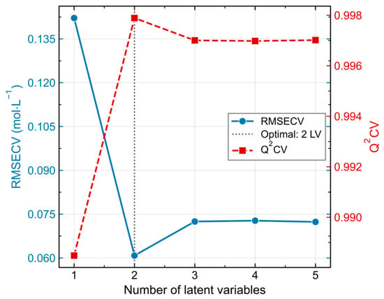
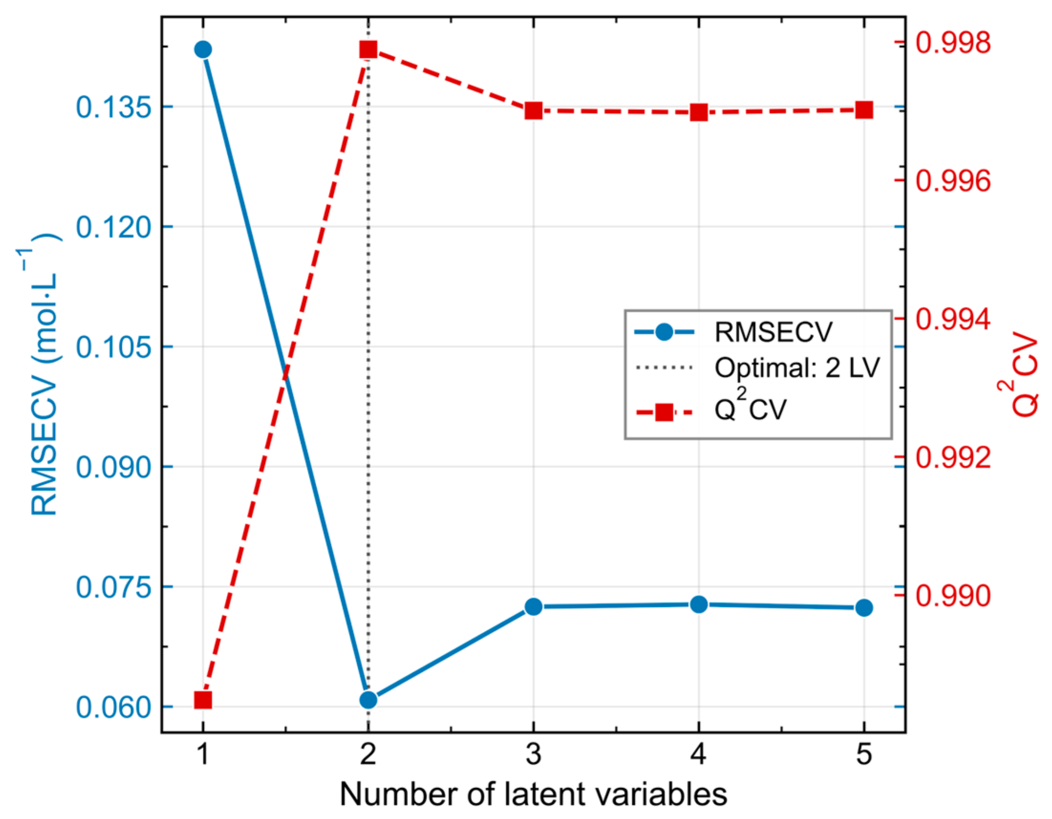
In addition, the evolution of RMSECV and Q2CV as a function of the number of LVs for the ALS–SG-preprocessed PLS-R model, evaluated by Venetian blinds cross-validation (k = 3), is shown in Figure 3. RMSECV decreased sharply from a high value with a single latent variable to a minimum of 0.0608 mol·L−1 with two latent variables, at which point Q2CV simultaneously reached its maximum (0.9979). The inclusion of additional components did not produce improvements in predictive capacity: RMSECV stabilized slightly above the minimum and Q2CV remained essentially constant. Therefore, the two-latent-variable model was selected, based on the principle of parsimony, thus avoiding overfitting.
Figure 3.
Selection of the optimal number of LVs for the PLS-R model using Venetian blinds cross-validation (k = 3). The left y-axis (blue, solid line) shows the RMSECV (mol·L−1), and the right y-axis (red, dashed line) shows the Q2CV, both plotted as a function of the number of PLS-R components. The vertical dotted line indicates the selected model (2 LVs), corresponding to the minimum RMSECV (0.0608 mol·L−1) and the maximum Q2CV (0.9979), beyond which no significant improvement in predictive performance was observed.
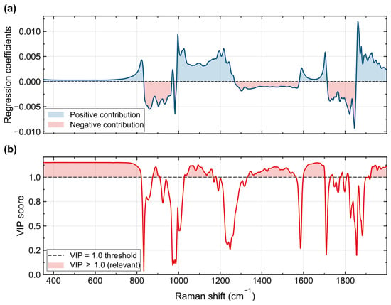
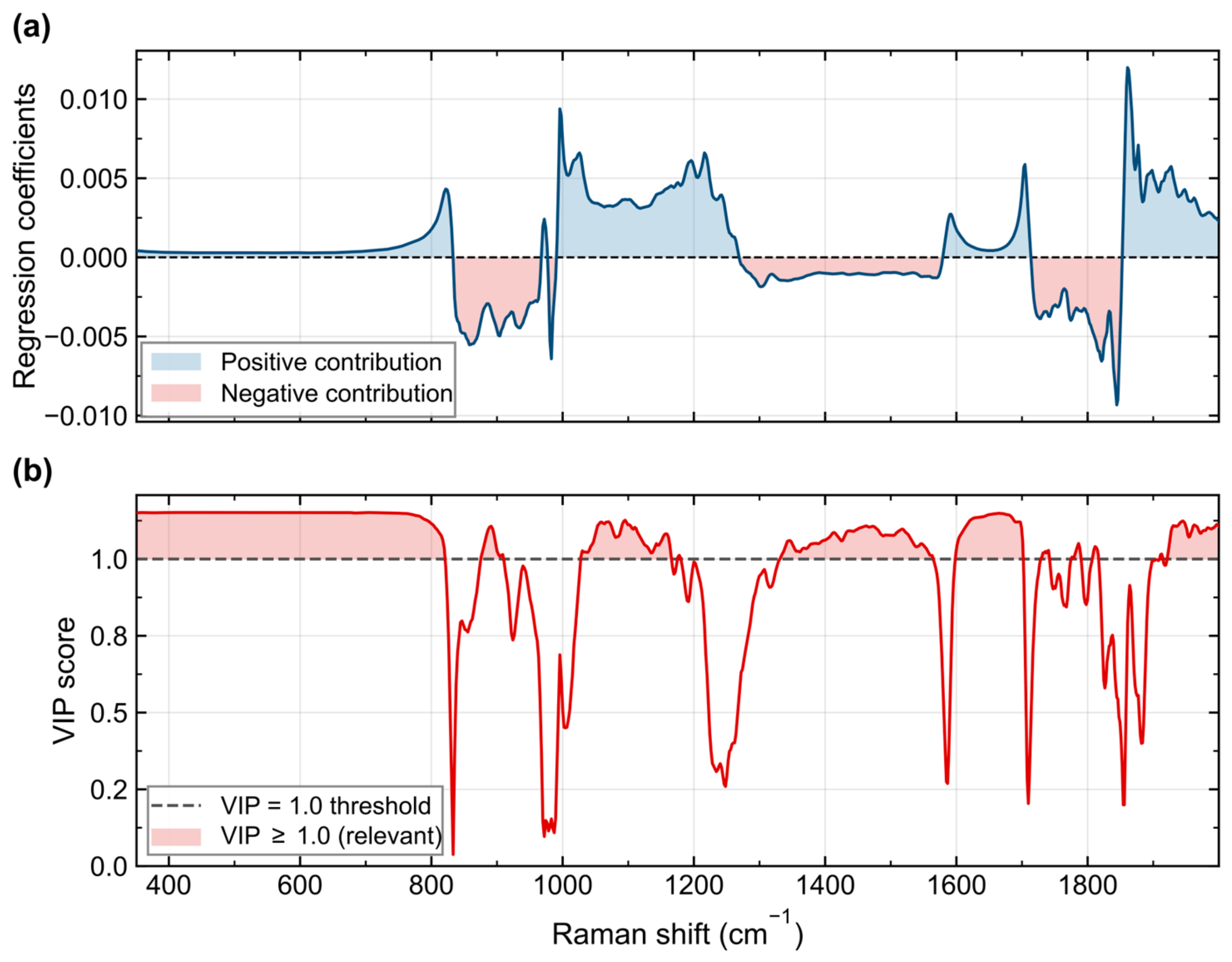
Analysis of the regression coefficients (Figure 4a) and VIP values (Figure 4b) of the selected model indicates that the variables with VIP ≥ 1.0, a threshold that, by interpretive convention, identifies variables regarded as influential for the calibration model, are concentrated in two spectral regions: the H-O-H bending band of water (~1640 cm−1) and the low-frequency librational mode region (~450–780 cm−1). These exhibit the highest VIP values. It is worth noting, however, that the VIP profile does not consist of sharp, isolated peaks. Instead, the variables with VIP ≥ 1.0 are distributed in broad, continuous bands with values that barely exceed this threshold (maximums around 1.1–1.2). This pattern is consistent with the physical mechanism for detecting NaCl in solution using Raman spectroscopy, and the spectral relevance is distributed over extensive regions associated with the solvent structure, rather than being concentrated in discrete spectral features. The profile of the regression coefficients, characterized by alternating positive and negative contributions across the spectrum, further confirms that the model integrates this distributed information in a multivariate manner, capturing subtle changes across multiple diagnostic regions rather than relying on a single spectral feature.
Figure 4.
Spectral relevance of the PLS-R model (2 LVs, ALS–SG preprocessing). (a) Regression coefficients as a function of Raman shift; blue regions indicate positive contributions to concentration prediction, whereas red regions indicate negative contributions. (b) Variable importance in projection (VIP) scores as a function of Raman shift. The dashed gray line denotes the VIP = 1.0 threshold, above which variables are considered relevant for prediction [41]. Red-shaded regions correspond to variables with VIP ≥ 1.0. The H-O-H bending mode of water (~1640 cm−1) and the librational region (~450–780 cm−1) exhibit the highest VIP values, consistent with the perturbation of the water hydrogen-bond network induced by Na+ and Cl− ions.
The distribution of analytical information across broad spectral regions provides insight into the physicochemical mechanisms responsible for the observed response. Na+ and Cl− ions are monatomic species that lack Raman-active vibrational modes. Therefore, the quantitative signal does not originate from solute bands themselves, but rather from the perturbation that ion solvation induces on the hydrogen-bond network of water, manifested as variations in the librational modes [44] and the H-O-H bending of the solvent [44,45]. As NaCl dissolves, an increasing fraction of water molecules is recruited into the hydration shells of Na+ and Cl−, where their orientation and hydrogen bonding differ from those of bulk water; the proportion of water participating in the extended tetrahedral network consequently decreases with concentration, and both spectral regions change accordingly. The fact that the model prioritizes broad spectral regions over discrete signals is a characteristic feature of the indirect detection mechanism and justifies the application of multivariate approaches instead of the univariate band-ratio-based analysis used in previous Raman studies of NaCl solutions [13,14]. While such univariate approaches rely on intensities measured at discrete spectral positions, the simultaneous extraction of information from multiple diagnostic regions is expected to confer greater stability to the prediction, in line with the application of chemometrics to the study of water structure by vibrational spectroscopy, where the analytical signal is also based on indirect structural perturbations of the solvent [24].
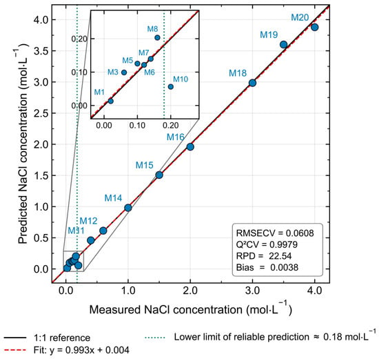
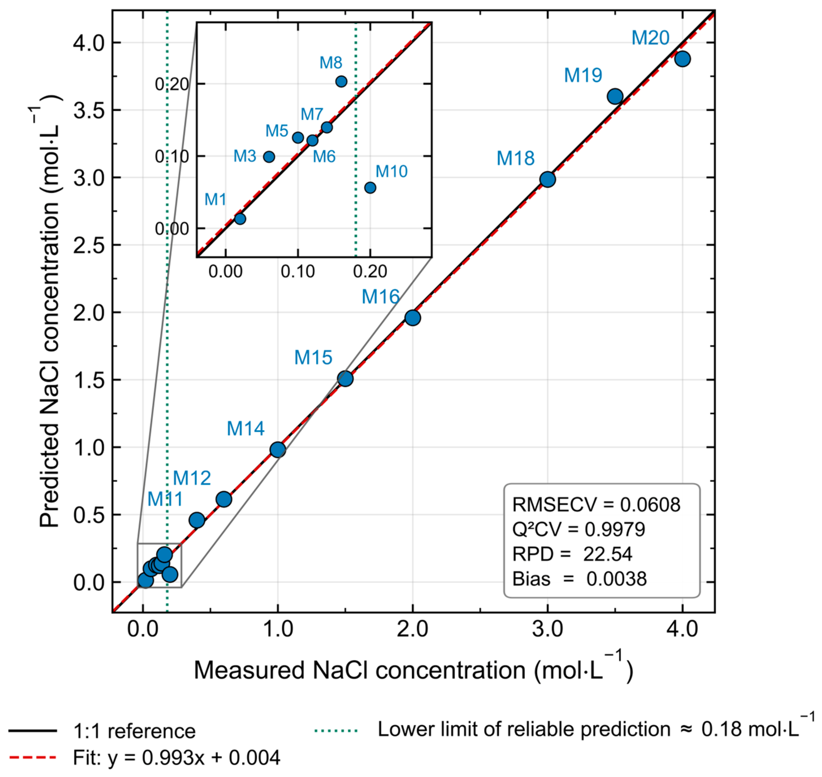
Based on the selected model (ALS-SG, 2 LVs), evaluated using cross-validation with Venetian blinds on the fifteen samples of the calibration set, the predicted concentrations were compared against the reference concentrations (Figure 5). The results show a distribution fitted to the 1:1 identity line across the calibration range (0.02 to 4.0 mol·L−1), with a regression line practically coinciding with the ideal relationship (y = 0.993x + 0.004). The calibration metrics (Table 2) indicate close agreement with the reference values across the calibration range. The higher density of levels in the lower subrange (M1–M10, ≤0.20 mol·L−1) corresponds to the experimental design, in which this subrange was anticipated to represent the most challenging region for model performance because the weak perturbation of the water structure induced by ionic solvation makes quantification more difficult. Therefore, sampling was reinforced in this subrange to provide the model with additional calibration data where the analytical response is weaker and thus define more accurately the empirical lower limit of reliable prediction.
Figure 5.
Predicted versus measured NaCl concentrations for the PLS-R calibration model developed from Raman spectra preprocessed with ALS baseline correction and an SG filter, evaluated using cross-validation of Venetian blinds (k = 3). The solid black line indicates the ideal 1:1 relationship, while the dashed red line represents the least-squares regression between predicted and measured concentrations. Each marker corresponds to an individual calibration sample identified by its sample code. The inset shows the model performance metrics (R2cal, RMSECV, Q2CV, RPD, and bias).
Finally, as an additional procedure to provide more information on the optimistic metrics, nested cross-validation was performed using the same Venetian blinds scheme in both loops. The outer loop partitions the 15 calibration samples into k = 3 interleaved segments in the same manner as described above. Within each outer training partition, an inner Venetian blinds loop (k = 3) selects the number of latent variables by minimizing the inner RMSECV over the number of LVs (1–5). A PLS-R model with the selected complexity is then fitted on the full outer training partition and used to predict the corresponding outer test partition. Because each outer test sample is excluded from both the inner selection loop and the outer fit, the nested RMSECV and Q2CV are free of the selection-induced optimistic bias described by Varma and Simon [46] and Krstajic et al. [47]. The results of this procedure were nested RMSECV = 0.0778 mol·L−1, nested Q2CV = 0.9965, and nested bias = 0.0076 mol·L−1. However, across the three outer folds, the inner loop selected a different complexity in each case (2, 3, and 5 LVs), and the corresponding inner RMSECV values differed notably (0.0874, 0.0989, and 0.0653 mol·L−1). The disagreement between the outer folds, together with the increasing complexity, indicates that the inner selection criterion did not converge to a single model due to the small training partitions (10 samples, with 6 or 7 samples in each inner training split). Consequently, nested cross-validation in this work should be regarded as a cautionary check, and, as mentioned above, nested or repeated cross-validation is the appropriate approach for future work with larger calibration sets.
3.3. Holdout Prediction Performance
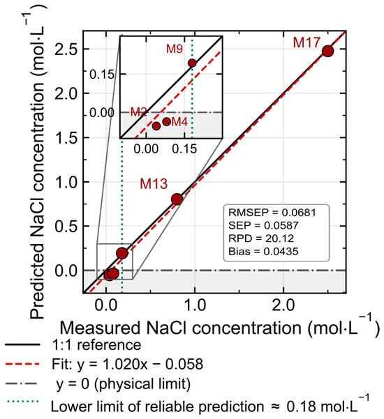
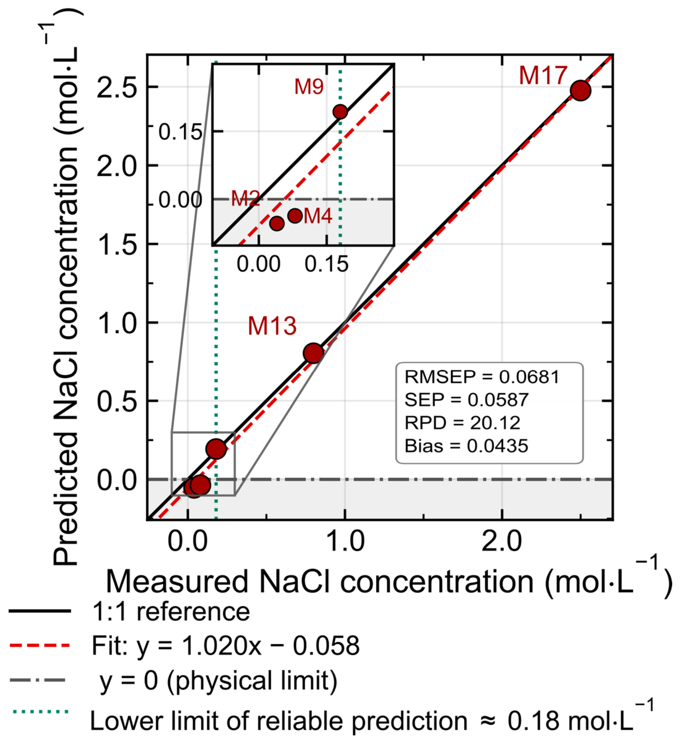
The results of the evaluated model on the holdout prediction set (M2, M4, M9, M13, and M17) are presented in Figure 6 and Table 3. The model achieved an R2ext of 0.9946, an RMSEP of 0.0681 mol·L−1, an SEP of 0.0587 mol·L−1, and a holdout RPD of 20.12, with a bias of 0.0435 mol·L−1. The intermediate- and high-concentration samples were predicted with absolute relative errors below 8%: the absolute relative errors for M9 (−0.013 mol·L−1), M13 (−0.005 mol·L−1), and M17 (0.024 mol·L−1) were 7.24%, 0.56%, and 0.97%, respectively. In contrast, the two lowest-concentration samples produced predictions outside the physical range (negative concentrations: −0.054 mol·L−1 for M2 and −0.037 mol·L−1 for M4), with prediction errors of 0.094 and 0.117 mol·L−1. This behavior indicates that both samples fall below the empirical lower limit of reliable prediction of the model (~0.18 mol·L−1), where the perturbation induced on the water structure is too weak to be distinguished from residual noise and baseline variability. For these two samples the relative errors listed in Table 3 (234.56% and 146.01%) are not meaningful performance indicators, since they merely express a prediction of the wrong sign; they are reported for completeness only. The model therefore behaves in two clearly distinct regimes, and the global R2ext and RMSEP of the holdout set, being dominated by the two highest-concentration samples, do not describe performance across the whole range. Given the small size of the holdout set, the R2ext value should be interpreted with caution [38]; however, the metrics obtained are consistent with quantification from approximately 0.18 mol·L−1 upward, although this indication rests on only three holdout samples and the highest of them corresponds to 2.50 mol·L−1. The interval between 2.50 and 4.00 mol·L−1 is therefore supported by calibration and cross-validation only.
Figure 6.
Predicted versus reference NaCl concentrations for the holdout prediction set (n = 5; samples M2, M4, M9, M13, and M17). The PLS-R model was built using two latent variables and spectra preprocessed by ALS baseline correction followed by SG smoothing. The solid black line represents the ideal 1:1 relationship, and the dashed red line represents the linear regression of the predicted values. Model performance metrics were as follows: coefficient of determination, R2ext = 0.9946; root mean square error of prediction, RMSEP = 0.0681 mol·L−1; standard error of prediction, SEP = 0.0587 mol·L−1; RPDext = 20.12 (calculated according to Bellon-Maurel et al. [40]); and holdout bias = 0.0435 mol·L−1. The interpretation of these metrics should be made with caution because of the limited size of the holdout set.
Table 3.
Prediction errors for the samples included in the holdout prediction set using the selected PLS-R model (ALS–SG preprocessing, 2 LVs).
Using the criterion of Bellon-Maurel et al. [40] as a guide, according to which values above 2.0 are considered indicative of adequate predictive capacity, the obtained holdout RPD of 20.12 suggests the potential suitability of the model for quantifying NaCl over the interval actually covered by the holdout samples (0.18–2.50 mol·L−1), with the limitation already noted regarding the size of the holdout set (n = 5). Nevertheless, RPD is best interpreted as a relative performance index rather than an absolute measure of accuracy across the working range; as RPD is the ratio between the dispersion of a set of reference concentrations and a single global error term, it grows without bound as the calibration range is widened at constant RMSEP.
The empirical lower limit of reliable prediction lies below the salinity levels of seawater (0.54 mol·L−1 on average), the brines used in food processing (0.34–3.42 mol·L−1) [2], and those employed in the chlor-alkali industry (0.34–5.44 mol·L−1) [5], all of which fall within the calibration range explored here. It lies, however, above the concentration of isotonic saline solutions (0.154 mol·L−1) and well above the residual salinity of desalinated product water, which are consequently outside the range in which the model was assessed. This threshold should be read as a guide to the applications worth exploring in future work rather than as a demonstration of applicability, since none of these matrices was examined here. On the basis of the present calibration, the approach appears better suited to the monitoring of concentrated streams than to the analysis of dilute ones, although extending it to the low-concentration region through a dedicated acquisition and calibration design, specifically populated in that range, remains an open possibility.
3.4. Strengths and Limitations of the PLS-R Approach
Previous Raman determinations of NaCl (Table 1) read the perturbation induced by ion hydration from the O–H stretching band; the model developed here was built on the 350–2000 cm−1 region alone, and the VIP analysis (Figure 4b) assigned the highest values to the librational and H–O–H bending regions. Within the conditions tested, these results indicate that this region carries sufficient information for NaCl quantification with a two-latent-variable model, which is relevant for 785 nm configurations in which the O–H stretching band cannot be recorded. The treatment of that information also differs from the univariate band-ratio analyses applied in earlier Raman studies of NaCl solutions [13]: rather than intensities measured at two discrete spectral positions, the model integrates information distributed across the librational and H–O–H bending envelopes, which in principle should confer greater tolerance to baseline variations than a ratio between two discrete bands. A band-ratio does not compensate for residual additive contributions, which propagate unequally to the numerator and denominator. A multivariate treatment is, in principle, less affected by this phenomenon, because in PLS-R, such contributions occupy a low-dimensional subspace that is largely separable from the direction along which concentration information is extracted, provided that the corresponding variability is represented in the calibration set. This is the general argument for multivariate over univariate calibration when interfering contributions cannot be resolved at a single spectral position [49]. As noted above, a band-ratio approach retains an intrinsic advantage against purely multiplicative fluctuations, such as variations in laser power, but it could not be adopted here because no concentration-invariant internal reference band exists in this system.
Compared with methods based on near-infrared spectroscopy coupled with PLS-R, which constitute the most widespread instrumental alternative for the determination of salts in aqueous solution [31,32,33,34], the results of this proof-of-concept study suggest that a Raman approach may achieve comparable accuracy while relying on a more parsimonious model with a small number of latent variables, and its implementation therefore merits further exploration. The reduced complexity of the model, with just two components, is consistent with the observation that near-infrared calibrations, by relying on wider and overlapping combination bands and overtones, tend to require a greater number of latent variables [31,32,33,34], and reinforces interest in Raman spectroscopy as a complementary technique for monitoring processes in aqueous media. Nonetheless, the empirical lower limit of reliable prediction (~0.18 mol·L−1) suggests that the main limiting factor of the method is imposed by the weak perturbation that low concentrations of NaCl exert on the water structure.
The analytical signal exploited here originates in the perturbation that ion solvation exerts on the hydrogen-bond network of water and is therefore not specific to the identity of the dissolved ions. Different electrolytes modify water structure in different directions and to different extents [50], so the present calibration cannot separate the individual contributions of cations and anions, nor distinguish between the effects of ion identity, ion concentration and total ionic strength. Since all calibration and holdout samples were prepared from analytical-grade NaCl in distilled water and originated from the same batch and acquisition session, the interference of coexisting ions such as K+, Mg2+ and Ca2+ was not evaluated, and no conclusion can be drawn regarding additive, antagonistic or nonlinear behavior in mixed electrolyte systems.
The present work establishes only the feasibility of the PLS-R approach on a simple, controlled NaCl matrix and delimits the conditions under which it may be developed further for monitoring aqueous media. A larger number of calibration samples and an independent validation set (including measurements on different days and under varied instrumental conditions) are necessary to generalize the model even within a simple matrix, while its extrapolation to multicomponent matrices, along with selectivity and interference studies and validation on real samples, requires an independent experimental design and constitutes the next stage in the development of this methodology.
4. Conclusions
Unlike previous Raman determinations of NaCl, which read the perturbation induced by ion hydration from the O–H stretching band, this study shows that the librational (450–780 cm−1) and H–O–H bending (~1640 cm−1) regions alone carry sufficient information for PLS-R quantification of NaCl in simple, controlled aqueous solutions. This is directly relevant to 785 nm fiber-probe configurations, in which the O–H stretching band lies beyond the detection window of silicon CCD detectors.
Quantification was demonstrated on holdout samples between approximately 0.18 and 2.50 mol·L−1, while the calibration model extends to 4.0 mol·L−1. The optimal model, based on a combination of ALS and SG smoothing, required only two LVs and was assessed by cross-validation, permutation tests, and a holdout prediction set. The results demonstrate that spectral preprocessing should be selected according to the physical mechanism of Raman signal formation. Baseline correction was beneficial for model performance, while SNV normalization eliminated some analytical information by reducing intensity variations associated with concentration. Furthermore, the distribution of VIP values supported the interpretation that NaCl quantification is based on the perturbation that ionic solvation exerts on the water structure, supporting the use of multivariate strategies over univariate approaches. The empirical lower limit of reliable prediction (~0.18 mol·L−1) precludes the application of the method to very diluted solutions, and the holdout set should be expanded with a larger number of independently prepared samples distributed across the low-, intermediate- and high-concentration regions. Within these constraints, the study is presented as a proof of concept: it establishes the feasibility of the approach on a simple, controlled NaCl matrix and delimits the conditions under which it may be developed further for monitoring aqueous media.
Author Contributions
J.A.P.-M.: conceptualization, methodology, investigation, formal analysis, software, data curation, visualization, writing—original draft, funding acquisition. A.F.G. and S.M.-V.: methodology, investigation, validation, resources. J.G.F.T. and O.B.: investigation, formal analysis, writing—review and editing. L.D.l.C.M.: writing—review and editing, supervision, project administration. M.E.-R.: conceptualization, methodology, formal analysis, data curation, writing—review and editing, supervision, project administration. All authors have read and agreed to the published version of the manuscript.
Funding
This research received no external funding.
Data Availability Statement
The data presented in this study are openly available in Zenodo at https://doi.org/10.5281/zenodo.21780426.
Conflicts of Interest
The authors declare no conflicts of interest. The funders had no role in the design of the study; in the collection, analyses, or interpretation of the data; in the writing of the manuscript; or in the decision to publish the results.
Abbreviations
The following abbreviations are used in this manuscript:
| NaCl | Sodium chloride |
| PLS-R | Partial least squares regression |
| ALS-SG | Asymmetric least squares baseline correction and Savitzky–Golay smoothing |
| R2cal | Calibration coefficient of determination |
| Q2CV | Cross-validated coefficient of determination |
| RMSECV | Root mean square error of cross-validation |
| R2ext | Holdout coefficient of determination |
| RMSEP | Root mean square error of prediction |
| SG | Savitzky–Golay |
| ALS | Asymmetric least squares |
| FFT-CCD | Full-frame transfer charge-coupled device |
| SNV | Standard normal variate |
| SNR | Signal-to-noise ratio |
| NIPALS | Nonlinear iterative partial least squares algorithm |
| LVs | Latent variables |
| RPD | Residual predictive deviation |
| SDcal | Standard deviation of calibration |
| RPIQ | Ratio of performance to interquartile distance |
| VIP | Variable importance in projection |
| Q2 | Coefficient of determination |
| Q2perm | Permuted coefficient of determination |
| SEP | Standard error of prediction |
References
- Taormina, P.J. Implications of salt and sodium reduction on microbial food safety. Crit. Rev. Food Sci. Nutr. 2010, 50, 209–227. [Google Scholar] [CrossRef] [Scilit] [PubMed]
- Khan, A.W.; Roobab, U.; Wang, Z.; Raza, M.M.; Nawazish, H.; Islam, F.; Aadil, R.M. Salt reduction in food products: A systematic review of clean-label ingredients and non-thermal technologies. Trends Food Sci. Technol. 2024, 153, 104695. [Google Scholar] [CrossRef] [Scilit]
- Ruusunen, M.; Puolanne, E. Reducing sodium intake from meat products. Meat Sci. 2005, 70, 531–541. [Google Scholar] [CrossRef] [Scilit] [PubMed]
- Wang, J.; Huang, X.H.; Zhang, Y.Y.; Li, S.; Dong, X.; Qin, L. Effect of sodium salt on meat products and reduction sodium strategies—A review. Meat Sci. 2023, 205, 109296. [Google Scholar] [CrossRef] [Scilit] [PubMed]
- O’Brien, T.F.; Bommaraju, T.V.; Hine, F. Handbook of Chlor-Alkali Technology: Volume I–V; Springer: New York, NY, USA, 2005. [Google Scholar]
- World Health Organization (WHO). Guidelines for Drinking-Water Quality, 4th ed.; WHO Press: Geneva, Switzerland, 2022. [Google Scholar]
- Cai, L.; Ouyang, Z.; Song, J.; Yang, L. Indicator-free argentometric titration for distance-based detection of chloride using microfluidic paper-based analytical devices. ACS Omega 2020, 5, 18935–18940. [Google Scholar] [CrossRef] [Scilit] [PubMed]
- Feng, R.; Lin, X. RFID-based real-time salt concentration monitoring with adaptive EKF. Sensors 2025, 25, 3826. [Google Scholar] [CrossRef] [Scilit] [PubMed]
- Lide, D.R. (Ed.) CRC Handbook of Chemistry and Physics, 84th ed.; CRC Press: Boca Raton, FL, USA, 2003. [Google Scholar]
- McCreery, R.L. Raman Spectroscopy for Chemical Analysis; Wiley-Interscience: New York, NY, USA, 2000. [Google Scholar]
- Strachan, C.J.; Rades, T.; Gordon, K.C.; Rantanen, J. Raman spectroscopy for quantitative analysis of pharmaceutical solids. J. Pharm. Pharmacol. 2007, 59, 179–192. [Google Scholar] [CrossRef] [Scilit] [PubMed]
- Ferraro, J.R.; Nakamoto, K.; Brown, C.W. Introductory Raman Spectroscopy, 2nd ed.; Academic Press: San Diego, CA, USA, 2003. [Google Scholar]
- Đuričković, I.; Marchetti, M.; Claverie, R.; Bourson, P.; Chassot, J.M.; Fontana, M.D. Experimental study of NaCl aqueous solutions by Raman spectroscopy: Towards a new optical sensor. Appl. Spectrosc. 2010, 64, 853–857. [Google Scholar] [CrossRef] [Scilit] [PubMed]
- Claverie, R.; Fontana, M.D.; Đuričković, I.; Bourson, P.; Marchetti, M.; Chassot, J.M. Optical sensor for characterizing the phase transition in salted solutions. Sensors 2010, 10, 3815–3823. [Google Scholar] [CrossRef] [Scilit] [PubMed]
- Geladi, P.; Kowalski, B.R. Partial least-squares regression: A tutorial. Anal. Chim. Acta 1986, 185, 1–17. [Google Scholar] [CrossRef] [Scilit]
- Wold, S.; Sjöström, M.; Eriksson, L. PLS-regression: A basic tool of chemometrics. Chemom. Intell. Lab. Syst. 2001, 58, 109–130. [Google Scholar] [CrossRef] [Scilit]
- Martens, H.; Næs, T. Multivariate Calibration; Wiley: New York, NY, USA, 1992. [Google Scholar]
- Elderderi, S.; Wils, L.; Leman-Loubière, C.; Henry, S.; Byrne, H.J.; Chourpa, I.; Munnier, E.; Elbashir, A.A.; Boudesocque-Delaye, L.; Bonnier, F. Comparison of Raman and attenuated total reflectance (ATR) infrared spectroscopy for water quantification in natural deep eutectic solvent. Anal. Bioanal. Chem. 2021, 413, 4785–4799. [Google Scholar] [CrossRef] [Scilit] [PubMed]
- Zhao, M.; Shaikh, S.; Kang, R.; Markiewicz-Keszycka, M. Investigation of Raman spectroscopy (with fiber optic probe) and chemometric data analysis for the determination of mineral content in aqueous infant formula. Foods 2020, 9, 968. [Google Scholar] [CrossRef] [Scilit] [PubMed]
- Rubini, M.; Boyer, J.; Poulain, J.; Berger, A.; Saillard, T.; Louet, J.; Soucé, M.; Roussel, S.; Arnould, S.; Vergès, M.; et al. Monitoring of nutrients, metabolites, IgG titer, and cell densities in 10 L bioreactors using Raman spectroscopy and PLS regression models. Pharmaceutics 2025, 17, 473. [Google Scholar] [CrossRef] [Scilit] [PubMed]
- Savitzky, A.; Golay, M.J.E. Smoothing and differentiation of data by simplified least squares procedures. Anal. Chem. 1964, 36, 1627–1639. [Google Scholar] [CrossRef] [Scilit]
- Eilers, P.H.C. A perfect smoother. Anal. Chem. 2003, 75, 3631–3636. [Google Scholar] [CrossRef] [Scilit] [PubMed]
- Rinnan, Å.; van den Berg, F.; Engelsen, S.B. Review of the most common pre-processing techniques for near-infrared spectra. TrAC. Trends Anal. Chem. 2009, 28, 1201–1222. [Google Scholar] [CrossRef] [Scilit]
- Wang, H.; Han, L.; Cai, W.; Shao, X. Chemometrics: A vital implement for understanding the water structures by near-infrared spectroscopy. J. Chemom. 2024, 38, e3631. [Google Scholar] [CrossRef] [Scilit]
- Furić, K.; Ciglenečki, I.; Ćosović, B. Raman spectroscopic study of sodium chloride water solutions. J. Mol. Struct. 2000, 550–551, 225–234. [Google Scholar] [CrossRef] [Scilit]
- Sun, Q.; Zhao, L.; Li, N.; Liu, J. Raman spectroscopic study for the determination of Cl− concentration (molarity scale) in aqueous solutions: Application to fluid inclusions. Chem. Geol. 2010, 272, 55–61. [Google Scholar] [CrossRef] [Scilit]
- He, X.; Wang, W.-Q.; Liu, Y.-Z.; Sun, Q. Raman quantitative measurement on the Cl− molarity of H2O-NaCl-CO2 system: Application to fluid inclusions. Minerals 2024, 14, 1121. [Google Scholar] [CrossRef] [Scilit]
- Burikov, S.A.; Dolenko, T.A.; Fadeev, V.V.; Sugonyaev, A.V. Identification of inorganic salts and determination of their concentrations in aqueous solutions based on the valence Raman band of water using artificial neural networks. Pattern Recognit. Image Anal. 2007, 17, 554–559. [Google Scholar] [CrossRef] [Scilit]
- Efitorov, A.O.; Burikov, S.A.; Dolenko, T.A.; Persiantsev, I.G.; Dolenko, S.A. Comparison of the quality of solving the inverse problems of spectroscopy of multi-component solutions with neural network methods and with the method of projection to latent structures. Opt. Mem. Neural Netw. 2015, 24, 93–101. [Google Scholar] [CrossRef] [Scilit]
- Pérez, E.; Sbárbaro, D.; Fuentes, R.; Castillo, F. Estimation of NaCl Concentration in Aqueous Solution Using Partial Least Square Regression and Raman Spectroscopy. In Proceedings of the 2025 IEEE Chilean Conference on Electrical, Electronics Engineering, Information and Communication Technologies (CHILECON), Valparaíso, Chile, 28–30 October 2025. [Google Scholar] [CrossRef] [Scilit]
- Lin, J.; Brown, C.W. Near-IR spectroscopic determination of NaCl in aqueous solution. Appl. Spectrosc. 1992, 46, 1809–1815. [Google Scholar] [CrossRef] [Scilit]
- Gowen, A.A.; Marini, F.; Tsuchisaka, Y.; De Luca, S.; Bevilacqua, M.; O’Donnell, C.; Downey, G.; Tsenkova, R. On the feasibility of near infrared spectroscopy to detect contaminants in water using single salt solutions as model systems. Talanta 2015, 131, 609–618. [Google Scholar] [CrossRef] [Scilit] [PubMed]
- Wu, R.; Xue, J.; Tian, H.; Dong, C. Qualitative discrimination and quantitative prediction of salt in aqueous solution based on near-infrared spectroscopy. Talanta 2025, 281, 126751. [Google Scholar] [CrossRef] [Scilit] [PubMed]
- Peters, R.D.; Noble, S.D. Using near infrared measurements to evaluate NaCl and KCl in water. J. Near Infrared Spectrosc. 2019, 27, 147–155. [Google Scholar] [CrossRef] [Scilit] [PubMed]
- Zhang, Z.-M.; Chen, S.; Liang, Y.-Z. Baseline correction using adaptive iteratively reweighted penalized least squares. Analyst 2010, 135, 1138–1146. [Google Scholar] [CrossRef] [Scilit] [PubMed]
- Vivó-Truyols, G.; Schoenmakers, P.J. Automatic selection of optimal Savitzky–Golay smoothing. Anal. Chem. 2006, 78, 4598–4608. [Google Scholar] [CrossRef] [Scilit] [PubMed]
- Barnes, R.J.; Dhanoa, M.S.; Lister, S.J. Standard normal variate transformation and de-trending of near-infrared diffuse reflectance spectra. Appl. Spectrosc. 1989, 43, 772–777. [Google Scholar] [CrossRef] [Scilit]
- Westad, F.; Marini, F. Validation of chemometric models—A tutorial. Anal. Chim. Acta 2015, 893, 14–24. [Google Scholar] [CrossRef] [Scilit] [PubMed]
- Ezenarro, J.; Schorn-García, D. How Are Chemometric Models Validated? A Systematic Review of Linear Regression Models for NIRS Data in Food Analysis. J. Chemom. 2025, 39, e70036. [Google Scholar] [CrossRef] [Scilit]
- Bellon-Maurel, V.; Fernandez-Ahumada, E.; Palagos, B.; Roger, J.-M.; McBratney, A. Critical review of chemometric indicators commonly used for assessing the quality of the prediction of soil attributes by NIR spectroscopy. TrAC Trends Anal. Chem. 2010, 29, 1073–1081. [Google Scholar] [CrossRef] [Scilit]
- Chong, I.-G.; Jun, C.-H. Performance of some variable selection methods when multicollinearity is present. Chemom. Intell. Lab. Syst. 2005, 78, 103–112. [Google Scholar] [CrossRef] [Scilit]
- Lindgren, F.; Hansen, B.; Karcher, W.; Sjöström, M.; Eriksson, L. Model validation by permutation tests: Applications to variable selection. J. Chemom. 1996, 10, 521–532. [Google Scholar] [CrossRef]
- Phipson, B.; Smyth, G.K. Permutation P-values should never be zero: Calculating exact P-values when permutations are randomly drawn. Stat. Appl. Genet. Mol. Biol. 2010, 9, 1–12. [Google Scholar] [CrossRef] [Scilit] [PubMed]
- Walrafen, G.E. Raman spectral studies of water structure. J. Chem. Phys. 1964, 40, 3249–3256. [Google Scholar] [CrossRef] [Scilit]
- Sun, Q.; Qin, C. Raman OH stretching band of water as an internal standard to determine carbonate concentrations. Chem. Geol. 2011, 283, 274–278. [Google Scholar] [CrossRef] [Scilit]
- Varma, S.; Simon, R. Bias in error estimation when using cross-validation for model selection. BMC Bioinform. 2006, 7, 91. [Google Scholar] [CrossRef] [Scilit] [PubMed]
- Krstajic, D.; Buturovic, L.J.; Leahy, D.E.; Thomas, S. Cross-validation pitfalls when selecting and assessing regression and classification models. J. Cheminform. 2014, 6, 10. [Google Scholar] [CrossRef] [Scilit] [PubMed]
- Pelletier, M.J. Quantitative analysis using Raman spectrometry. Appl. Spectrosc. 2003, 57, 20A–42A. [Google Scholar] [CrossRef] [Scilit] [PubMed]
- Guizani, C.; Hellstén, S.; Witos, J.; Sixta, H. Quantitative Raman spectroscopy for the Ioncell™ process. Part 1: Comparison of univariate and multivariate calibration methods for the quantification of water and protic ionic liquid components. Cellulose 2020, 27, 157–170. [Google Scholar] [CrossRef] [Scilit]
- Ahmed, M.; Namboodiri, V.; Singh, A.K.; Mondal, J.A. On the intermolecular vibrational coupling, hydrogen bonding, and librational freedom of water in the hydration shell of mono- and bivalent anions. J. Chem. Physics. 2014, 141, 164708. [Google Scholar] [CrossRef] [Scilit] [PubMed]

Disclaimer/Publisher’s Note: The statements, opinions and data contained in all publications are solely those of the individual author(s) and contributor(s) and not of MDPI and/or the editor(s). MDPI and/or the editor(s) disclaim responsibility for any injury to people or property resulting from any ideas, methods, instructions or products referred to in the content. |
© 2026 by the authors. Licensee MDPI, Basel, Switzerland. This article is an open access article distributed under the terms and conditions of the Creative Commons Attribution (CC BY) license.