


Abstract
Mangrove-fringed coastal areas provide habitat and sediment regulation ecosystem services, increasingly affected by land-use change. However, integrated local-scale assessments of habitat quality and sediment dynamics remain limited. This study assessed land-use and land-cover (LULC) changes in Mueang Samut Sakhon District, Thailand, for 2000–2020 and projected a business-as-usual (BAU) scenario for 2040 using a cellular automata-artificial neural network model (hindcast overall accuracy 74.7%). Habitat quality and sediment dynamics were assessed for 2000, 2020, and 2040 using the InVEST Habitat Quality and Sediment Delivery Ratio models, and tested with an independent mangrove dataset, sensitivity analyses, and an analysis by LULC transition. Between 2000 and 2020, built-up land increased by 34.7% and mapped mangroves declined by 50.6%, with further changes of +4.8% and −9.3% projected for 2040. Global Mangrove Watch indicated a smaller decline (29%), so the mapped loss is an upper estimate. Total habitat quality declined by 22.2% (2000–2020), mainly through habitat loss and remains concentrated along coastal and estuarine zones, with degradation increasing locally near development corridors. Under the 2040 scenario, potential soil erosion increased by 0.86%, while sediment export rose by 4.28%. The increase in avoided sediment export (3.64%) resulted mainly from higher modelled connectivity around new built-up land. Continued urban expansion may intensify pressure on remaining mangroves, reduce habitat quality, and alter sediment delivery. Integrating LULC modelling with InVEST-led assessment can support coastal planning and identify candidate areas for nature-based solutions, including mangrove restoration, which can be improved through field assessment.
1. Introduction
Coastal ecosystems are being transformed rapidly by land conversion, infrastructure expansion, and climate-related hazards [1]. This creates an urgent need for spatial evidence showing how much ecosystem services are being lost and where interventions can deliver the greatest benefits. Mangrove forests are a priority in this context because they provide multiple ecosystem services, including storm protection, carbon storage, nutrient cycling, wildlife habitats, and nursery habitat for fisheries. They occupy a relatively small portion of global coastlines, yet they provide benefits that far exceed their area [2]. Because mangroves sit at the land–sea interface, they transmit the effects of inland land-use decisions to coastal water quality and shoreline stability. They also retain more soil and sediment than other land uses, thereby supporting ecosystem functions that help maintain biodiversity. This process helps stabilize shorelines, improve water quality, support nutrient cycling, and create suitable habitats for diverse plant, fish, crab, mollusk, and bird species, thereby strengthening ecosystem functions and maintaining biodiversity [3]. This makes them strategic ecosystems for climate adaptation and sustainable development, especially along rapidly urbanizing coasts where they can reduce exposure to coastal hazards, support livelihoods, store carbon, and sustain biodiversity [4].
Despite their importance, mangroves remain under pressure worldwide. Global monitoring from the Global Mangrove Watch record indicates an overall net loss of mangrove extent between 1996 and 2020, along with strong regional variation and localized hotspots of loss, mainly associated with land conversion, coastal infrastructure development, and other human pressures [5]. Recent global assessments emphasize that mangrove loss and degradation affect nature, people, and climate simultaneously, and that decision-makers need consistent, multi-scale monitoring to guide conservation and development actions [6]. This supports the need for spatially explicit evidence in fast-changing coasts with high land-conversion pressures [6]. Various international frameworks and organizations have emphasized the ecological importance of mangrove ecosystems and the necessity for their protection and restoration, including the UN Decade on Ecosystem Restoration (2021–2030), the EU Nature Restoration Law, and the Kunming-Montreal Global Biodiversity Framework Targets 1 and 2 [7,8].
In the Asia-Pacific, mangrove loss has been particularly rapid, with an estimated loss of over 100,000 ha between 2000 and 2016, driven primarily by conversion to aquaculture and urban growth along densely populated coastlines [9]. Thailand reflects these regional patterns. Historically, mangrove decline in Thailand has been associated with the expansion of shrimp aquaculture, urban growth, and tourism development, particularly during periods of rapid economic transformation from the mid-1980s to the mid-1990s [10]. National reforestation and rehabilitation programs have increased mangrove extent in some locations [11,12]. However, concerns remain about whether restored sites recover ecosystem functions.
Ecosystem service modeling has been widely used to support national, regional, and watershed-level planning. For example, Bagstad et al. [13] used Integrated Valuation of Ecosystem Services and Trade-offs (InVEST) models in Rwanda to assess ecosystem services. They found that when forest areas were converted to cropland, several ecosystem services, including sediment regulation, declined. Yue et al. [14] assessed China’s Ecological Conservation Redline using land-use, landscape structure, and ecosystem service indicators, including habitat quality and soil conservation. An InVEST-based study in southern Iranian mangroves also reports declining habitat quality even where mangrove extent increased, due to urban and industrial pressures [15]. These studies show that ecosystem service modeling can support broad policy and planning decisions, but do not fully explain how ecosystem degradation occurs in specific local landscapes. Therefore, localized research is important because mangrove degradation is highly location-specific.
Thailand’s national mangrove area declined from approximately 367,900 ha in 1961 to a low of about 160,000 ha in 1996, before partially recovering to roughly 277,923 ha by 2020 following the 1996 ban on new mangrove concessions [12] and subsequent community-participation and reforestation programs. A recent systematic review of Thailand’s mangrove land-use land cover (LULC) change found that most studies focus on biophysical change, while monitoring and governance responses remain uneven and short-term, and lack socioeconomic or community-engagement dimensions [12]. In Mueang Samut Sakhon District, Samut Sakhon Province, Thailand, mangroves have been fragmented and reduced due to land conversion and coastal development [16]. This further degrades ecosystem conditions and reduces the capacity of the remaining mangroves to sustain biodiversity and ecosystem services. This highlights the need for district-scale, future LULC-projection-based mapping that links land-use change to ecosystem conditions and services.
Among the many ecosystem services available, habitat quality and sediment retention capture two core functions critical to mangrove and wetland landscapes: supporting biodiversity and regulating physical processes, thereby improving regulatory and support services [17]. Therefore, assessing mangrove ecosystem services using habitat quality and sediment retention indices is useful for mangrove conservation. Habitat quality is the ability of an environment to support species persistence; in InVEST, it is estimated as a relative index from land cover and threats, not from species data. Understanding whether an ecosystem can support biodiversity or has degraded to a level that reduces its ecological value is important.
The InVEST Habitat Quality model estimates habitat condition by linking land use, habitat suitability, threat intensity, threat distance, and habitat sensitivity [18,19,20]. Recent studies have used the Habitat Quality model to assess habitat quality in large mountains, plateaus, urban, and regional landscapes [21,22], but fewer studies have examined coastal districts, where mangrove fragmentation and sedimentation affect habitat quality.
Sediment regulation is another critical ecosystem service in mangrove-urban coastal plains. Sediment helps maintain surface elevation, root stability, shoreline protection, and mangrove regeneration [23]. However, mangrove habitats also suffer from sediment loss. Too little sediment can increase erosion and reduce mangroves’ ability to maintain stable coastal surfaces. In contrast, too much sediment can degrade water quality, aquatic habitats, and increase maintenance costs for waterways and coastal infrastructure [24]. Therefore, sedimentation can either support or degrade mangrove habitats depending on its amount, quality, and spatial distribution.
Sediment retention represents the capacity of vegetation, soils, and landscape structure to intercept sediment before it reaches streams and coastal waters. Sediment delivery depends on upstream erosion and connectivity, where land-cover change can increase export even if erosion remains steady [25]. The InVEST Sediment Delivery Ratio (SDR) model helps identify areas that trap sediment and areas where land-use change is likely to increase downstream sediment delivery. SDR models catchment-scale sediment retention, not coastal accretion or deposition. It does not represent tidal sediment supply or accretion within mangroves, which mainly control mangrove surface elevation; in this study, SDR is therefore used to assess land-based sediment regulation only.
Previous SDR studies show that the model is useful for watershed-scale planning. For example, LULC change was projected to increase sediment export in the Upper Narmada River Basin during 2031–2040 [26]. In Thailand, SDR has also been used to assess sediment retention under different land-use scenarios. Some studies combined this with assessments of habitat quality and related ecosystem services. However, most of these studies focused on river basins, reservoirs, and inland watersheds rather than coastal areas [27,28,29]. Therefore, more research is needed to understand how land-use change affects land-derived sediment delivery in low-lying coastal areas next to mangrove habitats.
Although ecosystem-service mapping has expanded rapidly, many studies assess habitat condition or sediment dynamics separately. This limits the ability to detect trade-offs and co-benefits under a consistent land-use change framework. Han et al. [30] used InVEST with future scenarios to show that ecological protection improves habitat quality in arid urban areas. Li et al. [31] highlighted trade-offs between habitat, economic gains, and multiple ecosystem services. A site may appear suitable for biodiversity but may still face sedimentation risks, erosion, or poor restoration conditions. Therefore, assessing habitat quality and sediment retention together can show where the two indicators coincide or diverge.
Habitat-quality applications in mangrove regions have shown the importance of linking threats and land use to relative habitat conditions [32]. Urban-region studies also demonstrate that combining future LULC simulation with habitat-quality modeling can be policy-relevant. These applications are, however, more common in metropolitan regions than in mangrove-fringed coastal districts where sediment regulation is a central service [33]. In addition, many SDR applications emphasize that the model’s value lies not only in estimating total sediment export at the watershed scale, but also in identifying where sediment is most likely to be generated, transported, or retained across the landscape [34]. Together, these studies indicate that integrated assessments of habitat condition and sediment delivery in coastal districts remain limited.
LULC change analysis provides the basis for ecosystem service modeling in rapidly urbanizing areas. LULC maps are key inputs for habitat quality and sediment retention models, while future LULC simulations help assess how ecosystem services may change under possible development scenarios. In Samut Sakhon Province, Monprapussorn [35] assessed the effects of climate and land-use change on ecosystem services, but they did not analyze habitat quality and sediment dynamics together.
This gap is particularly important for places like Mueang Samut Sakhon District in Thailand, where small changes near the coast can have outsized effects because mangrove habitat persists mainly as narrow strips and fragmented patches [1]. District-level evidence is valuable and practical because district administrations and local agencies often make land-use, restoration, and enforcement decisions at this scale. But spatial and temporal changes in mangrove ecosystem services, particularly sediment retention and habitat quality, are not systematically assessed. This study addresses these gaps by jointly assessing habitat quality and sediment regulation under land-use change in Mueang Samut Sakhon District. This study aims to quantify LULC change between 2000 and 2020, simulate land use in 2040 under a business-as-usual scenario (BAU), and assess how observed and projected LULC change can affect habitat quality and sediment dynamics in the study area, including the LULC transitions that drive the modelled changes.
This study provides spatial and temporal evidence to identify where biodiversity-supporting habitat remains, where degradation is intensifying locally, and where sediment-related risks may increase under future land-use change. The findings can support risk-informed coastal planning, mangrove conservation, restoration prioritization, and Nature-based Solutions (NbS) in Mueang Samut Sakhon and similar mangrove-urban coastal landscapes. This study makes a novel contribution by integrating historical land-use change, future land-use simulation, habitat quality assessment, habitat degradation mapping, and sediment retention analysis within a single spatial framework for a mangrove-fringed coastal wetland landscape. The reliability of these results is tested with an independent mangrove dataset, a hindcast of the land-change model, sensitivity analyses of both InVEST models, and an analysis of the modelled sediment changes by land-cover transition; the two models are linked through a joint analysis of habitat quality and sediment export. Unlike studies that focus mainly on forest-cover change, carbon storage, or restoration area, this study examines how land-use transitions affect both biodiversity-supporting habitats and sediment-regulating ecosystem functions. The findings are linked to practical NbS recommendations, bridging ecosystem-service assessment with applied coastal planning. Although conducted at the district level, the framework can be tested in coastal wetlands facing similar pressures from urbanization and infrastructure development, provided that local data for validation are available. This study lays the foundation for more data-intensive and rigorous studies in the region to support local planning, implementation, and policy reform.
2. Methodology
2.1. Study Area
Mueang Samut Sakhon District (Samut Sakhon Province) lies on a low-lying coastal plain along the Upper Gulf of Thailand (Figure 1). The Samut Sakhon coastal zone is approximately 41.8 km long and has been described as a representative low-elevation coast exposed to industrial expansion, urbanization, shoreline erosion, and tidal flooding, making it well suited for examining land–sea linkages in a rapidly changing coastal system [36]. The district’s location along the coast and near river-mouth areas supports major coastal livelihoods and production systems, including marine fisheries, coastal aquaculture, and salt production, which are widely recognized as key economic activities in the province [37,38].
Figure 1.
Geographic location of the study area in Thailand (Left: the district boundary (yellow line). Right: map of Thailand with provincial boundaries; the blue area shows the district).
This study focused on Mueang Samut Sakhon because the district contains mangrove and wetland habitats in a development-intensive coastal zone, where conversion pressures linked to aquaculture and coastal development have historically affected mangrove extent and condition [16]. The landscape is shaped by an estuarine network, which increases hydrological connectivity between inland land uses and the coast, and connectivity strongly influences delivery to the drainage network [36]. Thus, the district is particularly relevant for studying how inland land-use changes affect coastal ecosystem conditions. Additionally, the district has socio-economic significance, with a large resident population and dense coastal economic activities generating persistent land-use pressure on remaining natural habitats [39]. The district was used as the study unit because it is the administrative unit for land-use planning, coastal protection, and mangrove management, and it contains the coastline of Samut Sakhon Province. It is not a hydrological unit: the Tha Chin River delivers sediment from upstream catchments that are outside the study area. In 2020, mangroves covered 6.4% of the district, built-up land 46.4%, and open water 34.3%, so the mangroves form a narrow coastal and estuarine fringe within a mainly urban and aquaculture landscape.
The district’s vulnerability is also shaped by factors beyond land-use change that are not captured in this study. Land subsidence linked to groundwater over-extraction, which was historically concentrated in central Bangkok, has migrated toward peripheral industrial provinces including Samut Sakhon as groundwater use has intensified there [40]. A dedicated coastal vulnerability assessment of the Samut Sakhon zone found that vulnerability was more strongly associated with socio-economic factors (land use, population density, infrastructure) than with physical factors (coastal slope, erosion rate, tidal range, wave height) alone. The most vulnerable areas were concentrated in seven coastal communities: Ban Bo, Ka Long, Bangyaprak, Bangkrajao, Khok Kham, Na Kok, and Puntainorasing [36]. Together, land subsidence, sea-level rise, and socio-economic exposure are important alongside the terrestrial habitat and sediment-delivery patterns examined in this study. Coastal processes not included in the present analysis therefore remain a priority for further study.
2.2. Data Collection
2.2.1. Land Use Land Cover Change Assessment
LULC maps were prepared for 2000, 2010, 2020, and projected 2040 using the input data shown in Table 1. The 2000, 2010, and 2020 maps were derived from the Global Land Cover and Land Use Change Dataset (GLAD) at 30 m spatial resolution, designed to support consistent multi-year comparison of LULC change [41]. However, GLAD does not explicitly include a mangrove land-cover class, and because mangroves are a focal coastal habitat in this study, mangrove extent was extracted from the annual Global 30 m Wetland Map with a Fine Classification System (GWL_FCS30D) and integrated into the GLAD maps to ensure a consistent mangrove representation over time [42,43]. For integration, the raster layer was reprojected and resampled with nearest-neighbour resampling to match the GLAD raster grid at 30 m resolution in UTM Zone 47N. Pixels mapped as mangrove in the global wetland map were assigned the mangrove code in the unified LULC maps for 2000, 2010, and 2020. This avoided misclassifying mangroves into general “wetland” or “tree” classes. Additionally, desert, semi-arid, salt pan, and ocean were merged into an ”Others” class.
Mangrove and wetland tree cover were retained as separate LULC classes because they represent different levels of thematic specificity. Mangrove pixels were identified from the year-specific GWL_FCS30D layers [43], whereas wetland tree cover was obtained from GLAD. Where the two classes overlapped, the more specific mangrove classification was given precedence; GLAD wetland tree pixels outside the mangrove mask were retained as wetland tree cover. This hierarchical integration prevented double counting while preserving non-mangrove wetland tree cover. The source LULC classification did not distinguish aquaculture ponds from open surface water. An overlay with the available aquaculture layer indicated substantial overlap with the mapped open-water class.
The open surface water class therefore combines sea, rivers, canals, aquaculture ponds, and some salt pans, and wetland dense short vegetation refers to herbaceous and low shrub vegetation on wet ground as defined by GLAD [41]. Trees, dense short vegetation, sparse vegetation, and Others each covered less than 1% of the district (tree, for example, 2.5 ha in 2020), which is below a reliable minimum mapping unit for 30 m data; changes in these classes are reported for completeness but are not interpreted. Cropland also covered less than 1% of the district (0.5% in 2020) and was poorly reproduced in the hindcast (F1 = 0.08), so its projected change is uncertain, although it is retained because it is a threat source in the Habitat Quality model.
Reliability of the Mapped Mangrove Change
The reliability of the mangrove maps was checked in four ways, using independent sources instead of a field-based accuracy assessment [44]. First, the published accuracies of the source data were used: GWL_FCS30D has an overall accuracy of 86.95% for 2020, with producer’s and user’s accuracies of 91.5% and 86.2% for mangroves [43], and GLAD built-up gain has user’s and producer’s accuracies of 74.1% and 59.6% [41]. Second, consistency over time was checked: pixels that changed from mangrove to another class and back again (or the reverse) between 2000, 2010, and 2020 were counted as inconsistent. Third, the mangrove maps for 2010 and 2020 were compared pixel by pixel with Global Mangrove Watch version 3.0 (GMW) [5]. GMW (about 25 m) was resampled to the 30 m grid, and a cell was counted as mangrove when at least half of it was GMW mangrove. Agreement was measured with the F1 score and kappa.
Fourth, the mapped mangrove areas were compared with local and national records: the DMCR mangrove map for 2014 [45], and the DMCR-GISTDA map for 2019/2020, which was based on high-resolution imagery and field-checked points [46]. Because most DMCR data are reported for the whole province, not only the district, but they were also used only to compare the size and direction of change. The comparison shows how well the sources agree and gives a likely range of mangrove loss, but it does not measure the exact accuracy of our maps.
A future LULC scenario for 2040 was simulated using the Modules for Land Use Change Simulation (MOLUSCE) plugin in QGIS. The model was trained using observed transitions between 2000 and 2020, then used to allocate likely transitions to 2040 a single 20-year step under a BAU scenario. For validation, the same configuration was fitted to 2000–2010 transitions and used to simulate 2020. In this study, the ‘business-as-usual’ scenario assumes the continuation of the dominant LULC transition patterns during 2000–2020 without adding new policy or restoration interventions. Existing legal protection, such as mangrove reserve forests and the ban on new mangrove concessions, was not imposed as a constraint, and a 1 × 1-pixel neighbourhood was used, so neighbourhood effects in the allocation are weak.
Elevation and slope were derived from the Digital Elevation Model (DEM) at 30 m resolution [47]. Road proximity was generated from OpenStreetMap road vectors [48] and converted into Euclidean distance surfaces. Urban influence was represented using Global Human Settlement Layer settlement data [49], and distance to water was calculated from OpenStreetMap water features [48]; all distance surfaces were calculated as Euclidean distance in ArcMap (version 10.2.2). These parameters were included because land conversion and urban-industrial expansion are strongly shaped by terrain constraints, infrastructure access, and settlement intensity [50], particularly in coastal districts. These parameters were used as static spatial predictors to represent accessibility and urban influence and were held constant during the simulation. All raster datasets were projected to UTM Zone 47N (meters) and resampled to 30 m resolution.
The road layer (OpenStreetMap) and the settlement layer (GHS-SMOD R2023A) represent 2025 conditions (Table 1). They were used as static predictors to represent the general pattern of accessibility and urban influence in the district. However, these layers may include some roads and settlements that did not exist in 2000. This may have slightly favoured the allocation of simulated change towards present-day roads and urban areas, so the hindcast accuracy reported below may be slightly optimistic.
Table 1.
Input data for LULC change assessment and 2040 simulation.
CA-ANN Land-Change Simulation and Validation
Future LULC was simulated using the cellular automata-artificial neural network (CA-ANN) method implemented in MOLUSCE. The ANN component learns the transition potential from 2000 to 2020 using the predictor variables, and the cellular automata component allocates change spatially, considering neighborhood influence. Predictors comprised elevation, slope, and distances to roads, urban areas, and water. Five ANN configurations were trained with different sample sizes (3000–10,000 pixels), learning rates, momentum values, numbers of hidden layers, and iterations (Supplementary Table S1). The learning parameters of the final model were set to 10,000 samples, 300 iterations, a 1 × 1-pixel neighborhood, a learning rate of 0.001, five hidden layers, and a momentum of 0.001. Model performance was evaluated using MOLUSCE’s built-in kappa validation. The model achieved a minimum validation error of 0.017 and a validation kappa coefficient of 0.74; it was selected because it had the lowest validation error and the highest validation kappa. These training statistics describe how well the network learned the transition potential and are not measures of map accuracy. This performance is comparable to values reported in MOLUSCE-based land-use simulations in Southeast Asia [51,52].
Additionally, the model was fitted using observed 2000–2010 transitions to simulate 2020, and the results were compared with the observed 2020 map in MOLUSCE’s Validation tab. The confusion matrix yielded an overall accuracy of 74.74% (overall kappa 0.62), while quantity and allocation disagreement [53] were 4.69% and 20.57%, respectively (Supplementary Table S2). Most of the error was therefore in the spatial allocation of change rather than in its amount. Class-level F1 scores were 0.83 for built-up land, 0.79 for open water, and 0.70 for mangroves. The ability to predict change was assessed with the figure of merit [54], which was 12.1%, and the overall accuracy was only slightly higher than that of a no-change map (72.7%), because most of the district did not change. The validated model was then used to generate the 2040 LULC scenario used in subsequent InVEST analyses.
2.2.2. Habitat Quality Assessment
Habitat condition was quantified using the InVEST Habitat Quality model [19,20]. The model estimates relative habitat quality and degradation based on the premise that habitat condition declines when exposed to anthropogenic threats. This decline is mediated by threat weights, distance-decay functions, and LULC-specific sensitivity. This approach supports spatial prioritization where species occurrence data are limited, because it links land use to likely habitat condition in a transparent manner. The model (InVEST version 3.15.0) was run for 2000, 2020 (baseline) and 2040 (projected) using the harmonized LULC maps and identical parameters.
Habitat Suitability and Sensitivity Parameterization
A sensitivity table was developed to specify (i) habitat suitability for each LULC class (0–1) and (ii) sensitivity of each habitat class to two threats: agriculture and urban/built-up, indicating how much that habitat class degrades when exposed to each threat. Suitability values were assigned to reflect habitat capability in the study area. Mangroves and wetland vegetation were assigned high suitability values. Built-up and open water were assigned a value of 0 because the class was not treated as vegetated mangrove or wetland habitat in this study. Those habitats were outside the modeled suitability objective and considered to be non-habitat conditions. The “Others” class required a sensitivity assignment because it was retained in the harmonized LULC map. A bare-land-type value was used as a proxy for this mixed class. As the class also includes salt pans and marine surfaces, this value is an uncertain modeling assumption rather than a measure of their common ecological response. Sensitivity scores were adopted from peer-reviewed studies and adapted to the coastal context as needed. The final suitability and sensitivity values, along with their sources, are reported in Table 2.
Table 2.
Habitat suitability and sensitivity of LULC classes to threats (InVEST Habitat Quality inputs).
Threat Factors and Degradation Parameters
Threat influence was parameterized using three attributes for each threat: maximum effective distance, weight, and decay type (linear or exponential). Agriculture was assigned a larger influence distance because it represents extensive land-use pressure that can affect habitat conditions over broader areas. It represents agricultural land-use pressure, including potential runoff of sediment, nutrients, and pesticides into adjacent habitats. Built-up areas were assigned an exponential decay because urban influence is typically concentrated and decreases more sharply with distance. It represents urban land-use pressure associated with habitat conversion, fragmentation, and disturbance. Parameter values were derived from published InVEST Habitat Quality studies conducted in mangrove, coastal wetland, and urban settings, mostly in other regions, comparable to the present study, and are reported in Table 3. Although conversion of mangroves to aquaculture ponds has historically affected mangrove ecosystems in Thailand [61], it was not included as a separate threat raster. A visual GIS overlay of the available aquaculture layer and the LULC map found aquaculture areas largely coincided with open surface water pixels, and comparable aquaculture layers were unavailable for the study period. Only agricultural (cropland) and built-up threats were therefore modelled. Other pressures that are important in this coastal district, including aquaculture operations, coastal erosion, land subsidence, and storm events, were not represented, and their implications are discussed in Section 3.2.
Table 3.
Threat parameters used in the InVEST Habitat Quality model.
Habitat Quality and Degradation Formulation and Calibration
The model produces unitless indices (0–1) of habitat quality and habitat degradation that can be compared across scenarios. This approach is consistent with conservation planning that uses coarse-filter, habitat-based indicators to complement species-specific (“fine-filter”) actions [63]. It is also relevant to broad biodiversity declines linked to land conversion and infrastructure expansion [64]. Habitat degradation for pixel x in LULC class j was calculated as
where wr is the weight of threat r, ry is the intensity of the threat at location y, irxy is the distance-decay function, βx is an accessibility factor (e.g., protected or managed areas), and Sjr is the sensitivity of LULC class to threat [20]. Habitat quality was then calculated as
where Hj is the habitat suitability score for LULC type j, z is a scaling constant, and k is the half-saturation constant controlling the steepness of the degradation response. The model assumes that areas with higher habitat quality support greater native species richness and that reductions in habitat extent and quality reduce species persistence. Habitat suitability values (Hj) ranged from 0 to 1, where 1 indicates LULC classes with the highest suitability for biodiversity.
The half-saturation constant (k) was set following the InVEST user guide [19,20]. The model was first run with the default value (k = 0.5) and then adjusted to approximately half the maximum observed degradation value during trial runs (k = 0.369) [20]. Because k changes the scaling of habitat quality but not the degradation index, its influence was evaluated in the sensitivity analysis (Section 2.2.4). The scaling parameter z was kept at the InVEST default of 2.5, and no accessibility (legal protection) layer was used, so β = 1 for all pixels. Habitat quality and degradation outputs for 2000, 2020, and 2040 were analyzed as raster layers and compared using consistent map classification and summary statistics.
Summary Statistics and Degradation Classes
Built-up land and open water have a habitat suitability of zero, so their habitat quality is zero and no degradation is calculated for them. Summary statistics were therefore calculated for habitat pixels only (suitability > 0): habitat area, mean habitat quality, mean degradation, and total habitat quality (sum of pixel values × 0.09 ha, in habitat-quality hectares). There is no standard classification of the degradation index, and natural breaks [65] differ between maps, so fixed thresholds were used for all years: low (<0.25), moderate (0.25–0.50), and high (≥0.50), which divide the observed range (0–0.739) into approximately equal thirds. Habitat quality was summarized in five equal intervals (0–0.2 to 0.8–1.0).
2.2.3. Sediment Retention Assessment
Sediment dynamics were quantified using the InVEST SDR model (version 3.15.0) [19,20]. The SDR model estimates potential soil erosion using the Universal Soil Loss Equation (USLE) and then estimates the proportion delivered to the drainage network [25,66]. The input data are shown in Table 4. The DEM was the Shuttle Radar Topography Mission (SRTM) 30 m raster [47]. Because the district is drained mainly by a dense network of canals, a drainage network derived from the DEM was supplied as the drainage layer, so that these pixels act as channels in flow routing. Rainfall erosivity (R factor) and soil erodibility (K factor) layers were obtained from global datasets distributed through the European Soil Data Center, which provides consistent gridded surfaces suitable for large-area applications, and were resampled to the 30 m model grid. This resampling aligns the inputs but does not add spatial detail. The district administrative boundary (GADM version 4.1) [67] was used as the aggregation unit; sediment entering the district from the upstream Tha Chin River catchment is not represented. The LULC inputs were the 2000, 2020 and 2040 maps produced in Section 2.2.1. All the raster layers were resampled to 30 m resolution to match the LULC maps and ensure consistency among model inputs for spatial analysis and modeling. DEM, R, K, and all model parameters were identical for all years, so differences between years result only from LULC change.
Table 4.
Input datasets used in the InVEST SDR model.
A biophysical table was compiled to assign USLE cover-management (C) and support-practice (P) factors to each LULC class (Table 5). These values control how vegetation cover and land management reduce (or increase) erosion risk relative to bare soil in the USLE framework. Low C values were assigned to dense protective vegetation (mangroves and wetland tree cover), while higher C values were assigned to bare or disturbed surfaces. P values were specified by land cover and practice type following the cited sources. The sources in Table 5 are published studies and technical datasets used to parameterize the USLE C and P factors for comparable land-cover classes. The selected sources reported land-cover class values comparable to those used in this study.
Table 5.
Biophysical table for the SDR model (USLE C and P factors).
Soil Erosion Estimation Using USLE and Sediment Delivery Calculation
Potential annual soil loss for each grid cell was calculated as
where Ri is rainfall erosivity, Ki is soil erodibility, LSi is slope length-steepness derived from the DEM, Ci is cover-management, and Pi is support practice [66]. Sediment delivery from each pixel was regulated by an SDR function based on the connectivity index [25]:
where IC is the connectivity index, SDRmax, IC0 and k are calibration parameters for which default values were used [74]. The total sediment load exported from each cell is then calculated as
Total sediment export was obtained by summing pixel-level export; because the output rasters are expressed in t ha−1 yr−1, pixel values were multiplied by the pixel area (0.09 ha) before summing. Model outputs included potential soil erosion (USLE), sediment export, sediment deposition, and avoided sediment export (sediment retention). The model parameters were a flow-accumulation threshold of 1000 pixels, kb = 2, IC0 = 0.5, SDRmax = 0.8 (InVEST defaults [74]), and a maximum slope length of 122 m. Avoided sediment export is the sediment that would reach the drainage network if the land were bare, minus the amount that reaches it with the current land cover [19]. It is therefore a relative indicator: it does not represent sediment physically deposited by mangroves, and it can change with connectivity (SDR) even when vegetation does not change. All output rasters were analyzed in GIS using consistent spatial resolution, consistent masking, and consistent summary procedures so that differences between years reflect scenario change rather than processing differences.
2.2.4. Additional Analyses
Three additional analyses were carried out with the original model inputs and outputs in Python (version 3.12). First, to identify which land-cover changes produced the modelled changes in sediment dynamics, pixels were grouped by their LULC transition between two years (for example, mangrove to built-up), with all pixels that did not change forming one group. For each group, the changes in USLE, sediment export, and avoided export were summed (Section 3.3). Second, to examine how habitat quality and sediment delivery relate spatially, Spearman rank correlations between habitat quality and sediment export or avoided export were calculated for habitat pixels, and habitat pixels were cross-classified into high or low habitat quality (≥0.6) and high or low sediment export (≥the 75th percentile of the district) (Supplementary Table S3).
Third, sensitivity analyses were carried out by rerunning both models with one parameter changed at a time. For the SDR model, the flow-accumulation threshold (500 and 2000 pixels), kb (1 and 3), IC0 (0.25 and 0.75), SDRmax (0.7), the flow-routing algorithm (multiple flow direction), the drainage layer (excluded), the C factor of built-up land (0.25 and 0.75), and the C factor of water and wetland dense short vegetation (0.001 instead of 0) were varied. For the Habitat Quality model, k (0.25 and 0.5), threat weights (swapped and equal), maximum threat distances (×0.5 and ×1.5), the decay function of built-up land (linear), and a built-up-only threat set were tested (Supplementary Tables S4 and S5). Reruns with the original parameters reproduced the original outputs exactly.
3. Results and Discussion
3.1. Land-Use/Land-Cover Change (2000–2020) and Projected Scenario (2040)
LULC in Mueang Samut Sakhon shifted toward more human-modified classes between 2000 and 2020, and the 2040 BAU scenario suggested that this trend will continue (Table 6; Figure 2). The total mapped area remained nearly constant (45,050.76 ha), allowing direct comparison of land-use changes across the three time periods. Gross change (the area that changed class) was 10,589 ha (23.5% of the district) between 2000 and 2020 and 1619 ha (3.6%) between 2020 and 2040; the transition matrices are given in Supplementary Table S6. Overall, the landscape change was dominated by the growth of built-up land and the loss of coastal vegetated habitats, especially mangroves and wetland tree cover (Table 6).
Table 6.
Area (ha) under LULC categories for 2000, 2020, and 2040, and their net changes (%).
Figure 2.
Land-use/land-cover maps of Mueang Samut Sakhon District for (a) 2000, (b) 2020 and (c) 2040.
Built-up land increased strongly during 2000–2020 (34.7%) and increased further, but at a slower rate (4.8%) during 2020–2040 (Table 6). This pattern is consistent with commonly reported urban growth processes [50]. Early expansion is fast because land is more available, while later growth slows as space becomes limited and development shifts toward infill and corridor expansion. The slower projected rate also partly reflects the conservative allocation of the CA-ANN model. In canalized coastal plains, conversion often follows roads, industry zones, and service corridors. This may contribute to increased habitat fragmentation even when overall growth slows [75]. The mapped inland concentration of built-up gains and their spatial continuity with existing development areas support this interpretation (Figure 2).
Mangrove area declined between 2000 and 2020 (50.6%) and is projected to decline further by 2040 (9.3% from 2020) (Table 6). This shows that major losses occurred before the 2020 baseline, leaving a narrower coastal belt. Of the gross mangrove loss of 3276 ha between 2000 and 2020, 52% was converted to built-up land, 26% to open surface water, and 16% to wetland dense short vegetation, while 332 ha of mangrove were gained (Supplementary Table S6). Because the source data does not separate aquaculture ponds from open water, the conversion to open water may represent pond construction, shoreline erosion, or classification differences in the tidal zone. The drivers match what has been widely reported for Thailand and Southeast Asia. Aquaculture expansion, industrial development, and urbanization have been linked to mangrove loss and fragmentation [35,75]. National-scale evidence also shows similar drivers, especially conversion and coastal development pressure [10]. Spatially, mangroves were concentrated along the coastal and estuarine fringe. Losses appeared as contraction and fragmentation of that coastal vegetated belt (Figure 2). In a narrow coastal strip, even small additional losses can quickly increase edge contact with built-up land and other modified uses. These patterns match recent Thailand-focused evidence that mangrove land-use change is strongly associated with development pressures and that remaining mangrove areas often persist as fragmented coastal strips [12]. The remaining mangroves also became more scattered: the number of mangrove patches (groups of connected mangrove pixels) increased from 1455 in 2000 to 1579 in 2020, while the mean patch size decreased from 4.0 to 1.8 ha.
The mapped mangrove change was compared with independent sources. GMW also shows a clear decline before 2010 (from 3200 ha in 1996 to 2121 ha in 2010, −34%), similar to the decline in our maps between 2000 and 2010 (−28%). GMW maps less mangrove in the district than our maps, mainly because narrow canal-side and pond-dike mangroves are difficult to detect at 25 m resolution; this also explains the moderate pixel-level agreement between the two products (F1 = 0.45 and 0.41; kappa = 0.41 and 0.38 in 2010 and 2020).
About 580 ha of mangrove pixels changed class back and forth between 2000, 2010, and 2020, which indicates some classification noise. After 2010, GMW and the provincial DMCR records [45,46] suggest a partial recovery, in line with national restoration programmes [12], whereas our maps show a continued decline; this difference may reflect differences in data sources, methods, and mapped areas. Overall, the independent sources confirm substantial mangrove loss in the district since the late 1990s. Its exact size differs between sources, from about 29% (GMW, 1996–2020) to 51% (this study, 2000–2020), so the mapped decline is treated as an upper estimate. The main conclusions of this study do not depend on this exact value, and built-up expansion, the dominant change in the district, is less affected by this uncertainty.
Wetland tree cover showed the largest proportional decline among vegetated wetland classes. It decreased by 33.9% from 2000 to 2020 and by 67.5% from 2020 to 2040 (Table 6). This indicates that wetland tree cover occupied transition zones that were easier to convert, such as margins and small remnant patches. Cropland is also projected to decline, with a large reduction by 2040 (64.4% from 2020). This indicates continued replacement of remaining agricultural patches by built-up growth and other modified land uses.
Wetland dense short vegetation declined slowly across both periods (3% from 2000 to 2020; 3.4% from 2020 to 2040) (Table 6). Therefore, it appears relatively stable at the district scale. However, even small percentage changes can matter near canals or the coast, where ecosystem services are location-sensitive.
The period 2000–2020 captured rapid conversion to built-up land and major mangrove loss. The period 2020–2040 showed slower built-up growth but continued decline of remaining coastal vegetation (Table 6; Figure 2). The most accessible land is converted early, but remaining natural fragments can still decline because they are located at edges and in transition zones [75]. Evidence from the Upper Gulf of Thailand also shows that restoration outcomes depend strongly on local coastal conditions. As a result, remaining mangrove fragments can differ in stability and ecological condition even when their mapped areas are similar [76]. These patterns highlight the value of examining habitat quality alongside area-based LULC change, as area change alone does not fully describe habitat condition. Area-based land-cover statistics, therefore, provide only part of the story. They show how much land cover has changed but do not fully explain where habitat degradation is intensifying or whether remaining mangrove patches can still maintain ecological integrity.
The 2040 scenario should be interpreted as a conservative continuation of past trends. The CA-ANN model allocated a gross change of only 3.6% of the district over 2020–2040, compared with 23.5% observed over 2000–2020, and it projected no mangrove gain. The hindcast showed the same tendency: the model simulated 2805 ha of change between 2010 and 2020, compared with 12,310 ha observed. The figure of merit for change was 12.1%, which is within the range commonly reported for land-change models [54]. In addition, the allocation disagreement in the hindcast (20.6%) is larger than the total projected change, so the projected location of change is uncertain at the pixel scale. The 2040 results are therefore most useful for showing the likely direction of change and the areas under pressure, rather than precise amounts or locations.
These LULC findings also help explain what to expect in the ecosystem-service results; these expectations are tested with the Habitat Quality and SDR results in Section 3.2 and Section 3.3. First, continued loss and fragmentation of mangroves and wetland tree cover may increase pressure on biodiversity-supporting habitats. This is expected to appear as lower habitat quality and more edge-focused degradation. Second, built-up expansion and loss of vegetated buffers can increase runoff and connectivity in canalized plains. This can increase sediment delivery to waterways even if total erosion changes only slightly, which is broadly consistent with connectivity-based sediment delivery theory [25]. These pathways show that land-use change affects ecosystem services through both direct effects, such as habitat loss, and indirect effects, such as threat proximity, fragmentation, and sediment-delivery connectivity. This provides the basis for HQ and SDR analyses by analyzing land-cover change to understand habitat condition and sediment-regulating function.
3.2. Habitat Quality and Habitat Degradation
Habitat condition in Mueang Samut Sakhon was highly uneven and strongly structured by the coastal-inland gradient (Figure 3 and Figure 4). The InVEST Habitat Quality model produced habitat quality values ranging from 0 to 0.997 in 2000 and from 0 to 0.978 in both 2020 and 2040 (Figure 3). The identical maximum in 2020 and 2040 comes from the same least-exposed habitat pixel, which was not affected by the projected change. Most of the district was mapped as low habitat quality (red–orange), while higher habitat quality (green) was confined to a limited set of coastal and estuarine patches. This spatial concentration is consistent with the distribution of remaining mangrove and wetland vegetation, which represents the primary habitat-capable land covers in the district.
Figure 3.
Spatial distribution of habitat quality index in 2020 and 2040.
Figure 4.
Spatial distribution of habitat degradation index in 2020 and 2040.
Because built-up land and open water have zero habitat suitability, 72.6%, 80.7%, and 83.1% of the district had a habitat quality of zero by definition in 2000, 2020, and 2040, so summary statistics are reported for habitat pixels only (Table 7). In 2020, mean habitat quality was 0.53 for wetland dense short vegetation, 0.31 for mangroves, 0.25 for wetland tree cover, and 0.10 for cropland. Mangroves had a lower mean value than wetland dense short vegetation because of their higher sensitivity to both threats (Table 2) and their proximity to built-up land, so the highest-quality patches are mainly wetland dense short vegetation on the coastal fringe.
Table 7.
Habitat quality (HQ) and habitat degradation in 2000, 2020, and 2040.
Total habitat quality declined from 4643 habitat-quality hectares in 2000 to 3613 in 2020 (−22.2%) and to 3420 in 2040 (−5.3%) (Table 7). This decline closely followed the loss of habitat area (12,359 ha, 8711 ha, and 7626 ha). In contrast, the mean habitat quality of the remaining habitat increased (0.376, 0.415, and 0.448), partly because the most exposed habitat near built-up land was converted (mean degradation 0.48 and 0.49 at the start of each period, compared with 0.47 and 0.43 for all habitat) and partly because cropland, a threat source, declined. The decline in total habitat quality is therefore driven mainly by the loss of habitat area, not by deterioration of the habitat that remains.
The finding suggests that between 2020 and 2040, the overall pattern of habitat quality remains similar, but the higher-quality belt appears narrower along parts of the coastal fringe where mangroves are lost (Figure 3). This subtle contraction is consistent with the projected reduction in mangrove area from 2020 to 2040 reported in the LULC results (−9.3%; Table 6). The area with habitat quality ≥ 0.6 increased slightly (1596 to 1735 ha; Table 7), because mainly low-quality habitat was converted. In canalized coastal plains, relatively small losses of coastal vegetation can result in noticeable fragmentation characterized by narrow strips and small patches. Therefore, Mueang Samut Sakhon may face increased fragmentation in the long run if the trend continues and no measures are taken to tackle it in time. As a result, gradual land conversion can weaken habitat connectivity along coastal zones.
Habitat degradation values ranged from 0 to 0.739 in both 2020 and 2040 (Figure 4); the identical maximum reflects the parameter settings (the highest possible combination of threat exposure and sensitivity) rather than a lack of change. Using the fixed thresholds (Section 2.2.2), moderate degradation was the most common class in all years, and high degradation (≥0.50) covered 45.5%, 31.3%, and 25.6% of habitat in 2000, 2020, and 2040 (Table 7). Moderate-to-high degradation formed clusters and bands in the central area and near development corridors, with additional edge-focused signals near the coastal and estuarine zone (Figure 4). Habitat quality and habitat degradation showed an inverse spatial relationship: areas with higher degradation generally corresponded to lower habitat quality, while the remaining coastal vegetation showed relatively higher habitat quality.
Higher degradation is expected where remaining habitat patches are adjacent to or embedded within a matrix of agriculture and built-up land. Fragmented habitat areas can increase threat exposure as habitat becomes narrower or more isolated. This spatial structure aligns with similar InVEST habitat-quality applications in mangrove settings, where habitat condition decline near urban and industrial areas even when some mangrove cover remains [15].
At the pixel level, degradation of persistent habitat increased by more than 0.05 by 1430 ha and decreased by more than 0.05 on 1340 ha between 2000 and 2020; between 2020 and 2040, it increased on 140 ha and decreased on 500 ha. In the 2040 scenario, habitats with increased degradation lay closer to new built-up land (median 95 m) than persistent habitat overall (median 190 m), which indicates an edge effect of urban expansion. The decreases were mainly associated with the loss of cropland, which is the threat with the large weight and distance.
The 2040 degradation map showed locally intensified degradation in several zones compared with 2020 (Figure 4), although the area of high degradation decreased at the district scale (Table 7). This pattern aligns with the projected continued growth of built-up land between 2020 and 2040 (+4.8%; Table 6), reducing distances between threat sources and remaining habitat patches. Similar InVEST-based studies in rapidly urbanizing Asian landscapes report that changes in habitat quality are often driven less by large shifts in mean habitat quality than by localized increases in degradation around habitat edges as urban footprints expand [77,78]. Recent work applying land-change simulation with habitat-quality modeling in the Bangkok region supports this mechanism, showing that projected urban expansion concentrated degradation around remaining natural fragments rather than producing uniform decline across the whole region [33]. The decrease in high degradation does not mean that habitat conditions improved. It reflects three features of the model: the most degraded habitat was converted and therefore left the habitat statistics; the area of cropland, the main threat source, declined; and the model includes only two threat types. Other pressures in the district, such as aquaculture ponds (part of the open-water class), roads, embankments, salt pans, tourist activities, coastal erosion, land subsidence, and storms [1,36,40,61], were not included, so the results reflect land-based pressures only.
The main habitat quality results were robust to the parameter tests (Supplementary Table S5). Total habitat quality declined in all eight variants (by 20.9–31.4% for 2000–2020 and by 3.4–14.9% for 2020–2040), and the area of high degradation declined over time in all variants. The spatial pattern of habitat quality in 2020 was very similar to the baseline (Spearman ρ = 0.91–1.00), except when cropland was removed as a threat (ρ = 0.49). In that variant, the decline in total habitat quality between 2000 and 2020 was larger (−31.4% vs. −22.2% in the baseline), and the mean habitat quality of the remaining habitat no longer increased (0.214, 0.209, and 0.203 in 2000, 2020, and 2040), which shows that the increase in the baseline partly reflects the decline of cropland as a threat source.
These results align with other InVEST studies in urbanizing coastal areas in other countries. In the Guangdong-Hong Kong-Macao Greater Bay Area, mean habitat quality was about 0.60 and declined slightly between 1995 and 2015, mainly because built-up land expanded, and habitat quality was lower in urban centres than at the edges of the region [77]. The lower mean values in this district (0.38–0.45 for habitat pixels) fit its much larger share of built-up land (46% in 2020). In southern Iran, mangrove habitat quality declined near urban and industrial areas even though mangrove area increased [15]. This agrees with the lower habitat quality of mangroves (0.31) than of wetland dense short vegetation (0.53) in this district, where mangroves lie closer to built-up land. In the Quanzhou Bay estuary wetland in China, the area of low habitat quality also increased between 2013 and 2021 [79].
In mangrove-fringed coastal systems, high-quality habitats are concentrated along the estuarine fringe (Figure 3). This underscores the continued importance of mangroves as biodiversity-supporting habitats that persist even in heavily modified coastal landscapes. However, remaining mangrove and wetland patches may still face strong edge disturbance, hydrological disruption, and surrounding development pressure [32]. This suggests that conserving the remaining coastal habitat belt together with replanting is necessary. Because the decline in total habitat quality is driven mainly by habitat loss, preventing further conversion of the remaining habitat is the most effective measure. Reducing degradation also requires action near habitat boundaries, especially where development and habitat occur in close proximity. More broadly, this finding shows that habitat-area change is an important indicator for measuring conservation success, but it alone does not fully capture ecological decline.
Because high habitat quality is spatially restricted, protecting the remaining coastal and estuarine habitat patches is likely to yield the largest biodiversity-related benefit per unit area. Likewise, degradation hotspots provide a spatial basis for prioritizing management at habitat edges, such as maintaining vegetated buffers, controlling encroachment along corridors, and strengthening co-management of remaining mangrove fragments. This type of spatial targeting is a key strength of habitat-quality modeling in data-limited districts, as it supports transparent prioritization even when species-level monitoring data are unavailable [20].
These habitat-quality results provide insights into the condition of biodiversity and, when interpreted alongside sediment-retention results, can help identify where conservation, restoration, and sediment-risk management should be prioritized. These spatial patterns also provide potential insights for planning NbS, which refer to actions that protect, restore, or manage ecosystems in ways that address environmental problems while also supporting biodiversity and human well-being.
3.3. Sediment Dynamics Under Baseline (2020) and Scenario (2040)
Sediment indicators in Mueang Samut Sakhon showed small but consistent increases from 2020 to 2040 (Table 8 and Table 9). Sediment exports from the district are projected to increase more strongly, while sediment deposition is projected to increase slightly (Table 8 and Table 9). Between 2000 and 2020, potential soil erosion increased by 24.0%, sediment export by 39.8%, sediment deposition by 22.7%, and avoided sediment export by 29.7% (Table 10).
Table 8.
Changes in sediment dynamics between 2020 and 2040 simulated using the InVEST SDR model.
Table 9.
Area-normalized sediment export and sediment retention indicators for 2020 and 2040 land use.
Table 10.
Sediment dynamics in 2000, 2020, and 2040, and the mean sediment delivery ratio.
A small change in erosion but a larger change in export is also expected under the SDR framework because export is regulated not only by soil loss (USLE) but also by hydrological connectivity to the drainage network [19,25]. In low-relief coastal plains, connectivity can be strong because drainage pathways are short and concentrated. In Mueang Samut Sakhon too, connectivity is shaped by rivers and canals. As a result, even modest changes in land cover can alter the efficiency with which sediment moves through the landscape. In the model, the mean SDR increased by 33.6% between 2000 and 2020 and by 4.5% between 2020 and 2040 (Table 10), because built-up land has a higher C factor (0.5) than mangroves and wetland tree cover (0.001), and water and wetland dense short vegetation (C = 0, which the model sets to the minimum of 0.001) (Table 5). In the SDR model, the C factor controls connectivity, whereas C × P controls soil erosion; conversion of these classes to built-up land therefore increases the connectivity index of the converted pixels and of the pixels upslope of them. This indicated that sediment-related risk depends not only on erosion intensity but also on landscape connectivity [25,80]. Since the SDR model was designed for upland watersheds and does not capture tidal processes, results reflect relative changes in sediment delivery driven by land-cover change, rather than actual sediment loads reaching the coast.
The absolute SDR values are also uncertain because of the input data. The DEM is stored in whole metres, and 90% of the district lies between 2 and 8 m above sea level. In such a flat landscape, a 1 m step between neighbouring 30 m cells produces an apparent slope of 3.3%, whereas 29% of cells have zero slope. Slope length and steepness (LS), and therefore absolute USLE and SDR values, are thus affected by the vertical resolution of the DEM. Within the district, R varied between 8424 and 9640 MJ mm ha−1 h−1 yr−1 (coefficient of variation 3.3%), and K had a coefficient of variation of 4.8% where it was defined, so the coarse R and K layers mainly affect the absolute magnitude of erosion rather than its spatial pattern. The model was not calibrated with local measurements of erosion or sediment load. Because DEM, R, and K were identical in all years, these uncertainties affect the absolute values much more than the differences between years. The sensitivity analysis supports this (Supplementary Table S4): absolute sediment export in 2020 varied between 1091 and 10,921 t yr−1 across parameter settings, mainly with kb, whereas the change between 2020 and 2040 had the same direction in all variants (sediment export +0.5% to +5.8%; avoided export +2.4% to +4.0%). Potential soil erosion and sediment deposition increased in all variants except when the C factor of built-up land was reduced to 0.25 (−2.5% and −2.1%), showing that these trends depend on how erodible built-up land is assumed to be.
The low soil loss in this district fits its flat land. Mean potential soil loss was 1.6–2.1 t ha−1 yr−1 (USLE totals in Table 10 divided by the district area), much lower than the 50–90 t ha−1 yr−1 estimated for the hilly Lam Phra Phloeng watershed in Thailand, where soil loss was highest on steep cropland and sediment retention was highest in forests [28]. In the Ping River Basin, part of the Chao Phraya system, soil loss was also highest in mountain areas, while lower areas mainly received deposited sediment [81]. As the model was not calibrated with local sediment measurements, these comparisons support the general pattern of the results rather than their exact values [34].
Spatial patterns in the USLE maps also support this interpretation. Potential soil erosion was dominated by low classes across most of the district in both years, with higher erosion values concentrated in localized inland patches (Figure 5). The spatial pattern is likely to remain similar from 2020 to 2040, which is consistent with the small change in the district-total USLE estimate (+0.86%; Table 8). These USLE hotspots are locations where ground cover and management (C and P factors) allow higher soil loss than in more-protected vegetated or wetland areas [66].
Figure 5.
Potential soil erosion (USLE) for (a) 2020 and (b) 2040 (t ha−1 yr−1).
Sediment export maps were more aligned with drainage pathways than the USLE maps (Figure 6). Most pixels have low export values (below 1 t ha−1 yr−1), but higher export values occur along connected corridors (Figure 6). By 2040, the footprint of moderate export classes is likely to expand slightly along inland-to-coastal pathways (Figure 6). This spatial change aligns with the LULC trajectory, where built-up land increases (+4.8% from 2020–2040) and mangrove decreases (−9.3%) (Table 6). Built-up expansion typically increases runoff efficiency and connectivity. At the same time, loss of vegetated coastal buffers can reduce sediment interception, and both can increase delivered sediment even if erosion is not higher [25]; in the model, however, avoided erosion changed very little (Table 10). Studies applying the SDR model in Thailand and comparable settings report a common mechanism: sediment retention tends to be highest in vegetated areas, while export is amplified in connected landscapes, particularly where land use shifts toward more exposed or impervious cover [28,82].
Figure 6.
Sediment export to streams for (a) 2020 and (b) 2040 (t ha−1 yr−1).
The analysis by LULC transition (Table 11) confirms the connectivity part of this mechanism: of the increase in sediment export between 2020 and 2040 (251 t yr−1), 171 t yr−1 came from pixels converted to built-up land and 178 t yr−1 from unchanged pixels whose connectivity to the drainage network increased, whereas other transitions, mainly the conversion of cropland to wetland vegetation, reduced export by 98 t yr−1. Conversions from mangroves, open water, wetland tree cover, and wetland dense short vegetation to built-up land increased USLE, because these classes have lower C × P values than built-up land, whereas the conversion of cropland to built-up land reduced USLE, because cropland has the higher C × P value (0.381 vs. 0.05). Between 2000 and 2020, conversions to built-up land contributed 972 t yr−1 (58%) of the increase in export (1668 t yr−1).
Table 11.
Change in sediment dynamics between 2020 and 2040 by LULC transition.
The avoided sediment export change map (sediment retention change between 2020 and 2040) showed mostly near-zero change across much of the district, with localized positive and negative clusters (Figure 7). Positive values indicate higher avoided export in 2040 and negative values lower avoided export in 2040. These clusters were concentrated along major drainage pathways and in low-lying transition zones. This spatial heterogeneity matters because it shows that sediment regulation is not changing everywhere; it is shifting in specific places where land-cover change intersects with drainage connectivity. In practical terms, this means total district avoided sediment export (sediment retention) can increase by +3.64% (Table 8), while some corridors still experience retention losses, especially where LULC change occurs near canals or where connectivity is high. Comparable InVEST SDR evaluations emphasize the same point: management relevance often lies in mapping where export and retention change [34].
Figure 7.
Spatial change in sediment retention (avoided sediment export) between 2040 and 2020 (t ha−1 yr−1). Values are 2040 minus 2020; positive values indicate higher and negative values lower avoided sediment export in 2040.
Table 11 explains why avoided sediment export increased by 6942 t yr−1 (+3.64%) between 2020 and 2040, although mangroves and wetland tree cover were projected to decline. Avoided erosion (RKLS–USLE), which reflects the effect of land cover, decreased slightly (−0.034%; Table 10). Most of the increase (72%) occurred in pixels whose land cover did not change, and 27% occurred in pixels converted to built-up land (Table 11). In the model, new built-up land increases the sediment delivery ratio of the converted pixels and of the surrounding pixels, so a larger part of the bare-soil erosion would reach the drainage network. The increase in avoided export is therefore not evidence of improved sediment regulation; it is a property of the indicator, which is measured against a bare-soil reference and increases when connectivity increases.
For a mangrove-fringed coast, the spatial analysis of retention is particularly relevant. In the model, avoided erosion (RKLS-USLE) mainly reflects the bare-soil reference rather than the protective role of vegetation: in 2020, about 70% of it came from built-up land (C × P = 0.05), 15% from wetland dense short vegetation, and only 11% from mangroves. Sediment supply can lead to both sediment buildup and water-quality impacts. Results suggest a future condition where delivered sediment within the district increases (export +4.28%), while avoided export also increases (+3.64%) (Table 8), mainly because connectivity increases (Table 11). This points to a broader principle: in flat and canalized coastal systems, connectivity-aware analysis is essential because export can respond more strongly than erosion itself. Protecting remaining coastal vegetation is therefore important. Upstream sediment source areas and drainage connectivity also need to be managed.
The SDR outputs indicate two complementary priorities. First, protect and strengthen coastal vegetated buffers (including mangroves) that stabilize the land–sea interface. Second, target interventions along canal-connected export corridors where delivery efficiency is highest, because the spatial configuration of land cover plays a greater role in sediment delivery than erosion rates alone suggest [25,34]. This is consistent with scenario-based SDR applications that use spatial export patterns to identify priority zones for land-management or NbS interventions [28,82]. Relevant NbS include restoration of canal-side vegetation, stabilization of exposed banks with vegetative cover, maintenance of riparian buffers, and protection or restoration of mangroves and wetland patches that intercept sediment before it reaches the coast [83]. Their effectiveness needs to be assessed in the field.
3.4. Joint Patterns of Habitat Quality and Sediment Delivery
Habitat quality and sediment export showed an inverse spatial relationship across habitat pixels (Spearman ρ = −0.66, −0.64, and −0.60 in 2000, 2020, and 2040): areas with high habitat quality had low sediment export, and areas with low habitat quality had high export (Supplementary Table S3). Habitat quality and avoided export were only weakly related (ρ = −0.22 to −0.04). Almost no habitat combined high habitat quality with high sediment export (<1 ha in all years), high-quality habitat lies mainly in low-export areas along the coastal fringe. Low-quality habitat with high sediment export covered 166 ha in 2020 and 66 ha in 2040; these inland patches next to built-up land are candidate areas where habitat restoration and sediment management could be combined. Part of this relationship is structural, because both models use the same land-cover map and depend on proximity to built-up land, so it should not be read as an independent ecological relationship.
3.5. Limitations
The results are model-based, relative indicators and are best used to compare years and locations rather than as absolute values. The mangrove maps come from global products; their change was checked against Global Mangrove Watch and local records, and the mapped loss is treated as an upper estimate. The 2040 map is a single BAU scenario based on present-day road and settlement layers and without protected-area constraints, so it indicates the likely direction of change rather than exact amounts or locations. The Habitat Quality model is not species-specific and includes two land-based threats; open water was not treated as habitat because the land-cover data do not separate tidal channels and mudflats from ponds and the sea. The SDR model was not calibrated with local sediment data, uses global R and K layers on a flat terrain, and does not include sediment from upstream catchments, tidal processes, coastal erosion, land subsidence, or sea-level rise. Sediment export and avoided sediment export increased across all tested settings, whereas erosion and deposition trends depended on the assumed C factor for built-up land. Future work can build on this study with field data on habitat and sediment, a locally validated land-cover series, and scenarios for mangrove protection, restoration, and sea-level rise.
4. Conclusions
This study provides an integrated assessment of LULC change, habitat condition, and sediment-regulation services in Mueang Samut Sakhon, a rapidly urbanizing mangrove-coastal district. By combining observed LULC change from 2000 to 2020 with a BAU scenario for 2040 and applying the InVEST Habitat Quality and Sediment Delivery Ratio models, together with tests of data reliability and model sensitivity, the study shows how continued land-use change may affect both coastal habitats and their regulating functions.
The results indicate a continuing shift toward human-modified land uses. Built-up areas expanded substantially (34.7%) between 2000 and 2020 and are projected to increase further by 2040, while mangroves declined (50.6%) and wetland-associated vegetation became more spatially discontinuous. Global Mangrove Watch and DMCR records confirmed substantial mangrove loss but indicated a smaller decline and a partial recovery after 2010, so the mapped decline is an upper estimate. Total habitat quality declined by 22.2% between 2000 and 2020 and by a further 5.3% under the 2040 scenario, driven mainly by the loss of habitat area. Habitat quality remained concentrated within the coastal and estuarine vegetation belt, with degradation greatest along habitat edges exposed to surrounding land-use pressures. Under the 2040 scenario, some remaining mangrove patches may become narrower. The decline in habitat quality was driven mainly by the loss of habitat area, while degradation increased locally along habitat edges. Protecting existing mangroves and wetland vegetation, maintaining habitat connectivity, and restoring degraded areas are therefore important priorities.
Sediment regulation showed a different but related pattern. Potential soil erosion is projected to increase only marginally, while sediment export increases more strongly. This highlights that sediment-related risk depends not only on erosion intensity but also on landscape connectivity, which influences the movement of eroded material to drainage networks. Localized changes in sediment retention along drainage pathways and land-use transition zones further demonstrate the importance of examining erosion, sediment export, and retention together. The analysis by LULC transition showed that this difference is caused mainly by increased hydrological connectivity around new built-up land, which also explains the projected increase in avoided sediment export; this increase therefore should not be interpreted as an improvement in sediment regulation.
Although focused on one coastal district, the findings may also be relevant to mangrove and wetland landscapes experiencing rapid urbanization. Changes in total land alone may obscure ecological pressures associated with habitat fragmentation and sediment-delivery pathways. Integrating LULC trajectories with habitat and sediment-service assessments can identify where pressures are concentrated and where conservation, restoration, or NbS interventions are likely to be most useful. For Mueang Samut Sakhon, two priorities emerge: protecting and reconnecting remaining mangrove and wetland vegetation and targeting management actions in drainage-connected hotspots where sediment export may increase under continued development. Such spatial evidence can support land-use planning, zoning, restoration targeting, and NbS planning while contributing to broader biodiversity, climate, and ecosystem-restoration goals. These candidate areas require field assessment, because no protection or restoration scenario was simulated in this study.
The findings should nevertheless be interpreted within the limitations of the modeling framework. Habitat Quality and SDR outputs are relative, model-based indicators rather than direct measurements of biodiversity or sediment loads, and results depend partly on model parameterization. The sensitivity analyses showed that absolute values are uncertain. Sediment export and avoided sediment export increased across all tested settings, whereas erosion and deposition trends depended on the assumed C factor for built-up land. The magnitude of mangrove change differs between mapping products, the 2040 scenario is uncertain in its spatial allocation, and the road and settlement predictors represent present-day conditions. The Habitat Quality model represents only agricultural and built-up threats, so aquaculture, coastal erosion, land subsidence, and storms are not captured. The SDR model also does not represent subsequent sediment transport through tidal and coastal waters. Future studies should therefore combine field validation and locally validated mangrove maps with hydrodynamic modeling where appropriate and assess alternative scenarios incorporating restoration, land-use regulation, NbS, and climate-related change. Overall, the study demonstrates that combining land-use change with spatial ecosystem-service assessment provides a stronger basis for moving from general concerns about coastal ecosystem decline toward targeted, place-based management and restoration.
Supplementary Materials
The following supporting information can be downloaded at: https://www.mdpi.com/article/10.3390/ecologies7040124/s1, Table S1: MOLUSCE ANN configurations tested (training statistics); Table S2: Hindcast validation: simulated 2020 (from the 2010 map) vs. observed 2020 map; Table S3: Spatial relationship between habitat quality (HQ) and sediment delivery on habitat pixels; Table S4: Sensitivity of SDR results to model parameters (one-at-a-time variation); Table S5: Sensitivity of Habitat Quality results to model parameters; Table S6: LULC transition matrices (ha) for 2000–2020 (observed) and 2020–2040 (scenario).
Author Contributions
Conceptualization, S.R. and S.H.G.; methodology, S.R. and S.H.G.; validation, S.H.G.; formal analysis, S.R.; investigation, S.R. and S.H.G.; writing–original draft preparation, S.R.; writing–review and editing, S.R. and S.H.G.; supervision, S.H.G. All authors have read and agreed to the published version of the manuscript.
Funding
This work was supported by King Mongkut’s University of Technology Thonburi (KMUTT) for providing financial support for this piece of work through Petchra Pra Jom Klao Research Scholarship through agreement no. 37/2566, the Joint Graduate School of Energy and Environment (JGSEE), and the Center of Excellence on Energy Technology and Environment (CEE), Ministry of Higher Education, Science, Research and Innovation.
Data Availability Statement
Data will be made available upon request.
Acknowledgments
The authors would like to express their gratitude to the Joint Graduate School of Energy and Environment (JGSEE), King Mongkut’s University of Technology Thonburi (KMUTT), for providing financial support for this piece of work through Petchra Pra Jom Klao Research Scholarship. The support of the Centre of Excellence on Energy Technology and Environment (CEE), Ministry of Higher Education, Science, Research and Innovation, Bangkok, Thailand is also acknowledged. During the preparation of this work, the authors used ChatGPT-6 in order to check the grammar of some sentences. After using this tool/service, the authors reviewed and edited the content as needed and take full responsibility for the content of the publication.
Conflicts of Interest
The authors declare no conflict of interest.
References
- Janjamdara, A.; Rasmeemasmuang, T. Vulnerability of the upper coast of the Gulf of Thailand. Eng. J. 2025, 29, 25–35. [Google Scholar] [CrossRef] [Scilit]
- Spalding, M.; Kainuma, M.; Collins, L. World Atlas of Mangroves; Earthscan: London, UK, 2010. [Google Scholar]
- Cinco-Castro, S.; Herrera-Silveira, J.; Comín, F. Sedimentation as a support ecosystem service in different ecological types of mangroves. Front. For. Glob. Change 2022, 5, 733820. [Google Scholar] [CrossRef] [Scilit]
- Sunkur, R.; Kantamaneni, K.; Bokhoree, C.; Ravan, S. Mangroves’ role in supporting ecosystem-based techniques to reduce disaster risk and adapt to climate change: A review. J. Sea Res. 2023, 196, 102449. [Google Scholar] [CrossRef] [Scilit]
- Bunting, P.; Rosenqvist, A.; Hilarides, L.; Lucas, R.M.; Thomas, N.; Tadono, T.; Worthington, T.A.; Spalding, M.; Murray, N.J.; Rebelo, L.M. Global mangrove extent change 1996–2020: Global Mangrove Watch version 3.0. Remote Sens. 2022, 14, 3657. [Google Scholar] [CrossRef] [Scilit]
- United Nations Environment Programme. Decades of Mangrove Forest Change: What Does It Mean for Nature, People and the Climate? UNEP: Nairobi, Kenya, 2023. [Google Scholar]
- European Commission. Nature Restoration Regulation. Available online: https://environment.ec.europa.eu/topics/nature-and-biodiversity/nature-restoration-regulation_en (accessed on 2 November 2026).
- UN Decade on Ecosystem Restoration. About the UN Decade. Available online: https://www.decadeonrestoration.org/about-un-decade (accessed on 2 November 2026).
- Richards, D.R.; Friess, D.A. Rates and drivers of mangrove deforestation in Southeast Asia, 2000–2012. Proc. Natl. Acad. Sci. USA 2016, 113, 344–349. [Google Scholar] [CrossRef] [Scilit]
- Macintosh, D.J.; Mahindapala, R.; Markopoulos, M. (Eds.) Sharing Lessons on Mangrove Restoration; Mangroves for the Future: Bangkok, Thailand; IUCN: Gland, Switzerland, 2012. [Google Scholar]
- Lhosupasirirat, P.; Dahdouh-Guebas, F.; Hugé, J.; Wodehouse, D.; Enright, J. Stakeholder perceptions on community-based ecological mangrove restoration (CBEMR): A case study in Thailand. Restor. Ecol. 2023, 31, e13894. [Google Scholar] [CrossRef] [Scilit]
- Chaiklang, P.; Karthe, D.; Babel, M.; Giessen, L.; Schusser, C. Reviewing changes in mangrove land use over the decades in Thailand: Current responses and challenges. Trees For. People 2024, 17, 100630. [Google Scholar] [CrossRef] [Scilit]
- Bagstad, K.J.; Ingram, J.C.; Lange, G.M.; Masozera, M.; Ancona, Z.H.; Bana, M.; Kagabo, D.; Musana, B.; Nabahungu, N.L.; Rukundo, E.; et al. Towards ecosystem accounts for Rwanda: Tracking 25 years of change in flows and potential supply of ecosystem services. People Nat. 2020, 2, 163–188. [Google Scholar] [CrossRef] [Scilit]
- Yue, W.; Xia, H.; Liu, Y.; Xu, J.; Xiong, J. Assessing ecological conservation redline from element, structure, and function dimensions: A case of Zhejiang Province, China. Environ. Impact Assess. Rev. 2024, 106, 107485. [Google Scholar] [CrossRef] [Scilit]
- Dashtbozorgi, F.; Hedayatiaghmashhadi, A.; Dashtbozorgi, A.; Ruiz-Agudelo, C.A.; Fürst, C.; Cirella, G.T.; Naderi, M. Ecosystem services valuation using InVEST modeling: Case from southern Iranian mangrove forests. Reg. Stud. Mar. Sci. 2023, 60, 102813. [Google Scholar] [CrossRef] [Scilit]
- Barbier, E.B.; Cox, M. An economic analysis of shrimp farm expansion and mangrove conversion in Thailand. Land Econ. 2004, 80, 389–407. [Google Scholar] [CrossRef] [Scilit]
- Lovelock, C.E.; Hagger, V.; Feller, I.C.; Amir, A.A.; Machava António, V.; Owuor, M.A.; Friess, D.A. Mangrove biodiversity and ecosystem services. Nat. Rev. Biodivers. 2025, 1, 772–787. [Google Scholar] [CrossRef] [Scilit]
- Balasabas-Fresco, C.J.; Caceres-Baysic, M.; Alonzo-Magalona, M.J.; Muller, K.I.; Dagamac, N.H.A.; Limbo-Dizon, J.E. Habitat risk assessment of fragmented mangal ecosystem using InVEST models: A case study in San Fernando City, La Union, Philippines. Ocean Coast. Res. 2025, 73, e25026. [Google Scholar]
- Natural Capital Project. InVEST User Guide; Natural Capital Project: Stanford, CA, USA, 2024. [Google Scholar]
- Sharp, R.; Douglass, J.; Wolny, S.; Arkema, K.; Bernhardt, J.; Bierbower, W.; Wyatt, K. InVEST 3.9.0 User’s Guide; Natural Capital Project Stanford University: Stanford, CA, USA, 2020. [Google Scholar]
- Yu, H.; Qian, X.; Jing, H.; Liu, Y. Spatiotemporal evolution characteristics and the driving force of habitat quality in the Qinghai-Tibet Plateau in topographic view (2000–2020). Front. Ecol. Evol. 2024, 12, 1345665. [Google Scholar] [CrossRef] [Scilit]
- Wang, C.; Yang, K.; Yang, W.; Li, R.; Qiang, H.; Lu, B.; Su, B.; Yang, Z. Assessment of the urban habitat quality service functions and their drivers based on the fusion module of graph attention network and residual network. Int. J. Digit. Earth 2024, 17, 2306310. [Google Scholar] [CrossRef] [Scilit]
- Lovelock, C.E.; Cahoon, D.R.; Friess, D.A.; Guntenspergen, G.R.; Krauss, K.W.; Reef, R.; Rogers, K.; Saunders, M.L.; Sidik, F.; Swales, A.; et al. The vulnerability of Indo-Pacific mangrove forests to sea-level rise. Nature 2015, 526, 559–563. [Google Scholar] [CrossRef] [Scilit]
- Krauss, K.W.; McKee, K.L.; Lovelock, C.E.; Cahoon, D.R.; Saintilan, N.; Reef, R.; Chen, L. How mangrove forests adjust to rising sea level. New Phytol. 2014, 202, 19–34. [Google Scholar] [CrossRef] [Scilit]
- Borselli, L.; Cassi, P.; Torri, D. Prolegomena to sediment and flow connectivity in the landscape: A GIS and modeling approach. Catena 2008, 75, 268–277. [Google Scholar] [CrossRef] [Scilit]
- Khan, M.; Sharma, A.; Goyal, M.K. Assessment of future water provisioning and sediment load under climate and LULC change scenarios in a peninsular river basin, India. Hydrol. Sci. J. 2019, 64, 405–419. [Google Scholar] [CrossRef] [Scilit]
- Arunyawat, S.; Shrestha, R.P. Assessing land use change and its impact on ecosystem services in northern Thailand. Sustainability 2016, 8, 768. [Google Scholar] [CrossRef] [Scilit]
- Seeboonruang, U.; Mandadi, R.; Thammaboribal, P.; Gonzales, A.L.; Bharadwaz, G.S. Estimation of soil erosion and enhancing sediment retention in the Lam Phra Phloeng watershed: Insights from RUSLE and InVEST modelling. Water 2025, 17, 3339. [Google Scholar] [CrossRef] [Scilit]
- Umprasoet, W.; Mu, Y.; Somrup, S.; Junchompoo, C.; Guo, Z.; Zhang, Z. Assessment of habitat risks caused by human activities and integrated approach to marine spatial planning: The case of Sriracha District, Sichang Island. Coasts 2023, 3, 190–208. [Google Scholar] [CrossRef] [Scilit]
- Han, C.; Zheng, J.; Han, W.; Lu, B.; Yu, W.; Wang, Z.; Yang, J.; Wu, J. Research on habitat quality in arid urban agglomerations: Influencing mechanisms and multi-scenario simulations. Land Degrad. Dev. 2024, 35, 2256–2273. [Google Scholar] [CrossRef] [Scilit]
- Li, R.; Li, R.; Zheng, H.; Yang, Y.; Ouyang, Z. Quantifying ecosystem service trade-offs to inform spatial identification of forest restoration. Forests 2020, 11, 563. [Google Scholar] [CrossRef] [Scilit]
- Mondal, I.; Naskar, P.K.; Alsulamy, S.; Jose, F.; Hossain, S.A.; Mohammad, L.; De, T.K.; Khedher, K.M.; Salem, M.A.; Benzougagh, B.; et al. Habitat quality and degradation change analysis for the Sundarbans mangrove forest using InVEST Habitat Quality Model and machine learning. Environ. Dev. Sustain. 2026, 28, 6757–6782. [Google Scholar] [CrossRef] [Scilit]
- Manna, H.; Pramanik, M.; Pal, R.; Sarkar, S.; Zhran, M.; Halder, B. Land use land cover change and habitat quality degradation in the tropical megacity of Bangkok: An integrated CA-Markov and InVEST modeling approach (1995–2045). Environ. Sustain. Indic. 2025, 28, 101036. [Google Scholar] [CrossRef] [Scilit]
- Hamel, P.; Falinski, K.; Sharp, R.; Auerbach, D.A.; Sanchez-Canales, M.; Dennedy-Frank, P.J. Sediment delivery modeling in practice: Comparing the effects of watershed characteristics and data resolution across hydroclimatic regions. Sci. Total Environ. 2017, 580, 1381–1388. [Google Scholar] [CrossRef] [Scilit]
- Monprapussorn, S. Impact of climate and land use change on ecosystem services: A case study of Samutsakorn province, Thailand. Ecol. Inform. 2018, 47, 45–49. [Google Scholar] [CrossRef] [Scilit]
- Duriyapong, F.; Nakhapakorn, K. Coastal vulnerability assessment: A case study of Samut Sakhon coastal zone. Songklanakarin J. Sci. Technol. 2011, 33, 469–476. [Google Scholar]
- Tourism Authority of Thailand. Samut Sakhon. Available online: https://www.tourismthailand.org/Destinations/Provinces/Samut-Sakhon/235 (accessed on 2 November 2026).
- Samut Sakhon Provincial Administration. General Information (Samut Sakhon Province). Available online: https://en.wikipedia.org/wiki/Samut_Sakhon_province (accessed on 2 November 2026).
- National Statistical Office of Thailand. Samut Sakhon Provincial Statistical Report 2023; National Statistical Office of Thailand: Bangkok, Thailand, 2023. Available online: https://smsakhon.nso.go.th/images/e%20-Book/smsakhon_2566/StatProvince66.pdf (accessed on 2 November 2026).
- Ahmed, S.; Hiraga, Y.; Kazama, S. Land subsidence in Bangkok vicinity: Causes and long-term trend analysis using InSAR and machine learning. Sci. Total Environ. 2024, 946, 174285. [Google Scholar] [CrossRef] [Scilit]
- Potapov, P.; Hansen, M.C.; Pickens, A.; Hernandez-Serna, A.; Tyukavina, A.; Turubanova, S.; Zalles, V.; Li, X.; Khan, A.; Stolle, F.; et al. The global 2000–2020 land cover and land use change dataset derived from the Landsat archive: First results. Front. Remote Sens. 2022, 3, 856903. [Google Scholar] [CrossRef] [Scilit]
- Zhang, X.; Liu, L.; Zhao, T.; Chen, X.; Lin, S.; Wang, J.; Mi, J.; Liu, W. GWL_FCS30: A global 30 m wetland map with a fine classification system using multi-sourced and time-series remote sensing imagery in 2020. Earth Syst. Sci. Data 2023, 15, 265–293. [Google Scholar] [CrossRef] [Scilit]
- Zhang, X.; Liu, L.; Zhao, T.; Wang, J.; Liu, W.; Chen, X. Global annual wetland dataset at 30 m with a fine classification system from 2000 to 2022. Sci. Data 2024, 11, 310. [Google Scholar] [CrossRef] [Scilit]
- Olofsson, P.; Foody, G.M.; Herold, M.; Stehman, S.V.; Woodcock, C.E.; Wulder, M.A. Good practices for estimating area and assessing accuracy of land change. Remote Sens. Environ. 2014, 148, 42–57. [Google Scholar] [CrossRef] [Scilit]
- Department of Marine and Coastal Resources (DMCR). Information on Marine and Coastal Resources in Samut Sakhon Province; DMCR, Ministry of Natural Resources and Environment: Bangkok, Thailand, 2018. (In Thai)
- Department of Marine and Coastal Resources (DMCR); Geo-Informatics and Space Technology Development Agency (GISTDA). Final Report: Project for Developing a Mangrove Resource Database System by Classifying Mangrove Land Use Zones Using High-Resolution Satellite Imagery (Fiscal Year 2020); DMCR: Bangkok, Thailand, 2021. (In Thai)
- Farr, T.G.; Kobrick, M. Shuttle Radar Topography Mission produces a wealth of data. Eos Trans. Am. Geophys. Union 2000, 81, 583–585. [Google Scholar] [CrossRef] [Scilit]
- OpenStreetMap Contributors. Planet Dump. Available online: https://planet.openstreetmap.org (accessed on 2 November 2026).
- Schiavina, M.; Melchiorri, M.; Pesaresi, M. GHS-SMOD R2023A—GHS Settlement Layers, Application of the Degree of Urbanisation Methodology (Stage I) to GHS-POP R2023A and GHS-BUILT-S R2023A, Multitemporal (1975–2030); European Commission, Joint Research Centre: Ispra, Italy, 2023. [Google Scholar] [CrossRef]
- Thammaboribal, P. Investigating land surface temperature variation and land use land cover changes in Pathumthani, Thailand (1997–2023) using Landsat satellite imagery: A comprehensive analysis of LST and urban hot spots (UHS). Int. J. Geoinform. 2024, 20, 27–41. [Google Scholar] [CrossRef] [Scilit]
- Huu, C.N.; Pham, T.D.; Nguyen, H.L. Modeling land-use changes using logistic regression in Western Highlands of Vietnam: A case study of Lam Dong province. Agric. Nat. Resour. 2022, 56, 699–712. [Google Scholar] [CrossRef] [Scilit]
- Iskandar, B.; Saidah, K.; Kurnia, A.A.; Jauhari, A.; Zannah, F. Modeling land cover change using MOLUSCE in Kahayan Tengah Forest Management Unit, Kalimantan Tengah. J. Sylva Lestari 2024, 12, 242–257. [Google Scholar] [CrossRef] [Scilit]
- Pontius, R.G., Jr.; Millones, M. Death to Kappa: Birth of quantity disagreement and allocation disagreement for accuracy assessment. Int. J. Remote Sens. 2011, 32, 4407–4429. [Google Scholar] [CrossRef] [Scilit]
- Pontius, R.G., Jr.; Boersma, W.; Castella, J.-C.; Clarke, K.; de Nijs, T.; Dietzel, C.; Duan, Z.; Fotsing, E.; Goldstein, N.; Kok, K.; et al. Comparing the input, output, and validation maps for several models of land change. Ann. Reg. Sci. 2008, 42, 11–37. [Google Scholar] [CrossRef] [Scilit]
- Chen, S.; Halik, Ü.; Shi, L.; Fu, W.; Gan, L.; Welp, M. Habitat quality dynamics in Urumqi over the last two decades: Evidence of land use and land cover changes. Land 2025, 14, 84. [Google Scholar] [CrossRef] [Scilit]
- Wang, B.; Cheng, W.; Lan, S. Impact of land use changes on habitat quality in Altay Region. J. Resour. Ecol. 2021, 12, 715–728. [Google Scholar] [CrossRef] [Scilit]
- Hong, H.-J.; Kim, C.-K.; Lee, H.-W.; Lee, W.-K. Conservation, restoration, and sustainable use of biodiversity based on habitat quality monitoring: A case study on Jeju Island, South Korea (1989–2019). Land 2021, 10, 774. [Google Scholar] [CrossRef] [Scilit]
- Zhang, H.; Wang, F.; Zhao, H.; Kang, P.; Tang, L. Evolution of habitat quality and analysis of influencing factors in the Yellow River Delta Wetland from 1986 to 2020. Front. Ecol. Evol. 2022, 10, 1075914. [Google Scholar] [CrossRef] [Scilit]
- Marlianingrum, P.R.; Kusumastanto, T.; Adrianto, L.; Fahrudin, A. Valuing habitat quality for managing mangrove ecosystem services in coastal Tangerang District, Indonesia. Mar. Policy 2021, 133, 104747. [Google Scholar] [CrossRef] [Scilit]
- Xing, X.; Liu, Y.; Jin, R.; Zhang, P.; Tong, S.; Zhu, W. Major role of natural wetland loss in the decline of wetland habitat quality, spatio-temporal monitoring and predictive analysis. Sustainability 2023, 15, 12415. [Google Scholar] [CrossRef] [Scilit]
- Tengku Hashim, T.M.Z.; Engku Ariff, E.A.R.; Suratman, M.N. Aquaculture in mangroves. In Mangroves: Ecology, Biodiversity and Management; Rastogi, R.P., Phulwaria, M., Gupta, D.K., Eds.; Springer: Singapore, 2021; pp. 419–438. [Google Scholar] [CrossRef] [Scilit]
- Bassi, A.M.; Bechauf, R.; Cutler, E.; Gouett, M.; Guzzetti, M. Sustainable Asset Valuation (SAVi) of Forest Restoration in the Brantas River Basin, Indonesia; International Institute for Sustainable Development: Winnipeg, MB, Canada, 2021. [Google Scholar]
- Ando, A.; Camm, J.; Polasky, S.; Solow, A. Species distributions, land values, and efficient conservation. Science 1998, 279, 2126–2128. [Google Scholar] [CrossRef] [Scilit]
- Czech, B.; Krausman, P.R.; Devers, P.K. Economic associations among causes of species endangerment in the United States. BioScience 2000, 50, 593–601. [Google Scholar] [CrossRef] [Scilit]
- Kija, H.K.; Ogutu, J.O.; Mangewa, L.J.; Bukombe, J.; Verones, F.; Graae, B.J.; Kideghesho, J.R.; Said, M.Y.; Nzunda, E.F. Spatio-temporal changes in wildlife habitat quality in the Greater Serengeti Ecosystem. Sustainability 2020, 12, 2440. [Google Scholar] [CrossRef] [Scilit]
- Wischmeier, W.H.; Smith, D.D. Predicting Rainfall Erosion Losses: A Guide to Conservation Planning; Agriculture Handbook No. 537; U.S. Department of Agriculture: Washington, DC, USA, 1978.
- GADM. Database of Administrative Areas Version 4.1. Available online: https://gadm.org/ (accessed on 2 November 2026).
- Panagos, P.; Borrelli, P.; Meusburger, K.; Yu, B.; Klik, A.; Lim, K.J.; Yang, J.E.; Ni, J.; Miao, C.; Chattopadhyay, N.; et al. Global rainfall erosivity assessment based on high-temporal resolution rainfall records. Sci. Rep. 2017, 7, 4175. [Google Scholar] [CrossRef] [Scilit]
- Gupta, S.; Borrelli, P.; Panagos, P.; Alewell, C. An advanced global soil erodibility (K) assessment including the effects of saturated hydraulic conductivity. Sci. Total Environ. 2024, 908, 168249. [Google Scholar] [CrossRef] [Scilit]
- Carlucci, E.; Guzzetti, M. Sustainable Asset Valuation of Land Restoration and Climate-Smart Agriculture in Burkina Faso; International Institute for Sustainable Development: Winnipeg, MB, Canada, 2024. [Google Scholar]
- Bechauf, R.; Carlucci, E.; Cutler, E.; Guzzetti, M. Sustainable Asset Valuation (SAVi) of River Restoration in Greece; International Institute for Sustainable Development: Winnipeg, MB, Canada, 2023. [Google Scholar]
- Marques, S.M.; Campos, F.S.; David, J.; Cabral, P. Modelling sediment retention services and soil erosion changes in Portugal: A spatio-temporal approach. ISPRS Int. J. Geo-Inf. 2021, 10, 262. [Google Scholar] [CrossRef] [Scilit]
- Tobias, A.; Umali, A.G.A.; Malabrigo, P.; Galang, M.A. Mangrove Forest Inventory and Estimation of Carbon Storage and Sedimentation in Pagbilao. Wealth Account. Valuat. Ecosyst. Serv. 2017, 1–95. [Google Scholar] [CrossRef]
- Vigiak, O.; Borselli, L.; Newham, L.T.H.; McInnes, J.; Roberts, A.M. Comparison of conceptual landscape metrics to define hillslope-scale sediment delivery ratio. Geomorphology 2012, 138, 74–88. [Google Scholar] [CrossRef] [Scilit]
- Baltezar, P.; Murillo-Sandoval, P.J.; Cavanaugh, K.C.; Doughty, C.; Lagomasino, D.; Tieng, T.; Simard, M.; Fatoyinbo, T. A regional map of mangrove extent for Myanmar, Thailand, and Cambodia shows losses of 44% by 1996. Front. Mar. Sci. 2023, 10, 1127720. [Google Scholar] [CrossRef] [Scilit]
- Charoenlerkthawin, W.; Bidorn, K.; Burnett, W.C.; Sopon, A.; Otarawanna, S.; Bidorn, B. Evaluating the effectiveness of mangrove rehabilitation: A novel approach for sustainable coastal management. J. Environ. Manag. 2024, 365, 121673. [Google Scholar] [CrossRef] [Scilit]
- Wu, L.; Sun, C.; Fan, F. Estimating the characteristic spatiotemporal variation in habitat quality using the InVEST model: A case study from the Guangdong-Hong Kong-Macao Greater Bay Area. Remote Sens. 2021, 13, 1008. [Google Scholar] [CrossRef] [Scilit]
- Zhang, H.; Lang, Y. Quantifying and analyzing the responses of habitat quality to land use change in Guangdong Province, China over the past 40 years. Land 2022, 11, 817. [Google Scholar] [CrossRef] [Scilit]
- Wang, C.; Ding, X.; Lian, H.; Ma, X.; Li, C.; Li, Z.; Chen, R.; Wang, Z.; Wang, H.; Que, X.; et al. Wetland habitat quality assessment and improvement from a perspective of spatiotemporal heterogeneity. Wetlands 2025, 45, 94. [Google Scholar] [CrossRef] [Scilit]
- Cavalli, M.; Trevisani, S.; Comiti, F.; Marchi, L. Geomorphometric assessment of spatial sediment connectivity in small Alpine catchments. Geomorphology 2013, 188, 31–41. [Google Scholar] [CrossRef] [Scilit]
- Rangsiwanichpong, P.; Melesse, A.M. Analyzing the benefit-cost ratio of sediment resources by remote sensing data in the Ping River Basin, Thailand. Water 2022, 14, 2071. [Google Scholar] [CrossRef] [Scilit]
- Kulsoontornrat, J.; Ongsomwang, S. Suitable land-use and land-cover allocation scenarios to minimize sediment and nutrient loads into Kwan Phayao, Upper Ing watershed, Thailand. Appl. Sci. 2021, 11, 10430. [Google Scholar] [CrossRef] [Scilit]
- Regmi, S.; Gheewala, S.H. Scaling up nature-based solutions for food security and climate resilience in wetlands: Typologies, barriers and opportunities. J. Nat. Conserv. 2025, 88, 127062. [Google Scholar] [CrossRef] [Scilit]
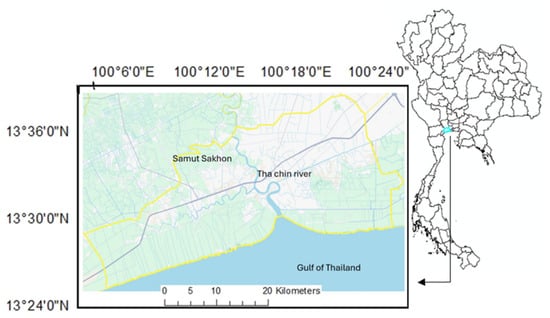
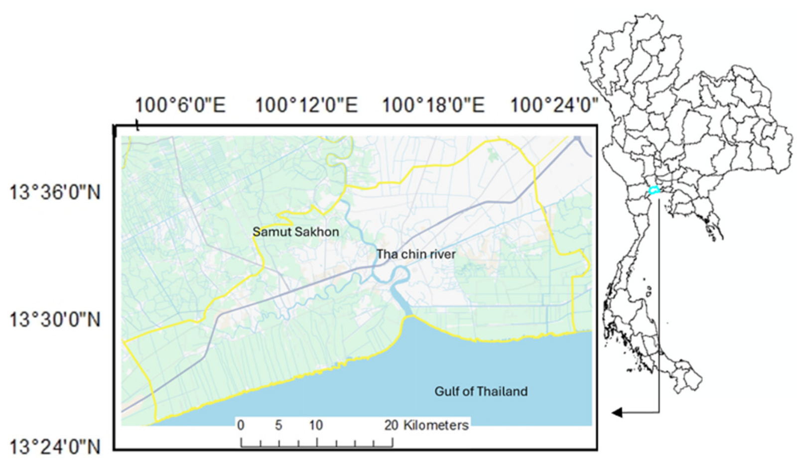
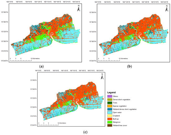
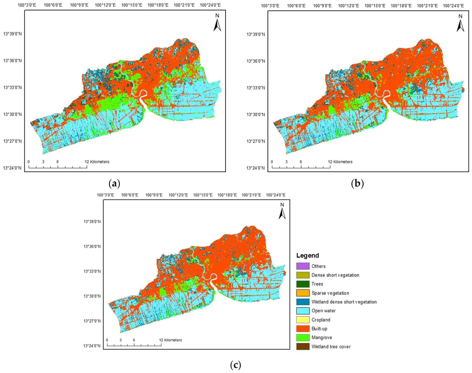
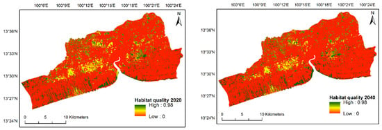
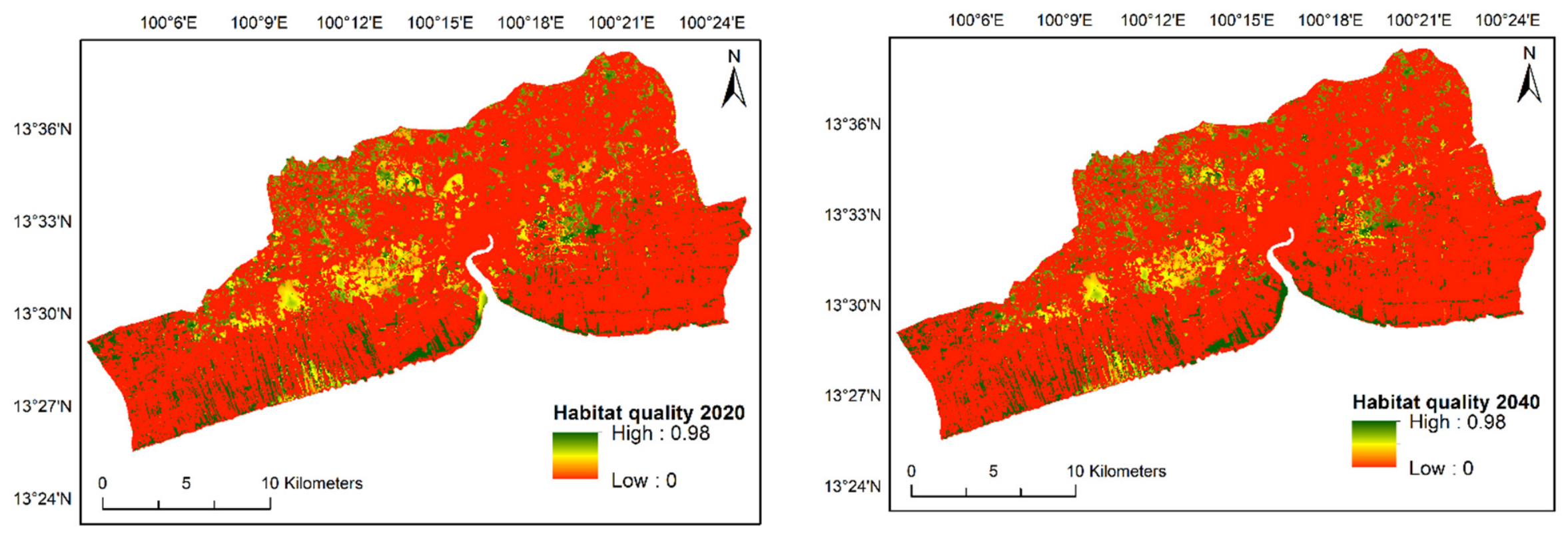
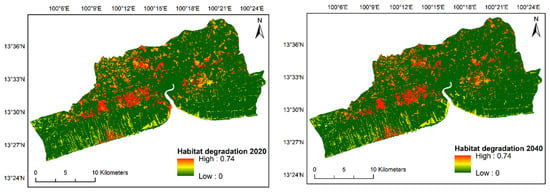
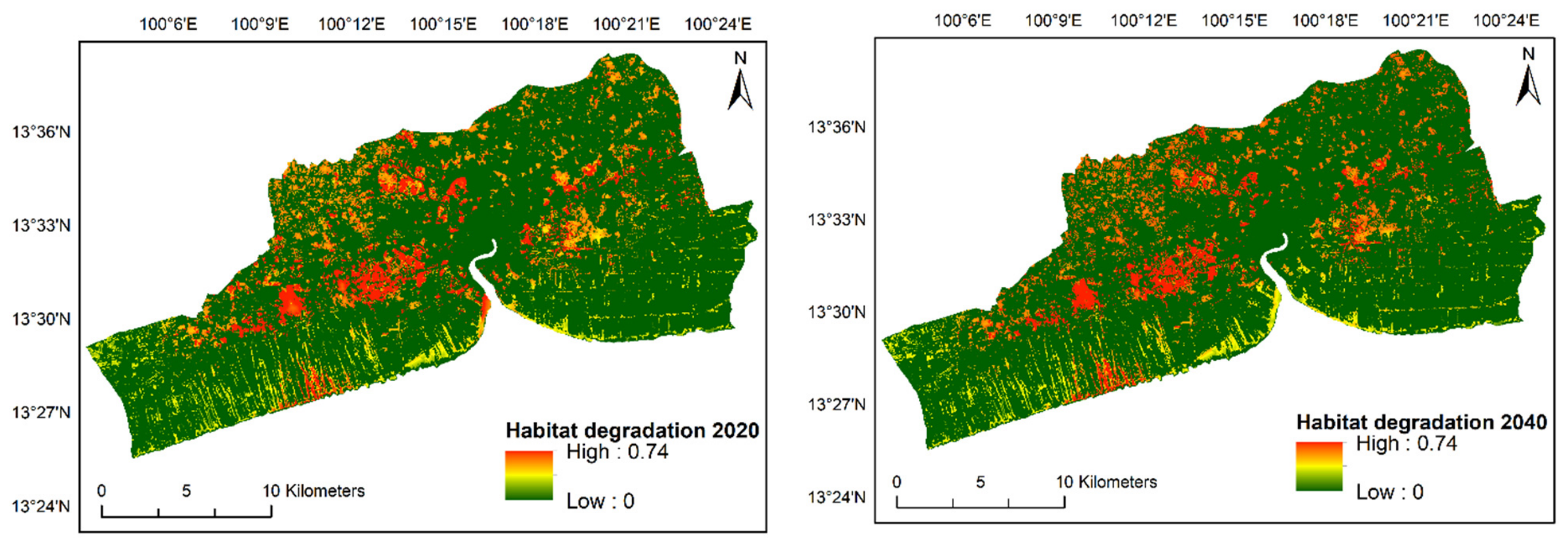
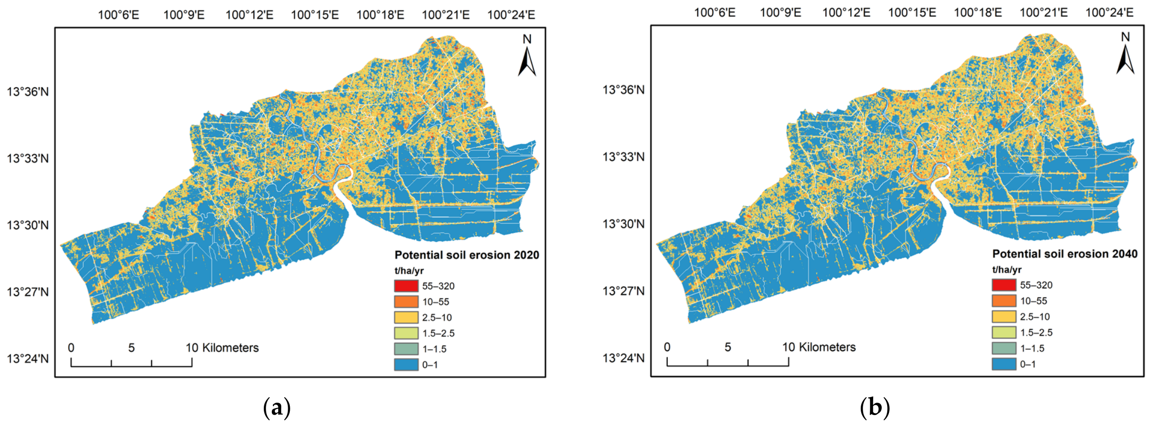
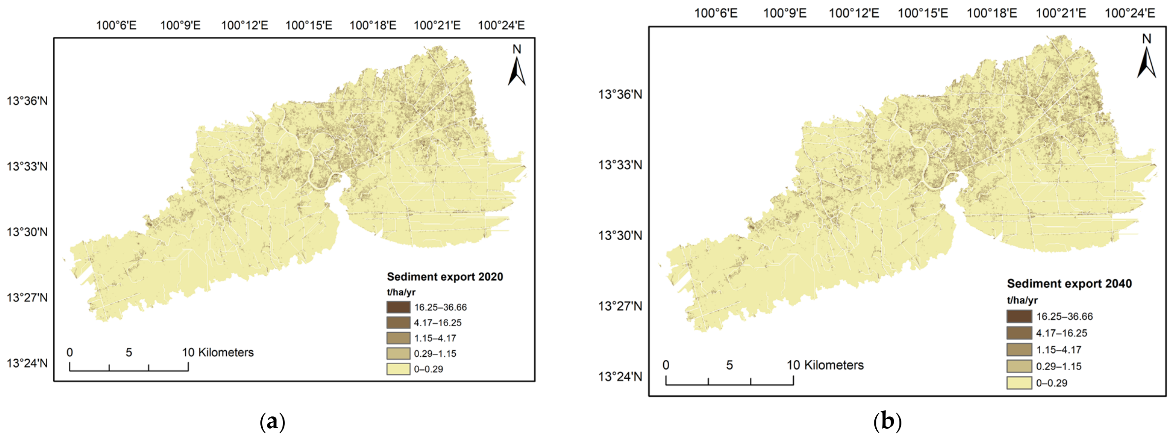
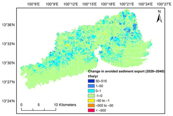
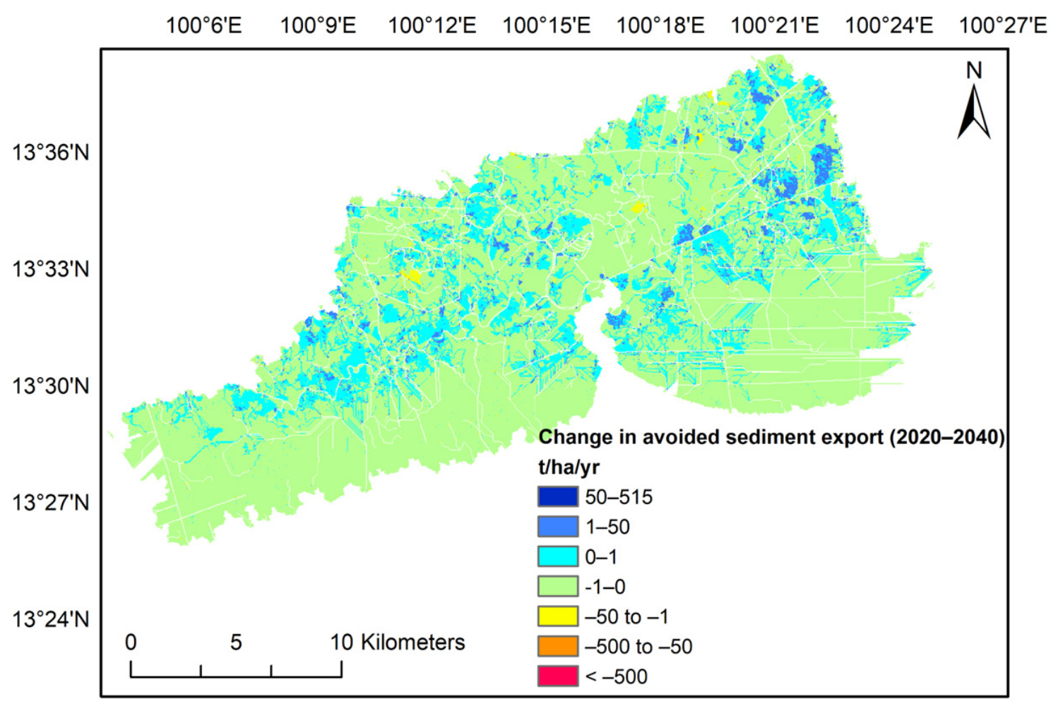

Disclaimer/Publisher’s Note: The statements, opinions and data contained in all publications are solely those of the individual author(s) and contributor(s) and not of MDPI and/or the editor(s). MDPI and/or the editor(s) disclaim responsibility for any injury to people or property resulting from any ideas, methods, instructions or products referred to in the content. |
© 2026 by the authors. Licensee MDPI, Basel, Switzerland. This article is an open access article distributed under the terms and conditions of the Creative Commons Attribution (CC BY) license.