


Abstract
Almaciga (Agathis philippinensis Warb.) is an ecologically and economically important forest tree in the Philippines, yet regional information on its environmental suitability remains limited. This study modeled current relative environmental suitability in the Davao Region using MaxEnt and a multicollinearity-controlled predictor-selection framework. From 504 assembled occurrence records, 1 km spatial thinning retained 36 records for modeling. Predictor screening reduced 20 climatic and topographic variables to maximum temperature of the warmest month (BIO5) and elevation. The model achieved training and testing AUC values of 0.8955 and 0.8415, respectively, indicating useful occurrence-background discrimination within the regional modeling domain. Elevation dominated the model, accounting for 95.28% of the contribution and 94.46% of the permutation importance. The retained occurrence records spanned 240–2804 m a.s.l., reflecting a broad regional elevational distribution. Higher predicted suitability was concentrated mainly in mountainous areas. The resulting map should be interpreted as a regional environmental-similarity and reconnaissance tool for guiding field verification rather than as evidence of confirmed occupancy or management suitability. Future validation should incorporate broader occurrence coverage and additional habitat and disturbance variables.
1. Introduction
The Philippines is recognized as a global biodiversity hotspot [1] with high levels of species richness and endemism occurring alongside continuing habitat loss and land-use pressure [2,3]. Forest ecosystems are particularly important because they support many endemic, threatened, and economically valuable plant species [4,5] and provide ecosystem services such as watershed protection [6], carbon storage [7,8], livelihood resources [4,9], and habitat connectivity [10,11]. However, conservation planning in forest landscapes requires more than species lists [12]; it also requires spatially explicit information on where suitable habitats occur [4,13], which environmental factors shape species distributions [4,14], and which areas should be prioritized for protection, restoration, or sustainable management [15]. This need is especially relevant in biodiversity-rich regions of the Philippines, where field data remain uneven and spatial documentation of biodiversity is still affected by geographic and taxonomic gaps [1,16,17,18].
Almaciga (Agathis philippinensis Warb.) is an ecologically and economically important forest tree species in the Philippines. It is valued for its resin, commonly known as Manila copal, which has been used in varnish, paint, incense, paint driers, and other industrial products [19,20]. Previous work on A. philippinensis has shown that resin tapping and collection practices vary across sites and that the species contributes to the supplemental income of local and Indigenous communities, including in sites such as Mt. Hamiguitan, Governor Generoso, Davao Oriental [21]. At the same time, unsustainable tapping, excessive bark injury, poor tapping skills, habitat disturbance, and limited information on suitable habitats may affect the long-term management of remaining populations [20,21,22]. For this reason, identifying where the species is most likely to occur under suitable environmental conditions is important for aligning conservation goals with sustainable forest use.
Despite the ecological and livelihood importance of A. philippinensis, regional-scale spatial information in the Davao Region remains limited. Existing evidence comes mainly from field observations, forest inventories, local management records, resin-quality studies, and site-specific studies [19,23]. The Davao region includes mountainous landscapes, forest fragments, protected areas, ancestral domains, and production landscapes [24,25]. Considering this characterized landscape, species-distribution modeling can provide a preliminary regional screening of current climatic-topographic similarity and identify areas for field validation [26,27,28]; current distribution does not by itself confirm occupancy, habitat condition, or suitability for protection, restoration, or planting; however, it increases chances of targeted surveys.
Species distribution models are useful tools for addressing this type of spatial conservation problem. These models relate species occurrence records to environmental predictors to estimate areas with suitable environmental conditions across a landscape [29]. Among these approaches, Maximum Entropy modeling, or MaxEnt, is widely used because it can model species distributions using presence-only occurrence data, which are common in biodiversity surveys and herbarium- or inventory-based datasets [30]. MaxEnt has been applied in ecological, conservation, and biogeographic studies because it can generate spatial predictions even when confirmed absence data are unavailable [31,32]. However, presence-only models must be interpreted carefully because they estimate relative habitat suitability rather than confirmed species occupancy, and their outputs may be influenced by sampling bias, background selection, predictor choice, and model settings [31,32].
A major methodological concern in species distribution modeling is multicollinearity, which occurs when two or more environmental predictors are strongly correlated [12,33,34,35]. In ecological models, collinearity can make it difficult to interpret the relative influence of predictors because variables may share overlapping information [34,36,37]. This issue is particularly common when using bioclimatic variables, many of which are derived from related temperature and precipitation measurements [12,28]. Although some studies suggest that machine-learning algorithms such as MaxEnt may maintain high predictive performance even when correlated variables are included, collinearity can still affect ecological interpretation, model stability, and transferability [33,36]. Therefore, predictor screening using correlation analysis [38,39], hierarchical clustering [40,41], and Variance Inflation Factor [42,43] can improve model parsimony and support clearer interpretation of the environmental drivers of species distribution.
This study aimed to model current relative environmental suitability for A. philippinensis in the Davao Region, Philippines, using a geospatial MaxEnt approach and a multicollinearity-controlled variable-selection framework. Specifically, the study sought to: (1) map current relative suitability within the Davao Region; (2) identify the relative influence of environmental predictors retained after screening 20 climatic and topographic variables; and (3) provide an initial spatial screening layer to guide field verification and future conservation planning.
2. Materials and Methods
2.1. Study Area and Occurrence Records
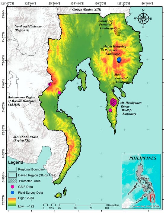
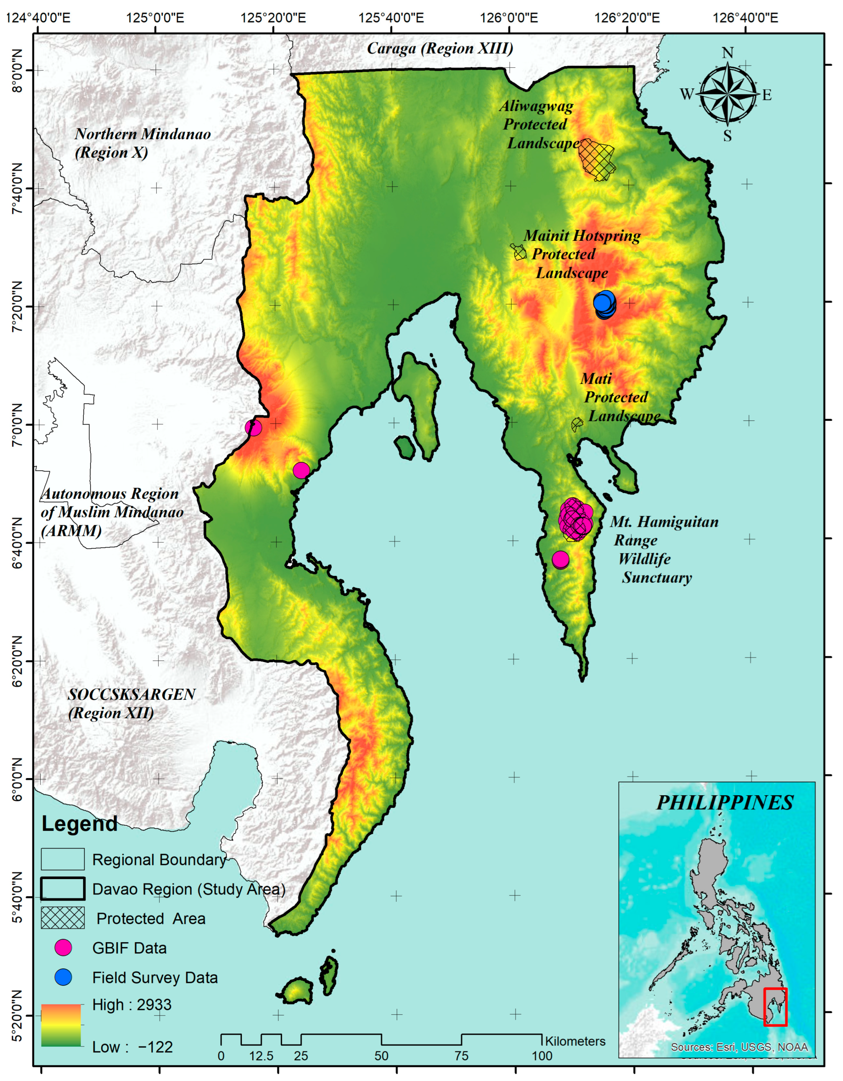
The study was conducted in the Davao Region (Region XI), southeastern Mindanao, Philippines (Figure 1). The administrative study extent includes Davao de Oro, Davao del Norte, Davao del Sur, Davao Occidental, and Davao Oriental. As of 31 July 2025, the region comprised six cities, 43 municipalities, and 1162 barangays [44]. Its coastal lowlands, interior valleys, uplands, and montane systems provide broad climatic and elevational gradients for regional habitat suitability assessment [25,45].
Figure 1.
Study area in the Davao Region (Region XI), Philippines, showing elevation, protected areas, surrounding administrative regions, and the 36 occurrence records retained after 1 km spatial thinning. The raw dataset comprised 463 field-survey records and 41 GBIF records; displayed points represent the modeling dataset rather than all known populations of Agathis philippinensis.
Occurrence records were obtained from GBIF (n = 298) [46]; following screening to exclude records falling outside the Davao Region, 41 records and 467 field-survey records were retained for analysis, for a total of 508 records before cleaning. Further, five repeated records were removed by exact coordinate de-duplication, leaving 503 unique occurrences as the final clean records used for spatial thinning. To reduce local oversampling, points were projected to WGS 84/UTM zone 51N (EPSG:32651) and thinned with the gridSample function in the R packages dismo and raster by retaining a maximum of one record per 1 km grid cell [47,48]. The generalized source-labelled occurrence records retained after spatial thinning are provided in Supplementary File S1. The R script used to implement the 1 km grid-based spatial thinning procedure is provided in Supplementary File S2. This thinning retained 36 records (7.10% of the assembled dataset): 27 attributable to GBIF and 9 to field sources. The thinned records were assigned to fixed training (n = 27) and testing (n = 9) files, a 75:25 holdout. Generalized versions of the fixed training and testing datasets, together with associated reproducibility information, are provided in Supplementary File S3. MaxEnt’s default duplicate-pixel filtering subsequently retained 24 unique training cells. Because several thinned records still occur within the same broad mountain landscapes, the holdout is not geographically independent; this limitation is addressed explicitly below [27,49,50]. Elevation values for the 36 thinned occurrence coordinates were extracted from the WorldClim 2.1 30-arc-second elevation raster using terra in R (version 4.6.2). The retained training and testing records were combined, converted to spatial points, and sampled using terra::extract(). Summary statistics were calculated in R, and the elevation distribution was visualized as a boxplot using ggplot2 and ggdist.
The target taxon was Almaciga, treated herein as Agathis philippinensis Warb. to maintain consistency with Philippine forestry and conservation literature, although major taxonomic resources recognize it as a synonym of the accepted name Agathis dammara (Lamb.) Rich. [51,52,53,54]. Published accounts report an elevational range of approximately 150–2200 m above sea level [54,55]; this was treated as contextual information only and not as the observed elevational distribution of the occurrence records retained for the present regional model. The species is assessed as Vulnerable on the IUCN Red List [52], and is included in the updated national list of threatened Philippine plants [56].
2.2. Environmental Predictors Selection
Twenty environmental predictors were used at a spatial resolution of 30 arc-seconds, corresponding to approximately 1 km. Nineteen bioclimatic variables were sourced from the WorldClim database Version 2.1, which provides global climate layers widely applied in ecological and species distribution modeling [57,58]. Elevation (ELEV) was included as a topographic predictor and derived from the Shuttle Radar Topography Mission (SRTM) digital elevation model, and also available from WorldClim [58,59]. The complete list of environmental predictors, including variable codes, full variable names, units, data sources, and ecological relevance, is provided in Supplementary File S4. These variables were chosen to represent the climatic and topographic conditions that may influence the distribution of Agathis philippinensis in the Davao Region.
Predictor screening was conducted using values extracted at the same 1000 random locations distributed across the Davao Region. The screening steps were applied in a fixed order. First, pairwise Pearson correlations were calculated. Second, predictors connected by |r| >= 0.70 were grouped using hierarchical clustering. Third, one representative per cluster was advanced on the basis of ecological interpretability, avoidance of redundant information, and representation of a distinct climatic or topographic dimension. Fourth, the candidate predictors entered iterative VIF screening, in which the highest-VIF variable was removed until all remaining VIF values were <= 5 [35,37,42,60]. The same 1000-point extraction was used throughout and was independent of the 10,014 MaxEnt background points. Intermediate VIF values were not retained. The Pearson-correlation and hierarchical-clustering reproducibility files are provided in Supplementary File S5.
2.3. Species Distribution Modeling
MaxEnt version 3.4.4 was run through the standalone Java application with BIO5 and ELEV as continuous layers at 30-arc-second resolution [31,57]. The model used cloglog output, 10,014 background points, automatic feature selection (linear, quadratic, and hinge features were fitted), the default regularization multiplier of 1, a maximum of 500 iterations, convergence after 320 iterations, one replicate, response-curve and jackknife outputs, and the fixed user-supplied training and testing files. MaxEnt’s random-seed option was not enabled. The accessible background was the set of cells with complete predictor data in the regional environmental layers. The MaxEnt run log and parameter coefficients are provided in Supplementary File S6.
The output is a relative suitability index, not a probability of occupancy, abundance estimate, or mapped population distribution. Higher cloglog values indicate environmental conditions more similar to those at the retained occurrence cells relative to conditions available in the selected background [30,32].
2.4. Model Evaluation and Variable Importance
Model discrimination was evaluated with the area under the Receiver Operating Characteristic Curve (AUC) [31,61]. In presence-background modeling, AUC measures ranking discrimination between occurrence and background sites; it does not measure classification accuracy [31,62,63]. Training and fixed-holdout testing AUCs were reported together with regularized gain, test gain, omission rates, and jackknife results. Because random or non-spatial holdouts can place environmentally and geographically similar records in both partitions, AUC was interpreted cautiously in light of residual clustering [49,50]. The corresponding model-evaluation outputs, including sample predictions, omission data, summary results, and predictor sample averages, are provided in Supplementary File S7.
2.5. Habitat Suitability Mapping
The continuous cloglog surface was retained as the primary model output (Supplementary File S8). For a binary screening layer, we used the 10th-percentile training-presence threshold (cloglog = 0.2108), which allows omission of a small proportion of calibration records and is less sensitive than a minimum-presence rule to geolocation or environmental error [64,65,66]. Five equal-width bands (0.0–0.2, 0.2–0.4, 0.4–0.6, 0.6–0.8, and 0.8–1.0) were used only to summarize and display gradients in the supplied regional map; they are cartographic bands and must not be interpreted as biologically validated presence/absence classes. Areas were calculated from the region-clipped raster using 0.852 km2 per grid cell.
3. Results and Discussion
3.1. Environmental Variables Selection
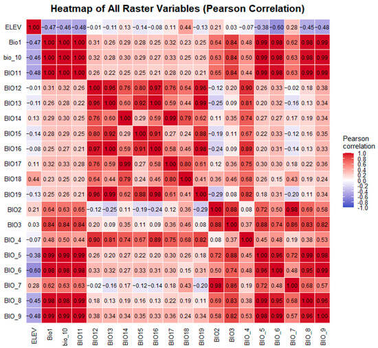
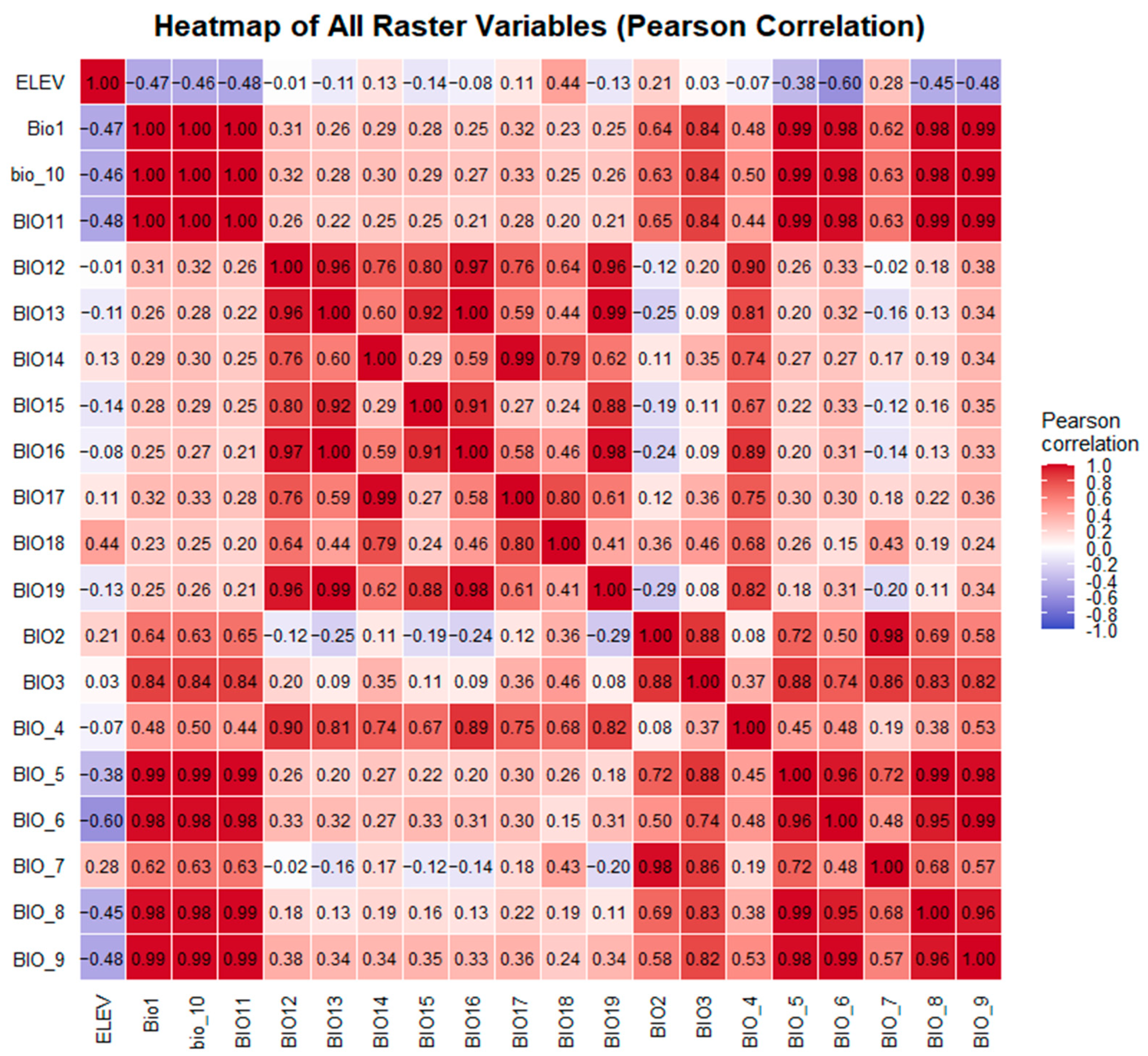
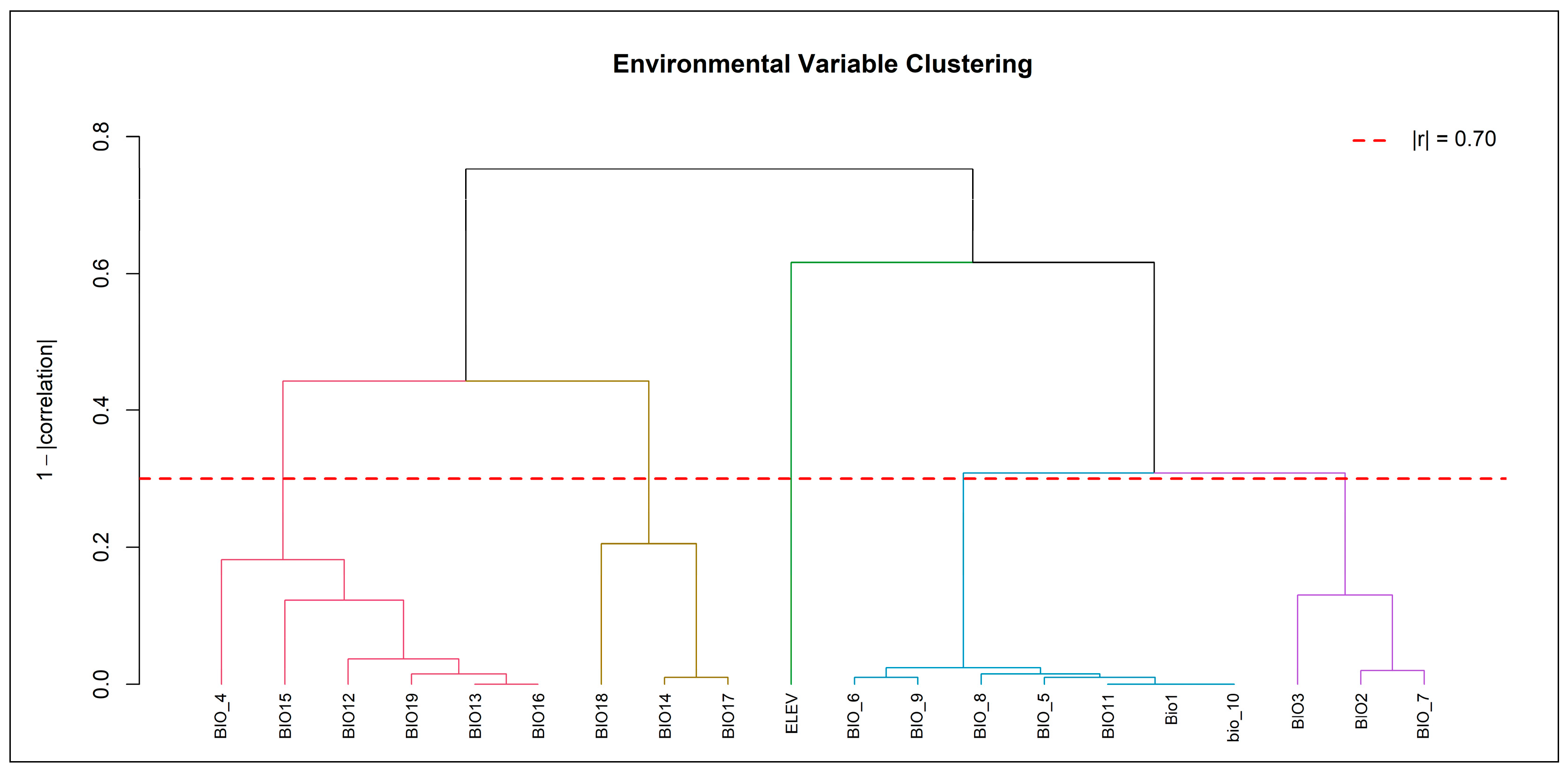
The 20 initial predictors were evaluated at the same 1000 regional random points. Pearson correlations and hierarchical clustering at |r| >= 0.70 identified five groups: a precipitation amount/seasonality group represented by BIO13; a dry/warm-quarter precipitation group represented by BIO18; a broad temperature group represented by BIO5; a diurnal-range/isothermality group represented by BIO3; and elevation as a separate topographic group (Figure 2 and Table 1). These five representatives entered VIF screening (Table 2). BIO13, BIO18, and BIO3 were removed iteratively, leaving BIO5 and ELEV, each with a final VIF of 1.731 (Table 3). The screening improves parsimony but does not show that excluded precipitation variables are ecologically unimportant; it shows only that they were redundant under the selected regional layers and decision rules [28,35,36].
Figure 2.
Pearson correlation heatmap for the 20 environmental predictors, calculated from predictor values extracted at 1000 random locations across the Davao Region.
Table 1.
Predictor clusters at |r| >= 0.70 and representatives advanced to iterative VIF screening.
Table 2.
Outcome of iterative VIF screening for the five cluster representatives and final VIF values for retained predictors.
Table 3.
MaxEnt percent contribution and permutation importance for the two retained predictors.
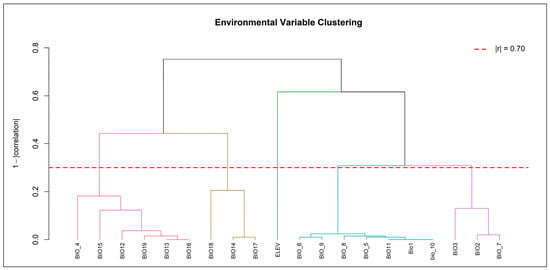
Hierarchical clustering was used to organize correlated predictors rather than to claim causal ecological groupings (Figure 3). The representative retained from each cluster and its subsequent VIF screening outcome are reported in Table 1 and Table 2. This explicit sequence resolves the previously inconsistent description of correlation thresholds and distinguishes correlation screening from the independent MaxEnt background sample.
Figure 3.
Hierarchical clustering dendrogram of the 20 candidate predictors using correlations calculated from the common set of 1000 regional random points. The cut at |r| >= 0.70 identified the five groups summarized in Table 1.
The full post-clustering candidate set was BIO13, BIO18, BIO5, BIO3, and ELEV. Iterative VIF screening removed BIO13, BIO18, and BIO3 and retained BIO5 and ELEV. The archived analysis records final VIF = 1.731 for both retained variables but does not contain the intermediate VIF values for eliminated candidates.
The two-variable model is intentionally parsimonious but ecologically incomplete. Elevation can covary with temperature, cloud exposure, moisture, topography, forest type, soils, and accessibility [67,68], while BIO5 represents only one thermal extreme [69,70]. The omission of direct precipitation, soil, land-cover, forest-structure, slope, aspect, evapotranspiration, road, and disturbance variables limits causal interpretation. Recent tree-distribution studies illustrate that broader predictor sets and ensemble or future-scenario designs can address different questions [47,71,72]; those additional analyses were outside the data available for this regional current-condition model.
3.2. Model Performance and Predictor Influence
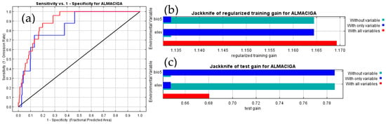
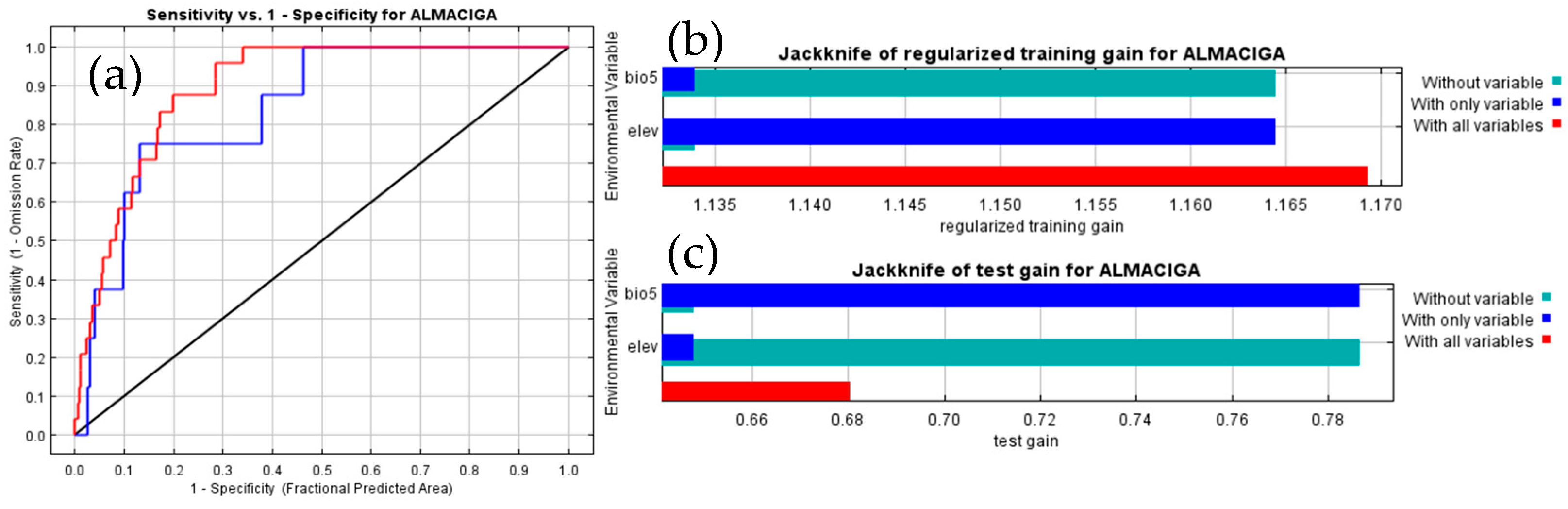
Elevation accounted for 95.2839% of model training improvement and 94.4599% of permutation importance, whereas BIO5 accounted for 4.7161% and 5.5401%, respectively. These percentages should be interpreted together with the jackknife results. When fitted alone, elevation produced a regularized training gain of 1.1645 and BIO5 produced 1.1340, compared with 1.1693 for the full model (Figure 4b). Thus, adding BIO5 to elevation increased training gain by only 0.0048, while adding elevation to BIO5 increased it by 0.0353. The two predictors therefore recovered much of the same regional presence-background separation when fitted independently, despite their final linear VIF of 1.731. This apparent contrast is not contradictory: VIF evaluates linear dependence among the raw predictors, whereas MaxEnt contribution and jackknife metrics depend on fitted features, the selected background, and the optimization path [31,32,36]. Accordingly, the contribution percentages are properties of this fitted model, not ecological effect sizes or evidence of direct causal control.
Figure 4.
Summary of model performance and influence: (a) Receiver Operating Characteristic; (b) jackknife regularized training gain for single-predictor and full models; and (c) presence-background AUC for the training and fixed testing sets.
The dominance of elevation nevertheless shows that the mapped surface is organized primarily along a regional topographic gradient. For A. philippinensis, this is consistent with its documented association with upland forest environments [19,20,54,73], but elevation is an integrative spatial surrogate rather than a resource used directly by the tree. Across tropical mountains, elevation can covary with air temperature, cloud exposure, moisture balance, soil development, terrain, forest type, and human accessibility, and the form of these relationships can vary among landscapes [74]. The small conditional contribution of BIO5 therefore means that maximum warm-season temperature added limited information after elevation was included; it does not demonstrate that heat is ecologically unimportant. Because precipitation, forest structure, land cover, soils, and disturbance were not retained or supplied, the model cannot separate their effects from the elevation-associated pattern. The result is best understood as a parsimonious model of regional environmental similarity, not a complete representation of the species’ niche.
Training AUC was 0.8955 and testing AUC was 0.8415, a difference of 0.0540, with a test-AUC standard deviation of 0.0556 (Figure 4c). The holdout set therefore retained useful ranking discrimination within the selected regional background, but the precision of that estimate is limited. AUC measures how occurrences are ranked relative to background sites and is not classification accuracy [63,75]. Moreover, only eight test records entered evaluation, so each record represented 12.5% of the test omission calculation. At the 10th-percentile threshold, the reported test omission of 0.2500 corresponds to two omitted test records, compared with two of 24 training records (0.0833). This difference is a direct indication that the threshold transferred less consistently to the small holdout than to the calibration data. Because the split was non-spatial and both partitions came from the same clustered mountain landscapes, neither the AUC nor omission results establish transferability to unsampled mountain systems [49,50]. They support cautious within-region ranking, subject to the occurrence sampling and background assumptions of presence-background models [69,76].
3.3. Elevation Distribution of Thinned Occurrence Records
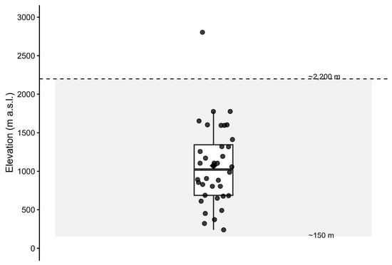
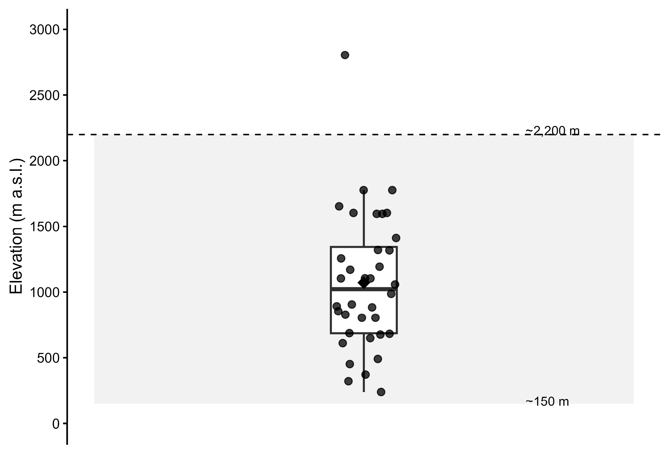
Elevation values for the 36 spatially thinned occurrence records were extracted from the WorldClim 2.1 30-arc-second elevation raster using the terra package in R. The distribution was summarized using descriptive statistics and visualized as a boxplot with ggplot2 and ggdist, combining a half-density plot, boxplot, individual jittered points, and a mean marker. The published species-level elevational range of approximately 150–2200 m a.s.l. [20,54] was shown as a contextual reference band.
Elevation ranged from 240 to 2804 m a.s.l. (mean = 1072 m; median = 1023 m; IQR = 686–1343 m; Figure 5). The extracted elevation values, descriptive statistics, R workflow, and outputs are provided in Supplementary File S9. The middle 50% of records spanned 657 m, with occurrences also extending below and above this central range. Records below 1000 m indicate that the model response should not be interpreted as a hard lower elevational limit, while the 2804 m maximum exceeds the published upper range and should be interpreted cautiously in relation to locality accuracy and raster-cell elevation. More broadly, the elevation response reflects the distribution of thinned regional records relative to the available environmental background rather than a physiological optimum [32,67].
Figure 5.
Elevational distribution of the 36 spatially thinned occurrence records of Agathis philippinensis in the Davao Region, Philippines. Individual points represent retained occurrence records, the boxplot summarizes their elevational distribution, the box indicates the interquartile range (686–1343 m), the central line represents the median (1023 m), and the diamond denotes the mean (1072 m). The shaded area indicates the approximate published species-level elevational range of 150–2200 m.
3.4. Regional Habitat Suitability Pattern
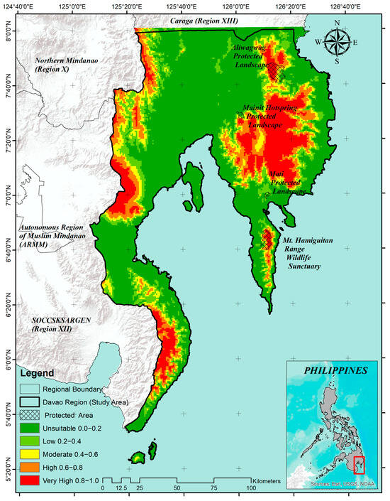
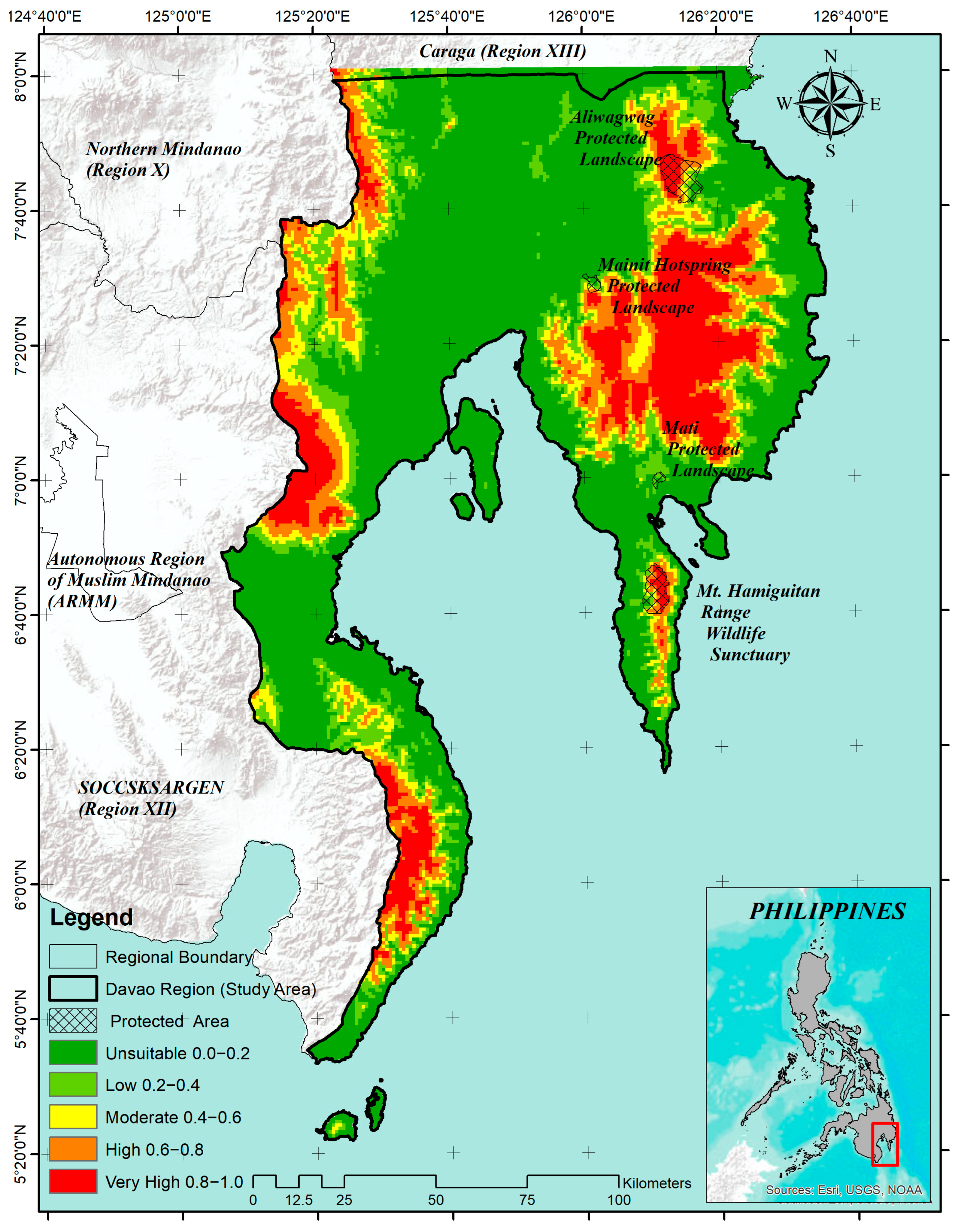
The overlayed map shows a heterogeneous but strongly elevation-associated suitability pattern (Figure 6). Across 19,315.692 km2 represented by 22,671 grid cells, 56.88% of the mapped area fell in the 0.0–0.2 display band, while 43.12% fell in the four higher display bands combined (Table 4). The latter percentage must not be interpreted as the area of suitable habitat because the independently selected 10th-percentile training-presence threshold was 0.2108, which cuts within the 0.2–0.4 band. The equal-width bands serve cartographic communication, whereas the threshold provides a separate screening rule [65,77]. At that threshold, two of 24 training records and two of eight evaluated test records were omitted. The contrast indicates that the threshold retained most calibration environments but was less stable in the small holdout. Thresholded area should consequently be treated as a hypothesis about environmental similarity, not a binary estimate of occupied habitat.
Figure 6.
Final MaxEnt habitat suitability output for Agathis philippinensis in the Davao Region (Region XI), Philippines, showing protected areas, surrounding administrative regions, and continuous cloglog suitability values displayed in five descriptive classes for visualization.
Table 4.
Area of descriptive relative suitability classes within the Davao Region after overlay with the regional boundary.
Higher suitability bands occur mainly along mountainous parts of the Davao Region. Given the overwhelming elevation contribution, these areas are most defensibly interpreted as upland environmental analogs of the retained occurrence sites. This is still useful for survey design: high-value cells can identify candidate landscapes for reconnaissance, whereas selected low-value and under-sampled elevational strata provide necessary tests of model commission and omission. The protected-area overlay shows that some predicted areas intersect or adjoin established protected landscapes, but it is contextual rather than a quantitative gap analysis. Legal protection also does not by itself demonstrate suitable forest condition, effective management, or the presence of viable Almaciga populations [17,18]. For a resin-producing tree, site-level decisions additionally require information on stand density, size-class structure, regeneration, tree health, tapping history, access, and tenure [21,22,23]. Similarly, restoration or enrichment planting requires current forest and land-use data, soils, planting-material provenance, disturbance risk, and local management feasibility. The model should therefore be used as the first stage of a sequential assessment—regional screening, field verification, habitat and tenure evaluation, and only then conservation or restoration prioritization—rather than as a stand-alone decision surface [61,69,78].
3.5. Limitations of the Study
Several limitations define the scope of these findings. First, the 508 assembled records were strongly clustered, especially around Mt. Hamiguitan and the Maragusan-New Bataan area. One-kilometer thinning reduced repeated local weighting to 36 records but did not make geographic coverage representative; spatial filtering cannot recover information from unsurveyed landscapes. Second, the fixed 75:25 holdout was non-spatial. It tests separation of records within the sampled data structure, not prediction to independent mountain systems, and may leave AUC optimistic where nearby sites share environmental and spatial structure. Third, the accessible background was defined by the regional predictor layers and was not corrected with a target-group or survey-effort bias surface, so a different background could change fitted contrasts. Fourth, the final model contains only elevation and BIO5; the dominant elevation contribution likely combines multiple omitted climatic, habitat, and accessibility gradients. Fifth, no forest cover, land-use, roads, soils, terrain derivatives, disturbance, population status, or quantitative protected-area coverage was analyzed. Finally, no future SSP projection was performed. The results therefore describe current relative environmental suitability under the supplied layers and do not support future range-shift, climate-adaptation, confirmed occupancy, population viability, or planting-feasibility claims.
A stronger next phase should collect geographically independent records from underrepresented provinces and mountain systems, stratifying surveys across elevation and predicted-value classes rather than concentrating only on mapped high values. Once sample coverage is sufficient, spatial-block or leave-one-landscape-out validation can test transferability; bias-aware backgrounds can be compared with the regional background; and land cover, forest structure, soil, terrain, hydrology, roads, and disturbance can be evaluated as explicit predictors. These additions would allow the model to be judged against the intended management application rather than by discrimination statistics alone. Until such validation is available, the present output is appropriately used as a regional reconnaissance and hypothesis-generating layer.
4. Conclusions
This study developed a parsimonious MaxEnt model of the current relative environmental suitability of Agathis philippinensis in the Davao Region using spatially thinned occurrence records and multicollinearity-controlled predictor selection. Of 504 assembled records, 36 were retained after 1 km spatial thinning and partitioned into 27 training and 9 testing records. MaxEnt evaluated 24 unique training cells and eight testing records, producing training and testing AUC values of 0.8955 and 0.8415, respectively. These values indicate useful occurrence-background discrimination within the regional modeling domain but should not be interpreted as classification accuracy or evidence of geographically independent transferability.
Elevation dominated the fitted model, accounting for 95.2839% of percent contribution and 94.4599% of permutation importance, while BIO5 contributed 4.7161% and 5.5401%, respectively. The resulting suitability surface was therefore structured mainly along the regional elevational gradient, although elevation should be interpreted as an integrative environmental surrogate rather than a direct ecological determinant. The 36 thinned occurrence records spanned 240–2804 m a.s.l. (mean = 1072 m; median = 1023 m; IQR = 686–1343 m), indicating a broad regional elevational distribution. Because the maximum raster-derived elevation exceeds the published species-level range of approximately 150–2200 m, this value should be interpreted cautiously.
The continuous cloglog surface should remain the primary model output, while the 10th-percentile training-presence threshold of 0.2108 provides a reproducible binary screening rule. The five equal-width bands are intended only for visualizing relative environmental gradients and should not be treated as biologically validated presence–absence classes. Higher predicted values were concentrated mainly in mountainous areas and should be regarded as candidate locations for field verification rather than confirmed populations or automatically suitable sites for conservation, restoration, or enrichment planting.
Overall, the model is best used as a regional reconnaissance and hypothesis-generating tool. Interpretation remains constrained by the small, thinned sample, residual spatial clustering, non-spatial holdout design, regional background definition, and the limited final predictor set of elevation and BIO5. Future work should expand geographically independent occurrence sampling, apply spatially structured validation, test alternative background and regularization settings, and incorporate additional predictors such as forest cover, land-use, soils, terrain, hydrology, roads, disturbance, and population-status data. Because no future climate scenarios were analyzed, the results should be restricted to current relative environmental suitability and should not be used to infer future range shifts or climate-change responses.
Supplementary Materials
The following supporting information can be downloaded at: https://www.mdpi.com/article/10.3390/ecologies7040109/s1. The materials comprise: File S1, generalized source-labelled occurrence records; File S2, R script for 1-km spatial thinning; File S3, generalized fixed training and testing partitions and reproducibility information; File S4, environmental predictor variables; File S5, Pearson-correlation and hierarchical-clustering reproducibility files; File S6, final MaxEnt run log and parameter coefficients; File S7, sample predictions, omission data, and MaxEnt model-evaluation outputs; File S8, continuous region-clipped cloglog suitability raster; and File S9, elevation extraction, descriptive statistics, R workflow, and Figure 5 supporting materials. The GBIF occurrence records used in the study were obtained from GBIF.org (26 August 2026), GBIF Occurrence Download, https://doi.org/10.15468/dL.3zbb3h. Exact occurrence coordinates are withheld from the publicly accessible supplementary package and are managed under controlled-access conservation data-sharing safeguards.
Author Contributions
Conceptualization, J.S.C., L.B.B. and A.G.P.; methodology, J.S.C.; formal analysis and visualization, J.S.C. and R.M.A.; writing—original draft preparation, review and editing, L.B.B. and J.S.C. All authors have read and agreed to the published version of the manuscript.
Funding
This research was funded by the Global Environment Facility (GEF) through the Department of Environment and Natural Resources (DENR)–United Nations Development Programme (UNDP) Biodiversity Corridor Project (UNDP-GEF-PIMS ID No 5886), under the Eastern Mindanao Biodiversity Corridor (EMBC) Clusters 5 and 6 implemented by Davao Oriental State University.
Data Availability Statement
The data and reproducibility materials supporting this study are publicly available in Zenodo at https://doi.org/10.5281/zenodo.22711236. The GBIF occurrence records used in the analysis are available from GBIF.org (26 August 2026), GBIF Occurrence Download, https://doi.org/10.15468/dL.3zbb3h. Exact coordinates of sensitive occurrence localities are not publicly disclosed and are managed under controlled-access conservation data-sharing safeguards.
Acknowledgments
The authors acknowledge the partial support provided by the Davao Oriental State University internal research fund. The authors also extend their genuine appreciation to their colleagues and friends in the academe for their valuable support, and to the Department of Environment and Natural Resources (DENR) for issuing the Gratuitous Permit (WGP No. XI-2025-064), which facilitated the field survey data used in this study. During the preparation of this manuscript, the authors used Grammarly Premium to ensure proper writing and grammar. The authors have reviewed and edited the output and take full responsibility for the content of this publication. Finally, the authors sincerely thank the anonymous reviewers for their substantial comments, which greatly contributed to the refinement and improvement of this work.
Conflicts of Interest
The authors declare no conflicts of interest. The funders had no role in the design of the study; in the collection, analyses, or interpretation of data; in the writing of the manuscript; or in the decision to publish the results.
Abbreviations
The following abbreviations are used in this manuscript:
| Abbreviation | Full Term |
| A. philippinensis | Agathis philippinensis |
| AUC | Area Under the Receiver Operating Characteristic Curve |
| BIO | Bioclimatic variable |
| BIO1-BIO19 | WorldClim bioclimatic variables |
| BIO5 | Maximum Temperature of the Warmest Month |
| DEM | digital elevation model |
| DENR | Department of Environment and Natural Resources |
| DorSU | Davao Oriental State University |
| ELEV | elevation |
| EMBC | Eastern Mindanao Biodiversity Corridor |
| GBIF | Global Biodiversity Information Facility |
| GEF | Global Environment Facility |
| GIS | Geographic Information System |
| IUCN | International Union for Conservation of Nature |
| MaxEnt | Maximum Entropy |
| PRS | Philippine Reference System |
| ROC | Receiver Operating Characteristic |
| SDM | species distribution modeling |
| UNDP | United Nations Development Programme |
| UTM | Universal Transverse Mercator |
| VIF | Variance Inflation Factor |
| VU | Vulnerable |
References
- Amoroso, V.B.; Orias, P.J.F.; Taer, E.C.; Montero, Y.P.M. A Review of Philippine Plant Discoveries in the Last 25 Years. J. Nat. Conserv. 2026, 93, 127337. [Google Scholar] [CrossRef] [Scilit]
- Myers, N.; Mittermeier, R.A.; Mittermeier, C.G.; Da Fonseca, G.A.B.; Kent, J. Biodiversity Hotspots for Conservation Priorities. Nature 2000, 403, 853–858. [Google Scholar] [CrossRef] [Scilit] [PubMed]
- Posa, M.R.C.; Diesmos, A.C.; Sodhi, N.S.; Brooks, T.M. Hope for Threatened Tropical Biodiversity: Lessons from the Philippines. BioScience 2008, 58, 231–240. [Google Scholar] [CrossRef] [Scilit]
- Wani, A.M.; Sahoo, G. Forest Ecosystem Services and Biodiversity. In Spatial Modeling in Forest Resources Management; Shit, P.K., Pourghasemi, H.R., Das, P., Bhunia, G.S., Eds.; Environmental Science and Engineering; Springer: Cham, Switzerland, 2021; pp. 529–552. [Google Scholar]
- Brockerhoff, E.G.; Barbaro, L.; Castagneyrol, B.; Forrester, D.I.; Gardiner, B.; González-Olabarria, J.R.; Lyver, P.O.; Meurisse, N.; Oxbrough, A.; Taki, H.; et al. Forest Biodiversity, Ecosystem Functioning and the Provision of Ecosystem Services. Biodivers. Conserv. 2017, 26, 3005–3035. [Google Scholar] [CrossRef] [Scilit]
- Luck, G.W.; Chan, K.M.A.; Fay, J.P. Protecting Ecosystem Services and Biodiversity in the World’s Watersheds. Conserv. Lett. 2009, 2, 179–188. [Google Scholar] [CrossRef] [Scilit]
- Lyu, M.; Xie, J.; Giardina, C.P.; Vadeboncoeur, M.A.; Feng, X.; Wang, M.; Ukonmaanaho, L.; Lin, T.-C.; Kuzyakov, Y.; Yang, Y. Understory Ferns Alter Soil Carbon Chemistry and Increase Carbon Storage during Reforestation with Native Pine on Previously Degraded Sites. Soil Biol. Biochem. 2019, 132, 80–92. [Google Scholar] [CrossRef] [Scilit]
- Ojea, E.; Loureiro, M.L.; Alló, M.; Barrio, M. Ecosystem Services and REDD: Estimating the Benefits of Non-Carbon Services in Worldwide Forests. World Dev. 2016, 78, 246–261. [Google Scholar] [CrossRef] [Scilit]
- Negi, V.S.; Maikhuri, R.K.; Rawat, L.S. Non-Timber Forest Products (NTFPs): A Viable Option for Biodiversity Conservation and Livelihood Enhancement in Central Himalaya. Biodivers. Conserv. 2011, 20, 545–559. [Google Scholar] [CrossRef] [Scilit]
- Bai, Y.; Zhao, J.; Shen, H.; Li, X.; Wen, B. The Evolution of Forest Landscape Connectivity and Ecological Network Construction: A Case Study of Zhejiang’s Ecological Corridors. Sustainability 2024, 16, 5868. [Google Scholar] [CrossRef] [Scilit]
- Zhang, Y.; Luo, Y.; Han, L.; Chen, K.; Wang, Z.; Yang, Q. Importance of Patches in Maintaining Forest Landscape Connectivity: A Case Study of Barluk, Xinjiang, China. Forests 2025, 16, 74. [Google Scholar] [CrossRef] [Scilit]
- Baskent, E.Z.; Borges, J.G.; Kašpar, J. An Updated Review of Spatial Forest Planning: Approaches, Techniques, Challenges, and Future Directions. Curr. For. Rep. 2024, 10, 299–321. [Google Scholar] [CrossRef] [Scilit]
- Vázquez-Benito, J.A.; Burgos-Hernández, M.; López-Mata, L.; Galván-Escobedo, I.G.; Mata-Rosas, M.; Aguirre-Dugua, X. Beyond Protected Areas: Spatial Conservation Priorities for an Endemic and Endangered Orchid Species in Mexico Using Species Distribution Models. Front. Conserv. Sci. 2026, 7, 1777677. [Google Scholar] [CrossRef] [Scilit]
- Wang, H.-H.; Wonkka, C.L.; Treglia, M.L.; Grant, W.E.; Smeins, F.E.; Rogers, W.E. Species Distribution Modelling for Conservation of an Endangered Endemic Orchid. AoB Plants 2015, 7, plv039. [Google Scholar] [CrossRef] [Scilit] [PubMed]
- Duarte, G.T.; Ribeiro, M.C.; Paglia, A.P. Ecosystem Services Modeling as a Tool for Defining Priority Areas for Conservation. PLoS ONE 2016, 11, e0154573. [Google Scholar] [CrossRef] [Scilit] [PubMed]
- Berba, C.M.P.; Matias, A.M.A. State of Biodiversity Documentation in the Philippines: Metadata Gaps, Taxonomic Biases, and Spatial Biases in the DNA Barcode Data of Animal and Plant Taxa in the Context of Species Occurrence Data. PeerJ 2022, 10, e13146. [Google Scholar] [CrossRef] [Scilit] [PubMed]
- Mallari, N.A.D.; Collar, N.J.; McGowan, P.J.K.; Marsden, S.J. Philippine Protected Areas Are Not Meeting the Biodiversity Coverage and Management Effectiveness Requirements of Aichi Target 11. Ambio 2016, 45, 313–322. [Google Scholar] [CrossRef] [Scilit] [PubMed]
- Agduma, A.R.; Garcia, F.G.; Cabasan, M.T.; Pimentel, J.; Ele, R.J.; Rubio, M.; Murray, S.; Hilario-Husain, B.A.; Dela Cruz, K.C.; Abdullah, S.; et al. Overview of Priorities, Threats, and Challenges to Biodiversity Conservation in the Southern Philippines. Reg. Sustain. 2023, 4, 203–213. [Google Scholar] [CrossRef] [Scilit]
- Razal, R.A.; Jara, A.A.; Samar, G.P.O.; Alomia, R.L.M.; Taghap, K.M.; Agonia, M.R.; Rendon, M.D.D. Geographical Variations and Correlation among Some Chemical and Thermal Properties of Almaciga (Agathis philippinensis Warb.) Resins from Selected Commercial Sites in the Philippines. Heliyon 2021, 7, e06413. [Google Scholar] [CrossRef] [Scilit] [PubMed]
- Centre for Sustainability PH, Inc.; Forest Foundation Philippines. Almaciga Manual: Phenology, Economic Use, Ecology, Collection, Propagation, Reforestation; Forest Foundation Philippines: Makati, Philippines, 2017. [Google Scholar]
- Daracan, V.; Mendoza, R.; Torres, A.; Jara, A.; Manalo, R.; Batallones, C.H.; Razal, R. Comparison of Agathis philippinensis Resin Tapping and Collection Practices in Three Selected Sites in the Philippines. Biodiversitas 2020, 21, 5595–5604. [Google Scholar] [CrossRef] [Scilit]
- Ella, A.B.; Samiano, F.B. Enhancing the Adaptive Capacity of Indigenous Peoples by Promoting Sustainable Resin Tapping of Almaciga (Agathis philippinensis) in Palawan and Sierra Madre, Philippines; Southeast Asian Regional Center for Graduate Study and Research in Agriculture (SEARCA): Los Baños, Philippines, 2015. [Google Scholar]
- Evangelista, K.P.; Predo, C.; Andrada, R., II; Codilan, A.; Palma-Torres, V.; Amada, L.A.; Calderon, M. Supply Chain Analysis of Almaciga (Agathis philippinensis Warb.) Resin in Governor Generoso, Davao Oriental, Philippines. Ecosyst. Dev. J. 2022, 11, 13–20. [Google Scholar]
- Ramos, R.L.; Nemenzo-Calica, P.; Antonio, E.S. Elevation-Driven Shifts in Species Diversity, Endemicity, and Vegetation Structure across the Mount Hamiguitan Range Wildlife Sanctuary, a UNESCO World Heritage Site in Davao Oriental, Philippines. Davao Res. J. 2026, 17, 60–72. [Google Scholar] [CrossRef] [Scilit]
- Luna, T.W., Jr. Physical Aspects and Natural Resources of the Philippines. Philipp. Rev. Econ. 1965, 2, 28–53. [Google Scholar]
- Delos Angeles, M.D.; Radbouchoom, S.; Ngarega, B.K.; Lapuz, R.S.; Schneider, H. Spatial Diversity and Distribution of Fern and Lycophyte Species in Karst and Non-Karst Landscapes towards Conservation Needs. Front. Plant Sci. 2025, 16, 1495796. [Google Scholar] [CrossRef] [Scilit] [PubMed]
- Fourcade, Y.; Engler, J.O.; Rödder, D.; Secondi, J. Mapping Species Distributions with MAXENT Using a Geographically Biased Sample of Presence Data: A Performance Assessment of Methods for Correcting Sampling Bias. PLoS ONE 2014, 9, e97122. [Google Scholar] [CrossRef] [Scilit] [PubMed]
- Van Steenderen, C.J.M.; Sutton, G.F. Climate Covariate Selection Influences MaxEnt Model Predictions and Predictive Accuracy under Current and Future Climates. Ecol. Model. 2024, 498, 110872. [Google Scholar] [CrossRef] [Scilit]
- Elith, J.; Leathwick, J.R. Species Distribution Models: Ecological Explanation and Prediction Across Space and Time. Annu. Rev. Ecol. Evol. Syst. 2009, 40, 677–697. [Google Scholar] [CrossRef] [Scilit]
- Phillips, S.J.; Anderson, R.P.; Schapire, R.E. Maximum Entropy Modeling of Species Geographic Distributions. Ecol. Model. 2006, 190, 231–259. [Google Scholar] [CrossRef] [Scilit]
- Elith, J.; Phillips, S.J.; Hastie, T.; Dudík, M.; Chee, Y.E.; Yates, C.J. A Statistical Explanation of MaxEnt for Ecologists: Statistical Explanation of MaxEnt. Divers. Distrib. 2011, 17, 43–57. [Google Scholar] [CrossRef] [Scilit]
- Merow, C.; Smith, M.J.; Silander, J.A. A Practical Guide to MaxEnt for Modeling Species’ Distributions: What It Does, and Why Inputs and Settings Matter. Ecography 2013, 36, 1058–1069. [Google Scholar] [CrossRef] [Scilit]
- De Marco, P.; Nóbrega, C.C. Evaluating Collinearity Effects on Species Distribution Models: An Approach Based on Virtual Species Simulation. PLoS ONE 2018, 13, e0202403. [Google Scholar] [CrossRef] [Scilit] [PubMed]
- Naimi, B. On Uncertainty in Species Distribution Modelling. Ph.D. Thesis, University of Twente, Enschede, The Netherlands, 2015. [Google Scholar]
- Díaz-Vallejo, M.; Peña-Peniche, A.; Mota-Vargas, C.; Piña-Torres, J.; Valencia-Rodríguez, D.; Rangel-Rivera, C.E.; Gaviria-Hernández, J.; Rojas-Soto, O. Analyses of the Variable Selection Using Correlation Methods: An Approach to the Importance of Statistical Inferences in the Modelling Process. Ecol. Model. 2024, 498, 110893. [Google Scholar] [CrossRef] [Scilit]
- Dormann, C.F.; Elith, J.; Bacher, S.; Buchmann, C.; Carl, G.; Carré, G.; Marquéz, J.R.G.; Gruber, B.; Lafourcade, B.; Leitão, P.J.; et al. Collinearity: A Review of Methods to Deal with It and a Simulation Study Evaluating Their Performance. Ecography 2013, 36, 27–46. [Google Scholar] [CrossRef] [Scilit]
- Santini, L.; Benítez-López, A.; Maiorano, L.; Čengić, M.; Huijbregts, M.A.J. Assessing the Reliability of Species Distribution Projections in Climate Change Research. Divers. Distrib. 2021, 27, 1035–1050. [Google Scholar] [CrossRef] [Scilit]
- Firouzi, H.; Rajaratnam, B.; Hero, A. Predictive Correlation Screening: Application to Two-Stage Predictor Design in High Dimension. In Proceedings of the Sixteenth International Conference on Artificial Intelligence and Statistics, Scottsdale, AZ, USA, 29 April–1 May 2013. [Google Scholar]
- Gregorich, M.; Strohmaier, S.; Dunkler, D.; Heinze, G. Regression with Highly Correlated Predictors: Variable Omission Is Not the Solution. Int. J. Environ. Res. Public Health 2021, 18, 4259. [Google Scholar] [CrossRef] [Scilit] [PubMed]
- López-Oriona, Á.; Sun, Y.; Vilar, J.A. Improving the Prediction Accuracy of Statistical Models: A New Hierarchical Clustering Approach. Stat. Comput. 2025, 35, 168. [Google Scholar] [CrossRef] [Scilit]
- Sebastiani, P.; Perls, T.T. Detection of Significant Groups in Hierarchical Clustering by Resampling. Front. Genet. 2016, 7, 144. [Google Scholar] [CrossRef] [Scilit] [PubMed]
- Pradhan, P. Strengthening MaxEnt Modelling through Screening of Redundant Explanatory Bioclimatic Variables with Variance Inflation Factor Analysis. Researcher 2016, 8, 29–34. [Google Scholar] [CrossRef]
- Fianchini, M.; Solidoro, C.; Melaku Canu, D. Improving MaxEnt Reliability with Multi-criteria Analysis and Site Weighting: A Case Study on Caulerpa cylindracea. Ecol. Solut. Evid. 2025, 6, e70074. [Google Scholar] [CrossRef] [Scilit]
- Philippine Statistics Authority Region XI (Davao Region): Cities and Municipalities, Philippine Standard Geographic Code. Available online: https://psa.gov.ph/classification/psgc/citimuni/1100000000 (accessed on 24 June 2026).
- Fraser, N.; Kuhnt, W.; Holbourn, A.; Bolliet, T.; Andersen, N.; Blanz, T.; Beaufort, L. Precipitation Variability within the West Pacific Warm Pool over the Past 120 Ka: Evidence from the Davao Gulf, Southern Philippines. Paleoceanography 2014, 29, 1094–1110. [Google Scholar] [CrossRef] [Scilit]
- GBIF.org. User Occurrence Download. 2026. Available online: https://doi.org/10.15468/dl.3zbb3h (accessed on 26 August 2026).
- Canturk, U.; Koc, I.; Erdem, R.; Ozturk Pulatoglu, A.; Sevik, H.; Ozel, H.B.; Adiguzel, F.; Ozkazanc, N.K. Possible Shift of Suitable Distribution Habitats of Laurus nobilis L. in Türkiye with the Effects of Global Climate Change. Atmosphere 2026, 17, 516. [Google Scholar] [CrossRef] [Scilit]
- Hijmans, R.J.; Phillips, S.; Leathwick, J.; Elith, J.; Hijmans, M.R.J. Package ‘Dismo’. Circles 2017, 9, 1–68. [Google Scholar] [CrossRef] [Scilit]
- Veloz, S.D. Spatially Autocorrelated Sampling Falsely Inflates Measures of Accuracy for Presence-only Niche Models. J. Biogeogr. 2009, 36, 2290–2299. [Google Scholar] [CrossRef] [Scilit]
- Roberts, D.R.; Bahn, V.; Ciuti, S.; Boyce, M.S.; Elith, J.; Guillera-Arroita, G.; Hauenstein, S.; Lahoz-Monfort, J.J.; Schröder, B.; Thuiller, W.; et al. Cross-validation Strategies for Data with Temporal, Spatial, Hierarchical, or Phylogenetic Structure. Ecography 2017, 40, 913–929. [Google Scholar] [CrossRef] [Scilit]
- Bánki, O.; Roskov, Y.; Döring, M.; Ower, G.; Hernández Robles, D.R.; Plata Corredor, C.A. Catalogue of Life; 2026-05-15 XR; Catalogue of Life Foundation: Amsterdam, The Netherlands, 2026. [Google Scholar] [CrossRef]
- Farjon, A. Agathis dammara: The IUCN Red List of Threatened Species. 2013, p. E.T202906A2757847. Available online: https://www.iucnredlist.org/species/202906/2757847 (accessed on 5 August 2026).
- GBIF. Backbone Taxonomy. 2023. Available online: https://doi.org/10.15468/39OMEI (accessed on 9 September 2026).
- Orwa, C.; Mutua, A.; Kindt, R.; Jamnadass, R.; Anthony, S. Agathis philippinensis. Agroforestree Database: A Tree Reference and Selection Guide, Version 4.0; World Agroforestry Centre: Nairobi, Kenya, 2009. [Google Scholar]
- Co’s Digital Flora of the Philippines. 2011. Available online: https://www.philippineplants.org/ (accessed on 12 August 2026).
- Updated National List of Threatened Philippine Plants and Their Categories. 2026. Available online: https://apidb.denr.gov.ph/infores/uploads/DAO-2026-20.pdf (accessed on 22 August 2026).
- Fick, S.E.; Hijmans, R.J. WorldClim 2: New 1-km Spatial Resolution Climate Surfaces for Global Land Areas. Int. J. Climatol. 2017, 37, 4302–4315. [Google Scholar] [CrossRef] [Scilit]
- Historical Climate Data—WorldClim 1 Documentation. Available online: https://www.worldclim.org/data/worldclim21.html (accessed on 17 June 2026).
- Farr, T.G.; Rosen, P.A.; Caro, E.; Crippen, R.; Duren, R.; Hensley, S.; Kobrick, M.; Paller, M.; Rodriguez, E.; Roth, L.; et al. The Shuttle Radar Topography Mission. Rev. Geophys. 2007, 45, 2005RG000183. [Google Scholar] [CrossRef] [Scilit]
- Wynants, L.; Timmerman, D.; Bourne, T.; Van Huffel, S.; Van Calster, B. Screening for Data Clustering in Multicenter Studies: The Residual Intraclass Correlation. BMC Med. Res. Methodol. 2013, 13, 128. [Google Scholar] [CrossRef] [Scilit] [PubMed]
- Guisan, A.; Thuiller, W. Predicting Species Distribution: Offering More than Simple Habitat Models. Ecol. Lett. 2005, 8, 993–1009. [Google Scholar] [CrossRef] [Scilit] [PubMed]
- Reina-Rodríguez, G.A.; Rubiano, J.E.; Castro Llanos, F.A.; Otero, J.T. Spatial Distribution of Dry Forest Orchids in the Cauca River Valley and Dagua Canyon: Towards a Conservation Strategy to Climate Change. J. Nat. Conserv. 2016, 30, 32–43. [Google Scholar] [CrossRef] [Scilit]
- Lobo, J.M.; Jiménez-Valverde, A.; Real, R. AUC: A Misleading Measure of the Performance of Predictive Distribution Models. Glob. Ecol. Biogeogr. 2008, 17, 145–151. [Google Scholar] [CrossRef] [Scilit]
- Pearson, R.G.; Raxworthy, C.J.; Nakamura, M.; Townsend Peterson, A. Predicting Species Distributions from Small Numbers of Occurrence Records: A Test Case Using Cryptic Geckos in Madagascar. J. Biogeogr. 2007, 34, 102–117. [Google Scholar] [CrossRef] [Scilit]
- Liu, C.; Newell, G.; White, M. On the Selection of Thresholds for Predicting Species Occurrence with Presence-only Data. Ecol. Evol. 2016, 6, 337–348. [Google Scholar] [CrossRef] [Scilit] [PubMed]
- Escalante, T.; Rodríguez-Tapia, G.; Linaje, M.; Illoldi-Rangel, P.; González-López, R. Identification of Areas of Endemism from Species Distribution Models: Threshold Selection and Nearctic Mammals. TIP Rev. Espec. Cienc. Quím.-Biológicas 2013, 16, 5–17. [Google Scholar] [CrossRef] [Scilit]
- Yang, K.; Chen, W.; Ren, G.; Zhang, R. Spatial Patterns and Drivers of Elevation Dependency of Extreme Temperature Changes on the Tibetan Plateau. Clim. Dyn. 2025, 63, 247. [Google Scholar] [CrossRef] [Scilit]
- Noroozi, J.; Körner, C. A Bioclimatic Characterization of High Elevation Habitats in the Alborz Mountains of Iran. Alp. Bot. 2018, 128, 1–11. [Google Scholar] [CrossRef] [Scilit] [PubMed]
- Guillera-Arroita, G.; Lahoz-Monfort, J.J.; Elith, J.; Gordon, A.; Kujala, H.; Lentini, P.E.; McCarthy, M.A.; Tingley, R.; Wintle, B.A. Is My Species Distribution Model Fit for Purpose? Matching Data and Models to Applications. Glob. Ecol. Biogeogr. 2015, 24, 276–292. [Google Scholar] [CrossRef] [Scilit]
- Hamed, M.M.; Salehie, O.; Al-Sakkaf, A.S.; Rady, M.; Alasow, A.A.; Shahid, S. Global Thermal Bioclimate Indicators: Spatial Shifts and Temporal Changes. Clim. Change 2025, 178, 110. [Google Scholar] [CrossRef] [Scilit]
- Canturk, U. Predicting the Possible Distribution Areas of Picea orientalis under Climate Change in Türkiye. Trees 2026, 40, 26. [Google Scholar] [CrossRef] [Scilit]
- Koç, İ. Predicting the Potential Geographic Distribution of Fagus orientalis Lipsky under Climate Change Using an Ensemble Model Approach in Türkiye. Sci. Nat. 2025, 112, 93. [Google Scholar] [CrossRef] [Scilit] [PubMed]
- Jongkind, C.C.H. Agathis philippinensis Warb. In Plant Resources of South-East Asia No. 5(1): Timber Trees; Major Commercial Timbers; Soerianegara, I., Lemmens, R.H.M.J., Eds.; PROSEA Foundation: Bogor, Indonesia, 1993. [Google Scholar]
- Körner, C. The Use of ‘Altitude’ in Ecological Research. Trends Ecol. Evol. 2007, 22, 569–574. [Google Scholar] [CrossRef] [Scilit] [PubMed]
- Peterson, A.T.; Papeş, M.; Soberón, J. Rethinking Receiver Operating Characteristic Analysis Applications in Ecological Niche Modeling. Ecol. Model. 2008, 213, 63–72. [Google Scholar] [CrossRef] [Scilit]
- Phillips, S.J.; Dudík, M.; Elith, J.; Graham, C.H.; Lehmann, A.; Leathwick, J.; Ferrier, S. Sample Selection Bias and Presence-only Distribution Models: Implications for Background and Pseudo-absence Data. Ecol. Appl. 2009, 19, 181–197. [Google Scholar] [CrossRef] [Scilit] [PubMed]
- Liu, C.; Berry, P.M.; Dawson, T.P.; Pearson, R.G. Selecting Thresholds of Occurrence in the Prediction of Species Distributions. Ecography 2005, 28, 385–393. [Google Scholar] [CrossRef] [Scilit]
- Guisan, A.; Tingley, R.; Baumgartner, J.B.; Naujokaitis-Lewis, I.; Sutcliffe, P.R.; Tulloch, A.I.T.; Regan, T.J.; Brotons, L.; McDonald-Madden, E.; Mantyka-Pringle, C.; et al. Predicting Species Distributions for Conservation Decisions. Ecol. Lett. 2013, 16, 1424–1435. [Google Scholar] [CrossRef] [Scilit] [PubMed]

Disclaimer/Publisher’s Note: The statements, opinions and data contained in all publications are solely those of the individual author(s) and contributor(s) and not of MDPI and/or the editor(s). MDPI and/or the editor(s) disclaim responsibility for any injury to people or property resulting from any ideas, methods, instructions or products referred to in the content. |
© 2026 by the authors. Licensee MDPI, Basel, Switzerland. This article is an open access article distributed under the terms and conditions of the Creative Commons Attribution (CC BY) license.