


Abstract
The rapid recovery of wildlife populations can outpace the assumptions of integrated population models and make visually plausible reconstructions difficult to distinguish from diagnostically supported inference. We evaluated this problem for Kazakhstan saiga antelope (Saiga tatarica) using a Bayesian model-ladder sensitivity audit for the Betpak-Dala, Ustyurt, and Ural populations from 1980 to 2025. We fitted a climate-aware, age- and sex-structured baseline model family M0 (climate-aware static-K baseline comparator) and compared it with dynamic carrying-capacity, observation-regime, hierarchical-prior, joint-hierarchical, non-centred, and sampling-optimised development families using predefined-convergence, effective-sample-size, posterior-predictive, and observed-to-latent mismatch gates. The baseline reconstruction captured the broad collapse–recovery dynamics but systematically underpredicted the observed abundance in 2021–2025 across all three populations. The strongest development family M4b R2 (sampling-optimised joint-hierarchical development family) improved the R-hat values and late-series alignment, with 2025 observed-to-latent ratios of approximately 1.77, 1.43, and 1.49 for Betpak-Dala, Ustyurt, and Ural, respectively, but the effective sample sizes remained below the gate of 400. The study therefore provides a transparent diagnostic reconstruction and model-development audit rather than management-ready Bayesian integrated population model (IPM) inference, identifying where the current baseline fails and which structural directions require further validation.
1. Introduction
The rapid recovery of saiga populations in Kazakhstan creates a reconstruction problem that is difficult to address through simple final-model selection. Saiga antelope (Saiga tatarica) populations have experienced severe declines, disease-associated mortality, changing survey conditions, and rapid recent recovery [1,2,3,4,5]. These features make the monitoring record valuable, but difficult to interpret. Observed counts, latent abundance reconstructions, demographic rates, and scenario products do not carry the same evidentiary weight.
This study focuses on the Betpak-Dala, Ustyurt, and Ural populations. Betpak-Dala captures a large-scale collapse and pronounced recent recovery. Ustyurt represents a low-abundance and historically vulnerable recovery case. Ural provides an additional test of whether model assumptions transfer across a population with different recent dynamics and a shifting distributional context [6,7,8].
Bayesian integrated population models can combine counts, demographic processes, environmental covariates, historical events, and latent abundance states in a common probabilistic framework [9,10,11,12,13]. That flexibility is also a risk. As the model complexity grows, visually plausible trajectories or biologically detailed process structures can mask the weak identification, poor mixing, low effective sample size, or late-series mismatch. Diagnostics must therefore define the inferential status of each output [14,15,16,17,18,19,20].
We frame the manuscript as a model-ladder sensitivity audit rather than as a final model-selection exercise. The aim is not to select a final IPM from the current candidate set, but to show how a reproducible model ladder can distinguish structural learning from inferential acceptance.
The objectives are as follows: (1) to document a reproducible climate-aware, age- and sex-structured baseline reconstruction for three saiga populations; (2) to quantify where the baseline model family M0 (climate-aware static-K baseline comparator) fails, especially in the post-2020 period; (3) to evaluate sensitivity and development models addressing the dynamic carrying capacity, observation-regime effects, and hierarchical population pooling; (4) to define explicit diagnostic gates that prevent the overinterpretation of weakly sampled model outputs; and (5) to identify the next model-development path required for the final IPM inference.
2. Materials and Methods
2.1. Study System and Count-Data Sources
The analysis covers the Betpak-Dala, Ustyurt, and Ural saiga populations over 1980–2025, with population-specific gaps and observation histories. Annual or near-annual abundance counts provide the empirical reference for all model comparisons, but they are not treated as a transparent proxy for true abundance.
Annual population counts were compiled from Kazakhstan’s long-term saiga monitoring records, including historical literature, institutional reports, state aerial survey summaries, and recent publicly reported annual estimates. The harmonised modelling table was compiled from open sources and monitoring reports. The series is therefore treated as a compiled working dataset rather than as a single public machine-readable dataset. The variable dictionary and the complete annual count series used in modelling are provided in Supplementary Tables S1 and S2, respectively. The exact machine-readable model-input records and provenance documentation are provided in Supplementary Dataset S1.
The long-term historical abundance series is anchored in a compiled report table titled ‘Dynamics of saiga abundance in Kazakhstan from the early 1930s to 2025 inclusive, based on reliable information’ in Appendix K of the 2025 national research report [21]. This table provides the historical population-by-year backbone used to harmonise the observed-count layer before modelling.
Recent counts follow Kazakhstan aerial-count protocols. The 2025 national survey was conducted in April–May as a manned-aircraft visual strip-transect survey using parallel flight routes across occupied ranges; the campaign used helicopter and An-2 aircraft. Routes were generally spaced at approximately 5–10 km, flown at about 120 m, and used an observation strip of approximately 1600 m (about 800 m on each side). GPS-supported route control, field forms, and photographs of large aggregations supported data checking. Ground monitoring supplied complementary information, including information from areas not covered by the aerial survey. The report identifies the field participants as the Association for the Conservation of Biodiversity of Kazakhstan (ACBK), the Institute of Zoology, Okhotzooprom, territorial wildlife inspection bodies, and protected-area staff, with abundance calculations conducted by ACBK [21].
For 2025, the values used in the modelling dataset follow the 2025 report and Appendix K [21]: 1,600,000 individuals for Betpak-Dala, 78,000 for Ustyurt, and 2,300,000 for Ural. These are final report estimates rather than raw transect counts. For Ustyurt, the aerial component was 53,072 individuals (80% CI ± 19,779), whereas the final report estimate was 78,000 after incorporating supplementary information from areas not covered by the aerial survey. For Betpak-Dala, 217,656 animals were visually counted, the aerial extrapolation was 1,194,000 (80% CI ± 151,893), and the final report estimate was 1,600,000 after additional calculations and ground-monitoring information. The accessible source does not disclose the quantitative algorithm or uncertainty for these additional components, and it does not provide a comparable direct-count/aerial-extrapolation decomposition for the 2,300,000 Ural estimate. The reported intervals therefore apply to the documented aerial components and are not assigned automatically to the final composite estimates [21]. The final 2025 values are composite report estimates rather than raw transect counts. They were entered as the observed-count values used by the model; no separate 2025 adjustment parameter or year-specific observation-error variance was fitted. The late observation regime therefore represents broad temporal observation heterogeneity, not a validated correction for incomplete aerial coverage or blending of ground information.
Because some public summaries report alternative 2025 Ustyurt values, the present analysis consistently uses the 78,000 value from the 2025 report and Appendix K [21]. Alternative public values should be treated as a separate reporting-version issue unless their survey date, population definition, or aggregation rule is documented. The provenance and model handling of the 2025 values are summarised in Supplementary Table S3.
2.2. Baseline Model Structure
The baseline model family M0 (climate-aware static-K baseline comparator; implementation identifier M0_current_staticK_climate) is a sex-specific, age-structured Bayesian state-space integrated population model (IPM) with calves, yearlings, and adults. Total abundance in year t is represented as the sum across sex and stage classes:
where is the total abundance in year , indexes the stage classes, is the total number of stage classes, and and are the abundances of females and males, respectively, in stage class at time . In the present model, the stage classes are calves, yearlings, and adults. The state process includes recruitment, calf survival, yearling survival, adult survival, process noise, density feedback on fecundity, event indicators, and climate covariates. Observation counts are linked to latent abundance through an observation model with explicit uncertainty. Each population is modelled as a closed demographic unit. The present implementation has no explicit immigration, emigration, dispersal, or transboundary exchange component. The resulting population-specific demographic quantities should therefore be interpreted as effective rates conditional on closure. This assumption is most consequential for the Ural population, whose recent distributional context may include spatial redistribution and cross-border movement. The 2,300,000 Ural value is treated as a Kazakhstan survey-domain report estimate, not as a synchronised Kazakhstan–Russia total.
The manuscript separates three evidence layers. The observed-data layer contains survey counts and monitoring metadata. The baseline-reconstruction layer contains latent abundance and demographic summaries from the baseline model family (M0). The sensitivity and development layer contains alternative model-family structures that test whether specific mechanisms reduce mismatch or improve diagnostics.
The model is interpreted as an auditable reconstruction scaffold that exposes which assumptions are insufficient under recent high-abundance conditions, not as a closed final biological truth.
2.3. Environmental, Event, and Auxiliary Covariates
Environmental and event information was compiled as auxiliary structure for model development and interpretation. The climate-aware baseline and sensitivity model families used weather, forage, and crisis indicators to represent broad hypotheses about environmental limitation, adverse years, and observation-period heterogeneity. These inputs include locally processed ERA5-Land monthly weather fields [22], derived drought and winter-stress indices, forage or vegetation proxies, and event bands for post-Soviet poaching pressure, winter dzud stress, summer drought, and acute mass-mortality epizootics. Confirmed epizootic years enter the state process as exogenous indicators. They affect the yearling- and adult-survival predictors through event coefficients, and an additional fixed multiplicative penalty is applied to adult survival in the transition immediately following an event. No direct fecundity shock is fitted. Unexplained variation remains in the lognormal process-error terms. The compact covariate dictionary in Appendix A (Table A1) lists the main environmental, forage, and event variables, including forage_index, lai_summer, soil_moisture, spei, summer_drought_index, summer_heat, may_humid_index, prev_dzud, autumn_condition, wind_chill, and rail_barrier. The corresponding covariates are used as hypothesis-generating inputs and diagnostic scaffolds; they are not interpreted as causal attribution unless the fitted model family also satisfies the diagnostic gates defined below.
The environmental layer is therefore treated differently from the count layer. Counts define the empirical abundance target used to evaluate observed-to-latent mismatch. Weather, forage, and event covariates define plausible process structure and help identify periods when population growth could have been constrained by adverse conditions or released by favourable conditions. This distinction is important because the current model set can show that environmental structure is relevant to reconstruction but cannot yet quantify a final causal effect size for each environmental driver.
2.4. Empirical Prior Calibration and Iterative Model Development
Prior distributions were calibrated empirically from open biological information, monitoring summaries, historical count ranges, and biologically constrained values for recruitment, survival, sex structure, process variation, observation uncertainty, and density feedback. The prior-calibration step was deliberately conservative: priors were used to keep the model within plausible demographic ranges and to stabilise weakly identified components, not to force agreement with recent high counts.
Model development then proceeded iteratively. Baseline and sensitivity model-family fits were compared against convergence diagnostics, effective sample size (ESS), posterior-predictive behaviour when available, and the observed-to-latent mismatch in the late series. Failed or weakly identified variants were retained as evidence about model inadequacy rather than silently discarded. This workflow means that the empirical priors and model iterations are part of the audit trail: they document how assumptions were tested, where they helped, and where they remained insufficient.
2.5. Computational Implementation
All analyses were implemented in R 4.6.0 [23]. Bayesian state-space model families were fitted in JAGS [24] from R using rjags (version 4.17) [25]. MCMC summaries and convergence diagnostics were processed with coda [26]. Data preparation and tabulation used dplyr (version 1.2.1), tidyr (version 1.3.2), readr (version 2.2.0), tibble (version 3.3.1), and purrr (version 1.2.2) [27,28,29,30,31]. Figures were produced with ggplot2, patchwork (version 1.3.2), and ragg (version 1.5.2) [32,33,34]. The state process, observation model, prior calibration, event treatment, demographic-closure assumption, and diagnostic gates are described in Section 2.2, Section 2.3 and Section 2.4 and Section 2.6. Package versions and implementation roles are listed in Supplementary Table S5, the execution order is provided in Section S5.1 of the Supplementary Materials, and the structure of the distributed package is documented in Supplementary Table S6. The executable source code for M0 and M4b R2 is provided as Supplementary Code S1, with compact model-code excerpts and execution commands reproduced in Supplementary Listings S1–S3. Implementation identifiers are reported in Table 1.
Table 1.
Model ladder, implementation identifiers, and inference status.
2.6. Model Ladder and Inference Gates
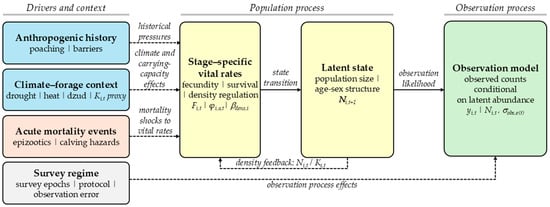
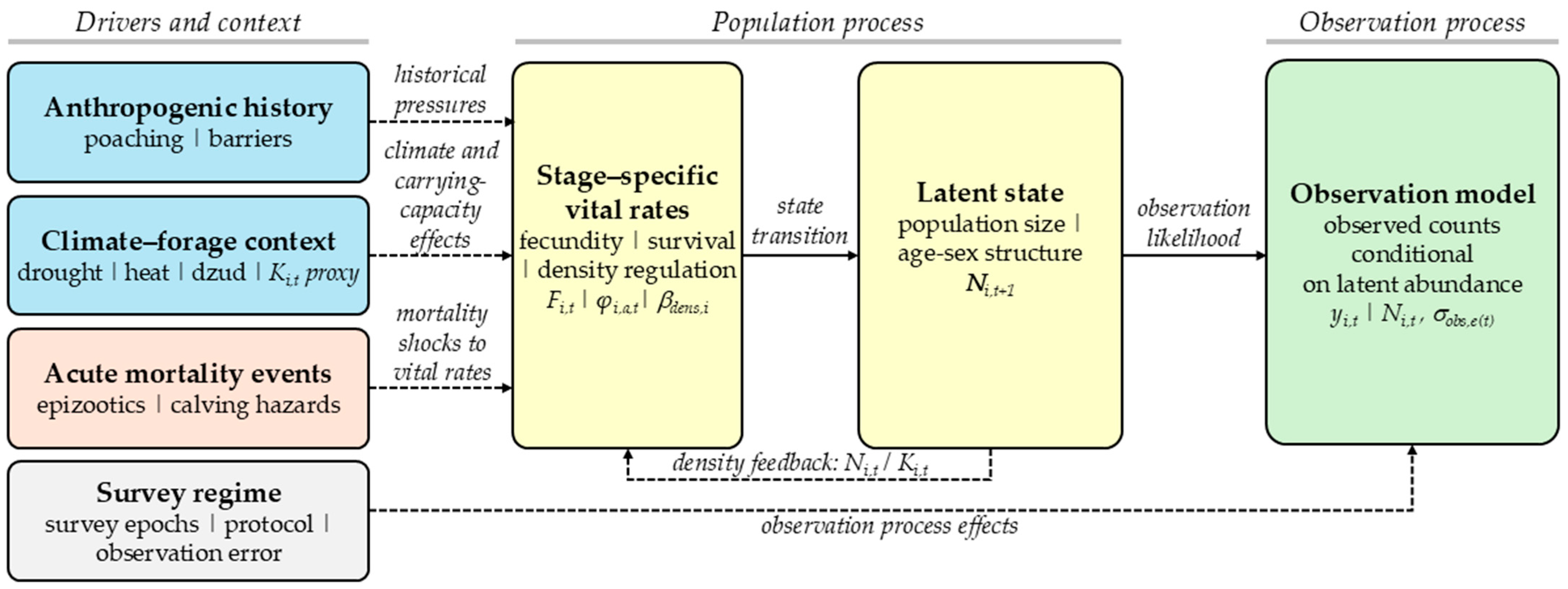
Figure 1 provides the conceptual structure for the stage-structured state-space model and the model-ladder evidence classes. Table 1 lists the corresponding model-family labels, implementation identifiers, and inference status. The ladder defines a sequence of increasingly complex or targeted formulations. Its purpose is not automatic model selection, but the controlled evaluation of structural hypotheses and diagnostic adequacy. The compact model evidence and claim-boundary summary in Appendix A (Table A2) defines the evidence role and permitted manuscript use of each model family.
Figure 1.
Methodological foundation of the saiga stage-structured state-space model and model ladder. Composite framework illustrating the stage-structured state-space model and the model-ladder evidence classes. The ladder separates baseline comparator evidence, sensitivity evidence, development evidence, future validation scaffolds, and blocked decision-facing outputs. Later stages indicate structural development and do not imply operational promotion unless all diagnostic gates are cleared.
A model can be promoted to final inference only if it passes all manuscript gates: maximum R-hat ≤ 1.05; minimum ESS ≥ 400; posterior-predictive coverage ≥ 0.90 for model families where posterior-predictive checks were implemented; no unresolved observed-to-latent mismatch that invalidates the intended claim; and no unsupported management interpretation.
Failure of any hard gate blocks final inference promotion. Such a model may still be scientifically useful as baseline evidence, sensitivity evidence, or negative model-development evidence. This conservative workflow follows standard Bayesian modelling guidance by separating model construction, computation, posterior checking, and claim status rather than treating a fitted model as automatically validated [35,36].
3. Results
3.1. Abundance Phases and Adverse-Period Context
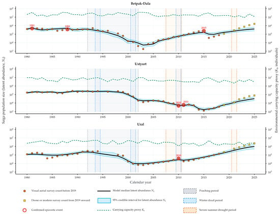
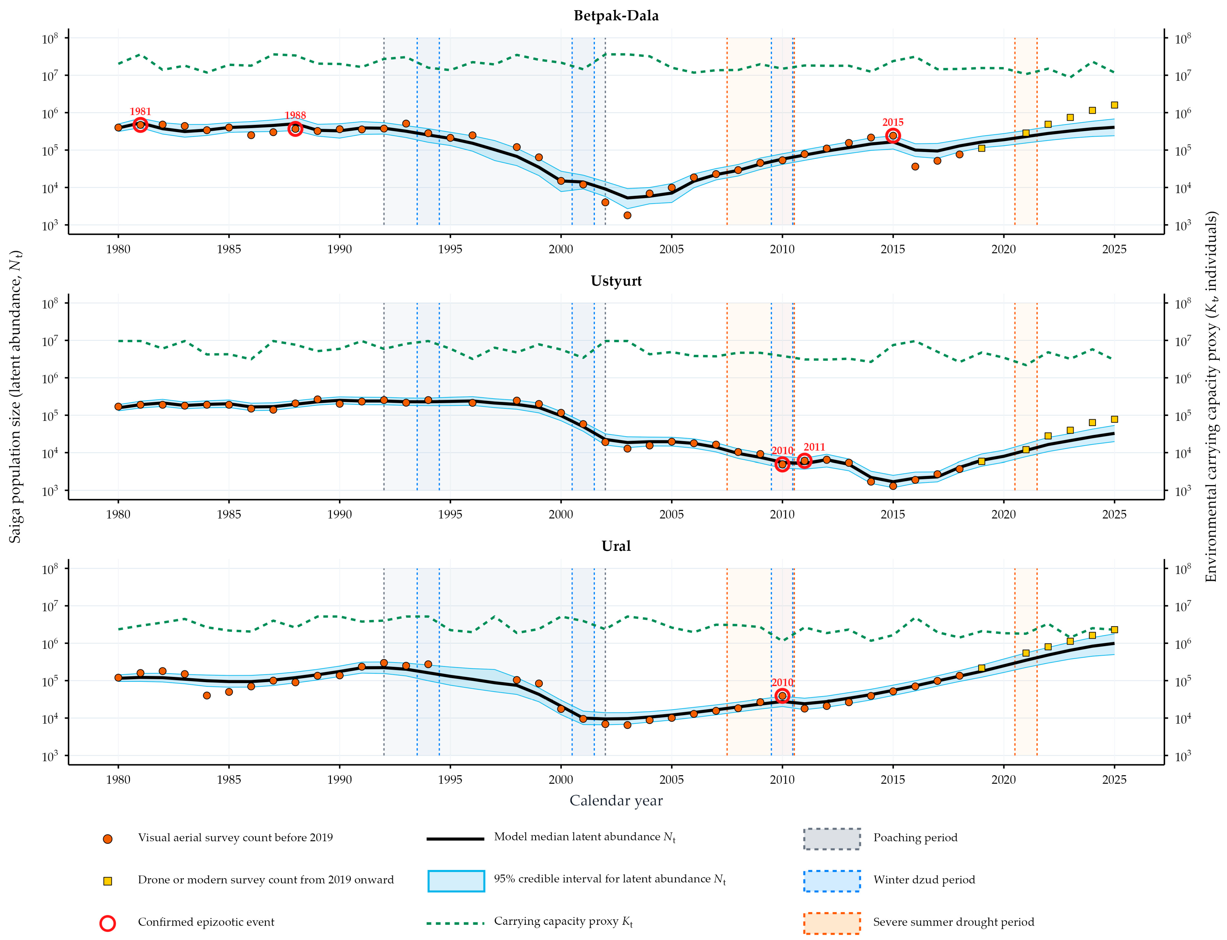
All three populations show a sequence of broad abundance phases: severe historical collapse or low abundance, recovery from the low state, and rapid recent expansion as shown at Figure 2. These phases are not equivalent to a formal regime classification, but they provide a useful biological frame for interpreting the diagnostic model outputs.
Figure 2.
Integrated dynamics: population abundance and carrying capacity proxy across three Kazakhstan saiga populations. Unified population trajectories and environmental capacity profiles for the Betpak-Dala, Ustyurt, and Ural populations. The figure is interpreted as a diagnostic reconstruction and model comparison, not as final post-2020 abundance inference.
The comparatively favourable demographic intervals are those in which the abundance was increasing or remained high without an immediately visible collapse in the count series and without a strong departure from a balanced age–sex structure in the reconstruction. In this manuscript, favourable demographic intervals mean comparatively less constrained periods in the observed reconstruction, not disease-free, density-independent, or management-secure states. The adverse periods are represented by known crisis bands and environmental-stress intervals, including post-Soviet poaching pressure, winter dzud stress, summer drought, and acute mass-mortality epizootics. The model ladder indicates that these adverse periods are central to reconstruction because they can interrupt growth, alter demographic structure, and leave a legacy that simple smooth abundance models cannot reproduce.
The post-2020 period is especially important because the observed counts rise above the abundance levels reproduced by the baseline latent process. This late-series observed-to-latent mismatch is the central empirical diagnostic result of the manuscript and is summarised in Table 2.
Table 2.
Baseline late-series observed-to-latent mismatch in 2025.
3.2. Baseline Observed-to-Latent Mismatch and Current State
These ratios are not corrected abundance estimates. They are diagnostic measures showing that the baseline model family (M0) does not fully capture contemporary recovery dynamics.
The mismatch also limits the interpretation of the current population state. High recent counts show rapid recovery in the observed series, but the current model-family set cannot yet determine whether the populations are near a stable favourable state, temporarily above a static carrying-capacity approximation, or responding rapidly to a short period of favourable environmental and observation conditions. The present evidence therefore does not support treating the current situation as demographically comfortable or regulation-ready.
3.3. Demographic Structure and Population Condition
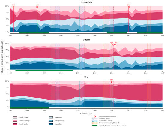
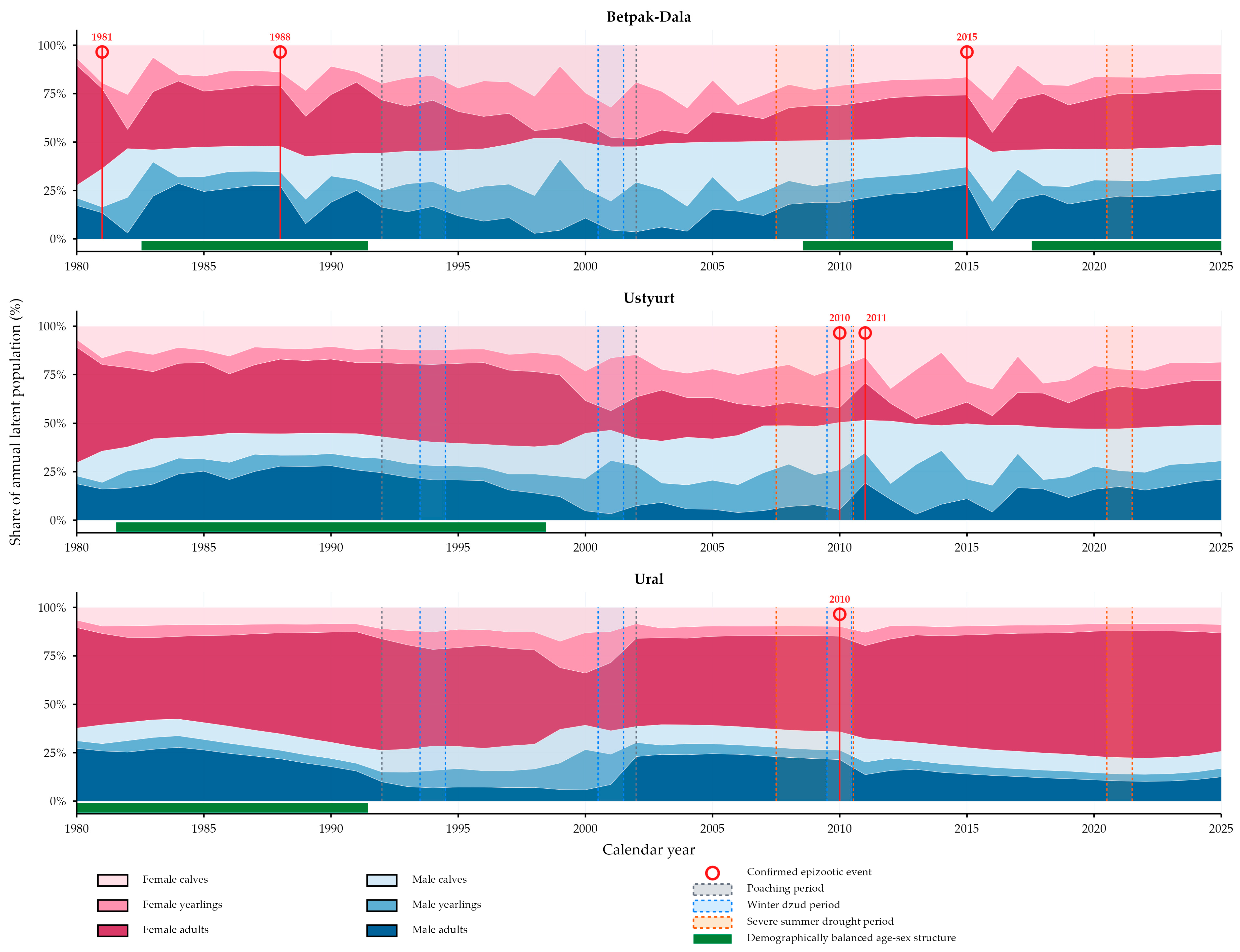
Figure 3 is the main demographic result. It summarises the stage-sex composition and crisis timing in a way that is useful for biological interpretation, including intervals with a demographically balanced age-sex structure, while preserving the diagnostic boundary that baseline demographic parameters are reconstruction summaries rather than final current demographic rates.
Figure 3.
Stage-sex demographic structure and ecosystem crisis timeline. Reconstructed stage-sex composition histories for the three populations, overlaid with crisis bands for post-Soviet poaching, winter dzud stress, summer droughts, and acute mass-mortality epizootics. The figure supports demographic reconstruction and hypothesis refinement, not final management thresholds. Event markers indicate the exogenous event inputs used for survival sensitivity and do not represent independently estimated causal effects.
Population-specific demographic pyramid figures are routed to Appendix A as Figure A1 for Betpak-Dala, Figure A2 for Ustyurt, and Figure A3 for Ural.
The demographic reconstruction supports three cautious population-level interpretations.
Betpak-Dala. The observed data show the largest modern recovery and a strong current count. However, M0 underpredicts the 2025 abundance, and R2 improves the alignment without passing the ESS gate. The population should therefore be interpreted as rapidly recovered but not yet diagnostically resolved. The current high count alone is not sufficient evidence that the population is in a comfortable long-term state.
Ustyurt. The observed data show a severe historical collapse and slower recovery. Although the recent counts are higher than during the lowest period, the population remains the smallest of the three in the modelling dataset and is still sensitive to reporting-version, observation, and process uncertainty. Its current state should be treated as fragile recovery rather than secure abundance.
Ural. The observed data show rapid modern growth and the largest 2025 count. The 2,300,000 value is a Kazakhstan survey-domain report estimate, but the accessible documentation does not provide a comparable decomposition into the direct count, aerial extrapolation, surveyed area, and ground adjustment. The static-K baseline is especially inadequate for this population, and the observed count greatly exceeds the baseline latent median. Because the present model has no movement term and the Ural population is seasonally transboundary, the increase is an increase in the reported abundance series, not evidence that local reproduction and survival have been isolated from redistribution, immigration, boundary changes, or survey-coverage changes. The result supports a rapid expansion in the count series, but not a validated conclusion that the population is safely buffered against future environmental limitation or density feedback.
Across all three populations, the stage-sex and abundance outputs suggest that recent growth may partly reflect a rapid demographic response to favourable conditions after earlier constraints. Because the fitted model-family set has not passed the final gates, the timing, magnitude, and mechanism of any future decline cannot be quantified. Nevertheless, the reconstruction is consistent with the possibility that the abundance could decline in future even without a direct human reduction if the environmental conditions, density feedback, disease risk, forage limitation, or observation-regime conditions shift unfavourably.
3.4. Model Ladder and Sensitivity Diagnostics
The joint-hierarchical model-family path improves the late-series alignment more than the baseline, dynamic-K-only, observation-regime-only, or empirical-prior-pooling families. However, no fitted candidate clears all manuscript gates. Appendix A, Table A2, summarises the evidence role and permitted manuscript use of each model family.
For the strongest development family M4b R2 (sampling-optimised joint-hierarchical development family), the 2025 observed-to-latent ratios decreased to approximately 1.77 for Betpak-Dala, 1.43 for Ustyurt, and 1.49 for Ural. These values indicate an improved late-series alignment relative to M0, but they are not promoted to the final inference because ESS remained below the predefined gate of 400 in all populations. The improvement in late-series alignment is a reconstruction-level result. It does not imply that the model has identified the current population-specific survival, fecundity, density feedback, or movement rates, because the minimum ESS and other promotion gates remain unmet. Representative low-ESS nodes involved the fecundity hierarchy and climate-linked adult-survival terms; the examples are reported in Supplementary Table S4.
3.5. Forecasts and Risk Products
Forecast fans, scenario surfaces, and risk heatmaps are excluded from the main results. They are exploratory proxy outputs derived from non-final model components or post-processing layers. They do not support management-ready conclusions, harvest thresholds, removal quotas, population-regulation rules, or risk rankings.
4. Discussion
The analysis supports a conservative but scientifically useful conclusion. The current analysis workflow and model-family set provide a reproducible, climate-aware, sex- and stage-structured reconstruction of three saiga population trajectories. They also show that the baseline structure fails to capture the magnitude of the recent recovery, and that plausible extensions improve but do not fully solve the problem.
This negative result is scientifically valuable. It identifies the boundary between historical reconstruction and final demographic inference. It also shows that post-2020 saiga dynamics require either stronger observation-process information, the better modelling of contemporary demographic regimes, an improved carrying-capacity structure, the explicit treatment of population closure and immigration, or a better-sampling implementation of the joint-hierarchical model family.
The reconstructed trajectories also clarify why a simple interpretation of recent counts is risky. Periods with a comparatively favourable demographic structure in the count series are best understood as intervals of demographic release or lower visible constraint, not as proof that the populations are at a secure equilibrium. Conversely, adverse periods can affect the population through multiple routes: direct mortality, reduced recruitment, an altered stage-sex structure, a changed detection context, and delayed recovery from previous depletion. These mechanisms are consistent with the crisis bands and demographic reconstruction, but the present model-family set cannot yet partition their causal contributions with final precision.
The main finding is therefore not a single accepted final model family, but a consistent diagnostic pattern across the model ladder. Observed trajectories show collapse and recovery across all three populations, and the baseline family (M0) provides an auditable reconstruction of that broad history. At the same time, late-series underprediction is systematic, recent high counts do not by themselves prove a comfortable demographic state, and single-mechanism fixes remain insufficient. True joint-hierarchical pooling improves alignment but remains diagnostically incomplete, while the R2 development family is the strongest current sensitivity candidate rather than a final model family.
The current analysis reconstructs the broad changes in the reported abundance, but it does not yet provide reliable population-specific vital rates for the present period. In particular, it cannot separate local reproduction and survival from changes in survey coverage, observation conditions, composite aerial/ground adjustments, spatial redistribution, or unmeasured environmental constraints. The systematic late-series mismatch therefore indicates that the current ecological covariate set is incomplete; future work should prioritise survey coverage and detection, spatial redistribution and transboundary movement, pathogen and outbreak intensity, age- and sex-specific recruitment, and forage and density-dependence data. The outputs should therefore not be used for policy-grade forecasts, harvest or removal thresholds, management-ready risk maps, or as a validated final population model.
This limitation is especially important for any discussion of population regulation. The current analysis does not provide a sufficiently precise or validated picture for numerical recommendations about reducing, harvesting, or otherwise regulating abundance. The populations are not shown to be in a comfortable state simply because the recent counts are high. The recent increase may represent a rapid response to favourable environmental conditions, demographic release after previous constraints, changes in observation context, or a combination of these processes. If environmental conditions become less favourable, if density feedback strengthens, or if disease and forage constraints re-emerge, abundance could decline even without direct human reduction. The present model can identify this as a plausible risk, but it cannot yet estimate the timing or size of such a decline.
The current analysis supports a qualitative and precautionary conservation interpretation only: continued monitoring, stronger observation metadata, pathogen surveillance, climate and forage data integration, and transboundary coordination. Quantitative offtake, harvest thresholds, removal recommendations, or regulation rules require a validated future model that clears all diagnostic and posterior-predictive gates.
The next step is to test the same ecological model on simulated and improved observations before interpreting it as a final population model. The first stage is targeted JAGS stabilisation using M4b R3 (targeted JAGS validation scaffold) and, if necessary, benchmarking an equivalent NIMBLE implementation against the M4b R2 reference fit. NIMBLE may allow samplers and block updates that are better suited to the strong correlations among latent abundance, survival, fecundity, and density feedback, but it is not assumed to solve the problem automatically. Only a model that recovers known simulated histories and passes all predefined diagnostic and observed-to-latent mismatch gates should support final inference [37].
5. Conclusions
This study should be interpreted as a transparent reconstruction and sensitivity audit, not as a final demographic assessment. The scientific value lies in the reproducible model ladder, explicit diagnostic gates, observed-to-latent mismatch, demographic context, and negative evidence showing that plausible structural fixes remain insufficient for the final inference. The current evidence supports precautionary monitoring and model development, but not numerical regulation, harvest, removal, or risk-threshold recommendations.
The most important conclusion is conditional: hierarchical pooling and reparameterisation are promising, but not yet diagnostically complete. With further validation, they may provide a useful insight into the population structure and demographic processes, help distinguish shared from population-specific dynamics, and guide future modelling and field studies. At present, however, they should be treated as development evidence rather than as a validated basis for the final demographic inference.
Supplementary Materials
The following supporting information can be downloaded at: https://www.mdpi.com/article/10.3390/ecologies7030082/s1, Table S1: Variable dictionary for Supplementary Dataset S1; Table S2: Complete harmonised annual count series used in modelling, including missing-count years, 1980–2025; Table S3: 2025 count provenance and model handling; Table S4: Representative low-ESS diagnostics for M4b R2; Table S5: Computational implementation and reproducibility map; Table S6: Structure of Supplementary Code S1; Listings S1–S3: Essential M0 and M4b R2 model-code excerpts and minimal execution commands; Supplementary Dataset S1: machine-readable harmonised annual counts, model inputs, observation metadata, README, and manifest; and Supplementary Code S1: a focused isolated M0/M4b R2 reproduction package containing executable R code, local input copies, priors, frozen evidence maps, README, manifest, and verification record.
Author Contributions
I.G.F.: conceptualization, data curation, formal analysis, investigation, methodology, software, validation, visualization, writing—original draft, and writing—review and editing. A.A.G.: supervision, investigation, data curation, resources, and compilation and provenance clarification of the harmonised long-term annual saiga count series. A.K.: investigation, data curation, and validation. Y.T.: project administration, and supervision. All authors have read and agreed to the published version of the manuscript.
Funding
This research was supported by the Forestry and Wildlife Committee of the Ministry of Ecology and Natural Resources of the Republic of Kazakhstan (Grant No. BR23591114), “Development of a system for sustainable use of the Betpak-Dala and Ustyurt saiga populations”.
Institutional Review Board Statement
Not applicable. This study used compiled annual monitoring records and did not involve the experimental manipulation of animals.
Informed Consent Statement
Not applicable.
Data Availability Statement
The non-restricted harmonised annual count and exact model-input tables are provided in machine-readable form as Supplementary Dataset S1. The complete annual count series is also presented in human-readable form in Supplementary Table S2. Supplementary Dataset S1 includes units, missingness indicators, observation-method and observation-error classes, event indicators, derived covariates, and provenance documentation. The focused executable source package for M0 and M4b R2 is provided as Supplementary Code S1. Production scripts for M2, M3, M4, M4b, M4b R1, and M4b R3 are not included; these model families are represented only by explicitly labelled frozen taxonomy and diagnostic evidence. The historical series was harmonised from the published literature, institutional reports, Kazakhstan state monitoring summaries, and public annual estimates; it is not a single primary survey dataset. The underlying institutional records and restricted monitoring materials remain subject to permission from the data holders. The technical model assumptions are described in Section 2.2, Section 2.3 and Section 2.4 and Section 2.6; the computational versions, execution order, and package structure are documented in Supplementary Table S5, Section S5.1 of the Supplementary Materials, and Supplementary Table S6, respectively.
Acknowledgments
The authors thank the Institute of Zoology, Republic of Kazakhstan, Almaty, for the institutional support. We also acknowledge the field teams and institutions involved in long-term saiga monitoring and aerial surveys, including the Association for the Conservation of Biodiversity of Kazakhstan (ACBK), Okhotzooprom, territorial wildlife inspection bodies, and protected-area staff.
Conflicts of Interest
The authors declare no conflicts of interest.
Abbreviations
The following abbreviations are used in this manuscript:
| ACBK | Association for the Conservation of Biodiversity of Kazakhstan |
| ERA5-Land | ECMWF Reanalysis v5-Land |
| ESS | Effective sample size |
| IPM | Integrated population model |
| JAGS | Just Another Gibbs Sampler |
| K | Carrying capacity |
| LAI | Leaf area index |
| MCMC | Markov chain Monte Carlo |
| NIMBLE | Numerical Inference for statistical Models using Bayesian and Likelihood Estimation |
| R-hat | Potential scale reduction factor |
Appendix A
Appendix A contains the population-specific demographic pyramid figures (Figure A1, Figure A2 and Figure A3), the compact covariate dictionary (Table A1), and the model evidence and claim-boundary summary (Table A2). The complete annual count series and computational materials are provided separately in the Supplementary Materials.
Figure A1.
Betpak-Dala population-specific demographic pyramid. Annual medians and uncertainty intervals are shown by stage and sex, with females plotted to the right and males to the left. Filled bars show stage-sex medians, box intervals and whiskers show posterior uncertainty, and event symbols mark crisis and monitoring context.
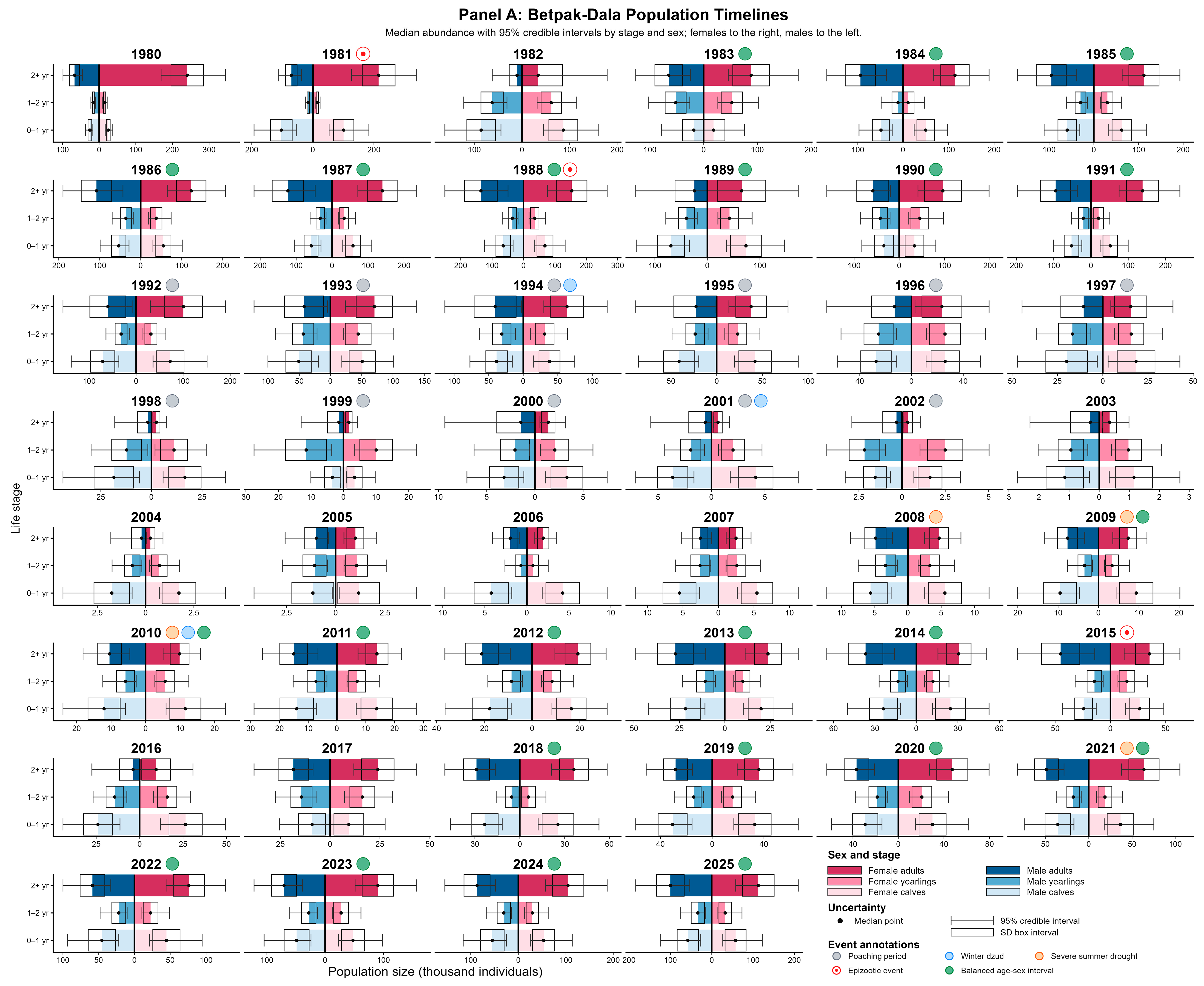
Figure A2.
Ustyurt population-specific demographic pyramid. Annotations follow Figure A1.
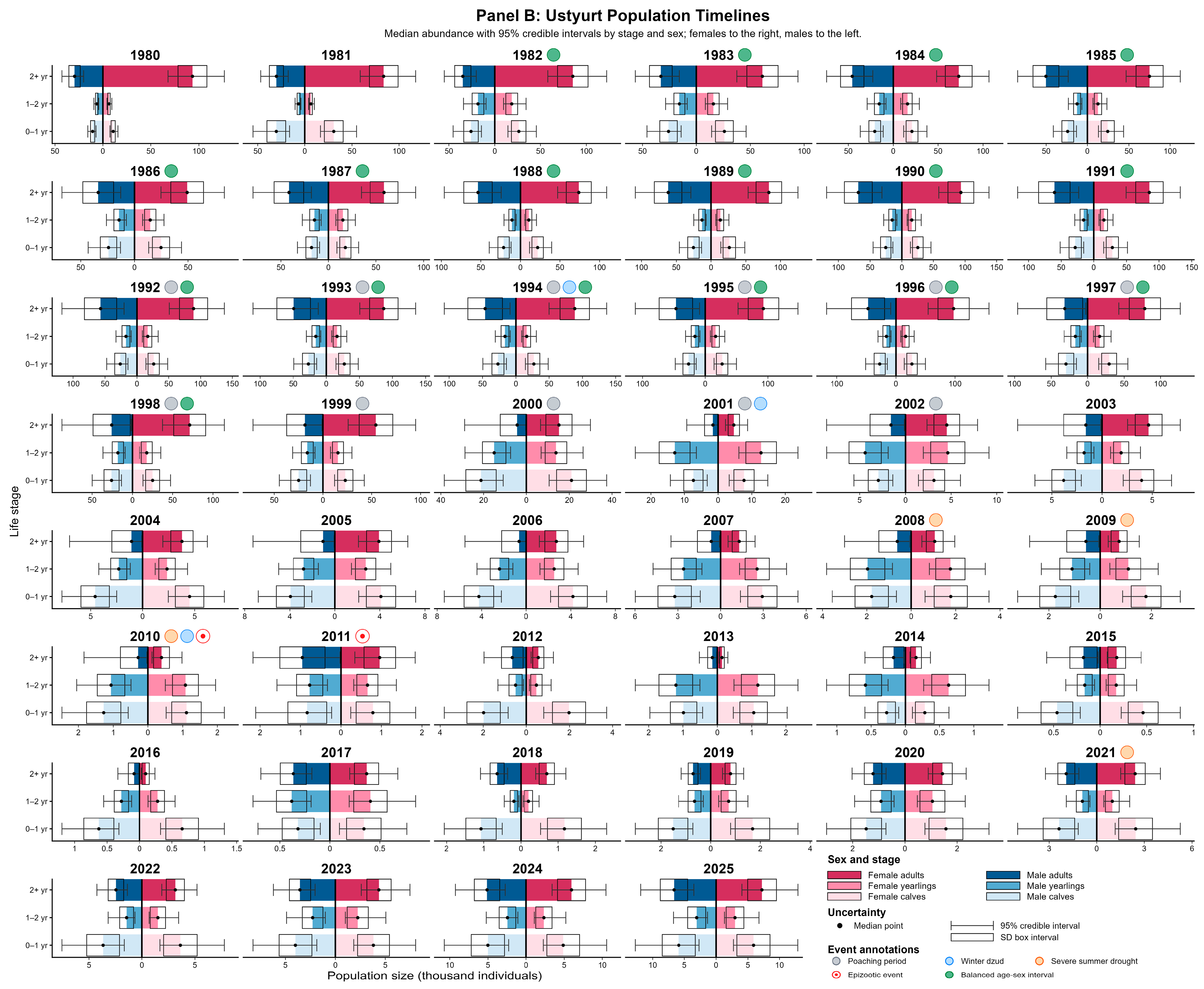
Figure A3.
Ural population-specific demographic pyramid. Annotations follow Figure A1.
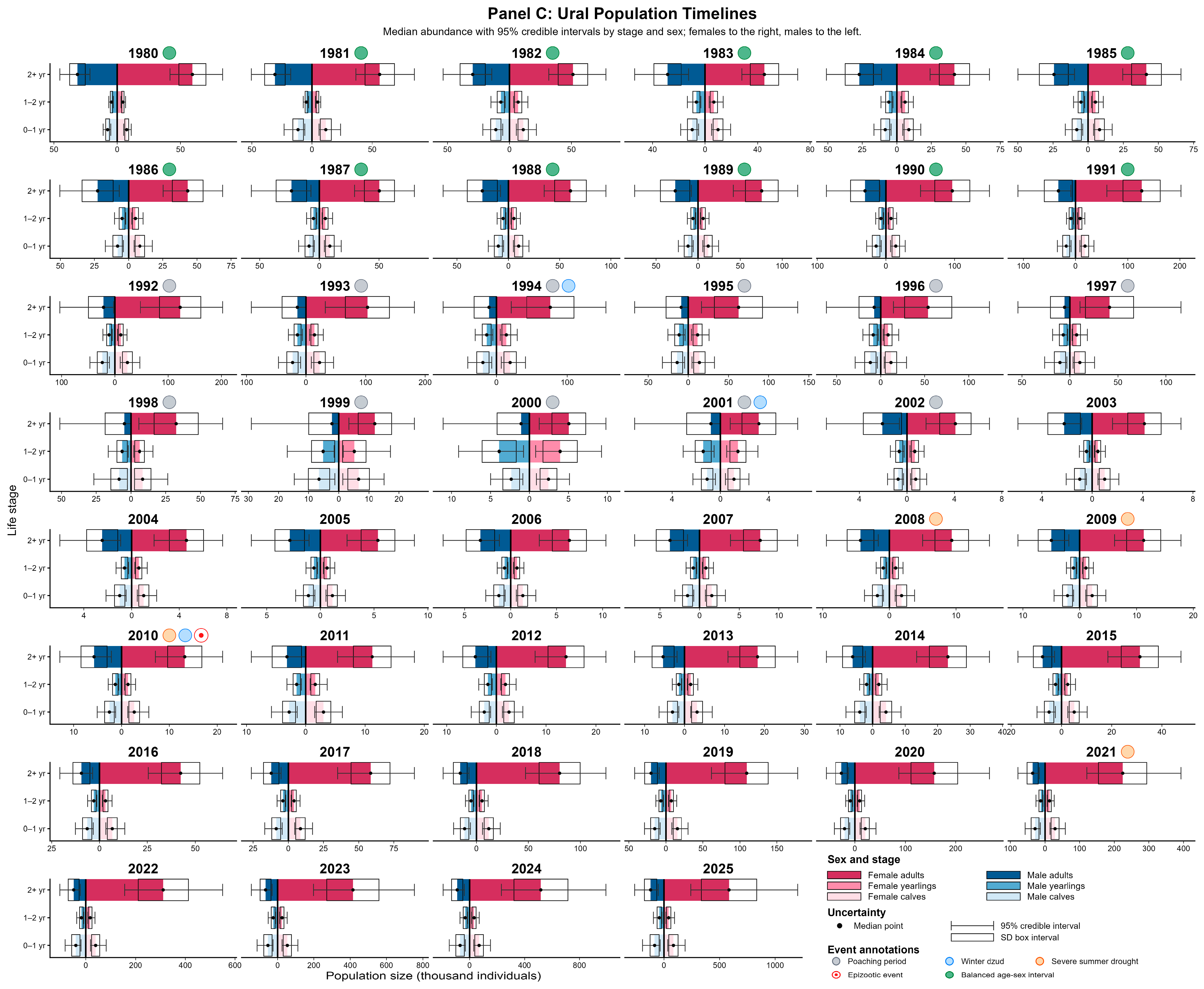
Table A1.
Compact covariate dictionary. These covariates provide environmental, forage, and event context for the model ladder. They are not interpreted as final causal effects unless a successor model clears the manuscript diagnostic and posterior-predictive gates.
Table A2.
Compact model evidence and claim-boundary summary. Models that fail a hard diagnostic gate may be useful as baseline, sensitivity, negative, or development evidence, but they are not promoted to final IPM inference or decision-facing outputs.
References
- Bekenov, A.B.; Grachev, I.A.; Milner-Gulland, E.J. The ecology and management of the Saiga antelope in Kazakhstan. Mammal. Rev. 1998, 28, 1–52. [Google Scholar] [CrossRef] [Scilit]
- Milner-Gulland, E.J.; Kholodova, M.V.; Bekenov, A.; Bukreeva, O.M.; Grachev, I.A.; Amgalan, L.; Lushchekina, A.A. Dramatic declines in saiga antelope populations. Oryx 2001, 35, 340–345. [Google Scholar] [CrossRef] [Scilit][Green Version]
- Kock, R.A.; Orynbayev, M.; Robinson, S.; Zuther, S.; Singh, N.J.; Beauvais, W.; Morgan, E.R.; Kerimbayev, A.; Khomenko, S.; Martineau, H.M.; et al. Saigas on the brink: Multidisciplinary analysis of the factors influencing mass mortality events. Sci. Adv. 2018, 4, eaao2314. [Google Scholar] [CrossRef] [Scilit] [PubMed]
- IUCN SSC Antelope Specialist Group. Saiga tatarica. The IUCN Red List of Threatened Species 2023, e.T19832A233712210. Available online: https://www.iucnredlist.org/species/19832/233712210 (accessed on 8 August 2026).
- Convention on Migratory Species (CMS). Medium-Term International Work Programme for the Saiga Antelope (2025–2030). UNEP/CMS/Saiga/MOS5/Outcome 2/Rev.1, 25 September 2025. 2025. Available online: https://www.cms.int/document/medium-term-international-work-programme-saiga-antelope-2025-2030 (accessed on 8 August 2026).
- Kühl, A.; Mysterud, A.; Grachev, I.A.; Bekenov, A.B.; Ubushaev, B.S.; Lushchekina, A.A.; Milner-Gulland, E.J. Monitoring population productivity in the saiga antelope. Anim. Conserv. 2009, 12, 355–363. [Google Scholar] [CrossRef] [Scilit]
- McConville, A.J.; Grachev, I.A.; Keane, A.; Coulson, T.; Bekenov, A.B.; Milner-Gulland, E.J. Reconstructing the observation process to correct for changing detection probability of a critically endangered species. Endanger. Species Res. 2009, 6, 231–237. [Google Scholar] [CrossRef]
- Singh, N.J.; Milner-Gulland, E.J. Conserving a moving target: Planning protection for a migratory species as its distribution changes. J. Appl. Ecol. 2011, 48, 35–46. [Google Scholar] [CrossRef] [Scilit]
- Besbeas, P.; Freeman, S.N.; Morgan, B.J.T.; Catchpole, E.A. Integrating mark-recapture-recovery and census data to estimate animal abundance and demographic parameters. Biometrics 2002, 58, 540–547. [Google Scholar] [CrossRef] [Scilit] [PubMed]
- Schaub, M.; Abadi, F. Integrated population models: A novel analysis framework for deeper insights into population dynamics. J. Ornithol. 2011, 152, S227–S237. [Google Scholar] [CrossRef] [Scilit]
- Arnold, T.W.; Clark, R.G.; Koons, D.N.; Schaub, M. Integrated population models facilitate ecological understanding and improved management decisions. J. Wildl. Manag. 2018, 82, 266–274. [Google Scholar] [CrossRef] [Scilit]
- Riecke, T.V.; Williams, P.J.; Behnke, T.L.; Gibson, D.; Leach, A.G.; Sedinger, B.S.; Street, P.A.; Sedinger, J.S. Integrated population models: Model assumptions and inference. Methods Ecol. Evol. 2019, 10, 1072–1082. [Google Scholar] [CrossRef] [Scilit]
- Schaub, M.; Kéry, M. Integrated Population Models: Theory and Ecological Applications with R and JAGS; Academic Press: London, UK, 2021. [Google Scholar]
- Regan, H.M.; Colyvan, M.; Burgman, M.A. A taxonomy and treatment of uncertainty for ecology and conservation biology. Ecol. Appl. 2002, 12, 618–628. [Google Scholar] [CrossRef]
- Runge, M.C.; Converse, S.J.; Lyons, J.E. Which uncertainty? Using expert elicitation and expected value of information to design an adaptive program. Biol. Conserv. 2011, 144, 1214–1223. [Google Scholar] [CrossRef] [Scilit]
- Addison, P.F.E.; Rumpff, L.; Bau, S.S.; Carey, J.M.; Chee, Y.E.; Jarrad, F.C.; McBride, M.F.; Burgman, M.A. Practical solutions for making models indispensable in conservation decision-making. Divers. Distrib. 2013, 19, 490–502. [Google Scholar] [CrossRef] [Scilit]
- Milner-Gulland, E.J.; Shea, K. Embracing uncertainty in applied ecology. J. Appl. Ecol. 2017, 54, 2063–2068. [Google Scholar] [CrossRef] [Scilit] [PubMed]
- Gabry, J.; Simpson, D.; Vehtari, A.; Betancourt, M.; Gelman, A. Visualization in Bayesian workflow. J. R. Stat. Soc. Ser. A 2019, 182, 389–402. [Google Scholar] [CrossRef] [Scilit]
- Gelman, A.; Goodrich, B.; Gabry, J.; Vehtari, A. R-squared for Bayesian regression models. Am. Stat. 2019, 73, 307–309. [Google Scholar] [CrossRef] [Scilit]
- Vehtari, A.; Gelman, A.; Simpson, D.; Carpenter, B.; Bürkner, P.-C. Rank-normalization, folding, and localization: An improved R-hat for assessing convergence of MCMC (with discussion). Bayesian Anal. 2021, 16, 667–718. [Google Scholar] [CrossRef] [Scilit]
- Institute of Zoology. Development of a System for Conservation and Sustainable Use of the Betpak-Dala and Ustyurt Saiga Populations in Kazakhstan; Final research report; Institute of Zoology: Almaty, Kazakhstan, 2025; 327p, (In Russian and Kazakh). [Google Scholar]
- Muñoz-Sabater, J.; Dutra, E.; Agustí-Panareda, A.; Albergel, C.; Arduini, G.; Balsamo, G.; Boussetta, S.; Choulga, M.; Harrigan, S.; Hersbach, H.; et al. ERA5-Land: A state-of-the-art global reanalysis dataset for land applications. Earth Syst. Sci. Data 2021, 13, 4349–4383. [Google Scholar] [CrossRef] [Scilit]
- R Core Team. R: A Language and Environment for Statistical Computing; R Foundation for Statistical Computing: Vienna, Austria, 2026; Available online: https://www.R-project.org/ (accessed on 8 August 2026).
- Plummer, M. JAGS: A program for analysis of Bayesian graphical models using Gibbs sampling. In Proceedings of the 3rd International Workshop on Distributed Statistical Computing, Vienna, Austria; Hornik, K., Leisch, F., Zeileis, A., Eds.; Technische Universität Wien: Vienna, Austria, 2003; Available online: https://www.r-project.org/conferences/DSC-2003/Proceedings/Plummer.pdf (accessed on 8 August 2026).
- Plummer, M. rjags: Bayesian Graphical Models Using MCMC, R package version 4.17; R Foundation for Statistical Computing: Vienna, Austria, 2025. [CrossRef] [Scilit]
- Plummer, M.; Best, N.; Cowles, K.; Vines, K. CODA: Convergence diagnosis and output analysis for MCMC. R News 2006, 6, 7–11. [Google Scholar]
- Wickham, H.; Vaughan, D.; Girlich, M. tidyr: Tidy Messy Data, R package version 1.3.2; R Foundation for Statistical Computing: Vienna, Austria, 2025. [CrossRef] [Scilit]
- Wickham, H.; François, R.; Henry, L.; Müller, K.; Vaughan, D. dplyr: A Grammar of Data Manipulation, R package version 1.2.1; R Foundation for Statistical Computing: Vienna, Austria, 2026. [CrossRef] [Scilit]
- Wickham, H.; Hester, J.; Bryan, J. readr: Read Rectangular Text Data, R package version 2.2.0; R Foundation for Statistical Computing: Vienna, Austria, 2026. [CrossRef] [Scilit]
- Müller, K.; Wickham, H. tibble: Simple Data Frames, R package version 3.3.1; R Foundation for Statistical Computing: Vienna, Austria, 2026. [CrossRef] [Scilit]
- Wickham, H.; Henry, L. purrr: Functional Programming Tools, R package version 1.2.2; R Foundation for Statistical Computing: Vienna, Austria, 2026. [CrossRef] [Scilit]
- Wickham, H. ggplot2: Elegant Graphics for Data Analysis; Springer: New York, NY, USA, 2016. [Google Scholar] [CrossRef] [Scilit]
- Pedersen, T.L. patchwork: The Composer of Plots, R package version 1.3.2; R Foundation for Statistical Computing: Vienna, Austria, 2025. [CrossRef] [Scilit]
- Pedersen, T.L.; Shemanarev, M. ragg: Graphic Devices Based on AGG, R package version 1.5.2; R Foundation for Statistical Computing: Vienna, Austria, 2026. [CrossRef] [Scilit]
- Gelman, A.; Carlin, J.B.; Stern, H.S.; Dunson, D.B.; Vehtari, A.; Rubin, D.B. Bayesian Data Analysis, 3rd ed.; Chapman and Hall/CRC: Boca Raton, FL, USA, 2013. [Google Scholar] [CrossRef] [Scilit]
- Talts, S.; Betancourt, M.; Simpson, D.; Vehtari, A.; Gelman, A. Validating Bayesian inference algorithms with simulation-based calibration. arXiv 2018, arXiv:1804.06788. [Google Scholar] [CrossRef] [Scilit]
- de Valpine, P.; Turek, D.; Paciorek, C.J.; Anderson-Bergman, C.; Temple Lang, D.; Bodik, R. Programming with models: Writing statistical algorithms for general model structures with NIMBLE. J. Comput. Graph. Stat. 2017, 26, 403–417. [Google Scholar] [CrossRef] [Scilit]

Disclaimer/Publisher’s Note: The statements, opinions and data contained in all publications are solely those of the individual author(s) and contributor(s) and not of MDPI and/or the editor(s). MDPI and/or the editor(s) disclaim responsibility for any injury to people or property resulting from any ideas, methods, instructions or products referred to in the content. |
© 2026 by the authors. Licensee MDPI, Basel, Switzerland. This article is an open access article distributed under the terms and conditions of the Creative Commons Attribution (CC BY) license.