Closed-Loop Learning-Based PID Tuning for DC Motor Actuators Using Experimental Data

Abstract

This paper addresses experimental PID tuning for DC motor actuators when an accurate plant model is unavailable or impractical to obtain. Controller tuning is formulated as a constrained closed-loop optimization process in which each PID gain set is deployed on the physical system, produces an experimental dataset, and is evaluated through a performance index. The objective function combines tracking error, control effort, and control-signal variation, while penalty terms identify and penalize actuator saturation, excessive overshoot, settling-time violations, steady-state error, and divergent responses. Candidate controllers are generated using a constrained Gaussian Cross-Entropy Method and evaluated directly on the physical actuator. The proposed host-embedded architecture separates two computational time scales: PID execution, encoder processing, and data acquisition are performed in real time on the embedded platform, whereas population sampling, candidate ranking, and distribution updates are executed on the host computer between experiments. Within the reported experimental campaign, the sampling distribution progressively concentrates toward gain regions associated with lower closed-loop cost under the prescribed admissibility criteria. The resulting framework provides a structured and traceable procedure for physical controller deployment, data acquisition, constrained performance evaluation, and episodic PID retuning without explicit plant identification. The reported results demonstrate the feasibility of the architecture on the considered platform, without implying comparative superiority, run-to-run statistical convergence, or analytical closed-loop stability.

1. Introduction

Proportional–Integral–Derivative (PID) controllers remain widely used in industrial and embedded control systems because of their simple structure, low computational cost, and compatibility with resource-constrained hardware [1,2]. Nevertheless, selecting the proportional, integral, and derivative gains remains a nontrivial problem. Closed-loop performance can be affected by nonlinear friction, actuator saturation, measurement noise, uncertain parameters, discrete sampling, quantization, and communication constraints, particularly when the controller is implemented on a low-cost physical platform.

Model-based tuning methods provide systematic design procedures when an adequate plant representation is available. Internal Model Control tuning relates controller parameters to an identified process model and prescribed robustness requirements [3]. Relay-based and reduced-order approaches can also derive PID gains from simplified process dynamics [4]. However, the resulting controller performance depends on the correspondence between the assumed model and the actual plant. Obtaining a sufficiently accurate model may require dedicated excitation experiments, structural assumptions, and parameter-estimation procedures. These requirements can become restrictive in embedded motor-control applications, where nonlinearities, unknown loads, encoder quantization, actuator limitations, and hardware-dependent effects may reduce the validity of the identified representation [5,6].

Data-driven controller tuning was developed to reduce the dependence on explicit plant identification. Iterative Feedback Tuning estimates performance gradients from closed-loop experiments and updates the controller directly from measured responses [7]. Virtual Reference Feedback Tuning constructs a controller from input–output data and a desired reference model without identifying a parametric plant representation [8]. Convex data-driven robust control and model-free adaptive formulations have further shown that controller synthesis can be based on measured trajectories rather than on a predetermined dynamic model [9,10]. These methods differ in their data requirements, controller parameterizations, auxiliary assumptions, and available stability or robustness guarantees.

Recent research has extended direct PID tuning toward online, one-shot, constrained, and experimentally optimized formulations. Zhu et al. [11] developed an online auto-tuning method for minimum-variance PID control using operational data. Yonezawa et al. [12] proposed a one-shot data-driven design for fractional-order PID controllers based on a fictitious reference signal, thereby reducing the required number of experiments. Liu et al. [13] formulated a data-driven optimal PID tuning method for nonlinear systems while incorporating closed-loop performance and analytical stability conditions. These contributions demonstrate that tuning PID controllers from measured data is an established research direction. Consequently, the use of experimental data without explicit plant identification does not, by itself, constitute the principal contribution of the present work.

Repeated interaction with the controlled system provides an alternative mechanism for controller improvement. Iterative Learning Control updates the control action from errors observed over repeated executions of the same task [14]. Extremum-seeking methods optimize a measurable performance index without requiring an explicit model and have been applied directly to PID tuning [15,16,17]. Reinforcement learning similarly formulates controller improvement through system interaction and performance feedback [18]. Although these approaches provide important foundations for model-free learning, their implementation on physical embedded systems requires careful consideration of excitation, experimental duration, computational allocation, safety constraints, and the distinction between real-time feedback control and parameter adaptation.

Stochastic and population-based algorithms provide additional mechanisms for exploring nonconvex controller-parameter spaces. Evolutionary algorithms have been extensively investigated in control engineering [19], while simultaneous perturbation methods provide gradient-free optimization with a reduced number of objective-function evaluations [20]. Swarm-inspired methods have also been applied to nonlinear and multimodal controller-tuning problems [21]. Experimental motor-control implementations have combined genetic optimization with fuzzy PID structures on digital signal processors [22]. More recently, Massoud and Libby [23] compared evolutionary PID tuning algorithms through simulation and physical experiments on a pneumatic soft robotic system. Saat et al. [24] incorporated a safe experimentation dynamics algorithm into a data-driven intelligent PID structure and evaluated the stochastic variability of the optimization process. These studies demonstrate the applicability of population-based tuning while also identifying practical trade-offs involving the number of physical experiments, campaign duration, stochastic repeatability, constraint handling, and computational distribution.

The Cross-Entropy Method (CEM) is an adaptive stochastic optimization technique that updates a sampling distribution using the best-performing candidates in each population [25,26]. Its use in the present work is not claimed as a new optimization algorithm. Instead, CEM provides the sampling, ranking, and distribution-update mechanism required to implement the proposed experimental architecture. The contribution therefore does not arise from PID control, physical experimentation, or stochastic optimization considered independently.

Existing studies provide mature solutions for data-driven tuning, iterative optimization, and population-based controller search. However, these elements are often described separately, while less attention is given to the end-to-end implementation of a host-embedded process in which every sampled controller is physically deployed, the requested and applied experimental conditions are recorded, synchronized closed-loop signals are returned through a structured communication protocol, and performance and admissibility criteria are evaluated within the same optimization map. The research gap addressed in this study therefore concerns the formal integration and traceability of the complete experimental learning process under embedded implementation constraints, rather than the introduction of another standalone PID optimization algorithm.

Accordingly, the objective of this study is to formulate and experimentally examine a closed-loop learning architecture for PID tuning in which the controller gains constitute the decision variables,

$$K={\left[\begin{array}{ccc}{K}_p& K_i& K_d\end{array}\right]}^T,$$

(1)

and every candidate controller produces a physical closed-loop experiment through the mapping

$$K⟼E\left(K\right)⟼J\left(K\right).$$

(2)

Here, $E\left(K\right)$ denotes the dataset acquired after deploying K on the embedded motor system, whereas $J\left(K\right)$ combines tracking error, control effort, control-signal variation, and penalty terms associated with experimentally defined inadmissibility criteria. This formulation establishes a direct correspondence among the optimization variables, the physical experiment, the measured signals, and the resulting performance evaluation.

The penalty terms are used to reject or discourage experimentally undesirable responses, including excessive saturation, overshoot, settling-time violations, steady-state error, and divergence. These terms constitute operational safeguards for the experimental search and should not be interpreted as analytical closed-loop stability conditions. Because no parametric plant model is employed, the present study does not derive a Lyapunov certificate, a robust-stability margin, or a general stability guarantee for arbitrary PID gains and operating conditions.

The proposed architecture separates two computational time scales. The PID controller is executed deterministically on the embedded processor at a fixed sampling period, whereas population sampling, candidate ranking, cost evaluation, and distribution adaptation are performed on the host computer between experiments. Consequently, the method is intended for experimental commissioning or episodic retuning and is not presented as a gain-adaptation law operating within each real-time control sample. This computational partition keeps the stochastic optimizer outside the embedded feedback period while preserving direct interaction with the physical actuator.

The main contributions of this study are summarized as follows:

• An end-to-end closed-loop experimental formulation that explicitly connects the PID gain vector, the physical experiment, the acquired dataset, and the constrained performance index through the mapping

  $$K⟼E\left(K\right)⟼J\left(K\right).$$
• A host-embedded architecture that separates deterministic real-time PID execution from episodic stochastic optimization, allocating population storage, candidate ranking, and distribution updates to the host computer.
• A traceable experimental protocol that records the requested controller parameters, the values confirmed by the embedded system, the reference and measured response, the controller command, and the termination state associated with every candidate evaluation.
• A unified experimental evaluation function that combines tracking error, control effort, and control-signal variation with explicit penalties for actuator saturation, excessive overshoot, settling-time violations, steady-state error, and divergent responses.
• A physical implementation on a DC geared-motor actuator that demonstrates the complete execution of the proposed learning cycle under discrete sampling, encoder quantization, actuator saturation, serial communication, and embedded hardware constraints.

The significance of the framework lies in the structured and traceable integration of controller deployment, data acquisition, constrained evaluation, and stochastic distribution updating. The contribution is therefore methodological and architectural. It does not rely on claiming novelty for CEM or experimental PID tuning in isolation.

The experimental results presented in this study correspond to one complete stochastic optimization campaign. They characterize the internal evolution of the sampling distribution and the performance obtained on the considered physical platform, but they do not establish run-to-run statistical convergence. Furthermore, no alternative model-free tuning algorithm is implemented on the same testbed. Therefore, the study does not claim superiority in convergence speed, control performance, or number of physical experiments. These limitations delimit the scope of the reported results and motivate repeated campaigns and controlled comparative experiments as subsequent research directions.

The remainder of this article is organized as follows. Section 2 presents the mathematical formulation of the closed-loop experimental PID tuning problem, including the experimental mapping, discrete-time PID parameterization, constrained performance index, and Gaussian Cross-Entropy Method. Section 3 describes the physical DC motor platform, embedded feedback architecture, operating conditions, serial communication protocol, and experimental dataset construction. Section 4 details the host-embedded algorithmic implementation, distinguishing the host-side optimization procedures from the real-time embedded control and acquisition tasks. Section 5 specifies the nominal learning campaign, CEM configuration, objective and penalty parameters, and validation protocol under reference-amplitude variations. Section 6 presents and discusses the within-campaign evolution of the experimental cost, the sampling distribution, the fixed-controller validation, the computational and temporal burden, the conceptual positioning relative to recent data-driven PID approaches, and the limitations of the study. Finally, Section 7 summarizes the main findings, defines the scope of the contribution, and outlines future research directions.

2. Mathematical Formulation of Closed-Loop Experimental PID Tuning

The tuning problem is formulated directly from closed-loop experiments conducted on the physical plant. Each PID gain vector is deployed on the embedded system, produces an experimental dataset, and is assigned a scalar performance cost without requiring an explicit analytical model of the motor.

2.1. Problem Formulation and Experimental Mapping

The PID controller is parameterized by the gain vector (1) where $K_p$, $K_i$, and $K_d$ are the proportional, integral, and derivative gains, respectively.

For each candidate K, the physical closed-loop experiment defines the mapping

$$K⟶E\left(K\right),$$

(3)

where the acquired dataset is

$$E\left(K\right)={\left\{t\left[k\right],r\left[k\right],y\left[k\right],u\left[k\right]\right\}}_{k=0}^{N-1}.$$

(4)

Here, $t\left[k\right]$ is the sampling instant, $r\left[k\right]$ is the angular reference, $y\left[k\right]$ is the measured angular position, $u\left[k\right]$ is the bounded controller command, and N is the number of acquired samples. The complete experimental evaluation is represented by

$$K⟶E\left(K\right)⟶J\left(K\right).$$

(5)

The optimal controller is defined as

$$K^{★}=\arg \underset{K\in \mathcal{K}}{\min }J\left(K\right),$$

(6)

where the admissible gain set is

$$\mathcal{K}=\left\{K\in {\mathbb{R}}^3:K_{\min }\le K\le K_{\max }\right\}.$$

(7)

The inequalities in (7) are interpreted componentwise.

2.2. Discrete-Time PID Parameterization

The tracking error is defined as

$$e\left[k\right]=r\left[k\right]-y\left[k\right].$$

(8)

Let $T_s$ denote the fixed sampling period. The candidate integral contribution is computed as

$$\tilde{I}\left[k\right]=I[k-1]+K_i{T}_{s}e\left[k\right].$$

(9)

The derivative contribution is evaluated through the backward difference of the tracking error. Before actuator saturation, the controller output is

$$\tilde{u}\left[k\right]=K_{p}e\left[k\right]+\tilde{I}\left[k\right]+K_d{\displaystyle \frac{e\left[k\right]-e[k-1]}{T_s}}.$$

(10)

The candidate integral contribution $\tilde{I}\left[k\right]$ is accepted when $\tilde{u}\left[k\right]$ lies within the actuator limits or when the tracking error drives the controller away from saturation. Otherwise, the previous integral contribution is retained.

The bounded controller command is

$$u\left[k\right]={\mathrm{sat}}_{[u_{\min },u_{\max }]}\left(K_{p}e\left[k\right]+I\left[k\right]+K_d{\displaystyle \frac{e\left[k\right]-e[k-1]}{T_s}}\right),$$

(11)

where ${\mathrm{sat}}_{[u_{\min },u_{\max }]}(·)$ denotes scalar saturation between the actuator limits. When $\left|e\left[k\right]\right|<e_{\mathrm{deadband}}$, the embedded controller resets the integral and previous-error states and applies zero actuation.

2.3. Constrained Performance Index

The experimental cost is decomposed as

$$J\left(K\right)=J_{\mathrm{obj}}\left(K\right)+P\left(K\right),$$

(12)

where $J_{\mathrm{obj}}$ quantifies nominal closed-loop performance and P penalizes incomplete, divergent, or inadmissible responses.

The objective function is

$$J_{\mathrm{obj}}=T_s{\displaystyle \sum _{k=0}^{N-1}}\left(w_{e}e{\left[k\right]}^2+w_{u}u{\left[k\right]}^2+w_{\Delta u}\Delta u{\left[k\right]}^2\right),$$

(13)

where $\Delta u\left[0\right]=0$ and $\Delta u\left[k\right]=u\left[k\right]-u[k-1]$ for $k\ge 1$.

The individual objective components are

$$J_e=T_s{\displaystyle \sum _{k=0}^{N-1}}e{\left[k\right]}^2,$$

(14)

$$J_u=T_s{\displaystyle \sum _{k=0}^{N-1}}u{\left[k\right]}^2,$$

(15)

and

$$J_{\Delta u}=T_s{\displaystyle \sum _{k=0}^{N-1}}\Delta u{\left[k\right]}^2.$$

(16)

Therefore,

$$J_{\mathrm{obj}}=w_e{J}_e+w_u{J}_u+w_{\Delta u}{J}_{\Delta u}.$$

(17)

The penalty function is defined as

$$P\left(K\right)=\left\{\begin{array}{cc}{J}_{\mathrm{fail}},\hfill & E\left(K\right)\mathrm{is}\mathrm{incomplete}\mathrm{or}\mathrm{contains}\mathrm{non}-\mathrm{finite}\mathrm{data},\hfill \\ J_{\mathrm{fail}}+P_y,\hfill & {\displaystyle \underset{k}{\max }\left|y\left[k\right]\right|>y_{\mathrm{abs},\max },}\hfill \\ P_{\mathrm{sat}}+P_{M_p}+P_{T_{\mathrm{set}}}+P_{e_f},\hfill & \mathrm{otherwise},\hfill \end{array}\right.$$

(18)

where the divergence penalty is

$$P_y={\lambda }_y{\left(\underset{k}{\max }\left|y\left[k\right]\right|-y_{\mathrm{abs},\max }\right)}^2.$$

(19)

The actuator saturation ratio is

$${\rho }_{\mathrm{sat}}={\displaystyle \frac{1}{N}}{\displaystyle \sum _{k=0}^{N-1}}\mathbb{I}\left(\left|u\left[k\right]\right|\ge u_{\mathrm{sat}}\right),$$

(20)

where $\mathbb{I}(·)$ denotes the indicator function. The corresponding saturation penalty is

$$P_{\mathrm{sat}}={\lambda }_{\mathrm{sat}}\max {\left(0,{\rho }_{\mathrm{sat}}-{\rho }_{\max }\right)}^2.$$

(21)

The final reference value $r_f$ is estimated from the final reference samples. The percentage overshoot is

$$M_p=100\max \left(0,{\displaystyle \frac{y_{\max }-r_f}{|r_f|}}\right),$$

(22)

where $y_{\max }={\max }_{k}y\left[k\right]$. The corresponding overshoot penalty is

$$P_{M_p}={\lambda }_{M_p}\max {\left(0,M_p-M_{p,\max }\right)}^2.$$

(23)

To distinguish the settling time from the sampling period $T_s$, the settling time is denoted by $T_{\mathrm{set}}$. The settling band is defined as

$$ϵ=\beta \max \left(|r_f|,{ϵ}_0\right),$$

(24)

where $\beta$ is the relative tolerance and ${ϵ}_0>0$ prevents a zero-width band.

The settling time is

$$T_{\mathrm{set}}=\min \left\{t\left[k\right]:|y\left[j\right]-r_f|\le ϵ,\forall j\in \{k,\dots ,N-1\}\right\},$$

(25)

with $T_{\mathrm{set}}=\infty$ when the response does not remain inside the prescribed band.

The corresponding settling-time penalty is

$$P_{T_{\mathrm{set}}}=\left\{\begin{array}{cc}{J}_{\mathrm{fail}},\hfill & T_{\mathrm{set}}=\infty ,\hfill \\ {\lambda }_{T_{\mathrm{set}}}\max {\left(0,T_{\mathrm{set}}-T_{\mathrm{set},\max }\right)}^2,\hfill & \mathrm{otherwise}.\hfill \end{array}\right.$$

(26)

The final absolute tracking error is estimated as

$$e_f={\displaystyle \frac{1}{n_f}}{\displaystyle \sum _{k=N-n_f}^{N-1}}\left|e\left[k\right]\right|,$$

(27)

where $n_f$ is the number of final samples included in the estimate. Its penalty is

$$P_{e_f}={\lambda }_{e_f}\max {\left(0,e_f-e_{f,\max }\right)}^2.$$

(28)

For an experiment containing finite and bounded measurements, the complete penalty is

$$P=P_{\mathrm{sat}}+P_{M_p}+P_{T_{\mathrm{set}}}+P_{e_f}.$$

(29)

The penalty terms define experimentally selected admissibility criteria and operational safeguards for the physical search process. They do not constitute necessary or sufficient analytical stability conditions for the closed-loop PID system.

2.4. Constrained Gaussian Cross-Entropy Method

The optimization problem in (6) is solved using a Gaussian Cross-Entropy Method with diagonal covariance, bounded sampling, exponential smoothing, and best-so-far injection. CEM is adopted as the stochastic search mechanism, whereas the methodological contribution lies in its integration with the physical experimental mapping in (3).

At generation g, the candidates are sampled according to

$$K_i^{\left(g\right)}\sim \mathcal{N}\left({\mu }^{\left(g\right)},{\Sigma }^{\left(g\right)}\right),K_i^{\left(g\right)}\in \mathcal{K},i=1,\dots ,N_p,$$

(30)

where bounded sampling is implemented through rejection sampling. Componentwise projection is applied when an interior sample is not obtained within the prescribed number of attempts.

The covariance matrix is

$${\Sigma }^{\left(g\right)}=\mathrm{diag}\left({\left({\sigma }_1^{\left(g\right)}\right)}^2,{\left({\sigma }_2^{\left(g\right)}\right)}^2,{\left({\sigma }_3^{\left(g\right)}\right)}^2\right).$$

(31)

Each candidate is physically evaluated through

$$K_i^{\left(g\right)}⟶E_i^{\left(g\right)}⟶J_i^{\left(g\right)},$$

(32)

where

$$J_i^{\left(g\right)}=J\left(K_i^{\left(g\right)}\right).$$

(33)

After ranking the population by increasing cost, the successfully evaluated candidates within the first $N_e$ positions define the elite set ${\mathcal{E}}^{\left(g\right)}$. Its cardinality is denoted by $n_e^{\left(g\right)}$.

When $n_e^{\left(g\right)}>0$, the elite mean is

$${\mu }_{\mathrm{elite}}^{\left(g\right)}={\displaystyle \frac{1}{n_e^{\left(g\right)}}}\sum _{K\in {\mathcal{E}}^{\left(g\right)}}K.$$

(34)

The componentwise elite standard deviation is

$${\sigma }_{\mathrm{elite}}^{\left(g\right)}=\left\{\begin{array}{cc}\mathrm{std}\left({\mathcal{E}}^{\left(g\right)}\right),\hfill & n_e^{\left(g\right)}>1,\hfill \\ {\sigma }^{\left(g\right)},\hfill & n_e^{\left(g\right)}=1.\hfill \end{array}\right.$$

(35)

The sampling mean is updated as

$${\mu }^{(g+1)}={\Pi }_{\mathcal{K}}\left[{\alpha }_{\mu }{\mu }^{\left(g\right)}+\left(1-{\alpha }_{\mu }\right){\mu }_{\mathrm{elite}}^{\left(g\right)}\right],$$

(36)

where ${\Pi }_{\mathcal{K}}(·)$ denotes componentwise projection onto the admissible gain set.

The exploration scale is updated as

$${\sigma }^{(g+1)}={\Pi }_{[{\sigma }_{\min },{\sigma }_{\max }]}\left[{\alpha }_{\sigma }{\sigma }^{\left(g\right)}+\left(1-{\alpha }_{\sigma }\right){\sigma }_{\mathrm{elite}}^{\left(g\right)}\right].$$

(37)

The lower bound ${\sigma }_{\min }$ prevents premature collapse of the sampling distribution, whereas ${\sigma }_{\max }$ limits excessive exploration. When no successfully evaluated elite candidate is available, the mean remains unchanged and the exploration scale is expanded before the next generation.

The best controller found in previous generations is inserted into the next population whenever a finite best-so-far cost is available. The best controller after generation g is

$$K_{\mathrm{global}}^{\left(g\right)}=\arg \underset{\begin{array}{c}1\le \ell \le g\\ 1\le i\le N_p\end{array}}{\min }J\left(K_i^{(\ell )}\right).$$

(38)

2.5. Closed-Loop Experimental Learning Pipeline

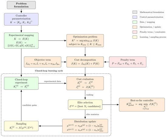
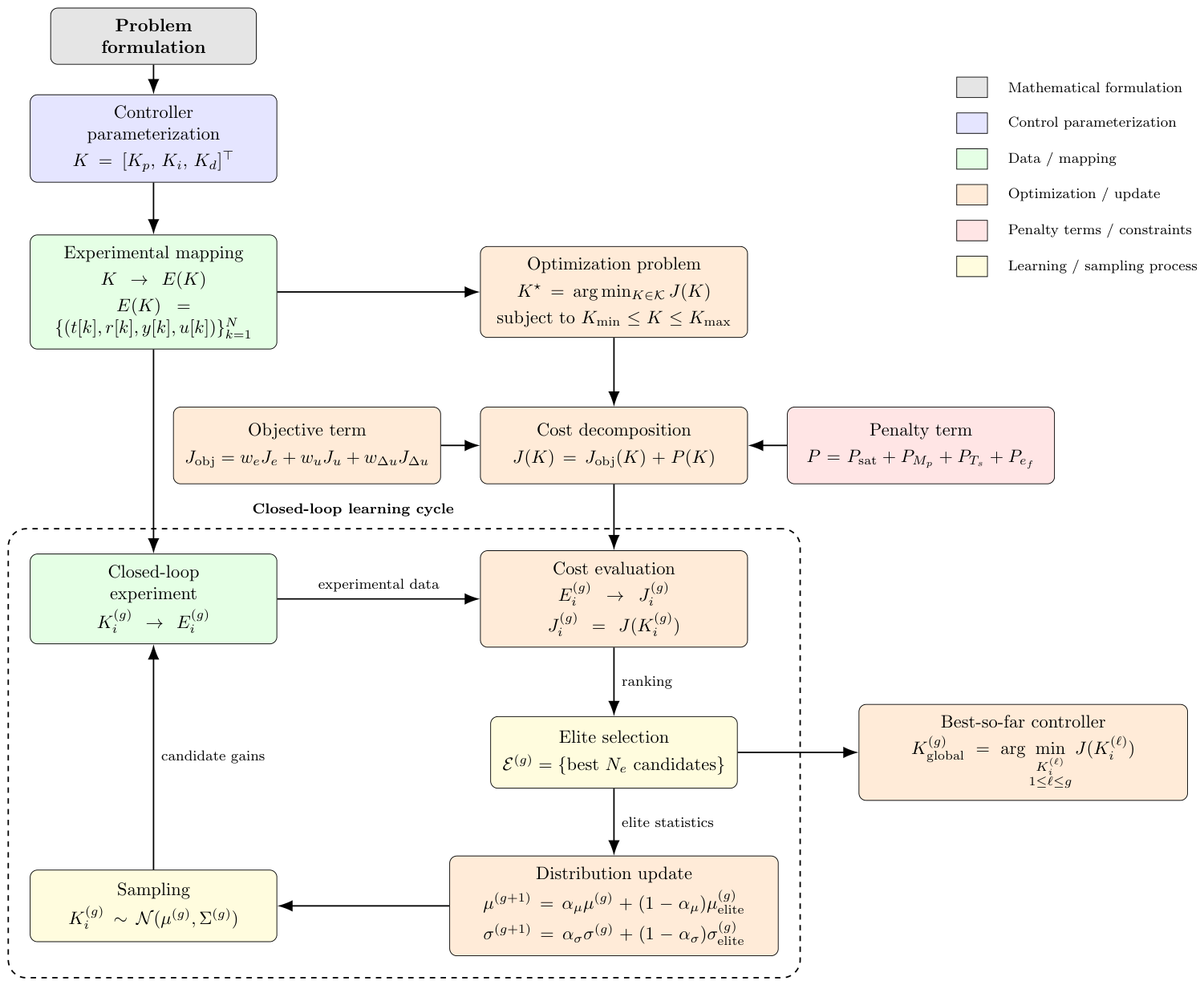
Figure 1 summarizes the complete mathematical workflow. A sampled gain vector is deployed on the physical system, converted into an experimental dataset, evaluated through the constrained performance index, and used to update the CEM sampling distribution.

Figure 1. Closed-loop experimental PID tuning pipeline based on the constrained Gaussian Cross-Entropy Method.

The iterative process is represented by

$$K_i^{\left(g\right)}⟶E_i^{\left(g\right)}⟶J_i^{\left(g\right)}⟶{\mathcal{E}}^{\left(g\right)}⟶\left({\mu }^{(g+1)},{\sigma }^{(g+1)}\right).$$

(39)

The embedded processor executes the deterministic PID loop during each experiment. Population generation, cost evaluation, candidate ranking, elite selection, and distribution updates are performed by the host computer between experiments.

3. Experimental Platform and Data Acquisition

This section describes the physical realization of the mathematical framework introduced in Section 2. The embedded system executes the deterministic PID feedback loop and records the experimental signals, whereas the host computer configures each run, stores the acquired dataset, evaluates the controller, and updates the CEM distribution between experiments.

3.1. Physical Experimental Platform

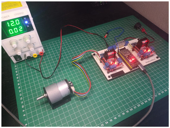
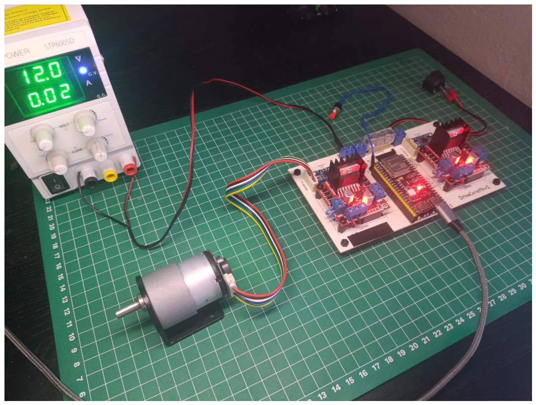
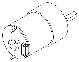
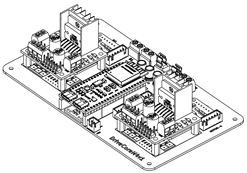
The experimental setup is shown in Figure 2. It consists of a JGB37-520 DC geared motor, a DriverCoreM4v1 embedded control module, a regulated DC power supply, and a host computer connected through a serial interface.

Figure 2. Physical platform used for experimental PID tuning, composed of a N-Hitech JGB37-520 DC geared motor (N-Hitech Co., Ltd., Gimpo, Republic of Korea), a DriverCoreM4v1 embedded control module (Oak Robotics, Guadalajara, Jalisco, Mexico), and a regulated DC power supply.

The JGB37-520 motor constitutes the physical plant. No parametric motor model is used during tuning. Shaft rotation is measured by an incremental encoder and converted into the angular position signal $y\left[k\right]$. The principal actuator specifications are summarized in Table 1.

Table 1. Main specifications of the JGB37-520 DC geared motor.

Graphic	Parameter	Specification
	Motor type	Brushed DC motor with gearbox
	Rated voltage	$12\mathrm{V}$
	No-load speed	$319\mathrm{rpm}$
	Load speed	$255\mathrm{rpm}$
	No-load current	$100\mathrm{mA}$
	Load current	$170\mathrm{mA}$
	Gear ratio	18.8:1
	Stall torque	$1.1\mathrm{kg}·\mathrm{cm}$
	Weight	Approximately $150\mathrm{g}$
JGB37-520	Measurement	Incremental encoder

The DriverCoreM4v1 module integrates the ESP32-S3 processor (Espressif Systems (Shanghai) Co., Ltd., Shanghai, China), the L298N-based actuation stage (STMicroelectronics, Geneva, Switzerland), and the encoder interface. Although the hardware supports additional channels and sensors, only the resources directly involved in the single-input single-output experiment are considered in this study. These resources are listed in Table 2.

Table 2. DriverCoreM4v1 resources used in the experimental implementation.

Graphic	Component	Specification
	Microcontroller	ESP32-S3, dual-core, up to $240\mathrm{MHz}$
	Motor driver	L298N H-bridge
	Actuation	PWM and digital direction signal
	Encoder interface	Quadrature A/B with interrupt processing
	Communication	UART/USB serial interface
	Input voltage	$8.4$–$12\mathrm{V}$
	Logic voltage	$3.3\mathrm{V}$
DriverCoreM4v1	Execution role	Feedback control and data acquisition

3.2. Embedded Feedback Architecture

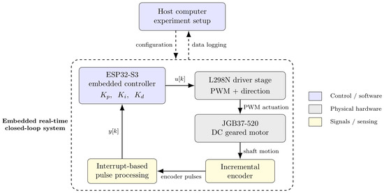
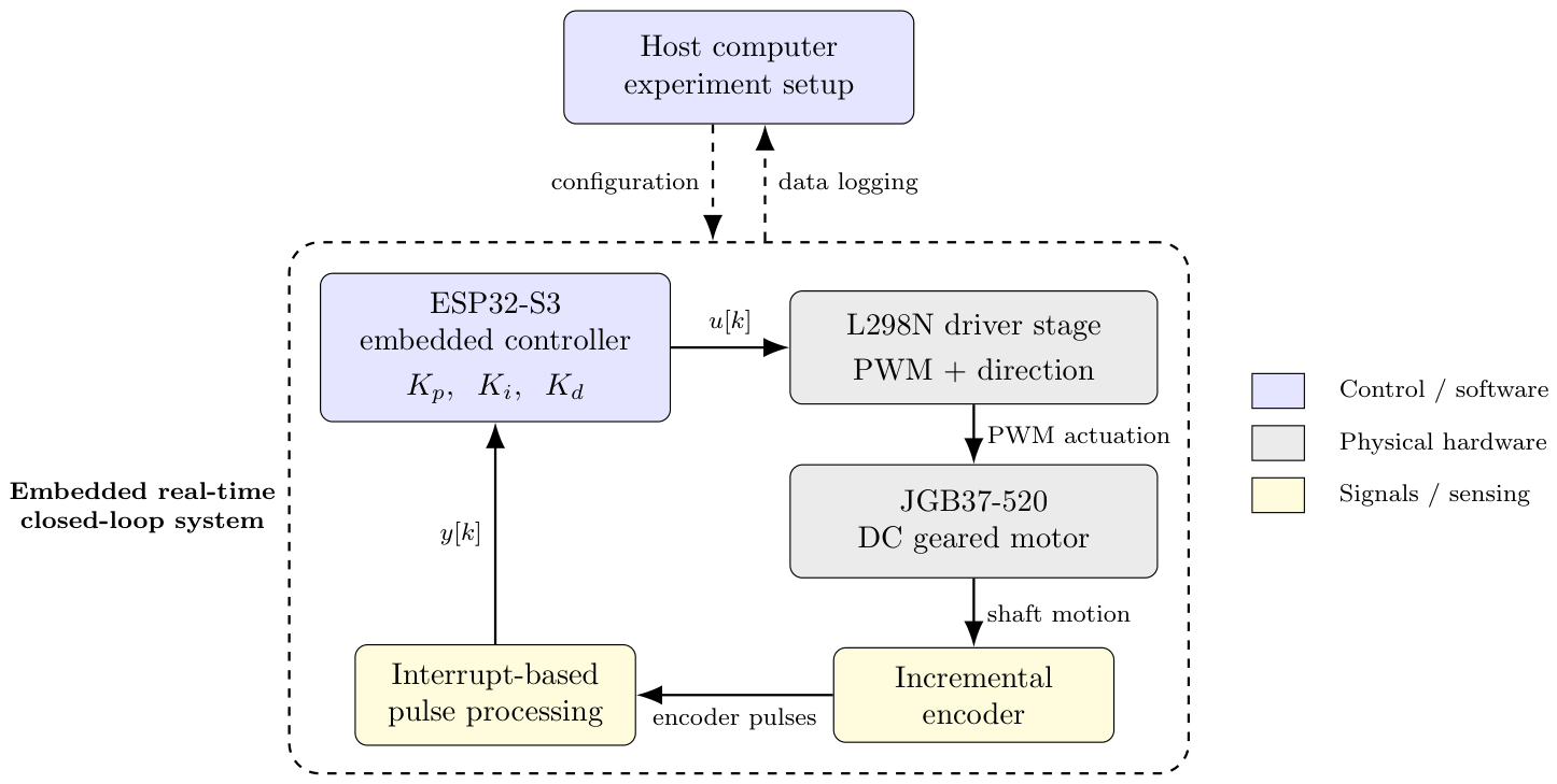
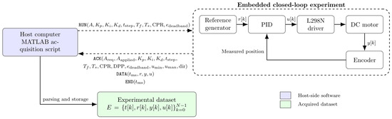
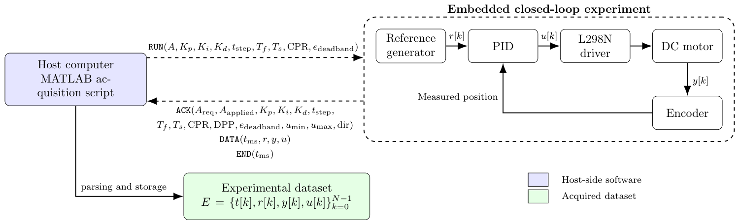
Figure 3 shows the host-embedded architecture and the physical feedback loop. At each sampling instant k, the ESP32-S3 acquires the angular position $y\left[k\right]$, calculates the error from the reference $r\left[k\right]$, evaluates the PID law, and applies the bounded PWM command $u\left[k\right]$ through the L298N driver. Motor motion is measured by the encoder and returned to the controller, closing the feedback loop.

Figure 3. Host-embedded control architecture. The feedback path formed by the PID controller, driver, motor, encoder, and measured output $y\left[k\right]$ is executed on the embedded platform. The host computer configures each experiment and processes the returned dataset between runs.

The PID gains defined in (1) are transmitted before each experiment and remain fixed throughout the run. The embedded processor performs only the time-critical operations: PID evaluation, encoder processing, actuator saturation, reference generation, sampling, and data transmission. Population generation, candidate ranking, elite selection, and CEM updates are performed on the host after the experiment has ended.

This separation ensures that the stochastic optimization process does not operate inside the sampling period $T_s$ and does not increase the memory or computational requirements of the embedded feedback loop.

3.3. Reference Signal and Operating Conditions

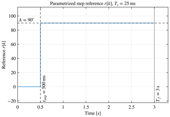
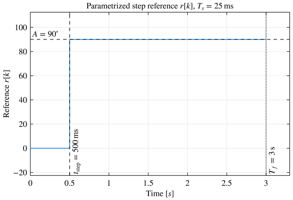
Each candidate controller is evaluated using a discrete-time step reference defined by the amplitude A, the step instant $t_{\mathrm{step}}$, the experiment duration $T_f$, and the sampling period $T_s$:

$$r\left[k\right]=\left\{\begin{array}{cc}0,\hfill & t\left[k\right]<t_{\mathrm{step}},\hfill \\ A,\hfill & t\left[k\right]\ge t_{\mathrm{step}}.\hfill \end{array}\right.$$

(40)

The nominal reference used during the learning campaign is shown in Figure 4.

Figure 4. Parametrized step reference used during the nominal PID tuning experiments.

The encoder count is converted into angular position using the specified counts per revolution. The controller output is represented by a signed PWM command. Table 3 summarizes the fixed operating conditions and hardware limits applied during the nominal learning campaign.

Table 3. Operating conditions and physical constraints of the experimental setup.

Quantity	Symbol	Value
PWM saturation	$u\left[k\right]$	$u\left[k\right]\in [-255,255]$
PWM resolution	–	8-bit
PWM frequency	–	$1000\mathrm{Hz}$
Sampling period	$T_s$	$25\mathrm{ms}$
Reference amplitude	A	${90}^{\circ }$ requested
Step time	$t_{\mathrm{step}}$	$500\mathrm{ms}$
Experiment duration	$T_f$	$3000\mathrm{ms}$
Encoder resolution	$\mathrm{CPR}$	$1336\mathrm{counts}/\mathrm{rev}$
Angular resolution	$\mathrm{DPP}$	$360/\mathrm{CPR}\mathrm{deg}/\mathrm{count}$
Error deadband	$e_{\mathrm{deadband}}$	$0.5^{\circ }$
Encoder direction	$\mathrm{dir}$	$-1$
Supply voltage	$V_{\mathrm{in}}$	$12\mathrm{V}$

These conditions remain unchanged while the gain vector K varies. Consequently, differences among the experimental responses are primarily associated with the evaluated PID parameters.

3.4. Serial Protocol and Dataset Construction

Each candidate controller is evaluated through a deterministic transaction between the host computer and the embedded system. The host transmits the requested gains and experimental configuration, the embedded controller confirms the applied values, and the closed-loop signals are returned as synchronized data packets.

Figure 5 shows the acquisition process. The figure distinguishes the physical feedback path executed by the embedded system from the bidirectional serial communication used for configuration and data transfer.

Figure 5. Experimental acquisition architecture. The embedded system executes the closed-loop feedback process and returns the measured dataset to the host through the ACK, DATA, and END messages.

The serial transaction is defined as

$$\mathtt{RUN}\left({\theta }_{\mathrm{req}}\right)⟶\mathtt{ACK}\left({\theta }_{\mathrm{app}}\right)⟶{\left\{\mathtt{DATA}\left(t_{\mathrm{ms}}\left[k\right],r\left[k\right],y\left[k\right],u\left[k\right]\right)\right\}}_{k=0}^{N-1}⟶\mathtt{END}\left(t_{\mathrm{ms}}[N-1]\right).$$

(41)

The requested configuration vector is

$${\theta }_{\mathrm{req}}=\left[\begin{array}{ccccccccc}A& K_p& K_i& K_d& t_{\mathrm{step}}& T_f& T_s& \mathrm{CPR}& e_{\mathrm{deadband}}\end{array}\right].$$

(42)

The configuration confirmed by the embedded system is

$${\theta }_{\mathrm{app}}=\left[\begin{array}{cc}{\theta }_{\exp }& {\theta }_{\mathrm{hw}}\end{array}\right],$$

(43)

where

$${\theta }_{\exp }=\left[\begin{array}{cccccccc}{A}_{\mathrm{req}}& A_{\mathrm{applied}}& K_p& K_i& K_d& t_{\mathrm{step}}& T_f& T_s\end{array}\right],$$

(44)

and

$${\theta }_{\mathrm{hw}}=\left[\begin{array}{cccccc}\mathrm{CPR}& \mathrm{DPP}& e_{\mathrm{deadband}}& u_{\min }& u_{\max }& \mathrm{dir}\end{array}\right],$$

(45)

the vector ${\theta }_{\exp }$ contains the applied reference, PID gains, and timing parameters, whereas ${\theta }_{\mathrm{hw}}$ contains the encoder conversion, deadband, actuator limits, and direction convention.

The ACK message allows the requested configuration to be compared with the values applied by the embedded system. This verification prevents a candidate from being evaluated under unconfirmed execution conditions.

Each DATA packet contains one sample of the dataset defined in (4). The time coordinate is reconstructed from the embedded millisecond counter as

$$t\left[k\right]={\displaystyle \frac{t_{\mathrm{ms}}\left[k\right]}{1000}}.$$

(46)

The expected number of samples is approximately

$$N\approx ⌊{\displaystyle \frac{T_f}{T_s}}⌋+1.$$

(47)

The actual value of N is obtained from the number of valid DATA packets received. The END message terminates the acquisition but does not add a sample to the dataset.

Table 4 summarizes the transmitted variables and their role in the communication protocol.

Table 4. Fields used in the experimental serial communication protocol.

Field	Description	Message Type
A	Requested reference amplitude	RUN
$K_p,K_i,K_d$	PID gains	RUN, ACK
$t_{\mathrm{step}}$	Step activation time	RUN, ACK
$T_f$	Experiment duration	RUN, ACK
$T_s$	Sampling period	RUN, ACK
$\mathrm{CPR}$	Encoder counts per revolution	RUN, ACK
$e_{\mathrm{deadband}}$	Error deadband	RUN, ACK
$A_{\mathrm{req}}$	Requested reference amplitude	ACK
$A_{\mathrm{applied}}$	Applied reference amplitude	ACK
$\mathrm{DPP}$	Degrees-per-pulse conversion	ACK
$u_{\min },u_{\max }$	PWM saturation limits	ACK
$\mathrm{dir}$	Encoder direction	ACK
$t_{\mathrm{ms}}$	Embedded timestamp	DATA, END
$r\left[k\right]$	Reference sample	DATA
$y\left[k\right]$	Angular-position sample	DATA
$u\left[k\right]$	Bounded controller command	DATA

The host stores the requested configuration, the applied configuration, the acquired signals, and the original protocol messages for every experiment. This structure provides traceability between each sampled controller, its physical execution conditions, and the performance cost subsequently assigned to it.

4. Host-Embedded Algorithmic Implementation

The mathematical framework introduced in Section 2 is implemented through two computational layers. The host computer manages the experimental campaign, evaluates the acquired datasets, and updates the CEM distribution. The embedded processor validates the requested configuration, executes the PID feedback law at the prescribed sampling period, and transmits the measured response.

The CEM operations are not executed inside the embedded control period. Consequently, population storage, candidate ranking, and distribution adaptation do not increase the computational burden of the real-time PID task.

4.1. Computational Partition and Execution Flow

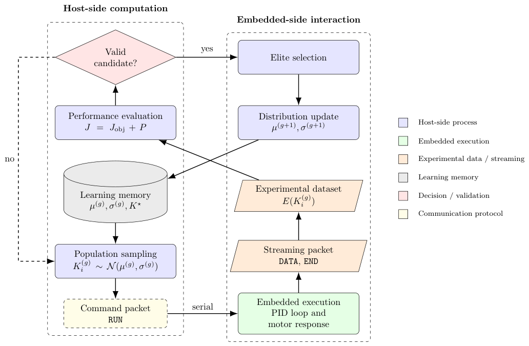
Figure 6 summarizes the allocation of operations between the host and embedded layers. For each sampled controller $K_i^{\left(g\right)}$, the host initiates an experiment through the protocol defined in (41). The embedded platform then executes the closed-loop experiment and returns the dataset $E_i^{\left(g\right)}$. The host evaluates $J_{\mathrm{obj}}$, P, and J, stores the resulting history, and updates the CEM state after the complete population has been evaluated.

Figure 6. Computational partition of the experimental PID tuning framework. Host-side optimization is performed between physical experiments, whereas feedback control and signal acquisition are executed on the embedded platform.

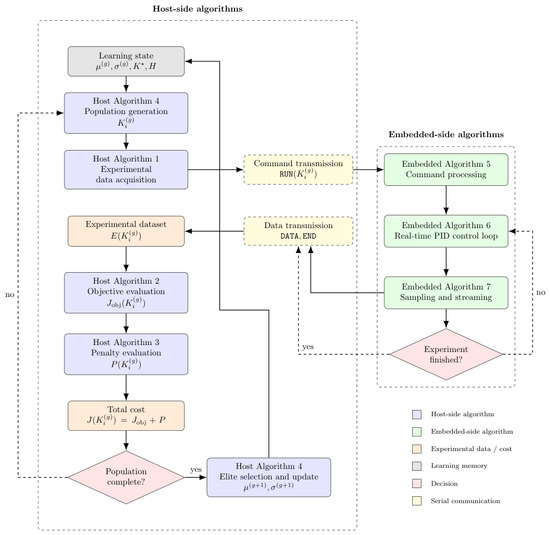
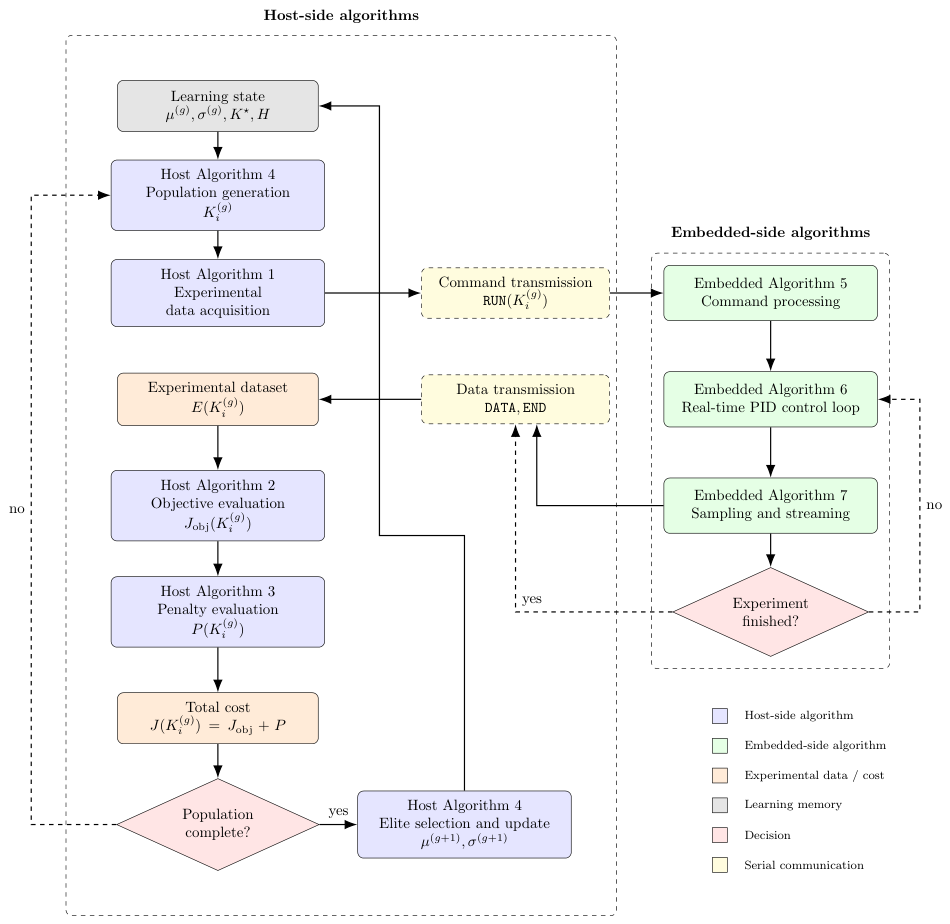
Figure 7 presents the sequence of host and embedded procedures. Algorithms 1–4 operate on the host computer. Algorithms 5–7 operate on the embedded controller.

Figure 7. Interaction among the host-side evaluation procedures, the CEM update, and the embedded closed-loop execution procedures.

4.2. Host-Side Procedures

The host-side implementation performs four functions: experimental acquisition, objective evaluation, penalty evaluation, and CEM adaptation. The acquisition procedure preserves both the requested and applied configurations so that every cost value remains traceable to its physical execution conditions.

Algorithm 1 Host-side experimental data acquisition

Require: Experiment configuration $cfg$, candidate gains K Ensure: Experimental dataset $E\left(K\right)$ 1: Validate the requested configuration 2: Construct the RUN packet using (41) 3: Open and initialize the serial interface 4: Transmit the RUN packet 5: Wait for the ACK response 6: if ACK is not received or an ERR message is returned then 7:     Report an acquisition failure 8:     return 9: end if 10: Parse and store the applied configuration ${\theta }_{\mathrm{app}}$ 11: Initialize the buffers for $t_{\mathrm{ms}}\left[k\right]$, $r\left[k\right]$, $y\left[k\right]$, and $u\left[k\right]$ 12: while END has not been received do 13:     Read the next serial message 14:     if the message is a valid DATA packet then 15:         Append the transmitted sample to the acquisition buffers 16:     else if the message is ERR or the acquisition timeout is exceeded then 17:         Report an acquisition failure 18:         return 19:     end if 20: end while 21: Convert $t_{\mathrm{ms}}\left[k\right]$ into $t\left[k\right]$ using (46) 22: Construct $E\left(K\right)$ according to (4) 23: Store the requested configuration, applied configuration, raw messages, and sampled signals 24: return $E\left(K\right)$

Algorithm 2 evaluates the nominal performance terms. The sampling period used in the numerical sums is estimated from the acquired time vector, thereby preserving consistency with the timestamps returned by the embedded system.

Algorithm 2 Host-side objective-function evaluation

Require: Experimental dataset $E\left(K\right)$, objective weights $w_e$, $w_u$, and $w_{\Delta u}$ Ensure: Objective value $J_{\mathrm{obj}}\left(K\right)$, performance metrics $met$ 1: Extract $t\left[k\right]$, $r\left[k\right]$, $y\left[k\right]$, and $u\left[k\right]$ 2: Truncate all signals to their common number of samples N 3: if $N<5$ then 4:     Report an invalid experiment 5:     return 6: end if 7: Estimate $T_s$ from the mean difference of consecutive timestamps 8: Compute $e\left[k\right]$ using (8) 9: Compute $\Delta u\left[k\right]$ 10: Evaluate $J_e$, $J_u$, and $J_{\Delta u}$ using (14)–(16) 11: Evaluate $J_{\mathrm{obj}}\left(K\right)$ using (17) 12: Compute $M_p$, $T_{\mathrm{set}}$, $e_f$, and ${\rho }_{\mathrm{sat}}$ 13: Store the objective components and response metrics in $met$ 14: return $J_{\mathrm{obj}}\left(K\right)$ and $met$

Algorithm 3 distinguishes acquisition failures, non-finite measurements, divergent responses, and finite responses that violate the prescribed performance thresholds.

Algorithm 3 Host-side penalty-function evaluation

Require: Experimental dataset $E\left(K\right)$, penalty parameters Ensure: Penalty value $P\left(K\right)$, penalty label $penLabel$, penalty components 1: Extract $t\left[k\right]$, $r\left[k\right]$, $y\left[k\right]$, and $u\left[k\right]$ 2: Truncate all signals to their common number of samples N 3: if $N<5$ then 4:     $P\left(K\right)\leftarrow J_{\mathrm{fail}}$ 5:     $penLabel\leftarrow \mathtt{short}\_\mathtt{experiment}$ 6:     return 7: end if 8: if any acquired value is non-finite then 9:      $P\left(K\right)\leftarrow J_{\mathrm{fail}}$ 10:     $penLabel\leftarrow \mathtt{nonfinite}\_\mathtt{data}$ 11:     return 12: end if 13: if ${\max }_k\left|y\left[k\right]\right|>y_{\mathrm{abs},\max }$ then 14:     Compute $P_y$ 15:     $P\left(K\right)\leftarrow J_{\mathrm{fail}}+P_y$ 16:     $penLabel\leftarrow \mathtt{divergence}$ 17:     return 18: end if 19: Compute ${\rho }_{\mathrm{sat}}$, $M_p$, $T_{\mathrm{set}}$, and $e_f$ 20: Compute $P_{\mathrm{sat}}$ using (21) 21: Compute $P_{M_p}$ using (23) 22: Compute $P_{T_{\mathrm{set}}}$ using (26) 23: Compute $P_{e_f}$ using (28) 24: Evaluate $P\left(K\right)$ using (29) 25: if $P\left(K\right)$ is non-finite then 26:     $P\left(K\right)\leftarrow J_{\mathrm{fail}}$ 27:     $penLabel\leftarrow \mathtt{invalid}\_\mathtt{penalty}$ 28:     return 29: end if 30: Assign $penLabel$ from the dominant active penalty 31: return $P\left(K\right)$, $penLabel$, and the penalty components

The complete host-side optimization is given in Algorithm 4. The procedure implements the constrained Gaussian CEM described in Section 2; it is not executed during an embedded sampling interval.

Algorithm 4 Host-side constrained Gaussian CEM for experimental PID tuning

Require: Gain bounds $K_{\min }$ and $K_{\max }$, initial $\mu$ and $\sigma$, population size $N_p$, elite count $N_e$, generation count $N_g$ Ensure: Best controller $K^{★}$, best cost $J^{★}$, experimental history $\mathcal{H}$ 1: Initialize a new campaign or load the stored learning state 2: Enforce the gain and dispersion bounds 3: for $g=1,\dots ,N_g$ do 4:     Sample $N_p$ bounded candidates using (30) 5:     Insert the best-so-far controller into the population when available 6:     for $i=1,\dots ,N_p$ do 7:         Assign $K_i^{\left(g\right)}$ to the experiment configuration 8:         Execute Algorithm 1 9:         if the acquisition is successful then 10:            Evaluate $J_{\mathrm{obj},i}^{\left(g\right)}$ using Algorithm 2 11:            Evaluate $P_i^{\left(g\right)}$ using Algorithm 3 12:            $J_i^{\left(g\right)}\leftarrow J_{\mathrm{obj},i}^{\left(g\right)}+P_i^{\left(g\right)}$ 13:         else 14:            $J_i^{\left(g\right)}\leftarrow J_{\mathrm{fail}}$ 15:            Mark the evaluation as unsuccessful 16:         end if 17:         Append the gains, costs, metrics, labels, and validity state to $\mathcal{H}$ 18:     end for 19:     Rank the population by increasing $J_i^{\left(g\right)}$ 20:     if the best candidate improves $J^{★}$ then 21:         Update $K^{★}$ and $J^{★}$ 22:     end if 23:     Select the successfully evaluated candidates among the first $N_e$ ranked positions 24:     if no elite candidate is available then 25:         Keep $\mu$ unchanged 26:         Expand and bound $\sigma$ 27:     else 28:         Compute ${\mu }_{\mathrm{elite}}^{\left(g\right)}$ using (34) 29:         Compute ${\sigma }_{\mathrm{elite}}^{\left(g\right)}$ using (35) 30:         Update $\mu$ using (36) 31:         Update $\sigma$ using (37) 32:     end if 33:     Store the updated learning state and experimental history 34: end for 35: return $K^{★}$, $J^{★}$, and $\mathcal{H}$

Algorithm 5 Embedded-side experiment configuration

Require: Serial input stream Ensure: Validated experiment state 1: if no serial command is available then 2:     return 3: end if 4: Read and parse the received command 5: if the command is not a valid RUN packet then 6:     Transmit ERR 7:     return 8: end if 9: Validate $T_f$, $t_{\mathrm{step}}$, $T_s$, $\mathrm{CPR}$, and $e_{\mathrm{deadband}}$ 10: if any requested parameter is inadmissible then 11:     Transmit ERR 12:     return 13: end if 14: Assign $K_p$, $K_i$, and $K_d$ 15: Configure $T_s$, $\mathrm{CPR}$, $\mathrm{DPP}$, and $e_{\mathrm{deadband}}$ 16: Quantize the requested reference amplitude 17: Reset the PID, reference, encoder, and sampling states 18: Activate the experiment 19: Transmit ACK with the applied configuration 20: Transmit the initial DATA sample at $t\left[0\right]=0$

4.3. Embedded-Side Procedures

The embedded implementation consists of command validation, PID evaluation, and periodic data transmission. These procedures use only the gains and experiment parameters transmitted before each run. No CEM population or learning memory is stored on the embedded processor.

Algorithm 6 reproduces the implemented PID computation and conditional-integration anti-windup mechanism. The bounded controller output $u\left[k\right]$ is recorded in the dataset. The command physically applied to the driver is denoted by $u_a\left[k\right]$ because the deadband policy may stop the actuator even when the computed bounded output is nonzero.

Algorithm 6 Embedded-side PID update

Require: Reference $r\left[k\right]$, measured position $y\left[k\right]$, PID gains, previous states Ensure: Bounded controller output $u\left[k\right]$, applied command $u_a\left[k\right]$ 1: Compute $e\left[k\right]\leftarrow r\left[k\right]-y\left[k\right]$ 2: Compute the proportional term $P\left[k\right]\leftarrow K_{p}e\left[k\right]$ 3: Compute the derivative term $D\left[k\right]\leftarrow K_d\left(e\left[k\right]-e[k-1]\right)/T_s$ 4: Compute the candidate integral term $\tilde{I}\left[k\right]\leftarrow I[k-1]+K_i{T}_{s}e\left[k\right]$ 5: Compute the trial output $\tilde{u}\left[k\right]\leftarrow P\left[k\right]+\tilde{I}\left[k\right]+D\left[k\right]$ 6: Compute the bounded trial output $u_{\mathrm{sat}}\left[k\right]$ 7: if $\tilde{u}\left[k\right]=u_{\mathrm{sat}}\left[k\right]$ then 8:     $I\left[k\right]\leftarrow \tilde{I}\left[k\right]$ 9: else if $\tilde{u}\left[k\right]>u_{\max }$ and $e\left[k\right]<0$ then 10:     $I\left[k\right]\leftarrow \tilde{I}\left[k\right]$ 11: else if $\tilde{u}\left[k\right]<u_{\min }$ and $e\left[k\right]>0$ then 12:     $I\left[k\right]\leftarrow \tilde{I}\left[k\right]$ 13: else 14:     $I\left[k\right]\leftarrow I[k-1]$ 15: end if 16: Compute $u\left[k\right]$ using (11) 17: Update the previous-error state 18: if $\left|e\left[k\right]\right|<e_{\mathrm{deadband}}$ then 19:     Reset the PID states 20:     $u_a\left[k\right]\leftarrow 0$ 21: else 22:     $u_a\left[k\right]\leftarrow u\left[k\right]$ 23: end if 24: return $u\left[k\right]$ and $u_a\left[k\right]$

Algorithm 7 Embedded-side sampling, actuation, and data streaming

Require: Active experiment, sampling period $T_s$, experiment duration $T_f$ Ensure: Serial DATA and END messages 1: if the experiment is inactive then 2:     return 3: end if 4: if the next sampling instant has not been reached then 5:     return 6: end if 7: Advance the sample counter 8: Compute the experiment time $t\left[k\right]$ 9: Update $r\left[k\right]$ using (40) 10: Read the encoder and compute $y\left[k\right]$ 11: Execute Algorithm 6 12: Apply $u_a\left[k\right]$ through the motor driver 13: Transmit $\mathtt{DATA}(t_{\mathrm{ms}}\left[k\right],r\left[k\right],y\left[k\right],u\left[k\right])$ 14: if $t\left[k\right]\ge T_f$ then 15:     Stop the actuator 16:     Reset the PID states 17:     Deactivate the experiment 18:     Transmit $\mathtt{END}\left(t_{\mathrm{ms}}\left[k\right]\right)$ 19: end if

The sampling scheduler invokes the PID update only when the prescribed sampling interval has elapsed. The scheduler also generates the reference, reads the encoder, applies the motor command, and transmits the corresponding data packet.

The resulting implementation preserves a deterministic embedded feedback task while allowing the host computer to perform episodic stochastic optimization from complete physical experiments.

5. Experimental Application

This section specifies the experimental conditions used to apply the formulation in Section 2 through the host-embedded implementation described in Section 4. Two stages were considered: a nominal learning campaign used to identify the PID gains and a subsequent validation stage performed with the selected controller fixed.

5.1. Nominal Learning Campaign

The nominal campaign was conducted using a step reference with amplitude $A={90}^{\circ }$. Each candidate controller was evaluated for $T_f=3\mathrm{s}$ using a sampling period of $T_s=25\mathrm{ms}$. The reference transition occurred at $t_{\mathrm{step}}=0.5\mathrm{s}$.

All physical and timing conditions remained fixed throughout the campaign. Only the gain vector K varied between candidate evaluations. The corresponding experimental conditions are summarized in Table 5.

Table 5. Experimental conditions used during the nominal learning campaign.

Parameter	Symbol	Value
Reference amplitude	A	${90}^{\circ }$
Step transition time	$t_{\mathrm{step}}$	$0.5\mathrm{s}$
Experiment duration	$T_f$	$3\mathrm{s}$
Sampling period	$T_s$	$25\mathrm{ms}$
Encoder resolution	$\mathrm{CPR}$	$1336\mathrm{counts}/\mathrm{rev}$
Angular resolution	$\mathrm{DPP}$	$360/1336\mathrm{deg}/\mathrm{count}$
Error deadband	$e_{\mathrm{deadband}}$	$0.5^{\circ }$
PWM limits	$u_{\min },u_{\max }$	$-255,255$
PWM frequency	–	$1000\mathrm{Hz}$
Supply voltage	$V_{\mathrm{in}}$	$12\mathrm{V}$

For each candidate $K_i^{\left(g\right)}$, the host transmitted the requested configuration, verified the applied parameters through the ACK message, acquired the dataset $E_i^{\left(g\right)}$, and evaluated the total cost according to (12). The motor and controller states were reset before every run so that all candidates were evaluated from equivalent initial conditions.

5.2. CEM Configuration

The PID search domain was defined as

$$K_{\min }={\left[\begin{array}{ccc}0& 0& 0\end{array}\right]}^{\top },K_{\max }={\left[\begin{array}{ccc}15& 10& 0.5\end{array}\right]}^{\top }.$$

(48)

The initial Gaussian distribution was parameterized by

$${\mu }^{\left(0\right)}={\left[\begin{array}{ccc}8& 6& 0.10\end{array}\right]}^{\top },{\sigma }^{\left(0\right)}={\left[\begin{array}{ccc}3& 2& 0.08\end{array}\right]}^{\top }.$$

(49)

The complete campaign comprised $N_g=60$ accumulated generations, with $N_p=8$ physical candidate evaluations per generation and $N_e=3$ elite positions. The learning state was stored after each generation, allowing execution to continue without resetting the sampling distribution or the best-so-far controller.

Table 6 summarizes the CEM parameters used in the application.

Table 6. CEM configuration used during experimental PID tuning.

Parameter	Symbol	Value
Accumulated generations	$N_g$	60
Population size	$N_p$	8
Elite positions	$N_e$	3
Mean smoothing factor	${\alpha }_{\mu }$	$0.7$
Dispersion smoothing	${\alpha }_{\sigma }$	$0.8$
Initial mean	${\mu }^{\left(0\right)}$	${[8,6,0.10]}^{\top }$
Initial dispersion	${\sigma }^{\left(0\right)}$	${[3,2,0.08]}^{\top }$
Minimum dispersion	${\sigma }_{\min }$	${[0.15,0.15,0.01]}^{\top }$
Maximum dispersion	${\sigma }_{\max }$	${[3.75,2.50,0.125]}^{\top }$
Best-so-far injection	–	Enabled
Failure cost	$J_{\mathrm{fail}}$	${10}^{12}$

The sampling bounds, dispersion limits, smoothing factors, and best-so-far injection remained unchanged throughout the campaign. If no successfully evaluated candidate was available among the first $N_e$ ranked positions, the dispersion was expanded according to the rule defined in Section 2.

5.3. Objective and Penalty Configuration

The objective weights were selected to prioritize angular tracking while retaining regularization terms for control effort and command variation:

$$w_e=1,w_u={10}^{-4},w_{\Delta u}={10}^{-3}.$$

(50)

The penalty thresholds and coefficients are listed in Table 7. These values define the admissibility requirements applied uniformly to all candidate experiments.

Table 7. Penalty thresholds and coefficients used during the nominal campaign.

Penalty	Threshold	Coefficient	Value
Saturation	${\rho }_{\max }=0.10$	${\lambda }_{\mathrm{sat}}$	$5\times {10}^4$
Overshoot	$M_{p,\max }=15\%$	${\lambda }_{M_p}$	$2\times {10}^3$
Settling time	$T_{\mathrm{set},\max }=2\mathrm{s}$	${\lambda }_{T_{\mathrm{set}}}$	$5\times {10}^2$
Final error	$e_{f,\max }=2^{\circ }$	${\lambda }_{e_f}$	$2\times {10}^3$
Divergence	$y_{\mathrm{abs},\max }=1.5A$	${\lambda }_y$	$5\times {10}^4$

The settling band was defined using $\beta =0.02$, corresponding to a relative band of $2\%$ around the final reference. The final tracking error was estimated from the last $n_f=10$ acquired samples. These quantities were fixed before the learning campaign and were not modified in response to the observed results.

5.4. Evaluation Protocol Under Reference-Amplitude Variations

After completing the nominal learning campaign, the best-so-far controller defined by (38) was fixed. No further sampling, adaptation, or parameter update was performed during the subsequent evaluation experiments.

The subsequent experiments evaluated the fixed controller using positive and negative step amplitudes different from the nominal learning condition. The sampling period, step instant, experiment duration, encoder conversion, actuator limits, deadband, and supply voltage remained unchanged. Consequently, the requested reference amplitude was the only deliberately modified experimental variable.

For an amplitude $A\in {\mathcal{A}}_{\mathrm{eval}}$, the acquired evaluation dataset was denoted by

$$E_A={\left\{t\left[k\right],r_A\left[k\right],y_A\left[k\right],u_A\left[k\right]\right\}}_{k=0}^{N-1}.$$

(51)

The initial and final reference levels were estimated directly from each acquired reference sequence and denoted by $r_0$ and $r_f$, respectively. For $r_f\ne r_0$, the normalized reference and output were defined as

$$r_N\left[k\right]={\displaystyle \frac{r_A\left[k\right]-r_0}{r_f-r_0}},$$

(52)

and

$$y_N\left[k\right]={\displaystyle \frac{y_A\left[k\right]-r_0}{r_f-r_0}}.$$

(53)

The normalized tracking error was

$$e_N\left[k\right]=r_N\left[k\right]-y_N\left[k\right].$$

(54)

Because all validation experiments used the same sampling period, transition instant, and final time, the normalized responses were compared at corresponding sampling instants. For the evaluated set containing $N_A$ amplitudes, the mean normalized response was computed as

$${\overline{y}}_N\left[k\right]={\displaystyle \frac{1}{N_A}}{\displaystyle \sum _{j=1}^{N_A}}{y}_{N,j}\left[k\right],$$

(55)

and its sample standard deviation was

$${\sigma }_{y_N}\left[k\right]=\sqrt{{\displaystyle \frac{1}{N_A-1}}\sum _{j=1}^{N_A}{\left(y_{N,j}\left[k\right]-{\overline{y}}_N\left[k\right]\right)}^2}.$$

(56)

The evaluation considered the raw and normalized responses, normalized tracking error, overshoot, settling time, final error, total cost, and applied control signals. These quantities were computed using the fixed controller and were not used to perform any additional retuning. The resulting observations are restricted to the tested reference amplitudes and do not constitute a general robustness or stability assessment.

6. Results and Discussion

This section analyzes the experimental behavior of the constrained Gaussian CEM and the closed-loop response obtained with the selected PID controller. The results correspond to one complete learning campaign comprising $N_g=60$ accumulated generations and $N_p=8$ physical evaluations per generation. Therefore, the reported convergence curves characterize the internal evolution of one stochastic realization and should not be interpreted as run-to-run statistical evidence.

6.1. Generation-Level Cost Evolution

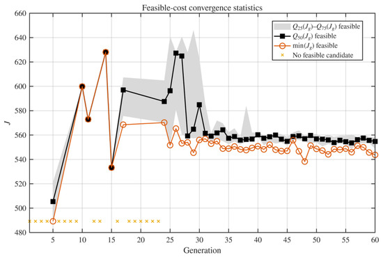
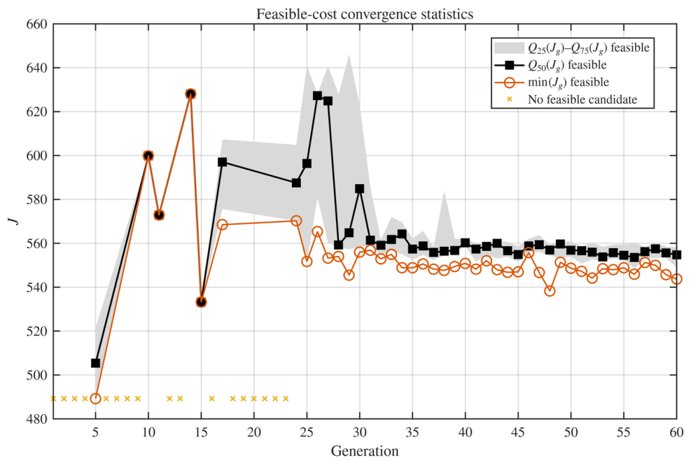
Figure 8 presents the distribution of feasible costs at each generation. The interquartile interval and median describe the transition from broad exploratory evaluations toward a more concentrated range of feasible costs within the reported campaign. Generations without feasible candidates correspond to sampled controllers that violated at least one experimental requirement or failed to produce an admissible response.

Figure 8. Generation-level feasible-cost statistics. The interquartile interval and median describe the concentration of admissible candidate costs during the CEM campaign.

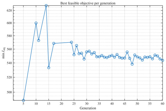
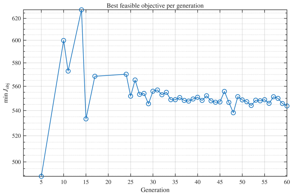
The minimum feasible objective value obtained at each generation is shown in Figure 9. The largest cost reduction occurs during the initial exploratory stage. After approximately generation $g=30$, the best feasible values fluctuate within a comparatively narrow interval, indicating that subsequent populations repeatedly sampled controllers with similar objective values within this stochastic realization.

Figure 9. Best feasible objective value obtained at each generation of the experimental campaign.

These results show within-campaign concentration of the feasible objective values. However, they do not constitute a formal convergence proof or characterize the variability of the final solution across independent campaigns and initializations.

6.2. Evolution of the CEM Sampling Distribution

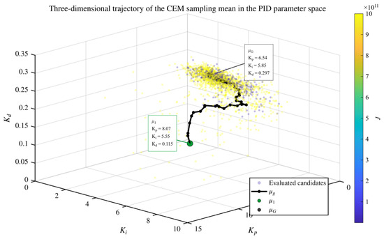
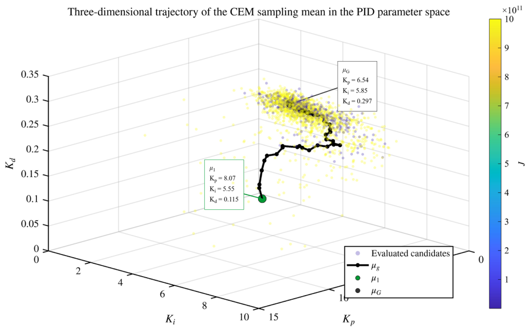
Figure 10 shows the trajectory of the Gaussian sampling mean in the three-dimensional PID parameter space. Within the reported campaign, the distribution center moves from the initial condition toward a localized region associated with lower experimentally measured costs.

Figure 10. Three-dimensional trajectory of the CEM sampling mean in the PID parameter space.

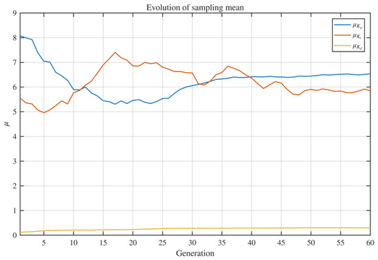
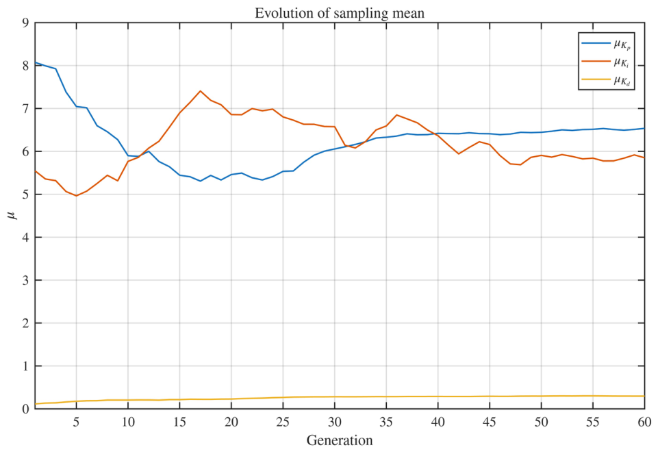
The componentwise evolution of the sampling mean is presented in Figure 11. The proportional and integral components exhibit the largest displacement during the initial generations, whereas the derivative component remains within the narrower interval imposed by its admissible range. The revised figure uses differentiated colors and line styles to improve visual separation among the three gain components.

Figure 11. Evolution of the CEM sampling mean components. Distinct color and line encodings are used for ${\mu }_{K_p}$, ${\mu }_{K_i}$, and ${\mu }_{K_d}$.

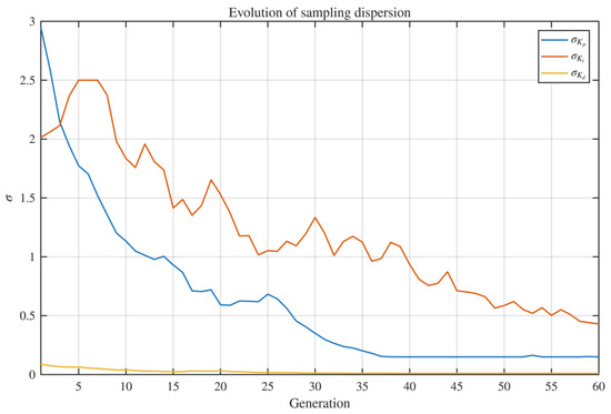
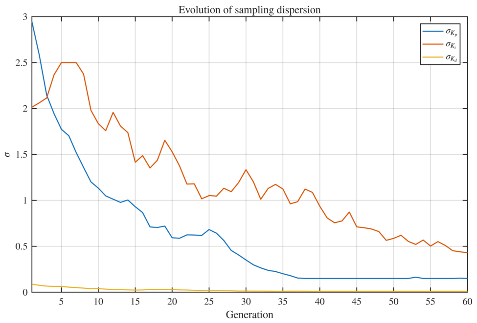
Figure 12 shows the corresponding exploration scales. Their reduction describes the progressive concentration of the sampling distribution observed during the reported realization. The nonzero lower bounds imposed on $\sigma$ prevent complete distribution collapse and preserve local exploration.

Figure 12. Evolution of the componentwise CEM sampling dispersion.

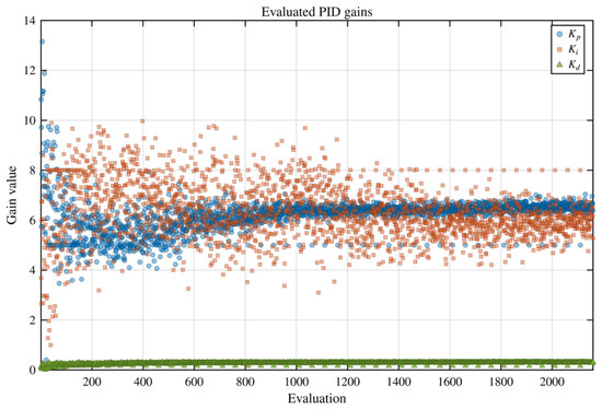
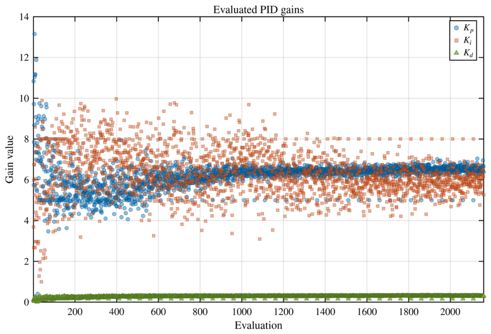
The complete set of evaluated gains is shown in Figure 13. The early population samples cover a broad portion of the admissible domain, whereas later candidates concentrate near the final sampling region. This behavior results directly from elite selection and the smoothed updates defined in (36) and (37).

Figure 13. PID gains physically evaluated during the complete CEM campaign.

The observed adaptation is consistent with the standard behavior of CEM and is not presented as a new stochastic optimization mechanism. The contribution lies in connecting this update process to the physical mapping $K⟶E\left(K\right)⟶J\left(K\right)$ through a traceable host-embedded implementation.

6.3. Selected Controller and Reference-Amplitude Evaluation

The controller with the lowest recorded cost during the nominal campaign was

$$K^{★}={\left[\begin{array}{ccc}4.999010& 8.003378& 0.156947\end{array}\right]}^{\top },$$

(57)

with recorded cost

$$J^{★}=489.265473.$$

(58)

The gains were fixed during the validation stage. No CEM update, adaptation, or retuning was performed after selecting $K^{★}$. Therefore, the following results describe the response of one fixed controller under reference amplitudes different from the nominal learning condition.

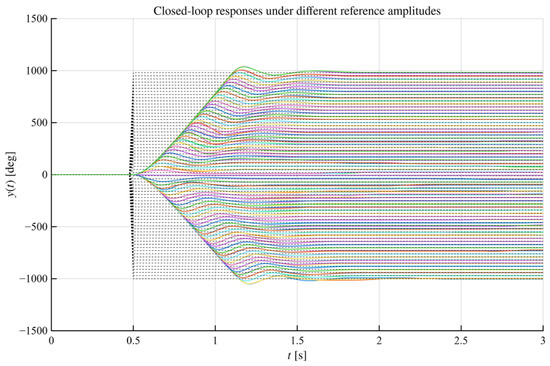
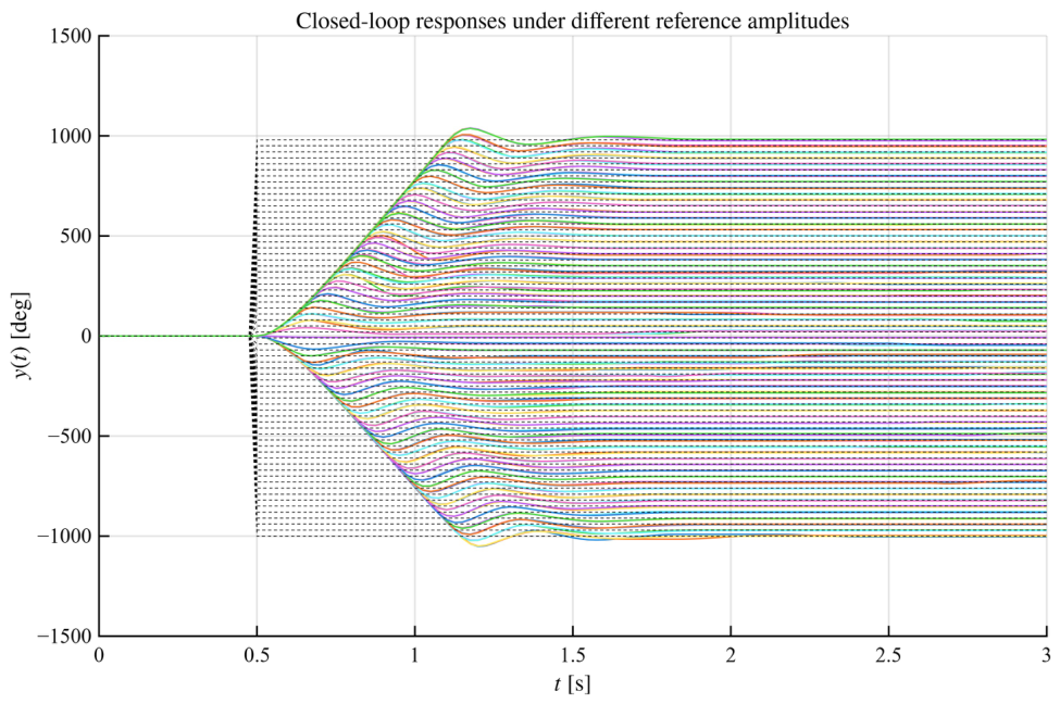
Figure 14 presents the measured angular responses. No divergent trajectory was observed for the evaluated positive and negative references, although their absolute transient characteristics vary with the requested amplitude. This observation is restricted to the tested reference amplitudes and operating conditions.

Figure 14. Closed-loop responses obtained with the fixed controller $K^{★}$ under different reference amplitudes.

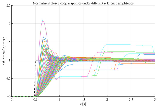
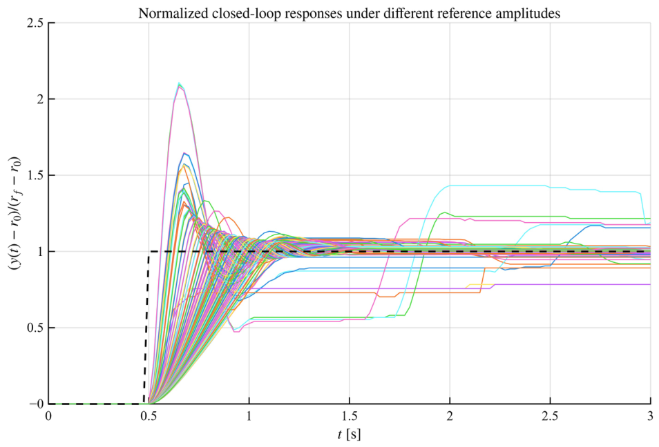
The normalized responses defined in Section 5 are shown in Figure 15. Normalization removes the amplitude and sign of the reference transition and allows the transient shapes to be compared on a common scale.

Figure 15. Normalizedclosed-loop responses obtained with the fixed controller under reference amplitude variations.

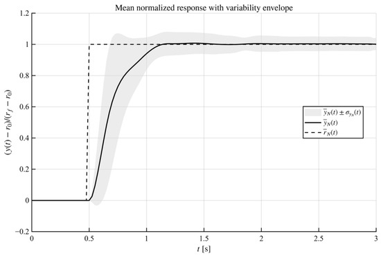
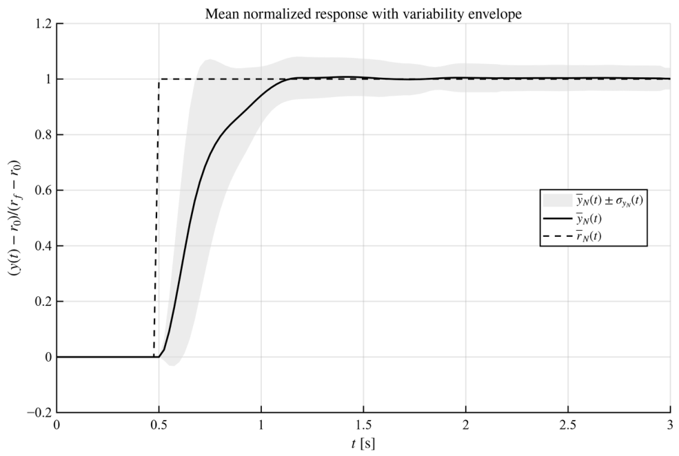
Figure 16 presents the mean normalized trajectory and its variability envelope. The concentration of the responses indicates that the measured trajectories exhibit similar normalized transient profiles over the evaluated amplitude set. The corresponding envelope describes variability across different reference conditions and should not be interpreted as a statistical confidence interval obtained from repeated independent trials.

Figure 16. Mean normalized response and sample standard-deviation envelope over the amplitude validation set.

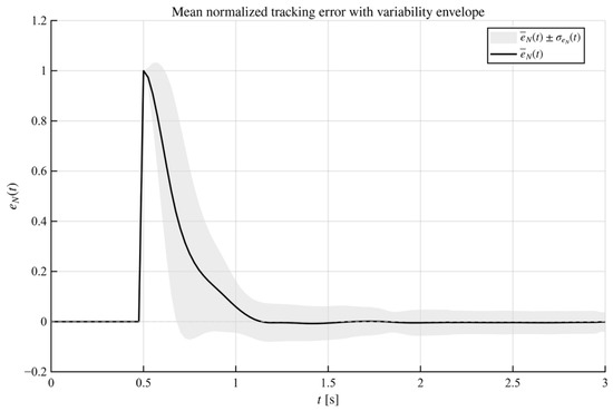
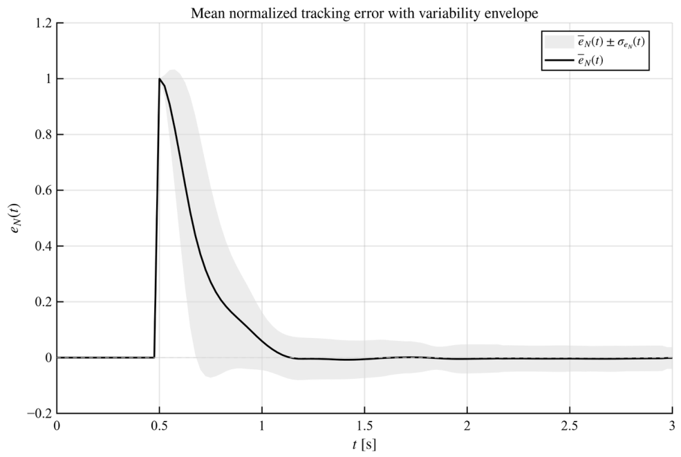
The normalized tracking-error statistics are shown in Figure 17. The mean normalized error decreases after the transient interval, while the envelope describes the dispersion associated with the different reference amplitudes. Because each amplitude represents a different experimental condition, this dispersion does not quantify run-to-run stochastic variability.

Figure 17. Mean normalized tracking error and variability envelope for the amplitude-validation experiments.

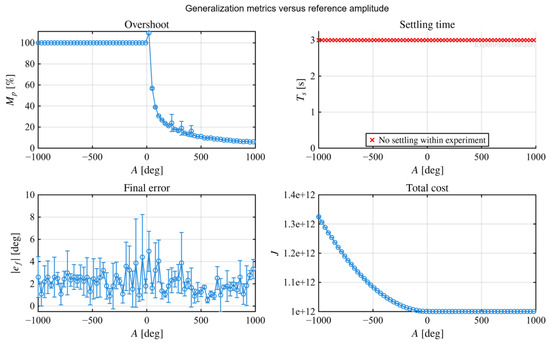
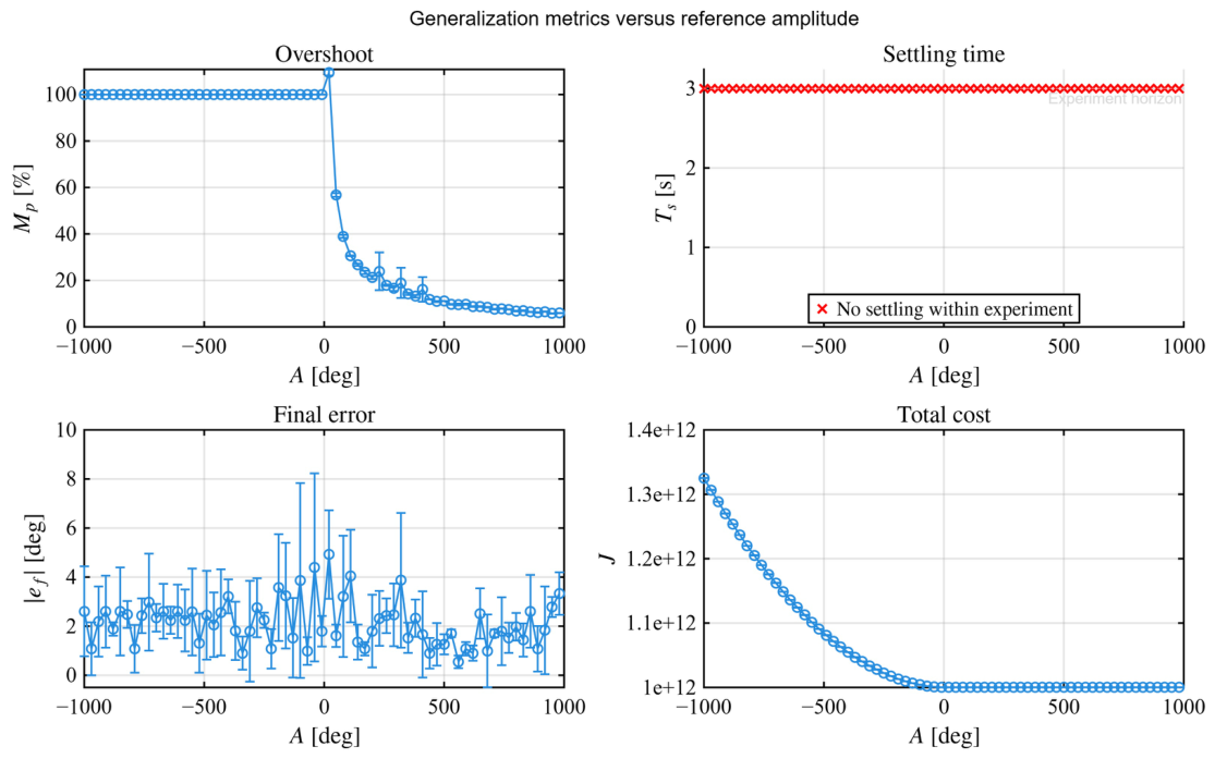
Figure 18 summarizes the overshoot, settling time, final error, and total cost obtained for each validation amplitude. These quantities characterize the measured behavior of the fixed controller when the reference differs from the nominal tuning condition.

Figure 18. Closed-loop performance metrics obtained with the fixed controller under reference amplitude variations.

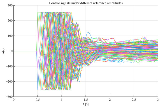
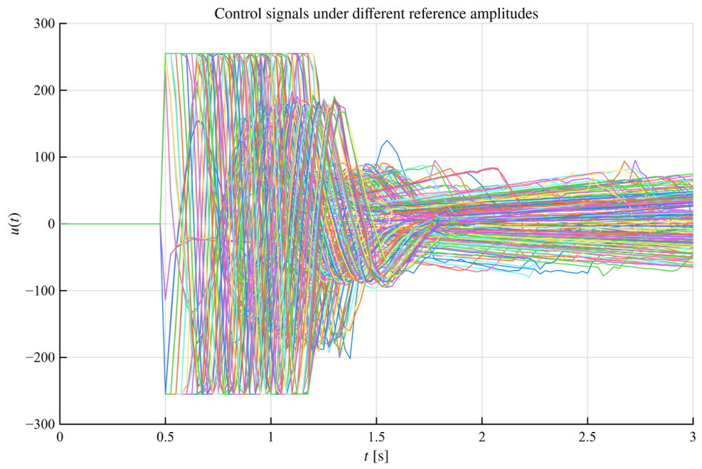
The corresponding bounded controller commands are shown in Figure 19. The trajectories exhibit the largest corrective action immediately after the reference transition and remain within the actuator limits imposed by the embedded implementation.

Figure 19. Bounded controller commands generated by the fixed controller during the amplitude validation experiments.

The experiments show that the selected controller produced finite tracking responses and control commands within the imposed actuator limits for the evaluated amplitude set. These observations do not constitute an analytical stability certificate or a robustness guarantee against untested loads, supply variations, parameter changes, measurement conditions, or external disturbances.

6.4. Computational Burden and Experimental Timing

The host-embedded architecture separates the real-time feedback task from the episodic optimization procedure. During each sampling interval, the embedded processor evaluates the PID law, processes the encoder measurement, applies actuator saturation, and transmits one data sample. The number of arithmetic operations does not depend on the population size or generation count. Its computational complexity per sample is therefore constant:

$$\mathcal{O}\left(1\right).$$

(59)

These complexity expressions describe the scaling of the implemented computational partition. They do not constitute a formal worst-case execution-time analysis of the embedded software. The CEM population, experimental history, ranking operation, and sampling-distribution parameters are stored and processed on the host computer. For a gain dimension $d=3$, the population-storage requirement is

$$\mathcal{O}\left(N_{p}d\right),$$

(60)

and ranking the population requires

$$\mathcal{O}\left(N_p\log N_p\right).$$

(61)

These operations are performed between experiments and do not compete with the embedded sampling deadline $T_s=25\mathrm{ms}$.

The total number of physical evaluations in the reported campaign was

$$N_{\exp }=N_g{N}_p=60\times 8=480.$$

(62)

Because each experiment lasted $T_f=3\mathrm{s}$, the minimum physical execution time was

$$T_{\mathrm{campaign},\min }=N_{\exp }{T}_f=480\times 3\mathrm{s}=1440\mathrm{s}=24\min .$$

(63)

This value excludes serial initialization, acknowledgment delays, file storage, motor resetting, and host-side processing. The actual campaign duration is consequently greater than $24\min$.

The real-time claim is therefore restricted to the embedded PID execution level. The complete tuning process is not an online gain-adaptation law operating within each sampling interval. It is an experimental commissioning or episodic-retuning procedure. The reduction in modeling effort is obtained at the cost of repeated physical experiments, actuator usage, and campaign duration.

6.5. Positioning Relative to Existing Data-Driven PID Tuning

The use of experimental data for PID tuning is well established. Online minimum variance tuning [11], one-shot fictitious-reference design [12], and constrained data-driven optimization with stability considerations [13] provide alternatives with different requirements concerning data volume, auxiliary assumptions, and formal guarantees.

Population-based experimental tuning has also been investigated through evolutionary comparisons [23] and safe experimentation dynamics [24]. One-shot approaches generally require fewer physical evaluations than the iterative implementation considered here. Methods that explicitly derive stability conditions provide analytical guarantees that are not supplied by the present penalty-based experimental formulation.

The distinguishing element of the present study is the end-to-end experimental architecture. Each sampled gain vector is physically deployed, the requested and applied configurations are recorded, the complete dataset is stored, physical penalties are evaluated, and the CEM state is updated outside the embedded feedback loop. The contribution is therefore methodological and architectural rather than a new PID-tuning principle or a new version of CEM.

Table 8 provides a qualitative contextualization based on the reported scope of the cited approaches. It does not constitute a quantitative benchmark because the alternative methods were not implemented on the same physical platform. A controlled comparison of convergence speed, final performance, and experimental cost would require common hardware, reference signals, constraints, initialization rules, stopping criteria, and performance indices.

Table 8. Scope of representative recent data-driven PID tuning approaches and the present framework.

Approach	Primary Objective	Data or Experimental Requirement	Relation to the Present Study
Zhu et al. [11]	Online minimum-variance PID auto-tuning	Operational closed-loop data	Emphasizes online tuning rather than a host-embedded episodic campaign
Yonezawa et al. [12]	One-shot data-driven fractional-order PID design	Single experimental dataset	Requires fewer physical evaluations than the iterative CEM procedure
Massoud and Libby [23]	Comparison of evolutionary PID optimizers	Simulation and physical experiments	Provides an algorithmic benchmark, whereas the present study emphasizes experimental traceability
Saat et al. [24]	Safe experimentation-based intelligent PID control	Repeated stochastic evaluations	Includes repeated-run statistical analysis not yet performed in the present campaign
Liu et al. [13]	Constrained data-driven optimal PID tuning	Measured data and formal closed-loop conditions	Provides stronger analytical guarantees than the experimental formulation considered here
Present framework	Traceable host-embedded experimental PID tuning	Repeated physical closed-loop experiments	Integrates deployment, acquisition, constrained evaluation, and episodic CEM updates

6.6. Limitations and Scope of the Evidence

The results are subject to four principal limitations. First, only one complete CEM campaign was analyzed. The 480 candidate evaluations characterize the internal evolution of that campaign but are not independent repetitions of the complete stochastic optimization procedure. Consequently, the present results do not estimate the run-to-run mean or variance of $J^{★}$, $K^{★}$, $M_p$, and $T_{\mathrm{set}}$, nor do they establish insensitivity to stochastic initialization.

Second, the objective and penalty coefficients were fixed before the campaign. Their values establish the relative importance of tracking, actuation, smoothness, and constraint violations, but the present results do not quantify how perturbations of these coefficients affect the selected gains. Accordingly, no claim of insensitivity to the objective or penalty configuration is made.

Third, no alternative model-free tuning method was executed on the same motor platform. The current results document the execution and internal consistency of the proposed architecture but do not demonstrate superiority in convergence speed, control performance, or experimental efficiency.

Fourth, the penalty terms encode experimentally selected admissibility thresholds and operational safeguards. They do not provide necessary or sufficient analytical stability conditions for the closed-loop PID system. A formal stability analysis would require an explicit or bounded representation of the plant dynamics together with assumptions that are outside the scope of the present model-free experimental formulation.

Finally, the validation considers reference-amplitude changes while maintaining the same actuator, supply voltage, mechanical load, sampling period, and hardware configuration. Performance under disturbances, load changes, measurement noise, supply variations, and long-term actuator variation remains outside the experimental scope of this study.

7. Conclusions

This study formulated and experimentally implemented a closed-loop PID tuning architecture for a DC motor actuator without requiring an explicit parametric plant model. The complete process was defined through the mapping $K⟶E\left(K\right)⟶J\left(K\right)$, which connects each PID gain vector with its physical closed-loop experiment, acquired dataset, and constrained performance evaluation.

A constrained Gaussian Cross-Entropy Method was adopted as the search mechanism. The contribution does not lie in the development of a new stochastic optimizer, but in the integration of physical controller deployment, structured serial acquisition, requested-versus-applied parameter verification, objective and penalty evaluation, persistent learning memory, and host-side distribution adaptation within a reproducible host-embedded architecture.

The implementation separates the two relevant computational time scales. The embedded processor executes the deterministic PID controller, encoder processing, actuator saturation, reference generation, and data transmission at the prescribed sampling period. Population sampling, cost evaluation, candidate ranking, elite selection, and CEM updates are performed by the host computer between experiments. Consequently, the proposed method supports real-time embedded PID execution, whereas the complete tuning procedure constitutes an episodic commissioning or retuning process rather than an online gain-adaptation law.

Within the reported experimental campaign, the CEM distribution progressively concentrated within a localized region of the admissible PID space. The selected controller produced finite tracking responses and control commands within the imposed limits for the evaluated reference-amplitude variations. These results document the internal consistency and experimentally observed feasibility of the proposed pipeline under the considered sampling, saturation, encoder, communication, and actuator conditions.

The conclusions are limited to the reported platform and experimental conditions. The present study analyzes one complete stochastic campaign, does not include repeated independent optimizations, and does not provide a quantitative comparison with alternative model-free tuning methods on the same testbed. Moreover, the sensitivity of the selected controller to objective and penalty coefficients has not yet been quantified. Therefore, the current results demonstrate experimentally observed feasibility and traceability under the reported conditions, but they do not establish run-to-run statistical consistency, global optimality, analytical closed-loop stability, or superiority over existing tuning approaches.

The penalty-based admissibility mechanism used during the physical search does not provide an analytical closed-loop stability certificate. Establishing such a certificate would require an explicit or bounded plant representation and additional assumptions that are outside the scope of the present model-free experimental study.

Future work may consider repeated independent campaigns to characterize the dispersion of the learned gains and closed-loop metrics, sensitivity analysis of the objective and penalty coefficients, controlled comparisons with representative model-free and evolutionary PID tuning methods, and stability-oriented extensions based on an explicit or bounded plant representation. Further extensions will address load disturbances, supply variations, multi-actuator systems, higher-dimensional controller structures, and experimental platforms with nonlinear, underactuated, or open-loop unstable dynamics.

References

- Ang, K.H.; Chong, G.; Li, Y. PID control system analysis, design, and technology. IEEE Trans. Control Syst. Technol. 2005, 13, 559–576. [Google Scholar] [CrossRef] [Scilit]
- Vilanova, R.; Visioli, A. PID Control in the Third Millennium: Lessons Learned and New Approaches; Springer: Berlin/Heidelberg, Germany, 2012. [Google Scholar]
- Skogestad, S. Simple Analytic Rules for Model Reduction and PID Controller Tuning. J. Process Control 2003, 13, 291–309. [Google Scholar] [CrossRef] [Scilit]
- Wang, Q.G.; Lee, T.H.; Fung, H.W.; Bi, Q.; Zhang, Y. PID Tuning for Improved Performance. IEEE Trans. Control Syst. Technol. 2001, 9, 674–685. [Google Scholar] [CrossRef]
- Ljung, L. System Identification: Theory for the User, 2nd ed.; Prentice Hall: Upper Saddle River, NJ, USA, 1999. [Google Scholar]
- Bohlin, T. Practical Grey-Box Process Identification: Theory and Applications; Springer: London, UK, 2006. [Google Scholar] [CrossRef] [Scilit]
- Hjalmarsson, H.; Gevers, M.; Gunnarsson, S.; Lequin, O.A. Iterative Feedback Tuning: Theory and Applications. IEEE Control Syst. Mag. 1998, 18, 26–41. [Google Scholar] [CrossRef] [Scilit]
- Formentin, S.; Savaresi, S.M.; Re, L.D. Non-Iterative Direct Data-Driven Controller Tuning for Multivariable Systems: Theory and Application. IET Control Theory Appl. 2012, 6, 1250–1257. [Google Scholar] [CrossRef] [Scilit]
- Karimi, A.; Bonvin, D. A Data-Driven Approach to Robust Control of Multivariable Systems by Convex Optimization. Automatica 2007, 43, 572–581. [Google Scholar] [CrossRef] [Scilit]
- Hou, Z.S.; Jin, S.T. A Novel Data-Driven Control Approach for a Class of Discrete-Time Nonlinear Systems. IEEE Trans. Control Syst. Technol. 2011, 19, 1549–1558. [Google Scholar] [CrossRef] [Scilit]
- Zhu, N.; Gao, X.T.; Huang, C.Q. A Data-Driven Approach for On-Line Auto-Tuning of Minimum Variance PID Controller. ISA Trans. 2022, 130, 325–342. [Google Scholar] [CrossRef] [Scilit] [PubMed]
- Yonezawa, A.; Yonezawa, H.; Yahagi, S.; Kajiwara, I. Practical One-Shot Data-Driven Design of Fractional-Order PID Controller: Fictitious Reference Signal Approach. ISA Trans. 2024, 152, 208–216. [Google Scholar] [CrossRef] [Scilit] [PubMed]
- Liu, N.; Chai, T.; Zhang, Y.; Gao, W. Data-Driven Optimal Tuning of PID Controller Parameters. Sci. China Inf. Sci. 2025, 68, 172201. [Google Scholar] [CrossRef] [Scilit]
- Bristow, D.A.; Tharayil, M.; Alleyne, A.G. A Survey of Iterative Learning Control. IEEE Control Syst. Mag. 2006, 26, 96–114. [Google Scholar] [CrossRef] [Scilit]
- Tan, Y.; Nešić, D.; Mareels, I. On Non-Local Stability Properties of Extremum Seeking Control. Automatica 2006, 42, 889–903. [Google Scholar] [CrossRef] [Scilit]
- Killingsworth, N.; Krstic, M. PID tuning using extremum seeking: Online, model-free performance optimization. IEEE Control Syst. Mag. 2006, 26, 70–79. [Google Scholar] [CrossRef] [Scilit]
- Ariyur, K.; Krstić, M. Real-Time Optimization by Extremum-Seeking Control; John Wiley & Sons: Hoboken, NJ, USA, 2003. [Google Scholar]
- Sutton, R.; Barto, A. Reinforcement Learning: An Introduction. IEEE Trans. Neural Netw. 1998, 9, 1054. [Google Scholar] [CrossRef] [Scilit]
- Fleming, P.J.; Purshouse, R.C. Evolutionary Algorithms in Control Systems Engineering: A Survey. Control Eng. Pract. 2002, 10, 1223–1241. [Google Scholar] [CrossRef] [Scilit]
- Spall, J.C. Implementation of the Simultaneous Perturbation Algorithm for Stochastic Optimization. IEEE Trans. Aerosp. Electron. Syst. 1998, 34, 817–823. [Google Scholar] [CrossRef] [Scilit] [PubMed]
- dos Santos Coelho, L.; Mariani, V.C. Particle Swarm Approach Based on Quantum Mechanics and Harmonic Oscillator Potential Well for Economic Load Dispatch With Valve-Point Effects. Energy Convers. Manag. 2008, 49, 3080–3085. [Google Scholar] [CrossRef] [Scilit]
- Rubaai, A.; Castro-Sitiriche, M.J.; Ofoli, A. DSP-Based Implementation of Fuzzy-PID Controller Using Genetic Optimization for High Performance Motor Drives. In Proceedings of the 2007 IEEE Industry Applications Annual Meeting, New Orleans, LA, USA, 23–27 September 2007; pp. 1649–1656. [Google Scholar] [CrossRef] [Scilit]
- Massoud, M.M.; Libby, J. Comparative Analysis of Evolutionary Algorithms for PID Controller Optimization in Pneumatic Soft Robotic Systems: A Simulation and Experimental Study. IEEE Access 2024, 12, 151749–151769. [Google Scholar] [CrossRef] [Scilit]
- Saat, S.; Ahmad, M.A.; Ghazali, M.R. Data-Driven Brain Emotional Learning-Based Intelligent Controller-PID Control of MIMO Systems Based on a Modified Safe Experimentation Dynamics Algorithm. Int. J. Cogn. Comput. Eng. 2025, 6, 74–99. [Google Scholar] [CrossRef] [Scilit]
- Rubinstein, R.Y. The Cross-Entropy Method for Combinatorial and Continuous Optimization. Methodol. Comput. Appl. Probab. 1999, 1, 127–190. [Google Scholar] [CrossRef] [Scilit]
- Kochenderfer, M.J.; Wheeler, T.A.; Wray, K.H. Algorithms for Optimization; MIT Press: Cambridge, MA, USA, 2019. [Google Scholar]
Disclaimer/Publisher’s Note: The statements, opinions and data contained in all publications are solely those of the individual author(s) and contributor(s) and not of MDPI and/or the editor(s). MDPI and/or the editor(s) disclaim responsibility for any injury to people or property resulting from any ideas, methods, instructions or products referred to in the content. |
© 2026 by the authors. Licensee MDPI, Basel, Switzerland. This article is an open access article distributed under the terms and conditions of the Creative Commons Attribution (CC BY) license.