


Abstract
The lower heating value (LHV) is one of the most important fuel properties in thermochemical conversion systems, directly affecting energy balances, process efficiency, and fuel selection. Although several empirical correlations have been proposed in the literature, most existing models are limited to specific fuel classes or focused primarily on higher heating value (HHV) prediction. In this work, generalized regression models were developed to estimate the LHV of solid, liquid, and gaseous fuels from ultimate analysis data. A comprehensive database containing 520 fuels was used to construct both a full polynomial model and a simplified polynomial formulation. The predictive performance of the models was evaluated using multiple statistical metrics, while robustness and cross-validated predictive performance were assessed through K-fold cross-validation, residual analysis, Bland–Altman analysis, and variance inflation factor diagnostics (VIF). The full polynomial model achieved the highest fitting accuracy, whereas the simplified formulation demonstrated improved statistical stability and reduced multicollinearity with only minor reductions in predictive performance. Compared with representative literature correlations, the proposed models showed competitive or superior predictive capability, demonstrating their applicability as practical preliminary correlations for practical engineering and energy-related applications.
1. Introduction
The growing global demand for energy, combined with increasing environmental concerns and the transition toward low-carbon energy systems, has intensified the interest in alternative fuels and waste-to-energy technologies [1]. Biomass, refuse-derived fuels (RDF), biofuels, gaseous fuels, and other unconventional energy carriers are increasingly being considered as viable substitutes for fossil fuels due to their potential to reduce greenhouse gas emissions and diversify the energy matrix [2]. In this context, the accurate determination of fuel properties becomes essential for the design, optimization, and simulation of thermal conversion systems such as combustion, pyrolysis, and gasification units.
Among the different thermochemical fuel properties, the heating value is one of the most important parameters because it directly reflects the energy available during combustion. The lower heating value (LHV), in particular, is widely used in practical engineering applications since it represents the effective energy released, excluding the latent heat of water vapor condensation [3]. Accurate knowledge of LHV is therefore fundamental for energy balances, process modeling, efficiency calculations, fuel selection, and techno-economic assessments. Recent thermal-system optimization studies further illustrate the practical need for reliable fuel-property data in engineering calculations. For example, Li et al. [4] investigated the thermal characteristics and performance optimization of a low-NOx heating boiler using a porous-media numerical model, showing that operating parameters such as excess air coefficient, heat-transfer configuration, flue-gas distribution, and waste-heat recovery strongly influence boiler efficiency and emissions, highlighting the importance of accurate LHV estimation as an input for combustion-system design, energy-balance calculations, and performance assessment.
Experimentally, the heating value is commonly determined using bomb calorimetry techniques. Although highly accurate, these experimental procedures are time-consuming, require specialized equipment, and may not always be practical during preliminary fuel screening or when large databases of fuels are evaluated [5]. Consequently, numerous empirical correlations have been proposed to estimate heating values from more accessible fuel characterization methods, particularly ultimate analysis [6,7].
Classical models, such as Dulong-type formulations, established the foundation for estimating heating values based on elemental composition, mainly carbon, hydrogen, and oxygen contents [8]. Since then, several authors have proposed linear and nonlinear regression equations for different classes of fuels, including biomass, coal, biodiesel, municipal solid waste, and refuse-derived fuels. However, many of these correlations were developed using relatively restricted datasets and are therefore limited when applied to heterogeneous fuel databases containing solid, liquid, and gaseous fuels simultaneously [9,10,11].
Another important limitation observed in several regression-based models is the presence of multicollinearity between explanatory variables, particularly when polynomial and interaction terms are included. Although higher-order models may improve fitting accuracy, strong correlations between regression terms can produce unstable coefficients, inflated variances, and misleading statistical interpretations [12]. As a result, models with excellent fitting performance may still exhibit poor robustness and limited predictive generalization when applied outside the calibration dataset.
In recent years, increasing attention has been given not only to maximizing predictive accuracy but also to ensuring statistical robustness, physical interpretability, and generalization capability. Cross-validation procedures, residual analysis, and Bland–Altman approaches have therefore become important complementary tools for evaluating predictive models beyond conventional regression metrics alone [13].
In this context, the present work focuses specifically on the prediction of the LHV, since this parameter is more representative of the effective energy available in practical thermal conversion systems. Unlike the HHV, the LHV excludes the latent heat associated with water vapor condensation, which is generally not recovered in real combustion, gasification, and energy generation processes. Consequently, LHV is more directly applicable to engineering calculations involving boilers, internal combustion engines, gas turbines, industrial furnaces, and waste-to-energy systems [14]. Despite its practical relevance, a significant portion of the literature remains focused on HHV prediction models, while generalized LHV correlations applicable to solid, liquid, and gaseous fuels simultaneously are still relatively limited. Therefore, this work proposes generalized regression-based models for estimating LHV from ultimate analysis data using a broad and heterogeneous fuel database. Operating conditions such as temperature, equivalence ratio, residence time, reactor configuration, and combustion efficiency are essential for evaluating process performance, but they were not included as predictors because they do not define the intrinsic dry-basis LHV of the fuel itself. The study further evaluates the statistical robustness, predictive capability, and multicollinearity behavior of the developed models through cross-validation procedures, variance inflation factor (VIF) analysis, residual analysis, and comparison with representative literature correlations.
2. Model Formulation and Methods
2.1. Literature Approach
The estimation of HHV and LHV from fuel composition has been extensively investigated. One of the earliest and most influential approaches was proposed by Boie et al. [15], whose correlations established the basis for empirical calorific value estimation from elemental composition. Since then, numerous models have been developed to relate fuel composition with calorific value prediction using different mathematical formulations and datasets.
Among the available methodologies, ultimate analysis-based correlations remain the most widely adopted due to their simplicity, low computational cost, and broad applicability. These approaches typically estimate HHV or LHV as a function of the elemental composition of the fuel, mainly carbon, hydrogen, oxygen, nitrogen, and sulfur contents obtained from ultimate analysis.
Despite sharing the same conceptual basis, the proposed formulations differ considerably in mathematical structure, fuel applicability, and predictive complexity. Several authors developed correlations for specific fuel classes, including biomass, coal, municipal solid waste, refuse-derived fuels, biodiesel, lignocellulosic materials, and gaseous fuels. Mollanoori et al. [16] developed generalized formulations for estimating the HHV and chemical exergy of solid, liquid, and gaseous fossil fuels using regression-based approaches. Hosokai et al. [8] proposed modified Dulong-type equations for estimating the HHV and LHV of gaseous, liquid, and solid fuels while accounting for latent heat effects. Channiwala et al. [17] introduced a unified correlation applicable to solid, liquid, and gaseous fuels based on ultimate analysis. Friedl et al. [18] proposed second-degree polynomial formulations incorporating quadratic and interaction terms to improve biomass HHV prediction. Cooper et al. [19] developed correlations for municipal solid wastes considering elemental composition and chlorine content, while Mehta et al. [20] estimated the LHV of vegetable oils using bond-energy approaches. Ozyuguran et al. [21] investigated the prediction of HHV and LHV of biomass using condensed parameters derived from ultimate analysis and concluded that simplified formulations based on carbon and one additional parameter could provide competitive predictive capability. Mateus et al. [10] proposed simplified multiple linear regression models for estimating the HHV and LHV of refuse-derived fuels using large RDF datasets. Demirbaş et al. [7,22] developed correlations for lignocellulosic fuels and biomass based on ultimate analysis, while Sheng et al. [6] statistically evaluated several biomass HHV correlations and demonstrated that ultimate analysis-based models generally outperform formulations based on proximate or biochemical analysis.
Additional methodologies beyond ultimate analysis have also been explored. Xie et al. [23] predicted biomass LHV using near-infrared spectroscopy and local modeling strategies. Garcia-Nieto et al. [24] and Yaka et al. [25] employed machine learning techniques for HHV prediction of coal, biomass, and fossil fuels. Insel et al. [26] applied artificial neural networks (ANN) using both ultimate and proximate analysis data, while Reddy et al. [27] proposed regression-based models for waste-derived fuels. Erdoğan et al. [8] estimated the HHV and LHV of biodiesel fuels using regression analysis combined with bond-energy considerations. Wang et al. [28] estimated the LHV of municipal solid wastes based on physical composition.
Regarding the mathematical structure of the models, substantial variability can also be observed. Several correlations are based on simple linear regressions, where each elemental contribution is independently weighted. Conversely, other authors employ nonlinear approaches, polynomial regressions, interaction terms, or machine learning techniques to improve predictive accuracy. Friedl et al. [18] demonstrated that the inclusion of quadratic and interaction terms may significantly improve predictive capability, particularly for chemically diverse datasets. However, increasing model complexity may also introduce statistical issues such as overfitting and multicollinearity, potentially compromising coefficient stability and model interpretability. A trade-off exists between predictive accuracy and model simplicity. While highly parameterized polynomial models often provide superior fitting capability, simplified formulations remain attractive due to their transparency, reduced multicollinearity, easier implementation, and broader applicability in engineering calculations.
Another important aspect found in the literature is the distinction between HHV and LHV estimation. While most historical correlations were originally developed for HHV prediction, several later works adapted or reformulated these equations for LHV determination, often introducing latent heat corrections associated with water vaporization [8].
In order to validate the present model with the literature, only correlations based on elemental analysis were considered. Machine-learning approaches, including regularized regressions, tree-based methods, and artificial neural networks, have also been increasingly applied to heating-value prediction. These methods can capture nonlinear relationships and complex interactions between variables, and may improve predictive accuracy for specific datasets. However, they usually require model training, hyperparameter selection, and computational implementation, and in many cases do not provide a simple closed-form equation. Since the objective of the present work is to develop explicit LHV correlations that can be directly applied from ultimate analysis data, machine-learning models were not included as direct benchmarks. Instead, the comparison was restricted to empirical and regression-based equations that provide analytical formulations suitable for engineering calculations.
Equations restricted to a very narrow range of fuels, requiring detailed molecular characterization, or depending on parameters not commonly available in standard fuel characterization procedures, were excluded from the comparison. Table 1 summarizes the main equations selected from the literature and considered for model validation in this study.
Table 1.
Literature examples of HHV and LHV for all types of fuels, considering elemental analysis.
Due to the limited number of generalized LHV formulations available in the literature, models with the HHV prediction were also included and adapted when appropriate to allow a consistent comparison with the models developed in the present work.
2.2. Database Development
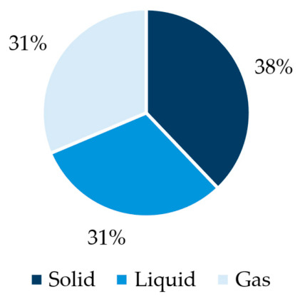
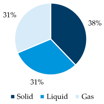
To develop and validate the proposed regression models, a database categorized by fuel state (solid, liquid, and gas) was compiled. The primary source of data was the NIST database [29]. However, as this database mainly contains gaseous and liquid fuels, additional solid-fuel data were collected from the BIOBIB and COALQUAL databases to improve the representation of solid fuels [30,31]. In total, 520 fuel samples were introduced, comprising 197 solids, 160 liquids, and 163 gases. The percentage distribution of samples by fuel state is presented in Figure 1.
Figure 1.
Samples distribution by state.
For each sample, the lower heating value (LHV) and elemental composition, including carbon (C), hydrogen (H), nitrogen (N), oxygen (O), and sulfur (S), were compiled into the database. Since ash does not contribute directly to fuel combustion, the regression models were developed considering only the organic fraction of the fuels. Accordingly, the elemental composition of solid fuels was converted to a dry ash-free (DAF) basis. Samples with sulfur contents above 5% were excluded, since elevated sulfur concentrations may promote equipment corrosion and increase pollutant emissions, making such fuels unsuitable for most conventional applications [32]. Consequently, the proposed correlations should not be extrapolated to high-sulfur fuels without additional validation.
In order to convert the elemental composition from dry basis into dry-ash-free basis, Equation (1) was applied:
where , are the mass fraction of the element in dry basis and dry-ash-free basis, respectively, and the is the mass fraction of ashes in dry basis. This conversion assumes that ash is inert and does not contribute to the combustible organic fraction.
The higher heating value (HHV) was not considered in this study, as latent heat recovery from water vapor condensation is generally not utilized in practical energy conversion systems. Therefore, the LHV was selected as the most representative heating value for the present investigation. Most of the data processing and organization procedures were carried out using Microsoft Excel®.
2.3. Model Development
2.3.1. Full Polynomial (FP) Model Formulation
Several models for predicting the LHV of fuels based on elemental composition can be found in the literature. However, different methodological approaches and parameter combinations have been proposed depending on the type of fuel and the intended application. In the present work, a correlation analysis was performed to evaluate the influence of the elemental composition parameters (C, H, N, O, and S) on the LHV of the samples. Based on this analysis, the three parameters showing the strongest correlation with LHV were selected for model development.
To describe both the individual contribution of each parameter and the interaction effects between variables, a second-degree polynomial model was adopted. The inclusion of interaction and quadratic terms allows the model to capture nonlinear relationships between elemental composition and LHV, which cannot be adequately represented using a purely linear formulation. Consequently, the proposed equation includes linear, quadratic, and cross-product terms, as can be noticed in Equation (2):
where , , and represent the elemental parameters selected from the correlation analysis. The coefficients to correspond to the regression constants obtained for each fuel category, differing for solid, liquid, and gaseous fuels.
The correlation analysis was initially conducted using Microsoft Excel®, since the database was originally compiled and organized in this environment. The corresponding results are presented in Table 2. Among the evaluated parameters, carbon, hydrogen, and oxygen exhibited the strongest correlations with LHV and were therefore selected for model development. Oxygen presented the highest absolute correlation coefficient (−0.844), indicating a strong inverse relationship with LHV, where increasing oxygen content reduces the fuel heating value. Carbon and hydrogen followed with positive correlation coefficients of 0.830 and 0.698, respectively, confirming their favorable contribution to fuel energy content. Sulfur and nitrogen exhibited comparatively lower correlations, with coefficients of −0.222 and −0.180, respectively. Although sulfur showed a moderate negative influence, its occurrence was primarily limited to solid fuels, being nearly absent in most liquid and gaseous samples. Notably, carbon and hydrogen were the only parameters presenting positive correlations with LHV.
Table 2.
Correlation analysis results.
Note that this correlation was performed for all the fuels at the same time, not distinguishing their state (solid, liquid, or gas).
From a physicochemical perspective, the positive influence of carbon and hydrogen is consistent with their dominant contribution to combustion energy, while oxygen generally reduces LHV because it represents a partially oxidized fraction of the fuel. Therefore, oxygen-rich fuels tend to present lower energy density. The interaction and polynomial terms should not be interpreted as direct combustion mechanisms, but as empirical descriptors of the nonlinear relationship between elemental composition and heating value across chemically diverse fuels.
As a next step, Equation (2) was updated by replacing , , and with the three parameters identified as most influential: Carbon, Hydrogen, and Oxygen, respectively.
Following this update, the Python code was executed to determine the corresponding coefficients for each fuel type. The resulting equation is presented in Equation (3):
where , , are the mass fractions of DAF of carbon, hydrogen, and oxygen from each sample.
The terms , , correspond to the squared values of the respective elemental contents. The terms , , and are mathematical interaction terms obtained by multiplying the corresponding elemental contents. These polynomial and interaction terms are empirical regression variables and should not be interpreted as chemical species, molecular bonds, or reaction products. To avoid ambiguity, the interaction terms are written using the multiplication symbol throughout the manuscript.
To determine the regression coefficients ( to ), a Python 3.12 code was developed using the LinearRegression estimator from the scikit-learn 1.9 library [33]. The database was first separated according to fuel state, namely solid, liquid, and gaseous fuels, and an independent regression was performed for each group. The LinearRegression estimator applies ordinary least squares regression, minimizing the residual sum of squares between the experimental and predicted LHVs. The complete dataset of each fuel state was used to estimate the final coefficients reported in this work. This step corresponds to the final calibration of the proposed equations and was performed because the objective of the study was to provide deployable correlations for subsequent engineering use.
It is important to distinguish this final calibration step from the model validation procedure. The full-dataset coefficients define the final calibrated equations, but they were not used as the sole basis for assessing predictive generalization. Model robustness and predictive capability were evaluated separately using the 10-fold cross-validation procedure described in Section 2.5. In this procedure, the coefficients were recalculated independently using only the training folds, and the prediction errors were computed using the corresponding unseen testing fold. Table 3 resumes the parameters used for this model.
Table 3.
Final calibration parameters for coefficient estimation.
The parameters used for the final full-dataset calibration are summarized in Table 3, while the independent cross-validation procedure used for model evaluation is summarized separately in Table 4.
Table 4.
Cross-validation parameters for model validation.
The code is designed to automatically extract information from the database, divide the data into groups based on state, and perform a separate linear regression for each group. Once the regression coefficients are determined, they are exported to a text file, which can be easily imported into any spreadsheet. To update the coefficients, the user simply needs to update the database and run the code.
2.3.2. Multicollinearity Assessment (VIF)
Since the proposed correlation includes linear, quadratic, and interaction terms, the possibility of multicollinearity between predictors was evaluated. As stated by Kim [12], in regression-based models, multicollinearity occurs when two or more variables exhibit strong linear dependence, potentially leading to unstable regression coefficients, reduced interpretability, and excessive sensitivity of the model to small variations in the dataset. This effect is particularly relevant in second-degree polynomial formulations, where quadratic and cross-product terms may contain overlapping information. To assess the degree of parameter redundancy, the Variance Inflation Factor (VIF) was calculated for each predictor. The VIF quantifies the extent to which the variance of a regression coefficient is increased due to correlations with the remaining predictors. In general, elevated VIF values indicate excessive collinearity and suggest that the corresponding variable may not contribute independently to the model formulation. Based on the VIF analysis, the complete polynomial formulation was evaluated regarding parameter redundancy and statistical stability. The results of the VIF are presented in the Section 3.5 of this paper. Parameters exhibiting excessive multicollinearity were subsequently assessed for removal in order to obtain a simplified formulation with improved robustness and interpretability while maintaining satisfactory predictive performance.
2.3.3. Simplified Polynomial (SP) Model Development
After the development of the FP model, the multicollinearity between the independent variables was evaluated using the VIF. The analysis revealed that several second-order and interaction terms exhibited high VIF values, indicating strong linear dependence between predictors. Since multicollinearity inflates the variance of regression coefficients and may compromise the statistical reliability and physical interpretability of the model, a simplification procedure was carried out.
Based on the VIF analysis, the terms C2, H2, O2, and HO were removed from the original formulation. These variables presented significant redundancy with the remaining predictors, particularly due to the strong interaction already represented by the CH and CO terms. In addition, the quadratic terms showed strong correlation with their respective linear variables, contributing to unstable coefficient estimation and unnecessary model complexity.
The resulting Simplified Polynomial (SP) model is presented in Equation (4):
The simplified formulation preserves the main interaction effects between the elemental composition variables while substantially reducing multicollinearity. Furthermore, the removal of statistically redundant terms allows a more physically interpretable equation, reducing the risk of overfitting while maintaining predictive capability. Similar approaches have been reported in regression-based calorific value prediction studies, where simplified models often provide improved generalization performance compared to highly parameterized polynomial formulations [10,18].
The predictive performance of the SP model was subsequently evaluated and compared with the FP model.
2.4. Error Metrics
To evaluate the predictive accuracy and robustness of the proposed model, several statistical error metrics commonly reported in the literature were considered [21]. Since a single metric may not fully describe model performance, multiple complementary indicators were considered to assess both the magnitude and the distribution of prediction errors. Eight statistical parameters were selected for this purpose: maximum deviation between experimental and predicted values, coefficient of determination (R2), Mean Absolute Error (MAE), Mean Squared Error (MSE), Root Mean Square Error (RMSE), Mean Absolute Percentage Error (MAPE), Symmetric Mean Absolute Percentage Error (sMAPE), and bias. These metrics evaluate complementary aspects of predictive performance, including average error magnitude, sensitivity to large deviations, relative percentage errors, and systematic prediction tendencies. The last six parameters are presented in Equations (5)–(10)
In these equations, the subscripts and denote experimental and predicted LHVs, respectively. The combined use of multiple statistical indicators provides a more comprehensive assessment of model performance, reducing the risk of biased conclusions based on a single error criterion.
2.5. Cross-Validation Methodology
To ensure that the proposed equations were not overfit to the specific dataset used for coefficient determination, a cross-validation procedure was applied to evaluate the robustness and generalization capability of the developed models. Cross-validation allows the predictive performance of a model to be assessed using unseen data, providing a more reliable estimation of its applicability.
The cross-validation analysis was implemented using the Python language with the Scikit-learn library. The KFold function from the Sklearn module was used to perform the data partitioning procedure, while the regression calculations were carried out using the LinearRegression function from the Sklearn module. Initially, the complete dataset was randomly shuffled to minimize potential bias associated with the original sample ordering. Subsequently, the dataset was divided into approximately equal subsets (folds). During each iteration, that one fold was used as the testing dataset, and the remaining folds were used for model training [34]. This procedure was repeated until all folds had been used once as testing data.
In the present work, a 10-fold cross-validation approach was adopted. Consequently, for each iteration, approximately 90% of the data were used for model training and 10% for testing. The regression coefficients were recalculated independently for every iteration, allowing the evaluation of model stability and sensitivity to variations in the training dataset.
Table 4 summarizes the main parameters adopted in the cross-validation procedure. The predictive performance was evaluated using the statistical metrics previously presented. The adopted methodology ensures that the predictive capability of the equations is not assessed using the same data employed for coefficient determination, reducing the risk of overfitting and providing a more realistic estimation of model performance for unseen datasets.
3. Validation and Application
3.1. Coefficient Determination
The regression coefficients of the proposed models were obtained through multiple linear regression analysis using the datasets corresponding to the solid, liquid, and gaseous fuel states. Independent regressions were performed for each physical state to account for the distinct thermochemical behavior and elemental distribution observed between fuel classes.
Table 5 presents the coefficients obtained for the FP model. Due to the inclusion of linear, quadratic, and interaction terms, the FP formulation required a larger number of coefficients to represent the nonlinear relationships between the elemental composition variables and the LHV. The obtained coefficients varied significantly between fuel states, highlighting the different sensitivities of solid, liquid, and gaseous fuels to the elemental interactions considered in the model.
Table 5.
Coefficients obtained for the FP model.
The coefficients associated with the quadratic and interaction terms showed considerable magnitude variations, particularly for gaseous fuels, indicating stronger nonlinear effects within this dataset. However, as discussed previously in the VIF analysis, several of these terms contributed to increased multicollinearity, reducing the statistical stability of the regression model.
To reduce multicollinearity, a simplified formulation was subsequently developed by removing the statistically redundant terms identified during the VIF assessment. The resulting coefficients for the SP model are presented in Table 6.
Table 6.
Coefficients obtained for the SP model.
Compared with the FP model, the SP equation required fewer coefficients while preserving the main interaction effects between the elemental variables. The simplified formulation also produced coefficients with improved numerical stability and physical interpretability.
The differences observed between the coefficients for solids, liquids, and gases reinforce the importance of separating the datasets according to physical state, since the influence of carbon, hydrogen, oxygen, and their interactions on the calorific value is not identical across all fuel types.
3.2. Performance Analysis
As shown previously in Table 2, the correlation proposed by Mollanoori et al. [16] and Channiwala et al. [17] was originally developed for HHV estimation. However, the present work focuses on a model for LHV estimation. Therefore, the Equations proposed in the literature were adapted based on Hosokay et al.’s [8] work. Noticing that, LHV can be obtained by the HHV by removing the latent heat associated with water vaporization. The adapted equation follows Equation (11):
where is the mass fraction of hydrogen in the DAF basis of the sample, and are the molar masses of water and hydrogen, respectively, and the 2.4 represents the latent heat of vaporization of water. After this conversion, the adapted literature equations were evaluated using the same statistical methodology applied to the proposed models.
The results of the performance metrics are presented in Table 7. As can be observed, the results demonstrate that the proposed regression models outperformed the literature correlations for the prediction of LHV across the analyzed dataset. Among all evaluated equations, the FP model exhibited the best overall predictive performance, presenting the lowest values for Max Deviation (8.9 MJ/kg), MAE (1.06 MJ/kg), MSE (2.37 MJ2/kg2), RMSE (1.54 MJ/kg), MAPE (4.85%), and sMAPE (5.99%), together with the highest coefficient of determination (). These results indicate excellent agreement between predicted and experimental values and confirm the high fitting capability of the complete polynomial formulation.
Table 7.
Performance metrics of the developed literature models.
The SP model also showed strong predictive capability, with only a slight reduction in accuracy compared to the FP model. Although the SP equation presented moderately higher errors, the differences remained relatively small, particularly considering the reduction in model complexity after removing multicollinear terms. The increase in RMSE from 1.54 MJ/kg to 1.63 MJ/kg and the reduction of from 0.99 to 0.98 indicates that the simplification procedure preserved most of the predictive capability of the original formulation.
The literature models presented considerably larger deviations and error values. The Hosokai equation showed the highest maximum deviation (35.30 MJ/kg), indicating limited capability to represent extreme fuel compositions present in the dataset. Similarly, the Channiwala, Boie, and Mollanoori correlations produced larger MAE, RMSE, and percentage-based errors when compared with the proposed models. These differences can be attributed to the fact that most literature correlations were developed using more restricted datasets, often focused on specific fuel classes such as coal, biomass, or conventional fossil fuels, limiting their applicability to highly heterogeneous datasets containing solid, liquid, and gaseous fuels simultaneously.
Regarding the bias values, both the FP and SP models presented values close to zero, indicating the absence of systematic overprediction or underprediction tendencies. In contrast, some literature models exhibited noticeable positive or negative bias, suggesting systematic deviations depending on the fuel composition.
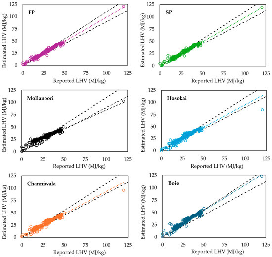
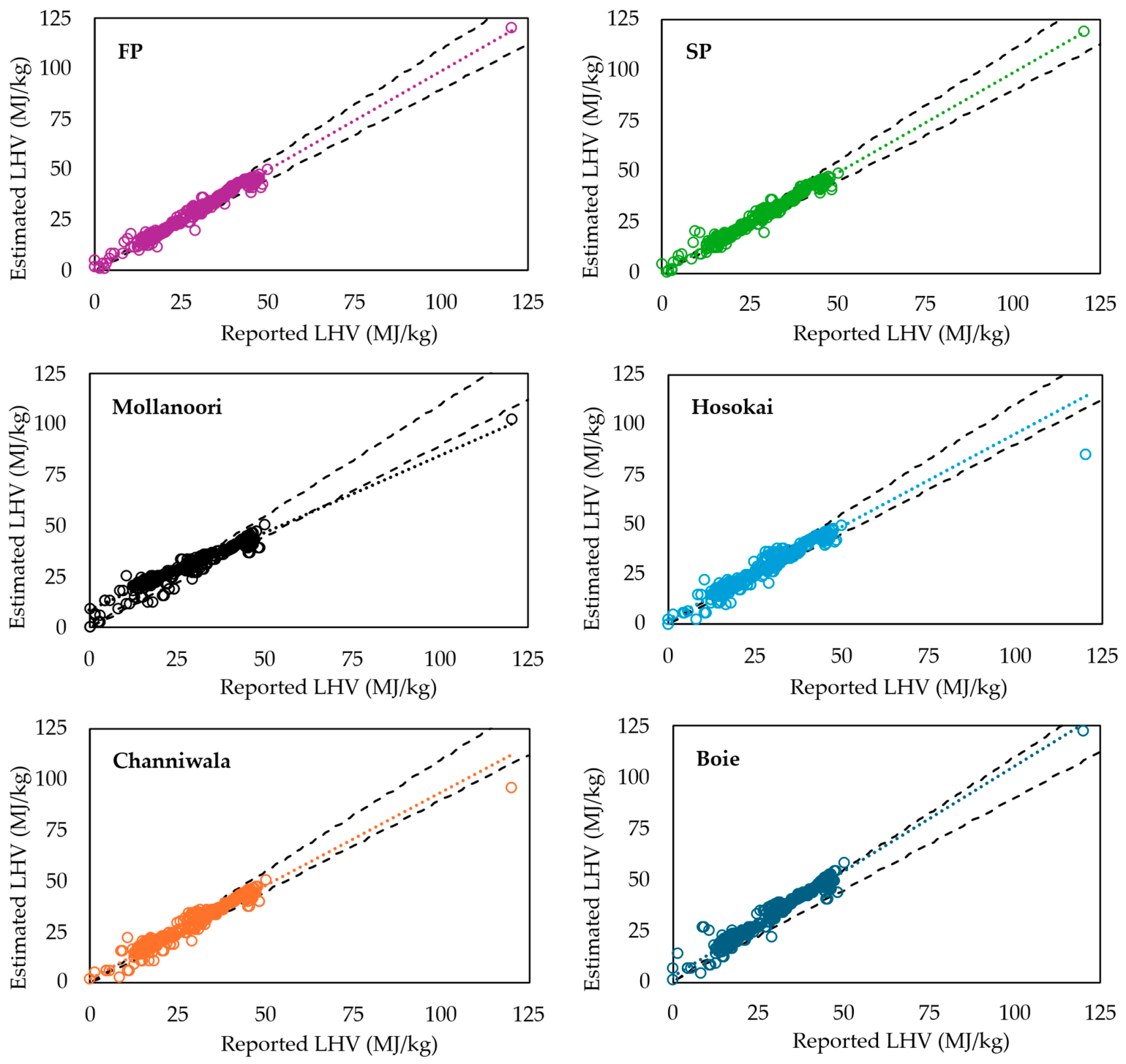
The predicted-versus-reported LHV plots presented in Figure 2 provide a visual assessment of the predictive capability of the proposed and literature models. In all cases, the dashed central line represents the ideal condition where predicted and experimental values are identical, while the outer dashed lines represent the 10% error limits adopted for visualization purposes.
Figure 2.
Predicted vs. experimental LHVs for the proposed models and the literature ones [8,15,16,17]. The colored dashed line represents the fitted trend line for each model, while the black dashed lines indicate the ±10% error.
The proposed FP and SP models showed the best agreement with the experimental data (also in accordance with the R2 results), with most points concentrated near the ideal prediction line throughout the entire LHV range. The FP model exhibited the smallest dispersion, confirming the superior statistical indicators previously presented. The SP model showed slightly larger deviations, particularly at higher LHVs, but still maintained a strong correlation between predicted and reported values. These results indicate that the simplification process reduced model complexity while preserving most of the predictive capability.
The literature equations presented visibly larger deviations and data dispersion. The Mollanoori et al. [16] and Hosokai et al. [8] correlations tended to underestimate high LHV fuels, while the Channiwala et al. [17] and Boie et al. [15] models exhibited larger scatter for low and intermediate LHV samples. A common feature observed in all models is the presence of a significant outlier located at very high reported LHVs. This point corresponds to the hydrogen-rich gaseous fuel sample (), which presents an exceptionally high LHV compared to the remaining dataset. Due to its extreme elemental composition, particularly the very high hydrogen content and absence of carbon, this sample lies outside the main compositional domain represented by the other fuels. Consequently, all evaluated models exhibited increased prediction deviations for this specific case.
Nevertheless, the H2 sample was intentionally maintained in the database to ensure that the developed equations were exposed to extreme fuel compositions and to avoid restricting their applicability only to conventional hydrocarbon fuels. To evaluate its influence, a sensitivity analysis was performed for the gaseous-fuel subset. The FP and SP models were calibrated and evaluated under two conditions: first, using the complete gaseous-fuel database, including H2, and then after excluding the H2 sample, with the coefficients recalculated for the reduced database. The results, summarized in Table 8, show that the exclusion of H2 produced only minor changes in the global predictive metrics. These results indicate that, although H2 represents an extreme compositional point and contributes to the graphical spread of the gaseous-fuel dataset, it does not substantially distort the global predictive performance of the proposed models.
Table 8.
Sensitivity analysis of the gaseous-fuel models with and without the pure H2 sample.
The H2 sample was therefore retained in the final database because hydrogen-rich fuels are increasingly relevant in modern energy applications and because their inclusion provides a stricter test of model applicability. Nevertheless, prediction errors for pure hydrogen and highly hydrogen-enriched mixtures should be interpreted carefully, and dedicated sub-models may provide improved accuracy for applications focused specifically on this fuel class. Although this point increases the overall deviation metrics and graphical dispersion at high LHVs, its inclusion provides a more rigorous evaluation of model robustness and generalization capability.
The statistical results demonstrate that the proposed regression formulations provide a favorable and accurate equation for the LHV estimation. In particular, the SP guarantees a balance between predictive accuracy and mathematical simplicity. The graphical analysis demonstrates that the proposed polynomial formulations provide improved predictive performance and better adaptability to a broad range of fuel compositions compared with the literature correlations.
Although the improvement in the coefficient of determination was moderate compared with some literature correlations, the proposed models provided a more consistent improvement across complementary error metrics. This distinction is important because a high R2 alone does not necessarily ensure low prediction error for individual fuels. In thermochemical process modeling, errors in LHV estimation may propagate into energy balances, efficiency calculations, fuel selection, and preliminary design assumptions. Thus, the practical contribution of the proposed correlations lies in reducing the expected prediction error and improving the reliability of LHV estimates across solid, liquid, and gaseous fuels within the validated compositional domain.
3.3. Bland–Altman Analysis
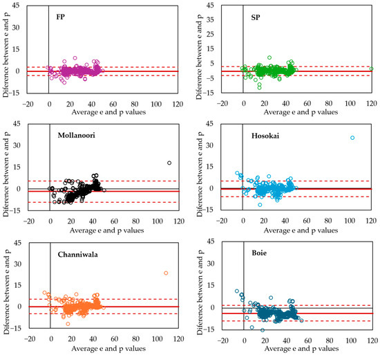
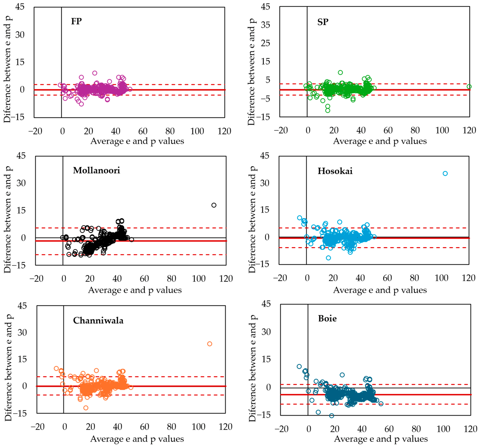
The Bland–Altman plots presented in Figure 3 were used to evaluate the agreement between the reported and predicted LHVs for the proposed and literature models. In these plots, the central solid line represents the mean bias, while the dashed lines correspond to the limits of agreement (LoA), defined as the bias ± 1.96 standard deviations.
Figure 3.
Bland–Altman analysis comparing predicted and reported LHVs for the proposed models and selected literature [8,15,16,17]. The solid red line represents the mean bias, the red dashed lines indicate the 95% limits of agreement.
The proposed FP and SP models exhibited the best agreement with the experimental data. Both models presented biases very close to zero, indicating the absence of systematic overestimation or underestimation tendencies. The FP model showed a bias of 0.00 MJ/kg with limits of agreement between −3.02 and +3.02 MJ/kg, while the SP model presented similarly narrow limits between −3.20 and +3.20 MJ/kg. Additionally, most data points were densely concentrated around the zero-difference line, demonstrating high consistency and low dispersion across the analyzed LHV range.
The literature models showed noticeably wider limits of agreement and larger systematic deviations. The Hosokai et al. [8] model presented a small negative bias (−0.37 MJ/kg), although the dispersion increased considerably due to the presence of the hydrogen fuel sample, reaching the limits between −5.93 MJ/kg and 5.20 MJ/kg. The Channiwala et al. [17] model exhibited a slight positive bias (0.35 MJ/kg) but larger LoA than the proposed models, with lower and upper limits of −4.85 MJ/kg and 5.55 MJ/kg. The Mollanoori et al. [16] correlations presented a negative bias (−1.72 MJ/kg), indicating systematic underprediction tendencies for the analyzed dataset, with the lower and upper limits of −9.15 MJ/kg and 7.71 MJ/kg, being the model with the widest interval of the LoA. The Boie et al. [15] model was the one that exhibited the lowest bias, with a value of −3.61 MJ/kg and with limits of agreement ranging from −8.90 MJ/kg to 1.68 MJ/kg, demonstrating both higher dispersion and asymmetric prediction behavior. This asymmetry suggests that the equation tends to systematically underestimate the LHV, particularly for higher-energy fuels.
A common characteristic observed in all literature models is the presence of an extreme outlier corresponding to the hydrogen fuel (as exhibited previously in the predicted vs. experimental graphs). Due to its exceptionally high LHV and atypical elemental composition, this sample strongly influences the agreement limits and increases the overall dispersion, particularly for the Hosokai et al. [8] and Channiwala et al. [17] correlations.
3.4. Cross-Validation—FP vs. SP
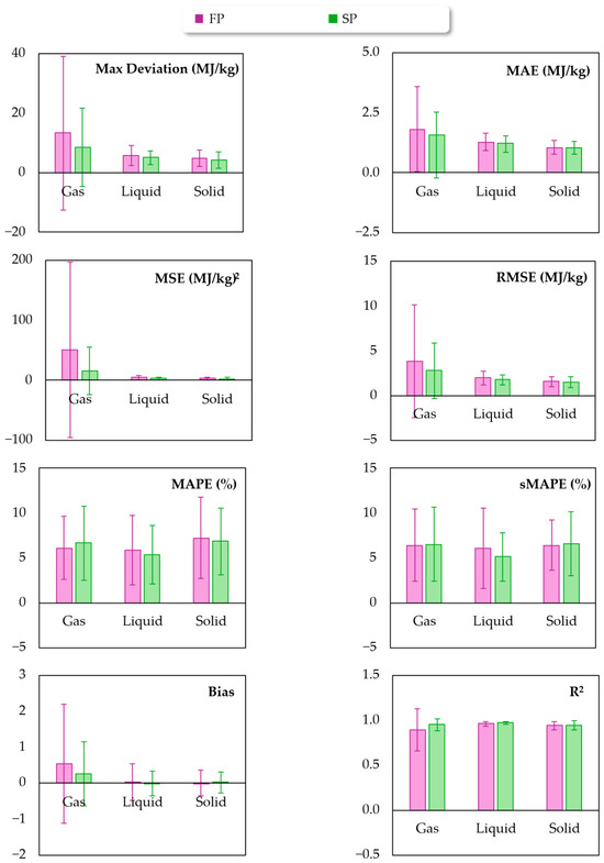
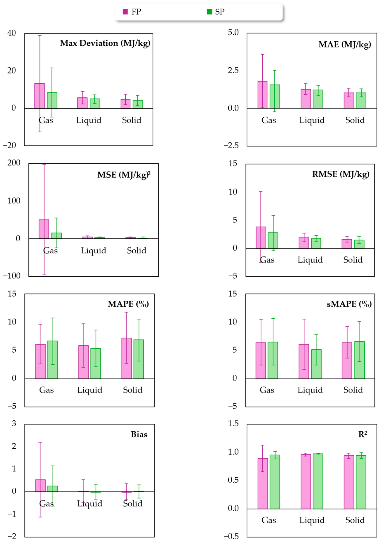
The robustness analysis presented in Figure 4 compares the predictive stability of the FP and SP models using the statistical metrics previously studied and obtained through the cross-validation procedure.
Figure 4.
Cross-validation analysis performed for the FP and SP.
Both models demonstrated high predictive robustness, with relatively small variations in the evaluated statistical metrics between cross-validation iterations. However, the results also reveal important differences regarding model stability and generalization capability.
As observed in Figure 4, the SP model generally presented lower average cross-validation errors than the FP model, except for the MAPE values for gaseous fuels and the sMAPE values for gaseous and solid fuels. Additionally, the FP formulation exhibited noticeably larger standard deviations, particularly for gaseous fuels, especially where the hydrogen sample was not included in the training dataset. This behavior is particularly evident in the Max Deviation, MSE, RMSE, and Bias metrics, where the dispersion associated with the gaseous dataset became substantially higher. The increased variability indicates that the FP model is more sensitive to the redistribution of samples between training and testing subsets during cross-validation. Such sensitivity is expected due to the larger number of regression coefficients and the presence of multicollinearity.
In contrast to the FP model that provided superior fitting performance when evaluated using the complete dataset, the SP model generally produced lower variability during cross-validation, indicating improved robustness and reduced sensitivity to sample redistribution. This effect is particularly relevant for gaseous fuels, where the presence of hydrogen strongly influences the regression process.
The R2 values demonstrate that both formulations remained consistently high for all fuel states, typically above 0.90, confirming that the simplification procedure did not significantly compromise the predictive capability of the model. The close agreement between the FP and SP R2 values further demonstrates that most of the predictive information was preserved after removing the multicollinear terms.
While the FP model achieved the best overall fitting performance, the SP formulation demonstrated a more favorable balance between predictive accuracy and robustness when evaluated under unseen data conditions.
3.5. Multicollinearity Results
Table 9 presents the VIF values obtained for the FP and SP formulations for gaseous, liquid, and solid fuels. The VIF analysis was performed to evaluate the degree of multicollinearity between the independent variables used in the regression models [12].
Table 9.
Results for the VIF for the FP and SP models.
The FP model exhibited extremely high VIF values for most variables and fuel states, particularly for the linear terms C, H, and O, as well as for the quadratic terms C2 and O2. The highest values were observed for the solid fuel dataset, where the VIF associated with O reached 2459.8. Nevertheless, high values were also observed for the gaseous and liquid datasets.
These results indicate severe multicollinearity within the FP model. According to the literature, VIF values above 10 already indicate collinearity between predictors, leading to inflated variances of the regression coefficients and reduced statistical reliability of the model. Therefore, the VIF values observed for the FP model demonstrate that several variables were strongly linearly dependent, particularly due to the simultaneous inclusion of linear, quadratic, and interaction terms derived from the same elemental variables [12].
Considering the VIF of each parameter, and after testing several combinations throughout all datasets, the one that best comprised the VIF values with the statistical method was the SP that was obtained by simply starting with the FM as a base and removing the C2, H2, O2, and HO parameters.
The SP model presented a substantial reduction in multicollinearity. The VIF values decreased considerably for all fuel states, confirming that the removed variables were major contributors to the collinearity problem. The largest reductions were observed for the gaseous and liquid datasets, where several parameters had a reduction above 90%.
Despite the substantial improvement, some variables still presented moderately elevated VIF values in the SP formulation, particularly for the solid fuels dataset. This behavior is expected due to the intrinsic correlation between elemental compositions in fuel samples, especially between carbon and oxygen contents. Nevertheless, the obtained values represent a significant improvement in comparison with the original formulation and are consistent with the improved stability observed during the cross-validation analysis.
Although the simplified polynomial formulation substantially reduced multicollinearity, some moderate collinearity remained due to the inherent dependence between elemental composition variables. Regularized regression approaches, such as ridge regression or elastic net regression, may further improve coefficient stability and are recommended as future refinements. However, the present study retained the simplified polynomial model because it provides an explicit equation suitable for direct engineering use.
4. Conclusions
This study developed and validated generalized regression-based models for estimating the LHV of fuels from ultimate analysis data. By using a broad database containing 520 fuels, divided into solid, liquid, and gaseous states, the proposed formulations demonstrated that elemental composition alone could provide reliable estimations of fuel energy content across a wide range of fuel classes.
The F.P. model achieved the highest overall predictive capability, confirming the benefit of incorporating second-order and interaction terms to capture the nonlinear influence of carbon, hydrogen, and oxygen on the heating value. However, the multicollinearity assessment revealed that several polynomial terms introduced strong linear dependencies, increasing the variance of regression coefficients and reducing model robustness.
A SP model was developed by removing from the FP statistically redundant terms identified through the multicollinearity analysis. The resulting equation preserved the second-order structure while substantially improving the statistical consistency of the regression coefficients. Although the SP model produced slightly lower fitting performance on the complete dataset, the cross-validation results demonstrated improved robustness and generalization capability, indicating reduced sensitivity to data partitioning and lower risk of overfitting.
The comparison with literature correlations further highlighted the relevance of the proposed models. The proposed equations showed competitive or superior predictive performance across multiple error metrics, confirming the importance of incorporating nonlinear interactions when attempting to describe a generalized fuel database.
The Bland–Altman analysis additionally demonstrated that the developed models presented limited systematic bias and acceptable agreement between predicted and measured values over the entire LHV range.
Although 10-fold cross-validation provides evidence of internal predictive robustness, an independent, blind external validation dataset would further strengthen the assessment of model generalization.
The proposed correlations provide a practical compromise between predictive accuracy, statistical robustness, and applicability to different fuel types.
Although the proposed models were developed using a broad database including solid, liquid, and gaseous fuels, their applicability remains bounded by the composition range of the training dataset and by the selected modeling variables. In particular, the present correlations were derived using C, H, and O as primary predictors because these variables showed the strongest correlation with LHV in the compiled dataset (as stated in Section 2.3.1). Therefore, fuels with unusually high nitrogen or sulfur contents, highly specific molecular structures, or extreme elemental compositions should be interpreted with caution. The proposed equations should be regarded as practical engineering correlations for preliminary LHV estimation rather than universal replacements for experimental calorimetry.
Author Contributions
Conceptualization, C.C.; methodology, C.C.; software, C.C.; validation, C.C., N.P. and J.C.T.; formal analysis, C.C. and M.G.; investigation, C.C. and N.P.; data curation, C.C.; writing—original draft preparation, C.C. and N.P.; writing—review and editing, C.C., N.P. and J.C.T.; supervision, M.G. and J.C.T. All authors have read and agreed to the published version of the manuscript.
Funding
This work was supported by FCT—Fundação para a Ciência e Tecnologia through the PhD Grant (2023.01517.BD), the MEtRICs research unit (UID/04077/2025), and the VALORIZA research unit (UID/05064/2025 and by national funds from FCT, under the scope of the projects UID/50006/2025, UID/PRR/50006/2025 and LA/P/0008/2020 of the Associated Laboratory for Green Chemistry—LAQV REQUIMTE).
Institutional Review Board Statement
Not applicable.
Informed Consent Statement
Not applicable.
Data Availability Statement
The original contributions presented in this study are included in the article. Further inquiries can be directed to the corresponding author.
Conflicts of Interest
The authors declare no conflicts of interest.
Abbreviations
The following abbreviations are used in this manuscript:
| C | Carbon |
| DAF | Dry Ash-Free |
| FP | Full Polynomial Model |
| H | Hydrogen |
| HHV | Higher Heating Value |
| LHV | Lower Heating Value |
| MAE | Mean Absolute Error |
| MAPE | Mean Absolute Percentage Error |
| MSE | Mean Squared Error |
| N | Nitrogen |
| O | Oxygen |
| RDF | Refuse Derived Fuel |
| RMSE | Root Mean Square Error |
| S | Sulfur |
| sMAPE | Symmetric Mean Absolute Percentage Error |
| SP | Simplified Polynomial Model |
| VIF | Variance Inflation Factor |
| Subscripts and Superscripts | |
| e | experimental |
| p | predicted |
References
- Varjani, S.; Shahbeig, H.; Popat, K.; Patel, Z.; Vyas, S.; Shah, A.V.; Barceló, D.; Ngo, H.H.; Sonne, C.; Lam, S.S.; et al. Sustainable management of municipal solid waste through waste-to-energy technologies. Bioresour. Technol. 2022, 355, 127247. [Google Scholar] [CrossRef] [Scilit] [PubMed]
- Lombardi, L.; Carnevale, E.; Corti, A. A review of technologies and performances of thermal treatment systems for energy recovery from waste. Waste Manag. 2015, 37, 26–44. [Google Scholar] [CrossRef] [Scilit] [PubMed]
- Çengel, Y.A.; Boles, M.A.; Kanoglu, M. Thermodynamics an Engineering Approach, 9th ed.; McGraw-Hill Education: New York, NY, USA, 2019. [Google Scholar]
- Li, Z.B.; Yu, Y.; Jia, L.; Wu, Y.W.; Cheng, P.; Zhang, Z.; Li, Z.K.; Fan, C.H.; Guo, X.M. Thermal characteristic analysis and performance optimization of a novel heating boiler based on a porous media model. Appl. Therm. Eng. 2026, 289, 130035. [Google Scholar] [CrossRef] [Scilit]
- Esteves, B.; Sen, U.; Pereira, H. Influence of Chemical Composition on Heating Value of Biomass: A Review and Bibliometric Analysis. Energies 2023, 16, 4226. [Google Scholar] [CrossRef] [Scilit]
- Sheng, C.; Azevedo, J.L.T. Estimating the higher heating value of biomass fuels from basic analysis data. Biomass Bioenergy 2005, 28, 499–507. [Google Scholar] [CrossRef] [Scilit]
- Demirbas, A.; Gullu, D.; Çaglar, A.; Akdeniz, F. Estimation of calorific values of fuels from lignocellulosics. Energy Sources 1997, 19, 765–770. [Google Scholar] [CrossRef] [Scilit]
- Hosokai, S.; Matsuoka, K.; Kuramoto, K.; Suzuki, Y. Modification of Dulong’s formula to estimate heating value of gas, liquid and solid fuels. Fuel Process. Technol. 2016, 152, 399–405. [Google Scholar] [CrossRef] [Scilit]
- Erdoğan, S. LHV and HHV prediction model using regression analysis with the help of bond energies for biodiesel. Fuel 2021, 301, 121065. [Google Scholar] [CrossRef] [Scilit]
- Mateus, M.M.; Bordado, J.M.; Santos, R.G.D. Simplified multiple linear regression models for the estimation of heating values of refuse derived fuels. Fuel 2021, 294, 120541. [Google Scholar] [CrossRef] [Scilit]
- Ozyuguran, A.; Akturk, A.; Yaman, S. Optimal use of condensed parameters of ultimate analysis to predict the calorific value of biomass. Fuel 2018, 214, 640–646. [Google Scholar] [CrossRef] [Scilit]
- Kim, J.H. Multicollinearity and misleading statistical results. Korean J. Anesthesiol. 2019, 72, 558–569. [Google Scholar] [CrossRef] [Scilit] [PubMed]
- Mansournia, M.A.; Waters, R.; Nazemipour, M.; Bland, M.; Altman, D.G. Bland-Altman methods for comparing methods of measurement and response to criticisms. Glob. Epidemiol. 2021, 3, 100045. [Google Scholar] [CrossRef] [Scilit] [PubMed]
- Clarke Energy. LHV vs. HHV in Data Centers: Why Fuel Definitions Matter for Onsite Power Economics. Available online: https://www.clarke-energy.com/2026/lhv-vs-hhv-in-data-centers-why-fuel-definitions-matter-for-onsite-power-economics/ (accessed on 14 April 2026).
- Ringen, S.; Lanum, J.; Miknis, F.P. Calculating heating values from elemental composition of fossil fuels. Fuel 1979, 58, 69–71. [Google Scholar] [CrossRef] [Scilit]
- Mollanoori, M.; Dehghan, A.A. Estimating the higher heating value and chemical exergy of solid, liquid, and natural gas fossil fuels. Energy 2024, 302, 131835. [Google Scholar] [CrossRef] [Scilit]
- Channiwala, S.A.; Parikh, P.P. A unified correlation for estimating HHV of solid, liquid and gaseous fuels. Fuel 2002, 81, 1051–1063. [Google Scholar] [CrossRef] [Scilit]
- Friedl, A.; Padouvas, E.; Rotter, H.; Varmuza, K. Prediction of heating values of biomass fuel from elemental composition. Anal. Chim. Acta 2005, 544, 191–198. [Google Scholar] [CrossRef] [Scilit]
- Cooper, C.D.; Kim, B.; MacDonald, J. Estimating the lower heating values of hazardous and solid wastes. J. Air Waste Manag. Assoc. 1999, 49, 471–476. [Google Scholar] [CrossRef] [Scilit] [PubMed]
- Mehta, P.S.; Anand, K. Estimation of a lower heating value of vegetable oil and biodiesel fuel. Energy Fuels 2009, 23, 3893–3898. [Google Scholar] [CrossRef] [Scilit]
- Özyuğuran, A.; Yaman, S.; Küçükbayrak, S. Prediction of calorific value of biomass based on elemental analysis. Int. Adv. Res. Eng. J. 2018, 2, 254–260. [Google Scholar]
- Demirbas, A. Calculation of higher heating values of biomass fuels. Fuel 1997, 76, 431–434. [Google Scholar] [CrossRef] [Scilit]
- Xie, Y.; Yan, H.; Dong, C.; Xue, J.; Zhang, J.; Hu, X. Research on the LHV prediction for biomass fuel based on near-infrared spectroscopy and local model strategy. Biomass Bioenergy 2026, 208, 108832. [Google Scholar] [CrossRef] [Scilit]
- García, P.J.; García, E.; Paredes, J.P. Estimation of the coal higher heating value for energy systems relied on ultimate analysis with machine learning techniques. Fuel 2024, 357, 130037. [Google Scholar] [CrossRef] [Scilit]
- Yaka, H.; Insel, M.A.; Yucel, O.; Sadikoglu, H. A comparison of machine learning algorithms for estimation of higher heating values of biomass and fossil fuels from ultimate analysis. Fuel 2022, 320, 123971. [Google Scholar] [CrossRef] [Scilit]
- Insel, M.A.; Yucel, O.; Sadikoglu, H. Higher heating value estimation of wastes and fuels from ultimate and proximate analysis by using artificial neural networks. Waste Manag. 2024, 185, 33–42. [Google Scholar] [CrossRef] [Scilit] [PubMed]
- Reddy, M.S.; Basha, S.; Joshi, H.V.; Kumar, V.G.S.; Jha, B.; Ghosh, P.K. Modeling the energy content of combustible ship-scrapping waste at Alang-Sosiya, India, using multiple regression analysis. Waste Manag. 2005, 25, 747–754. [Google Scholar] [CrossRef] [Scilit] [PubMed]
- Wang, D.; Tang, Y.T.; He, J.; Yang, F.; Robinson, D. Generalized models to predict the lower heating value (LHV) of municipal solid waste (MSW). Energy 2021, 216, 119279. [Google Scholar] [CrossRef] [Scilit]
- Burgess, D.R., Jr.; Hamins, A.P. Heats of Combustion and Related Properties of Pure Substances; National Institute of Standards and Technology: Gaithersburg, MD, USA, 2023. [CrossRef] [Scilit]
- Reisinger, K.; Haslinger, C.; Herger, M.; Hofbauer, H. BIOBIB—A Database for Biofuels; Institute of Chemical Engineering, Fuel and Environmental Technology, University of Technology Vienna: Vienna, Austria, 1996; Available online: http://cdmaster2.vt.tuwien.ac.at/biobib/info.html (accessed on 10 January 2025).
- Palmer, C.A.; Oman, C.L.; Park, A.J.; Luppens, J.A. The U.S. Geological Survey Coal Quality (COALQUAL) Database Version 3.0. Available online: http://ncrdspublic.er.usgs.gov/coalqual/ (accessed on 7 May 2025).
- Niu, X.; Wang, Y.; Liu, H.; Li, X.; Duan, L. The impact of chlorine and sulfur on alkali metal migration and submicron particle formation during solid fuel combustion. J. Energy Inst. 2024, 114, 101588. [Google Scholar] [CrossRef] [Scilit]
- Scikit-Learn. LinearRegression. Available online: https://scikit-learn.org/stable/modules/generated/sklearn.linear_model.LinearRegression.html (accessed on 10 January 2025).
- Scikit-Learn. KFold. Available online: https://scikit-learn.org/stable/modules/generated/sklearn.model_selection.KFold.html (accessed on 11 May 2026).

Disclaimer/Publisher’s Note: The statements, opinions and data contained in all publications are solely those of the individual author(s) and contributor(s) and not of MDPI and/or the editor(s). MDPI and/or the editor(s) disclaim responsibility for any injury to people or property resulting from any ideas, methods, instructions or products referred to in the content. |
© 2026 by the authors. Licensee MDPI, Basel, Switzerland. This article is an open access article distributed under the terms and conditions of the Creative Commons Attribution (CC BY) license.