


Abstract
The features of non-destructive testing of steel pipes with a long service life in terms of dynamic hardness parameters are considered. Regarding the limited applicability of normal and lognormal distributions, the Weibull and Gumbel distributions are used to describe the distribution density of hardness estimates for steels that have been in long-term operation in harsh meteorological and functional conditions. A number of experiments were carried out on the formation of digital images of the hardness distribution over the surface of the tested products. Hypotheses were formulated regarding the use of such images to assess the current technical state of metal products and the dynamics of its change. The possibility of describing the hardness of steel specimens used for a long time in difficult conditions by a weighted sum of two normal distributions has been experimentally proven.
1. Introduction
One of the most important characteristics of oil, natural gas, and hydrogen pipeline transport systems is their durability [1,2,3,4]. Special steels continue to be the main material for high-pressure trunk pipelines [5,6,7,8]. The reliability of a technical product of any degree of complexity is laid down at the stages of its design, manufacture, assembly, and checkout [9]. With regard to the control objects (CO) under consideration, the durability of a technical product significantly depends on the quality of the corresponding material. The strength or the hardness associated with it is distinguished among the main consumer properties of pipe steel [10,11,12,13]. In recent decades, qualitative changes in devices for mechanical testing [14,15,16] have occurred, the contact areas of probes with the tested material have substantially diminished, and the physical and mechanical effect levels of contact probes or indenters have significantly decreased. The increase in the productivity of such devices should also be noted. The noted factors make it possible for a significant amount of devices for mechanical testing to be nondestructive [17,18,19].
Methods for measuring hardness are currently an integral part of a measure complex designed to assess the technical condition of CO [20,21,22,23] and, in particular, large-diameter steel pipes [21,22,24,25]. Standards and technical manuals concerning the Rockwell hardness measurements [26,27,28,29], for example, recommend assessing hardness based on the results of measurements on several points of an object. The issues related to the hardness measurement, considered a random variable (RV), are discussed in [29,30,31], and the need to assess not only the measures of the position and hardness scattering but also the distribution density is noted. The noted parameters are proposed to be measured over a part of or the entire surface of the test object, but fragmentarily. Obviously, to assess the technical condition of pipelines in long-term operation, information on only some averaged mechanical parameters of the metal is insufficient.
In [12,32,33,34], the possibility of assessing the degradation of the metal of pipes and other steel products during their long-term operation based on the results of hardness measurements was noted. These papers [12,32] give possible reasons for the deviations of the estimates of metal hardness both on the smaller and larger side; for example, the measurement of hardness at the point of concentration of tensile stresses from kinematic and other loads leads to an underestimation of the hardness.
To describe the hardness distribution density of various materials, two-parameter distributions [35,36,37] are used: normal; lognormal; Weibull; Gumbel. In statistical processing of experimental data, bimodal normal distributions are also used; see, for example, ref. [38]. The advantage of such distributions lies in the fact that some of the parameters characterize the position measure of the analyzed RV and the others characterize the scattering measure. The measure of hardness scattering allows for am assessment of the uniformity of hardness over the tested CO surface [39]. The degree of the material uniformity in strength is an important characteristic; for example, in [39], the Weibull uniformity coefficient is noted to be very sensitive to the level of damage accumulation in the material service life under cyclic loading, and this coefficient depends almost linearly on the accumulated deformations under static and cyclic loading. The strength characteristics of steel pipes in their long-term operation should be noted to be dependent [12,40,41,42] upon the type and intensity of the mechanical load and the types and levels of negative (chemical, electrochemical) effects resulting in the degradation of steel pipes’ surface layers.
The strategic goal of this work is to evaluate the possibility of increasing the informative ability of non-destructive testing of steel pipes of large diameter, which were in long-term operation, according to the statistical parameters of hardness.
Based on the possible degradation of large-diameter steel pipes that have been in long-term operation, especially in difficult conditions, in order to achieve the above goal, it is proposed to experimentally test the following hypotheses:
- To describe the nature of the distributions of estimates of the hardness of steel samples that were in long-term operation in severe meteorological and functional conditions, normal and lognormal distributions and Weibull and Gumbel distributions are not applicable or are limitedly applicable;
- To describe the nature of the distributions of hardness estimates of the analyzed steel samples, bimodal distributions are applicable, for example, for distributions that are weighted sums of two normal distributions;
- For non-destructive testing of the current technical state of metal products that are in long-term operation under difficult conditions, and the dynamics of its change, it is effective to analyze digital images, which represent the distribution of hardness over the surfaces of the tested objects.
To realize the strategic goal and test the above hypotheses, it is necessary to conduct a series of experiments on the formation of large samples for the analyzed random variable in relation to steel samples that were in long-term operation in harsh meteorological and functional conditions.
2. Materials and Methods
The specific purpose of the research is to evaluate the statistical parameters of the hardness of fragments of pipe steels that have been in long-term operation. Statistical parameters are understood not only as measures of the position (mean value, median, and mode) and scattering (standard deviation, asymmetry coefficient, and kurtosis coefficient) of the analyzed random variable (Brinell hardness) but also numerical parameters of the analyzed distributions (normal and lognormal distributions, Weibull and Gumbel distributions, and the weighted sum of two normal distributions), as well as the sample distribution densities corresponding to the above distributions.
2.1. Materials
In recent decades, it is accepted to classify all pipe steels by strength group (class) [43], and a specific strength class is achieved by different alloying compositions and the technological scheme of thermomechanical treatment. Class K60 in the Russian classification of pipe steels in terms of strength [44] corresponds to class X70 of the American standard [45]. The strength class K60 includes, for example, steels 09G2FB, 10G2FB, 10G2FBYu, 17G2AF, and 14G2AF-U. At present, steels from higher strength classes X70–X80 (K 65) are also used in pipeline transport [43]. K65 (X70) steels and higher are distinguished not only by a high level of average strength, but also by a rather low value of standard deviation (SD) [43]. Pipelines built 30 to 40 years ago that are still in operation are made of less high-quality steels [41,46] and they differ for the worse in terms of hardness levels and corresponding SD.
Fragments of steel pipes (Chelyabinsk Tube Rolling Plant, Chelyabinsk, Russia) of size 250 × 250 mm2 with a wall thickness of 15 mm were selected as the first two samples. The pipes had been in operation in the northern Tomsk region for over 30 years. The third test object from a defective pipe with a diameter of 530 mm and a wall thickness of 7 mm was cut in 2021 and the pipe from steel 10G2S1 was manufactured at a plant in Chomutov (Válcovny trub Chomutov, Czech Republic) in 1985. The pipeline had been in operation for approximately 36 years. These pipes were operated in extremely harsh climatic conditions. The metal hardness was measured on the outer (third sample) and inner (fourth sample) surfaces of the test object outside the defect zone.
The materials of the tested samples in terms of average Brinell hardness levels (120–140 HB) are close to the steels described in [46,47,48]. Brinell hardness standards in the range of 100 HB to 200 HB were used to calibrate and compare the statistical parameters of hardness assessments.
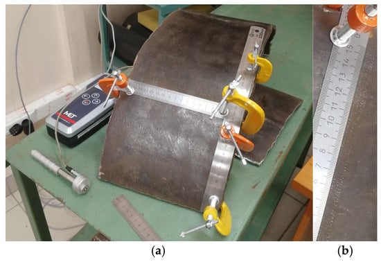
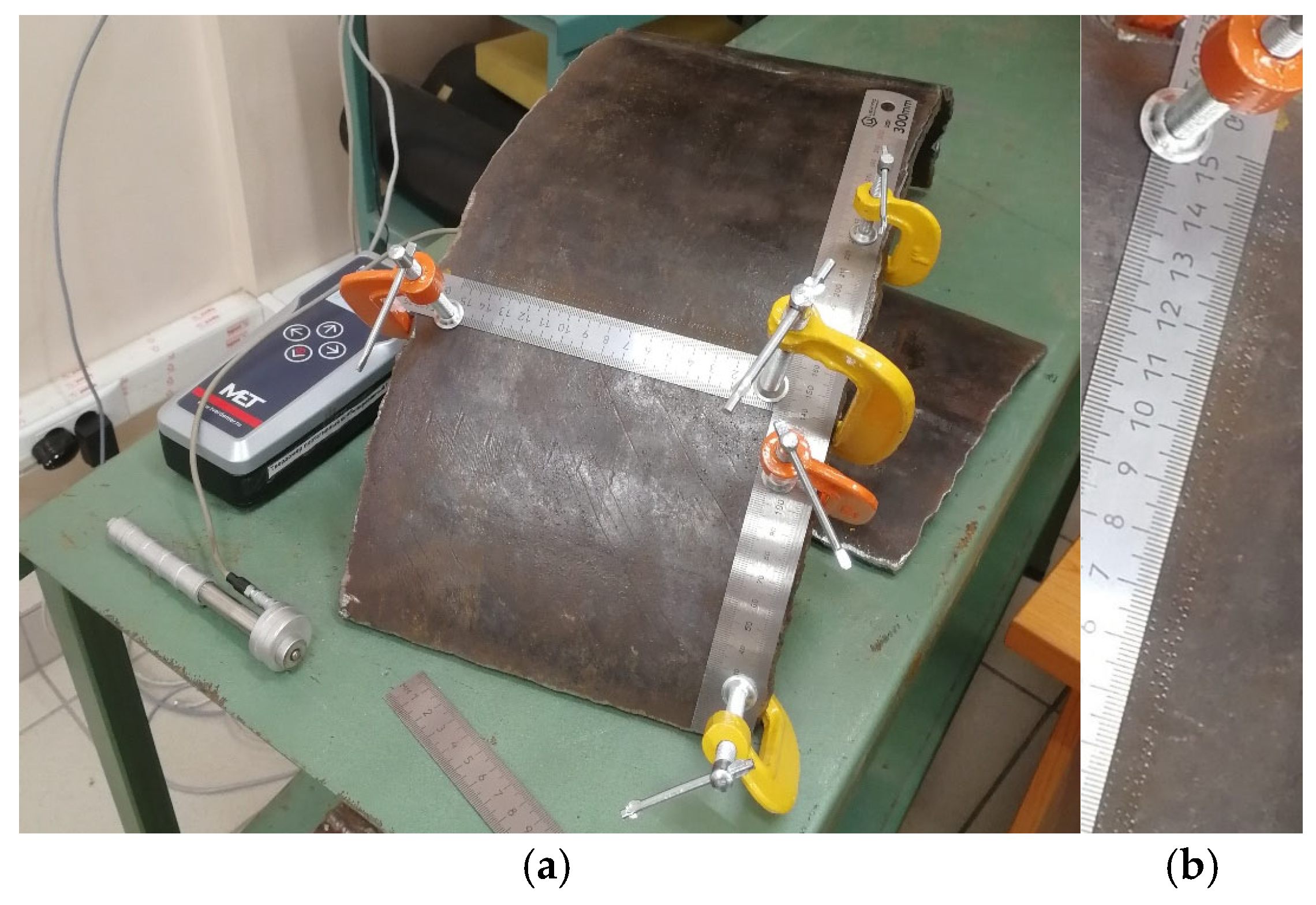
An image showing a general view of the test bench for an experiment to measure the hardness distribution over the test sample (TS) surface is given in Figure 1a and an enlarged image of the surface view being tested is shown in Figure 1b.
Figure 1.
Test bench for the experiment to measure the hardness distribution over the sample surface: (a) general view; (b) view of surface being tested.
2.2. Methods and Devices
Modern methods of hardness measurement and devices implementing them are known [49] to be highly accurate. Methods for measuring hardness are classified [49,50] by the method (Brinell, Vickers, Rockwell, Shore), by the time of the indenter effect on the CO, by the material and shape of the indenter, by the physical principle used, and by the level and the effect scale of the indenter on the CO. The effect scale determines the size of the object area affected by the indenter. Macro, micro, and nano levels are highlighted.
2.2.1. Methods for Measuring Hardness
Static and dynamic methods for measuring hardness are highlighted by the time and nature of the indenter effect on the CO. Static methods allow for an assessment of the hardness of steels with high accuracy, but it is difficult to apply them directly to pipeline transport facilities.
Dynamic and ultrasonic methods can be noted among the hardness measurement methods that can be applied in the field [51,52,53]. These methods are distinguished primarily by their high productivity and sufficient accuracy.
- Dynamic method for measuring hardness
It was noted in [54] that in dynamic methods of hardness measurement, the change in the kinetic energy of the indenter is estimated before and after interaction with the test material, and the results of this assessment determine the hardness of the material upon impact. The methods of Shore and Leeb in their various modifications continue to be the most relevant [54] among the dynamic methods of hardness measurement. The Leeb method is described in detail in [55,56]. The Leeb hardness value in its classical form is calculated by multiplying by 1000 the ratio of the striker’s rebound velocity to the impact velocity.
Currently, dynamic hardness meters use the Leeb approach, associated with measuring the indenter’s fall and rebound velocities and further estimating the hardness value in the selected scale using the resulting velocity ratio. A correct hardness assessment is possible in the case of bijection between the selected hardness scale and the range of changes in the velocity ratio or the Leeb scale [57]. Of course, the available data libraries for measuring hardness for the scales of interest and materials of interest to the researcher should completely cover the possible range of changes in the velocity ratios described above.
- Ultrasonic method for measuring hardness
The ultrasonic method for measuring hardness is based on the physical effect of the oscillatory system interaction with an elastic element connected to the indenter and a generator setting oscillations of a certain frequency with the surface of the CO [57]. This effect is called the ultrasonic contact impedance and manifests itself in a change in the oscillation frequency when the indenter is implemented into the surface of the CO. The system consists of the rod with the indenter in the free state that oscillates at a given frequency. The frequency is set by a piezoelectric generator. The oscillation receiver is connected to the oscillating system. The application of a load to the indenter results in its penetration into the object surface and a change in the oscillation frequency. The quantitative characteristic of the displacement of the oscillation frequency from the initial value is uniquely related to the hardness value.
2.2.2. Portable Devices for Measuring Hardness
MET-UDA (Centre MET LLC, Moscow, Russia) with ultrasonic and dynamic probes was chosen as a device designed for assessing the Brinell hardness [58].
The main technical and metrological characteristics of the MET-UDA hardness tester are given in Table 1 and Table 2.
Table 1.
Main technical characteristics of the MET-UDA hardness tester [58].
Table 2.
Metrological characteristics of the MET-UDA hardness tester [58].
3. Theory: Informative Hardness Measurement Parameters
The assessment of hardness H at a particular point of the tested product is a random variable. A random variable is completely determined if its distribution function FH(x) or its distribution density fH(x) are known. The distribution density has the greatest application in practice due to its graphical visualization. The entire set of numerical characteristics of RV is divided into position measures and scattering measures. Apart from the mean value, mode, and median, the parameters of functions describing RV distribution densities refer to the position measures; RV scattering measures include dispersion, SD and skewness, and kurtosis coefficients. Two groups of information parameters of the hardness measurement process will be highlighted below. The first group is represented by the hardness distribution density and the second one is represented by the numerical characteristics of the RV under consideration.
3.1. Hardness Distribution Densities
A number of distributions belonging to the class of two-parameter distributions are noted in the introduction as to be used for describing the hardness distribution density considered as RV. The following distributions are distinguished among this class [35,36,37]: normal; lognormal; Weibull; Gumbel. Based on the fact that the RV hardness H can only take positive values, it is more correct to consider the truncated normal distribution instead of the normal one. However, the average value of the Brinell hardness of pipe steels is large enough, and the level of the corresponding SD is not so significant to permit the probability of occurrence of hardness values close to zero in the sample, thus making it possible to ignore the remark noted above.
The formulas for the distributions noted above and graphs of the theoretical f(H) and sample fE(H) distribution densities are given in Table 3.
Table 3.
Distributions used in the process of measuring the hardness of steels.
The formulas for assessing sample distribution densities fE(H) have the form of
where H is a sample of hardness values; .
The results of calculations of distribution densities using the formulas from Table 3 are marked on the graphs by continuous curves and the sample distribution densities are shown in the bar graph. The analyzed distribution densities are unimodal; therefore, for the convenience of comparing f(H) and fE(H), it is recommended to choose an odd number of intervals in histograms, and the number of intervals in the histogram and, accordingly, the sample sizes N must be very significant.
3.2. Numerical Characteristics of the Hardness Assessment
The hardness assessment H, like any other RV, is known to be characterized by position measures and scattering measures. The expressions for calculating the theoretical and sample measures of position and scattering of the hardness assessment H are summarized in Table 4. In addition to the classical interpretation, the set of measures of position and dispersion is supplemented by the corresponding distribution parameters from Table 3.
Table 4.
Position and scattering measures of the hardness assessment H.
With regard to Table 3 and Table 4, to measure hardness repeatedly at the same point should be noted to be impossible since each single act of measuring hardness results in a change in the material structure at the marked point and its surroundings. Hence, the necessity to assess the hardness parameters by local areas follows.
3.3. Selection of Informative Parameters for the Hardness Measurement Process
A set of parameters characterizing hardness as a random variable is given in Table 3 and Table 4. The question emerges of choosing one or another characteristic of the considered RV as an informative parameter. Naturally, the traditional informative parameter for assessing the hardness of steel is its selective mean value . As is noted above, this parameter alone is not sufficient to assess the quality of new steel products, especially those subjected to technological effects to achieve the levels of hardness, strength, etc., specified by the consumer. The noted insufficiency manifests itself even more explicitly in case of the necessity to monitor the dynamics of changes in the technical condition of metal products having been exposed to various negative environmental factors for a long period of operation. These effects result not only in the bias of the average hardness assessments but also to an expansion of the range of changes in hardness assessments. The mean value assessment of the hardness of steel products under their service is supplemented by the measurement of SD [50,52].
It is obvious that the determination of any sample hardness parameters from Table 4 is not computationally difficult. It was noted above that an increase in the number of informative parameters in a number of cases leads to an increase in the likelihood of timely detection of negative trends in changes in the technical condition of operated metal products, for example, steel pipes. However, the sample distribution density with a large sample size N, a sufficient number of intervals in the histogram, and a significant number of points falling into each meaningful interval is close to the theoretical one and, therefore, has the maximum informative ability. All numerical characteristics of hardness assessments can be determined from the sample density of hardness distribution under the above conditions if it is necessary.
4. Experimental Assessment of Hardness Parameters of Pipe Steels
4.1. Conditions for Measuring Hardness
Information on the tested materials and samples is given in Section 2.1. Samples were cut from pipes having been in operation and Brinell hardness standards in the range from 100 HB to 200 HB were examined as TS.
The test surfaces of the pipe specimens were prepared for testing according to the MET-UDA instrument manual, meaning they were cleaned and polished. For the third and fourth specimens, a special solid plate with a rigid fixture was prepared, as the pipes were 7 mm thick, which is clearly insufficient for Brinell hardness testing with the MET-UDA dynamic hardness tester. The treated surfaces looked sufficiently smooth.
Two series of measurements were carried out. The measurements were carried out in the first series in order to compare two RVs: Brinell hardness assessments of the MET-UDA hardness tester with an impact action probe and an ultrasonic probe. The final result of analyzing the data from the first series is the selection of a probe for measuring hardness. The second series is intended to assess informative measurement parameters with the selected probe.
Brinell hardness measurements were carried out in strict accordance with the requirements of regulatory and technical documentation with periodic hardness measurements according to the above-mentioned Brinell hardness standards with the necessary correction of the corresponding scale.
A comparison of static and dynamic hardness assessments according to Brinell was not carried out, since at the present time, such a comparison, with rare exceptions, is not mandatory, since each of the groups of methods has its own areas of application and, in addition, as noted in [12], “However, currently (2025) there is neither a standardized definition, testing methodology nor technical specification for the machines used in hardness testing.”
The analysis of the first series of experiments results in the establishment of a large spread in ultrasonic probe readings; therefore, the work with the ultrasonic probe was stopped after collecting several hundred points of data on the first sample, and further measurements were carried out by means of a hardness tester with an impact action probe.
The surfaces prepared for testing were rectangular with dimensions A × B, mm, A > B. Hardness measurements done in the second series of experiments were carried out at the intersection points of the lines of two groups. The lines of the first group are perpendicular to the lines of the second group. This approach is caused by the necessity to generate appropriate digital images, which are matrices of dimension N × M, where N is the number of rows and M is the number of columns. The elements of the matrix H represent the distribution of Brinell hardness over the intersection points of the group lines described above. The total number of points in the images N × M generated for each tested sample exceeded 1000. The measurements were carried out along parallel lines with a probe displacement step along the line of 2 mm. The distance between parallel lines is 2 mm. The diameter of the indenter indentation mark ranged from 0.6 mm to 0.8 mm. This means the specified distance between the centers of the indentations exceeds the indentation diameter by 2.5 to 3.3 times. According to regulatory and technical documentation, a distance of 2 mm between the centers of two adjacent indentations is permitted when using the Met-UDA dynamic hardness tester.
4.2. Digital Images of Hardness
The Cartesian coordinate system XOY with the center in the upper left corner of the tested TS fragment is introduced for convenience. Point O coincides with the center of the first indentation mark. The matrix H representing the distribution of hardness assessments Hi j at points with coordinates xi, yj is received at the input of the algorithm for generating grayscale images of hardness.
where hx, hy are steps of x and y, respectively. For experimental conditions, hx = hy = 2 mm.
The expression for converting a digital image of hardness H into a grayscale image IH is
where floor (arg) is the integer part of arg; Imin, Imax are minimum and maximum gray level values, Imin ≥ 0, Imin < Imax ≤ 255.
In transformation (3), higher hardness assessments correspond to lighter areas of the image. Values Imin and Imax are selected from the conditions of visualization convenience.
When visually comparing the hardness images for several samples in Formula (3), the minimum and maximum hardness values for the entire set of samples are selected as the minimum and maximum hardness values.
Grayscale images of the hardness of four TSs of pipe steel for illustration purposes are given in Figure 2. Receiving more elements in the image without mechanization and automation is associated with certain difficulties of a subjective nature.
Figure 2.
Grayscale images of hardness.
In Figure 2, the excess of the average hardness level by three SD is marked in red, and the underestimation of the average hardness level by three SD is marked in blue. The analysis of the obtained grayscale images of hardness with color inclusions demonstrates the sections with reduced and increased hardness levels being present in all TS. An increase in the hardness of the metal during the operation of pipes leads to an increased likelihood of crack formation [63]. In turn, the presence of multiple microdefects leads to a decrease in the strength of the metal with a corresponding decrease in its hardness [63].
To make perception easy and selection of the tested surface fragments with increased and reduced hardness levels quick, color highlighting of the corresponding areas is resorted to. Levels of excess (understatement) are determined based on the analysis of standards and metrological characteristics of hardness meters.
4.3. Assessment of Random Variables Belonging to Distribution Classes
To test hypotheses about the analyzed RV (Brinell hardness) belonging to a certain distribution, it is necessary to calculate its parameters and check the proximity of the theoretical and sample distribution densities according to the corresponding criterion, for example, the Pearson’s chi-squared test (χ2) [64], or through using more modern and popular methods [65], such as the Kolmogorov–Smirnov, Cramer–von Mises, and Anderson–Darling goodness-of-fit tests.
There is a problem relating to the choice of criteria of consent. It is noted in [65] that in the minds of many researchers, a strong opinion has formed about criteria of the type χ2 as poor goodness-of-fit criteria. The authors of [65,66] do not agree with this opinion and emphasize that in the case of testing simple hypotheses and meeting a number of conditions, the fit criterion χ2 is preferable to the nonparametric fit tests of Kolmogorov, Cramer–Mises–Smirnov, and Anderson–Darling. Let us agree with the arguments of the authors of [65,66] and stop in our studies on the goodness-of-fit criterion χ2.
Table 5 summarizes the assessments of the distribution parameters from Table 4 for TS, digital images of hardness for which are given in Figure 2. The sample size for the first TS is N1 = 1037, the second one being N2 = 1136, and the third and fourth ones being N3 = N4 = 1020. Confidence intervals are indicated for the confidence probability Pγ = 95%. Confidence intervals for the main parameters were calculated using formulas from [67,68,69].
Table 5.
Experimental assessments of hardness parameters.
The analysis of the data presented in Table 5 results in the conclusion of a significant difference among the test samples in some hardness parameters. For example, samples 3 and 4 are similar in all position measures (mean, median, mode, μL, λW, λG) and differ significantly in all scattering measures (standard deviation, skewness, and kurtosis coefficients, kW and kG). This can be explained by the difference in operating conditions for the outer and inner surfaces of the pipes. For samples 1 and 2, the only thing that can be concluded is that they were cut from pipeline sections that operated under different operating conditions.
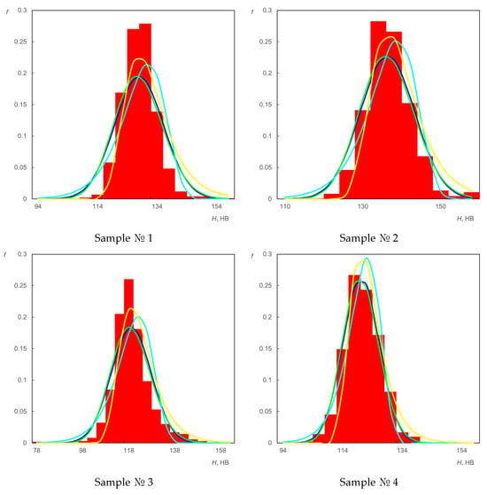
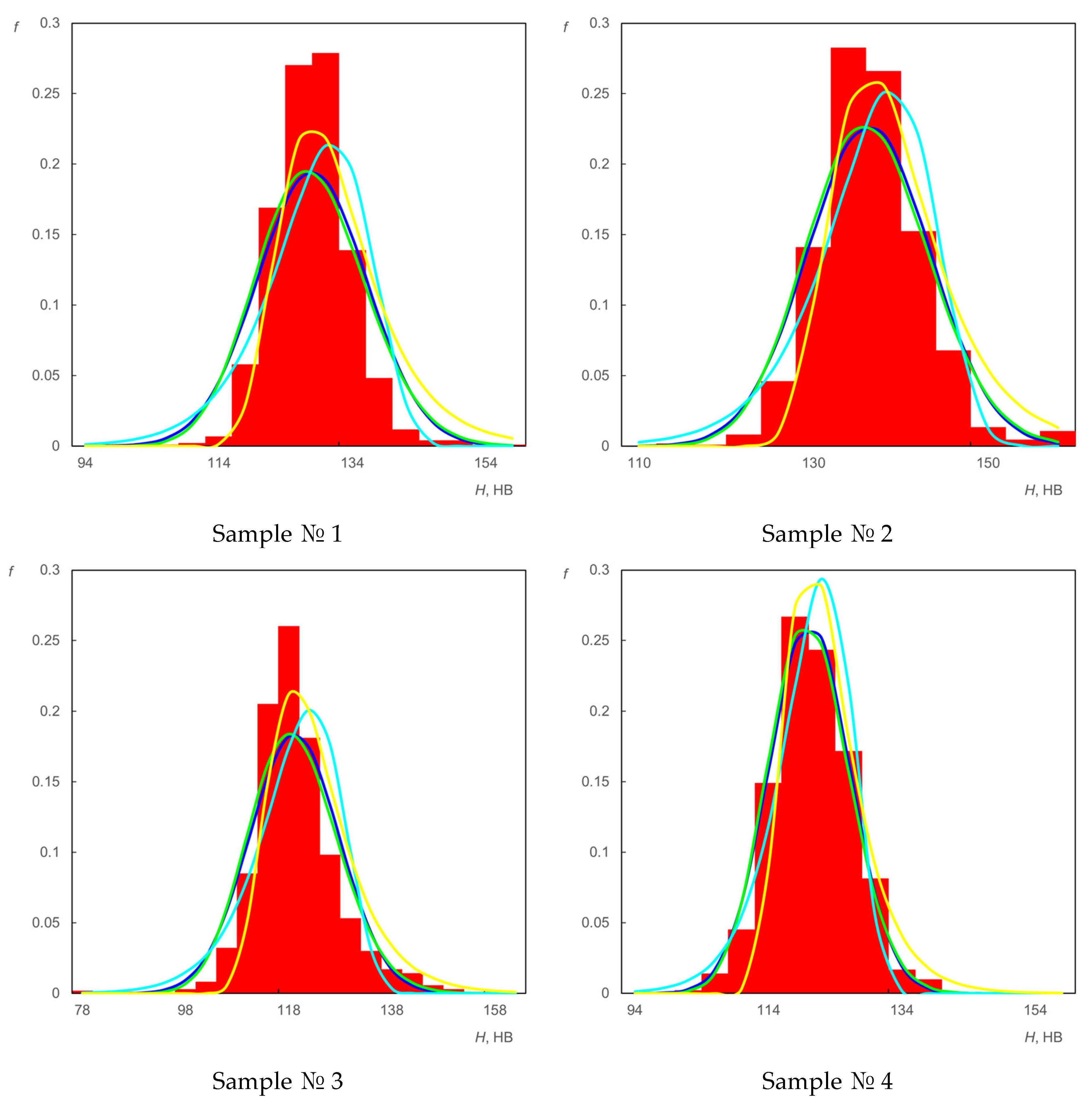
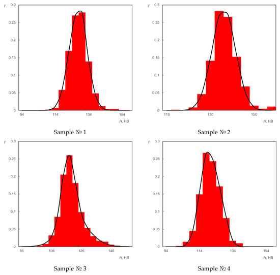
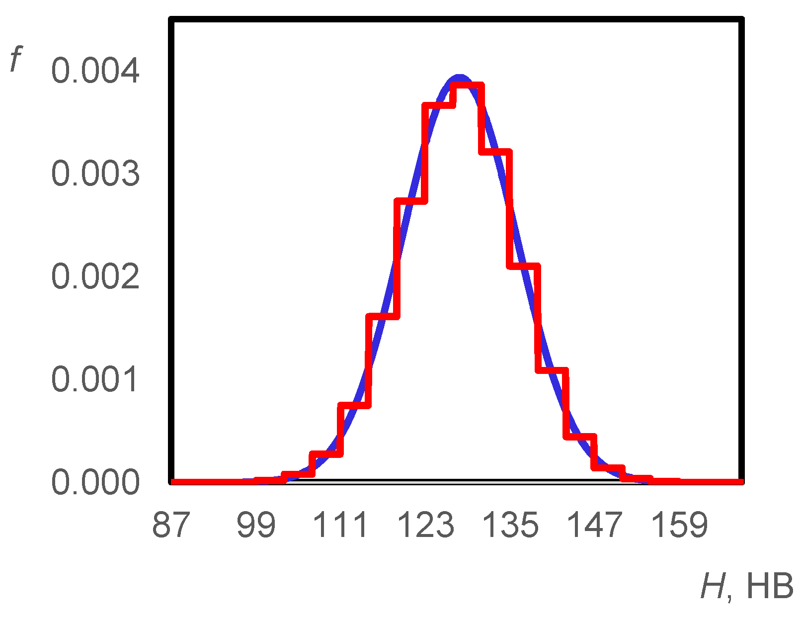
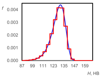
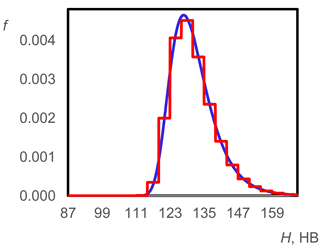
Figure 3 shows the assessment results of the sample and theoretical hardness distribution densities for hH = 4. A large number of formulas are known that allow one to choose the number of intervals n in histograms; most of them are mentioned in [65]. For a sample size N > 1000, it is recommended to choose n in the range of 12 to 16. We chose n = 14. The hypothetical densities of the normal distribution, the lognormal distribution, and the Weibull and Gumbel distributions were calculated for average values of parameters from Table 5.
Figure 3.
Assessments of sample and hypothetical densities of hardness distribution: ▌—sample distribution density;▬—normal distribution density; ▬—lognormal distribution density; ▬—Weibull distribution density; ▬—Gumbel distribution density.
The analysis of the data presented in Table 5 and Figure 3 results in the conclusion about a noticeable skewness and the leptokurtic nature of the experimental hardness distribution densities that makes it incorrect to use the normal and lognormal distributions to describe the investigated RV, at least for the steel samples under consideration in their specific technical condition.
The corresponding parameters of the chi-squared test (χ2) were calculated for more reliable confirmation of this conclusion and proof or refutation of the possibility of using the analyzed distributions to describe the studied RV. Table 6 shows the experimental and theoretical values and for both reliability coefficient β = 0.05 and the corresponding number of degrees of freedom k.
Table 6.
Experimental and theoretical assessments and for β = 0.05.
From a comparison of theoretical and experimental data presented in Table 6, it follows that with a confidence probability of 95%, it can be concluded that the experimental hardness distributions for pipe steel samples 1, 2, and 3 do not belong to the classes of normal distributions, lognormal distributions, Weibull distributions, or Gumbel distributions. Only for sample number 4 were the hypotheses about the normal and lognormal nature of the analyzed random variable confirmed.
Moreover, this confirmation is rather conditional, since the experimental values of are very close to the theoretical values of . Therefore, the final decision on whether the analyzed random variable belongs to the normal or lognormal distribution classes can be made based on the results of testing other goodness-of-fit tests, such as the Kolmogorov–Smirnov or Cramer–von Mises tests.
5. Discussion and Hypotheses
Micro- and macrostructural changes in the inner and outer surfaces of pipes are one of the most probable reasons for the asymmetric and leptokurtic nature of the hardness distribution densities of pipe steel samples that have been in long-term service. The noted changes result in either an increase or a reduction in the level of hardness of the steel surface layer. Moreover, this process is random; therefore, local areas with varying degrees of hardness change may be present on the surface. Steels have a micrograin structure, the elements of which (ferrite, perlite, martensite, bainite, etc.) differ in hardness [43,70]. The change in the relative content of these structural elements and their geometric and strength characteristics being in long-term operation leads to a change in hardness parameters [71].
Describing the probability density function of the hardness (microhardness) of materials, considered as a random variable, as a bimodal or multimodal function is justified in a number of cases [72,73,74]:
- It is justified when in the presence of two phases that differ significantly in hardness. For studying the technical condition of the surface of test steel objects, the change in the ratio of the phases during long-term operation is of particular interest. Most likely, the technical condition of the steel objects during operation in this case depends on the current ratio of the phases.
- A second reason for the appearance of bimodal distributions may be the presence of layer-by-layer heterogeneity, since in multilayer materials or materials with surface hardening, if the indenter depth reaches different layers, the hardness of the outer layer or the hardness of the underlying layer is predominantly assessed.
- A classic reason for the appearance of bimodal distributions is associated with the statistical heterogeneity of the structure of the alloy’s surface layer by grains; that is, the presence of zones with different grain sizes, especially during thermal or mechanical treatment, can give different hardness values.
5.1. Hypothesis on the Possibility of Describing the Hardness Distribution Density Using a Weighted Sum of Two Normal Distributions
Based on the foregoing, an assumption was made about the possible description of the distribution density of the analyzed RV by the bimodal function fB(H), for example, by the weighted sum of two normal distributions.
The function fB(H) (4) depends on five parameters—α, m1, σ1, m2, σ2—which can be found using the method of least squares.
5.2. Results of Estimation of Parameters of Bimodal Normal Functions for Test Samples
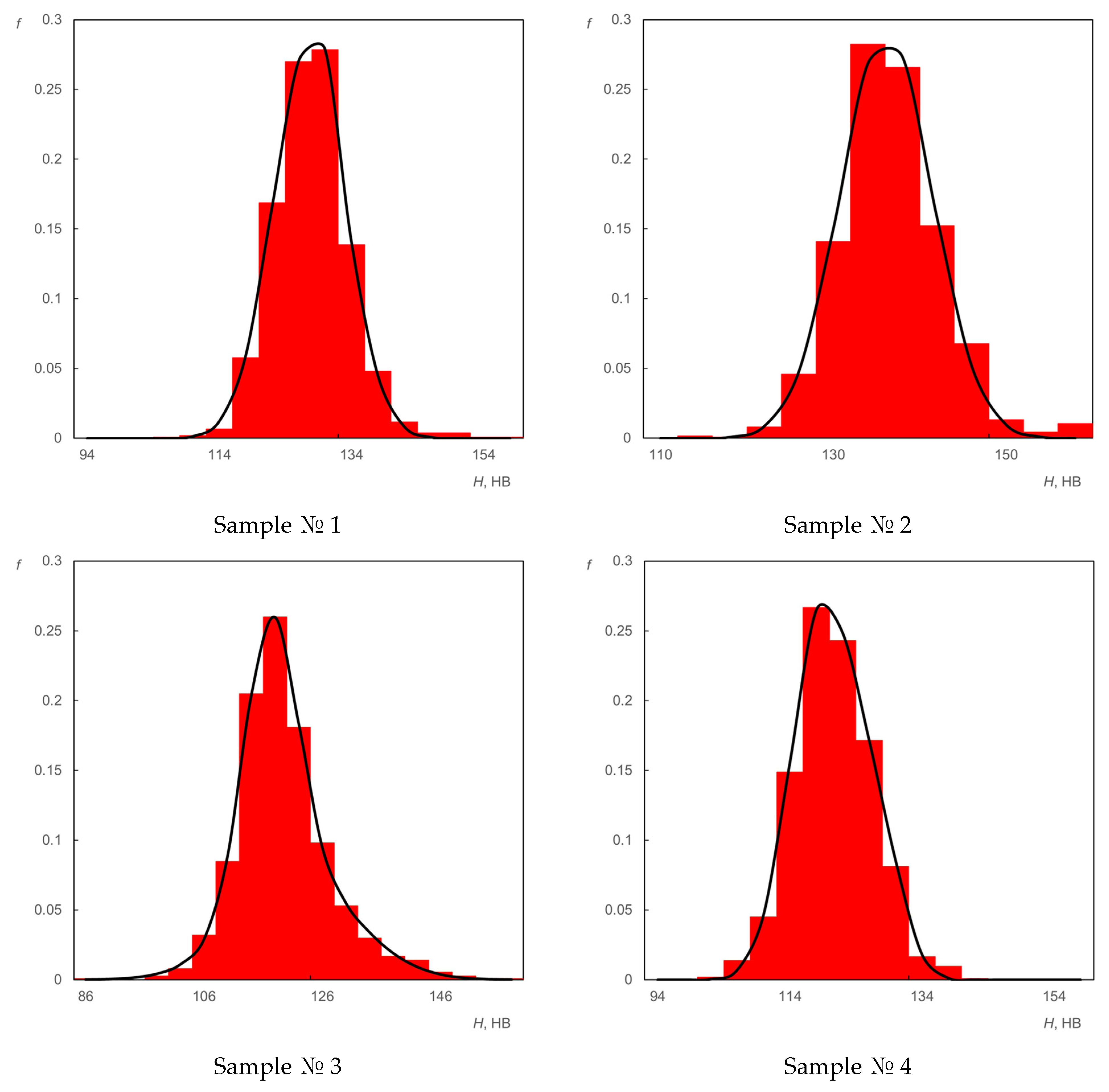
The results of calculating the parameters α, m1, σ1, m2, and σ2 using Formulas (4) and (5) are given in Table 7 to represent the Brinell hardness as a mixture of two random variables distributed according to Gauss. For the parameters m1, σ1, m2, and σ2, confidence intervals for a confidence level of 95% are indicated. Table 7 also shows experimental and theoretical assessments and for β = 0.05. The corresponding illustrative graphs of sample and hypothetical hardness distribution densities are shown in Figure 4.
Table 7.
Function parameters (4) with experimental and theoretical assessments and for β = 0.05.
Figure 4.
Assessments of sample and hypothetical densities of hardness distribution: ▌—sample distribution density; ──—mixture of normal distributions.
5.3. Testing Hypotheses About Steel Hardness Belonging to the Analyzed Classes of Distributions Using the Kolmogorov–Smirnov and Cramer–von Mises Criteria
In addition to the χ2 goodness-of-fit criterion, there are other criteria for testing hypotheses about the membership of the analyzed random variables—in our case, the Brinell hardness of steel—in the analyzed distributions classes. Such criteria include, for example, the Kolmogorov–Smirnov and Cramer–von Mises criteria.
Table 8 presents the results of experimental estimates of the SK parameters for the upper percentage point β = 0.05 of the Kolmogorov K(S) distribution when testing the simple hypothesis that the random variable under study belongs to one of the analyzed distribution classes. Table 8 also presents the results of experimental estimates of the Sω parameters for the upper percentage point β = 0.05 of the Cramer–von Mises ω2 statistic a1(S) when testing the simple hypothesis that the random variable under study belongs to one of the analyzed distribution classes.
Table 8.
Experimental and theoretical assessments SK and K(S) (Kolmogorov–Smirnov criterion) and Sω and a1(S) (Cramér–von Mises criterion) for β = 0.05.
If SK < K(S) for the Kolmogorov–Smirnov criterion or Sω < a1(S) for the Cramér–von Mises criterion, then the hypothesis that the random variable under analysis belongs to the analyzed class of distributions is confirmed; otherwise, the corresponding hypothesis is rejected.
Based on the analysis of the data presented in Table 8, the Kolmogorov–Smirnov criterion and the Cramér–von Mises criterion reject the hypotheses that the random variable under study belongs to the normal and lognormal distributions classes, as well as to the Weibull and Gumbel distribution classes.
A comparison of the theoretical and experimental values of χ2, the results from Table 8, and the analysis of the graphs in Figure 4 allow us to conclude that it is justified to represent the random variable under analysis (the hardness of steels in long-term use) as a mixture of two random normally distributed variables.
5.4. Future Research Directions
We list two main large-scale areas for future research.
- To determine the causes of changes in the position and hardness dispersion parameters of specimens, it is necessary to obtain estimates of these parameters at a certain initial time, and then regularly monitor changes in the analyzed parameters while simultaneously recording operating conditions and conducting microstructural analysis. An analysis of the collected information will allow us to hypothesize the causes of changes in the distribution function of the analyzed random variable and quantitatively link the characteristics of the hardness distributions to the degree of wear (degradation), thereby estimating the remaining service life of the tested pipeline.
- Obtaining digital images (surface hardness distribution maps) of the test objects is not an end in itself. The goal is to quickly detect negative changes in the objects by analyzing these images, as well as correctly interpret changes in the condition of the test object and conduct a corresponding, adequate risk assessment. This is especially important when using artificial intelligence methods to process digital images of mechanical parameters (maps), such as hardness, strength, etc. The results of some of the first practical applications of hardness distribution maps on the surface of particularly critical objects, in combination with other non-destructive testing methods, are presented in [75,76].
6. Conclusions
The features of measuring pipe steel hardness with dynamic and ultrasonic hardness meters are considered. A number of experiments were carried out on the formation of statistical samples of Brinell hardness values of a large volume of steel samples that were in long-term operation in harsh meteorological and functional conditions.
From the analysis of the experimental results, the following conclusions were obtained:
- We have shown the limited applicability of normal and lognormal distributions and Weibull and Gumbel distributions for describing the distribution density of hardness estimates for steels that have been in long-term operation in severe meteorological and functional conditions.
- We have described how the nature of the distributions of hardness estimates of the analyzed steel samples are applicable, which are weighted sums of two normal distributions.
- For non-destructive testing of the current technical condition of metal products that are in long-term operation under difficult conditions, and the dynamics of its change, it is effective to analyze digital images, which represent the distribution of hardness over the surface of the tested product.
- We have shown that the necessity of developing multi-channel mechanized or automated scanning hardness meters for the purpose of regular non-destructive assessment of the technical condition of main pipelines is substantiated.
It should be noted that the approaches proposed in this article can be used in cases of hardness assessment using macro- and micro-indentation or other physical methods for assessing the hardness of surface layers of products made of metals, alloys, and inorganic and organic solid materials, especially in the case of their operation in difficult conditions, which lead to the accelerated degradation of the analyzed objects.
Author Contributions
Conceptualization, S.O. and N.G.; methodology, S.O.; software, S.O.; validation, S.O., N.G., and O.B.; formal analysis, S.O.; investigation, N.G.; resources, N.G. and O.B.; data curation, S.O.; writing—original draft preparation, S.O.; writing—review and editing, N.G. and O.B.; visualization, O.B.; supervision, S.O.; project administration, O.B. All authors have read and agreed to the published version of the manuscript.
Funding
This research received no external funding.
Institutional Review Board Statement
Not applicable.
Informed Consent Statement
Not applicable.
Data Availability Statement
The original contributions presented in this study are included in the article. Further inquiries can be directed to the corresponding author.
Conflicts of Interest
Author Sergey Osipov was employed by the company Diagnostika-M LLC. The remaining authors declare that the research was conducted in the absence of any commercial or financial relationships that could be construed as a potential conflict of interest.
Abbreviations
The following abbreviations are used in this manuscript:
| CO | Control objects |
| SD | Standard deviation |
| RV | Random variable |
| TS | Test sample |
References
- Kowalczyk, M.; Andruszko, J.; Stefanek, P.; Mazur, R. Failure and Degradation Mechanisms of Steel Pipelines: Analysis and Development of Effective Preventive Strategies. Materials 2025, 18, 134. [Google Scholar] [CrossRef] [Scilit] [PubMed]
- Moradi, R.; Groth, K.M. Hydrogen storage and delivery: Review of the state of the art technologies and risk and reliability analysis. Int. J. Hydrogen Energy 2019, 44, 12254–12269. [Google Scholar] [CrossRef] [Scilit]
- Ijaola, A.O.; Farayibi, P.K.; Asmatulu, E. Superhydrophobic coatings for steel pipeline protection in oil and gas industries: A comprehensive review. J. Nat. Gas Sci. Eng. 2020, 83, 103544. [Google Scholar] [CrossRef] [Scilit]
- Qin, G.; Cheng, Y.F. A review on defect assessment of pipelines: Principles, numerical solutions, and applications. Int. J. Press. Vessel. Pip. 2021, 191, 104329. [Google Scholar] [CrossRef] [Scilit]
- Das, A.K. The present and the future of line pipe steels for petroleum industry. Mater. Manuf. Process. 2010, 25, 14–19. [Google Scholar] [CrossRef] [Scilit]
- Bassindale, C.; Wang, X.; Tyson, W.R.; Xu, S. Fast ductile fracture: Effect of inertia on propagation resistance and CTOA in pipe steels. Int. J. Press. Vessel. Pip. 2020, 187, 104163. [Google Scholar] [CrossRef] [Scilit]
- Borodin, V.I.; Lun-Fu, A.V.; Kudiiarov, V.N.; Lider, A.M.; Sakvin, I.S.; Bubenchikov, M.A.; Kaparulin, D.S.; Ovchinnikov, V.A. Application of the Electrochemical Permeation Method for Hydrogen Diffusion Coefficient Determination in Pipeline Steel 10G2. Coatings 2021, 11, 1260. [Google Scholar] [CrossRef] [Scilit]
- Qiurong, M. Microstructure design and properties of X100 gas line pipe. IOP Conf. Ser. Earth Environ. Sci. 2020, 585, 012025. [Google Scholar] [CrossRef] [Scilit]
- Timashev, S. Methodology of assessing individual reliability of unique structures. Russ. J. Constr. Sci. Technol. 2019, 5, 5–19. [Google Scholar] [CrossRef] [Scilit]
- Neganov, D.; Makhutov, N. Combined calculated, experimental and determinated and probable justifications for strength of trunk crude oil pipelines. In Probability, Combinatorics and Control; IntechOpen: London, UK, 2020; pp. 143–164. [Google Scholar] [CrossRef] [Scilit]
- Shtremel, M.A.; Arabei, A.B.; Glebov, A.G.; Abakumov, A.I.; Esiev, T.S.; Pyshmintsev, I.Y. Energy of the extended pipeline failure under pressure. Russ. Metall. 2021, 2021, 528–545. [Google Scholar] [CrossRef] [Scilit]
- Kuzu, C.; Germak, A.; Menelao, F.; Štibler, A.; Genta, G.; Loewit, M.; Borovský, J.; Maculotti, G.; Hiti, M.; Prato, A.; et al. Traceability for Indentation Measurements in Brinell-Vickers-Knoop Hardness. Meas. Sens. 2025, 38, 101453. [Google Scholar] [CrossRef] [Scilit]
- Yao, Z.; Tian, J.; Chen, X.; Wei, X.; Wang, J.; Xu, G. Investigation on microstructure and properties of low-carbon wear-resistant steels with addition of Cr and Ni. Steel Res. Int. 2020, 91, 1900677. [Google Scholar] [CrossRef] [Scilit]
- Mohammed, A.A.; Haris, S.M.; Al Azzawi, W. Estimation of the ultimate tensile strength and yield strength for the pure metals and alloys by using the acoustic wave properties. Sci. Rep. 2020, 10, 12676. [Google Scholar] [CrossRef] [Scilit]
- Jiao, J.; Lu, C.; Linton, V.; Barbaro, F. The effects of operational, testing, and material characterizations on the change in yield strength from plate to pipe. J. Press. Vessel Technol. 2021, 143, 041504. [Google Scholar] [CrossRef] [Scilit]
- Yang, H.; Chen, J.; Zhao, X.; Huda, N.; Gerlich, A.P. Effect of Filler Wire Composition on Weld Metal Microstructure and Mechanical Properties in X80 Steel Laser Welds. Materials 2024, 17, 5235. [Google Scholar] [CrossRef] [Scilit]
- Ding, S.; Tian, G.; Sutthaweekul, R. Non-destructive hardness prediction for 18CrNiMo7-6 steel based on feature selection and fusion of Magnetic Barkhausen Noise. NDT E Int. 2019, 107, 102138. [Google Scholar] [CrossRef] [Scilit]
- Zhao, X.; Liu, Z.; Gong, Y.; Huo, Z.; Chen, Z.; He, C.; Wu, B. Performance degradation detection of 12CrMoV steel by magneto-acoustic compound inspection method. NDT E Int. 2021, 124, 102525. [Google Scholar] [CrossRef] [Scilit]
- Fahse, D.N.; Levy, K.M.S.; Kim, J.Y.; Jacobs, L.J. Comparison of changes in nonclassical (α) and classical (β) acoustic nonlinear parameters due to thermal aging of 9Cr–1Mo ferritic martensitic steel. NDT E Int. 2020, 110, 102226. [Google Scholar] [CrossRef] [Scilit]
- Bjørheim, F.; Siriwardane, S.C.; Pavlou, D. A review of fatigue damage detection and measurement techniques. Int. J. Fatigue 2022, 154, 106556. [Google Scholar] [CrossRef] [Scilit]
- Kaimkuriya, A.; Sethuraman, B.; Gupta, M. Effect of Physical Parameters on Fatigue Life of Materials and Alloys: A Critical Review. Technologies 2024, 12, 100. [Google Scholar] [CrossRef] [Scilit]
- Bjørheim, F.; Pavlou, D.; Siriwardane, S.C. Hardness measurements as a technique for measuring accumulated fatigue damage. Int. J. Struct. Integr. 2022, 13, 699–716. [Google Scholar] [CrossRef] [Scilit]
- Silva, D.D.; Raimundo, R.A.; Alves, D.N.; Andrade, M.R.; Torquato, R.A.; Gomes, R.M.; Morales, M.A.; Oliveira, D.F. Evaluation of mechanical ductile damage in sheet metal based on low-field magnetic analysis. J. Magn. Magn. Mater. 2021, 539, 168403. [Google Scholar] [CrossRef] [Scilit]
- Khattak, M.A.; Zareen, N.; Mukhtar, A.; Kazi, S.; Jalil, A.; Ahmed, Z.; Jan, M.M. Root cause analysis (RCA) of fractured ASTM A53 carbon steel pipe at oil & gas company. Case Stud. Eng. Fail. Anal. 2016, 7, 1–8. [Google Scholar] [CrossRef] [Scilit]
- Ding, H.; Qi, D.T.; Qi, G.Q.; Wei, B.; Ding, N.; Li, H.B.; Wang, F.S.; Yan, Z.F.; Feng, Q.; Zhang, Z.F.; et al. Cracking analysis of a newly built gas transmission steel pipe. Eng. Fail. Anal. 2020, 118, 104868. [Google Scholar] [CrossRef] [Scilit]
- PN-EN ISO 6508-1:2007; Metallic Materials—Rockwell Hardness Test—Part 1: Test Method. Polish Committee for Standardization: Warsaw, Poland, 2007.
- PN-EN ISO 6508-2:2007; Metallic Materials—Vickers Hardness Test—Part 2: Verification and Calibration of Testing Machines. Polish Committee for Standardization: Warsaw, Poland, 2007.
- PN-EN ISO 6508-3:2007; Metallic Materials—Rockwell Hardness Test—Part 3: Calibration of Reference Blocks. Polish Committee for Standardization: Warsaw, Poland, 2007.
- Low, S.R. Rockwell Hardness Measurement of Metallic Materials. In NIST Recommended Practice Guide; Volume Special Publication 960-5; National Institute of Standards and Technology: Gaithersburg, MD, USA, 2001. [Google Scholar]
- Gargalis, L.; Karavias, L.; Graff, J.S.; Diplas, S.; Koumoulos, E.P.; Karaxi, E.K. A Comparative Investigation of Duplex and Super Duplex Stainless Steels Processed through Laser Powder Bed Fusion. Metals 2023, 13, 1897. [Google Scholar] [CrossRef] [Scilit]
- Koga, N.; Suzuki, S.; Jiang, H.; Watanabe, C.; Aoyagi, Y.; Kobayashi, M.; Miura, H. Characterization of heterogeneous–nano structure in austenitic stainless steel: Crystal orientations and hardness distribution. J. Mater. Sci. 2020, 55, 9299–9310. [Google Scholar] [CrossRef] [Scilit]
- Nykyforchyn, H.; Zvirko, O.; Dzioba, I.; Krechkovska, H.; Hredil, M.; Tsyrulnyk, O.; Student, O.; Lipiec, S.; Pala, R. Assessment of Operational Degradation of Pipeline Steels. Materials 2021, 14, 3247. [Google Scholar] [CrossRef] [Scilit] [PubMed]
- Zvirko, O.; Tsyrulnyk, O.; Nykyforchyn, H. Non-destructive evaluation of operated pipeline steel state taking into account degradation stage. Procedia Struct. Integr. 2020, 26, 219–224. [Google Scholar] [CrossRef] [Scilit]
- Beltrán-Zúñiga, M.A.; Rivas-López, D.I.; Dorantes-Rosales, H.J.; González-Zapatero, W.; Ferreira-Palma, C.; López-Hirata, V.M.; Hernández-Santiago, F. Fatigue life assessment of low carbon API 5L X52 pipeline steels retired from long-term service. Eng. Fail. Anal. 2023, 143, 106769. [Google Scholar] [CrossRef] [Scilit]
- Schneider, J.-M.; Bigerelle, M.; Iost, A. Statistical analysis of the Vickers hardness. Mater. Sci. Eng. A 1999, 262, 256–263. [Google Scholar] [CrossRef] [Scilit]
- Bogdanoff, T.; Tiryakioğlu, M.; Liljenfors, T.; Jarfors, A.E.W.; Seifeddine, S.; Ghassemali, E. On the Effectiveness of Rotary Degassing of Recycled Al-Si Alloy Melts: The Effect on Melt Quality and Energy Consumption for Melt Preparation. Sustainability 2023, 15, 5189. [Google Scholar] [CrossRef] [Scilit]
- Lebedev, A.A.; Makovetskii, I.V.; Muzyka, N.R.; Volchek, N.L.; Shvets, V.P. Assessment of damage level in materials by the scatter of elastic characteristics and static strength. Strength Mater. 2006, 38, 109–116. [Google Scholar] [CrossRef] [Scilit]
- Gasimov, G.R.; Rzayev, Y.R. Probabilistic-statistical investigation of the evolution processes of particle distributions in oil dispersed systems in the maple software environment. J. Umm Al-Qura Univ. Appl. Sci. 2026. [Google Scholar] [CrossRef] [Scilit]
- Lebedev, A.A.; Makovetskii, I.V.; Muzyka, N.R.; Shvets, V.P. A study of deformation and damage accumulation processes in 10GN2MFA steel under low-cycle loading. Strength Mater. 2008, 40, 163–167. [Google Scholar] [CrossRef] [Scilit]
- Poberezhny, L.; Stanetsky, A.; Grytsuliak, G.; Poberezhna, L.; Kosmii, M.; Hrytsanchuk, A. Corrosion-mechanical behavior of gas main steel in saline soils. Koroze Ochr. Mater. 2019, 63, 105–112. [Google Scholar] [CrossRef] [Scilit]
- Bailey, A.V.; Miri, M.J.; Press, R.J.; Santhanam, K.S.V.; Takacs, G.A. Introduction to Hydrogen Technology; John Wiley & Sons, Inc.: Rochester, NY, USA, 2018; 432p. [Google Scholar]
- Ura-Bińczyk, E.; Dobkowska, A.; Płocińska, M.; Płociński, T.; Adamczyk-Cieślak, B.; Mazurkiewicz, B.; Solarski, W.; Banaś, J.; Mizera, J. The influence of grain refinement on the corrosion rate of carbon steels in fracturing fluids used in shale gas production. Mater. Corros. 2017, 68, 1190–1199. [Google Scholar] [CrossRef] [Scilit]
- Kupriyanova, O.A. New Generation High-Strength Cold-Resistant Steels: History, Current Status and Development Prospects. Steel Transl. 2023, 53, 571–577. [Google Scholar] [CrossRef] [Scilit]
- Nastich, S.Y.; Kornilov, V.L.; Morozov, Y.D.; Denisov, S.V.; Molostov, M.A. New steels for pipelines of strength classes K54-K60 (X70): Production experience at OAO MMK. Steel Transl. 2009, 39, 431–436. [Google Scholar] [CrossRef] [Scilit]
- API. Specification for Line Pipe: API Specification 5L, 46th ed.; American Petroleum Institute: Washington, DC, USA, 2018. [Google Scholar]
- Kuberskii, S.V.; Sbitnev, S.A.; Velikotskii, R.E.; Dolzhkov, V.V. Influence of Phase Composition and Aging on Hydrogen Brittleness of High-Pressure Pipelines. Steel Transl. 2023, 53, 1181–1188. [Google Scholar] [CrossRef] [Scilit]
- Tovmasyan, M.A.; Samusev, S.V. Effect of the Nonuniform Distribution of the Mechanical Properties of Rolled Sheets on the Shape of a Round Billet after Forming in Making Large-Diameter Pipes. Russ. Metall. 2020, 2020, 589–596. [Google Scholar] [CrossRef] [Scilit]
- Panin, S.V.; Vlasov, I.V.; Maruschak, P.O.; Eremin, A.V.; Berto, F.; Syromyatnikova, A.S.; Vinogradov, A. Influence of long-term cold climate operation on structure, fatigue durability and impact toughness of 09Mn2Si pipe steel. Eng. Fail. Anal. 2019, 102, 87–101. [Google Scholar] [CrossRef] [Scilit]
- Broitman, E. Indentation hardness measurements at macro-, micro-, and nanoscale: A critical overview. Tribol. Lett. 2017, 65, 23. [Google Scholar] [CrossRef] [Scilit]
- Rebouças Filho, P.P.; da Silveira Cavalcante, T.; de Albuquerque, V.H.C.; Tavares, J.M.R. Brinell and Vickers hardness measurement using image processing and analysis techniques. J. Test. Eval. 2010, 38, 88–94. [Google Scholar] [CrossRef] [Scilit]
- Hampton, J.C.; Boitnott, G.N.; Louis, L. A New dynamic indentation tool for rapid mechanical properties profiling and mapping. Rock Mech. Rock Eng. 2022, 55, 2597–2613. [Google Scholar] [CrossRef] [Scilit]
- Fayustov, A.A.; Novokshonova, O.D. Innovative methods for rapid control of material hardness. IOP Conf. Ser. Mater. Sci. Eng. 2021, 1079, 052063. [Google Scholar] [CrossRef] [Scilit]
- Hsia, S.Y.; Chou, Y.T. Assessing the hardness of quenched medium steel using an ultrasonic nondestructive method. Adv. Mater. Sci. Eng. 2015, 2015, 684836. [Google Scholar] [CrossRef] [Scilit]
- Oreshko, E.I.; Utkin, D.A.; Yerasov, V.S.; Lyakhov, A.A. Methods of measuring the hardness of materials (review). Proc. VIAM. 2020, 85, 101–117. [Google Scholar] [CrossRef] [Scilit]
- Leeb, D. Dynamic hardness testing of metallic materials. NDT E Int. 1979, 12, 274–278. [Google Scholar] [CrossRef] [Scilit]
- Potapov, A.I.; Syasko, V.A.; Gogolinsky, K.V.; Nikonov, A.A. Ensuring the uniformity of hardness measurements by the dynamic method in the Russian Federation. Control. Diagn. 2016, 4, 44–49. [Google Scholar] [CrossRef] [Scilit]
- Gogolinskii, K.V.; Syasko, V.A.; Umanskii, A.S.; Nikazov, A.A.; Bobkova, T.I. Mechanical properties measurements with portable hardness testers: Advantages, limitations, prospects. J. Phys. Conf. Ser. 2019, 1384, 012012. [Google Scholar] [CrossRef] [Scilit]
- MET-UDA Hardness Tester. Available online: https://www.tverdomer.ru/products/portable-hardness-testers/ud/ (accessed on 25 March 2026).
- Montgomery, D.; Runger, G. Applied Statistics and Probability for Engineers; John Wiley & Sons: New York, NY, USA, 2018. [Google Scholar]
- Alam, M.; Farnham, C.; Emura, K. Best-Fit Probability Models for Maximum Monthly Rainfall in Bangladesh Using Gaussian Mixture Distributions. Geosciences 2018, 8, 138. [Google Scholar] [CrossRef] [Scilit]
- Garrido, A. Symmetry and Asymmetry Level Measures. Symmetry 2010, 2, 707–721. [Google Scholar] [CrossRef] [Scilit]
- Nadarajah, S.; Kotz, S. The beta Gumbel distribution. Math. Probl. Eng. 2004, 2004, 323–332. [Google Scholar] [CrossRef] [Scilit]
- Schipachev, A.; Aljadly, M.; Ganzulenko, O.; Chernikov, D.; Razzhivin, V.; Yusupov, R. Evaluating the Effectiveness of Magnetic-Pulse Treatment for Healing Continuity Defects in the Metal of Oil and Gas Pipelines. Metals 2023, 13, 1875. [Google Scholar] [CrossRef] [Scilit]
- Heinhold, I.; Gaede, K.W. Ingeniur Statistic; Springler: München, Germany; Wien, Austria, 1964; 352p. [Google Scholar]
- Lemeshko, B.Y.; Lemeshko, S.B.; Postovalov, S.N.; Chimitova, E.V. Statistical Data Analysis, Simulation and Study of Probability Regularities. Computer Approach: Monograph; NSTU-Publisher: Novosibirsk, Russia, 2011; 888p. [Google Scholar]
- Lemeshko, B.Y.; Lemeshko, S.B.; Postovalov, S.N. Comparative analysis of the power of goodness-of-fit tests for near competing hypotheses. I. The verification of simple hypotheses. J. Appl. Ind. Math. 2009, 3, 462–475. [Google Scholar] [CrossRef] [Scilit]
- Donner, A.; Zou, G.Y. Closed-form confidence intervals for functions of the normal mean and standard deviation. Stat. Methods Med. Res. 2012, 21, 347–359. [Google Scholar] [CrossRef] [Scilit] [PubMed]
- Gillard, J. Confidence Intervals. In A First Course in Statistical Inference; Springer Undergraduate Mathematics Series; Springer: Cham, Switzerland, 2020; pp. 45–61. [Google Scholar] [CrossRef] [Scilit]
- D’agostino, R.B.; Belanger, A.; D’Agostino, R.B., Jr. A suggestion for using powerful and informative tests of normality. Am. Stat. 1990, 44, 316–321. [Google Scholar] [CrossRef] [Scilit]
- Protopopov, E.; Dobrykh, S.; Trofimova, Y.; Malenko, P.; Valter, A.; Protopopov, A. Reflection of strengthening results in values of generalized degrees of metallicity and covalence is principle to new strategy of designing alloys. Sci. Rep. 2020, 10, 2050. [Google Scholar] [CrossRef] [Scilit] [PubMed]
- González-Arévalo, N.E.; Velázquez, J.C.; Díaz-Cruz, M.; Cervantes-Tobón, A.; Terán, G.; Hernández-Sanchez, E.; Capula-Colindres, S. Influence of aging steel on pipeline burst pressure prediction and its impact on failure probability estimation. Eng. Fail. Anal. 2021, 120, 104950. [Google Scholar] [CrossRef] [Scilit]
- Chakrabarti, D.; Strangwood, M.; Davis, C. Effect of Bimodal Grain Size Distribution on Scatter in Toughness. Metall. Mater. Trans. A 2009, 40, 780–795. [Google Scholar] [CrossRef] [Scilit]
- Gholamalipour, S.; Jamaati, R.; Hosseinipour, S.J. The effect of high-temperature intercritical annealing and rolling strain on the development of trimodal microstructure in low-carbon steel. J. Mater. Res. Technol. 2025, 34, 1529–1538. [Google Scholar] [CrossRef] [Scilit]
- Gocnik, M.; Hatzenbichler, L.; Meindlhumer, M.; Haslberger, P.; Galler, M.; Stark, A.; Olsson, C.-O.A.; Keckes, J.; Schnitzer, R. Influence of Tramp Elements on Phase Transformations, Microstructure and Hardness of a 0.3 wt.%C Low-Alloyed Steel. Metals 2025, 15, 1053. [Google Scholar] [CrossRef] [Scilit]
- Li, D.; Wang, H.; Shen, X.; Lin, S.; Feng, H.; Peng, Y.; Jiang, F.; Zhou, X. Quantitative Distribution Characterization and Correlation Study of Composition, Structure and Hardness of Rim Region in Railway Wheel. Materials 2022, 15, 4762. [Google Scholar] [CrossRef] [Scilit]
- Liu, Z.; Yang, L.; Zhang, G.; Zhao, L.; Shao, Q.; Huang, D.; Zhu, Y.; Wang, X.; Shen, Z.; Yang, H.; et al. Correlation of microstructure and hardness distribution of high-speed train wheels under original and service statuses. Eng. Fail. Anal. 2024, 158, 107994. [Google Scholar] [CrossRef] [Scilit]



Disclaimer/Publisher’s Note: The statements, opinions and data contained in all publications are solely those of the individual author(s) and contributor(s) and not of MDPI and/or the editor(s). MDPI and/or the editor(s) disclaim responsibility for any injury to people or property resulting from any ideas, methods, instructions or products referred to in the content. |
© 2026 by the authors. Licensee MDPI, Basel, Switzerland. This article is an open access article distributed under the terms and conditions of the Creative Commons Attribution (CC BY) license.