


Abstract
Early, non-invasive detection of the critical heat flux (CHF) is essential for the safe operation of nuclear, electronic-cooling and other high-heat-flux systems, yet conventional thermocouple-based monitoring is invasive, slow and point-wise. This paper presents an explainable deep-learning framework that classifies high-speed pool-boiling imagery into pre-CHF and post-CHF regimes and, in the same forward pass, regresses the energy-balance-derived equivalent vapour mass flux m″v. The proposed DL-Optimum model—a ResNet-50 backbone augmented with Squeeze-and-Excitation channel attention, label smoothing, cosine-annealed warm restarts and five-crop test-time augmentation—is benchmarked against six architectures on the open NED3 pool-boiling corpus of 3000 frames, and a stepwise ablation ladder (A0–A4) quantifies the cumulative contribution of each modification. DL-Optimum attains the highest performance (accuracy 0.9622, F1 0.9625, AUC-ROC 0.9772), reproduced under five-fold cross-validation (0.9622 ± 0.0058), confirmed on each of the five condition groups individually (0.939–0.983) and generalising to entirely unseen condition groups under leave-one-group-out cross-validation (0.8827 ± 0.0293). The regression head achieves an MAE of 0.041 kg·m−2·s−1 (R2 = 0.913) against the energy-balance ground truth. Grad-CAM attributions are consistent with physically relevant regions—nucleation-site activity and vapour-blanket morphology—Monte-Carlo Dropout yields calibrated confidence (predictive entropy 0.0674 ± 0.1024), and stress tests retain 0.902 accuracy from 10% of the training data and 0.938 at σ = 0.20 additive noise. An accuracy–efficiency analysis identifies DL-Optimum as accuracy-Pareto-optimal (26.30 M parameters; 332 FPS single-pass, ≈33 FPS under the full ten-pass test-time-augmentation protocol) and EfficientNet-B0 as efficiency-Pareto-optimal, and DL-Optimum achieves a 3.2 percentage-point higher in-distribution accuracy than the best published image-based CHF baseline (0.930) and a 1.2 percentage-point higher accuracy than the published acoustic baseline (0.950), though direct comparisons remain subject to cross-study differences in datasets and evaluation protocols.
1. Introduction
Boiling heat transfer is among the most efficient mechanisms for removing high heat fluxes and is therefore central to the thermal management of nuclear reactors, high-power electronics, aerospace propulsion and advanced manufacturing [1]. The usable range of nucleate boiling is bounded by the critical heat flux (CHF), beyond which a vapour film blankets the heated surface, the heat-transfer coefficient collapses and the wall temperature can rise catastrophically—the so-called boiling crisis [1,2]. Reliable and timely detection of the approach to CHF is consequently a prerequisite for the safety of nuclear water-cooled reactors, for two-phase direct-immersion cooling of high-power computing [3] and for cryogenic and aerospace propulsion systems.
In practice, CHF is monitored primarily with intrusive thermal sensors—embedded thermocouples or fibre-optic probes—whose finite thermal mass and conduction path limit temporal resolution, perturb the observed surface and provide only point-wise evidence of the two-phase morphology that governs the transition. High-speed optical visualisation, by contrast, captures the bubble nucleation, growth, coalescence and vapour-removal dynamics that physically determine CHF, making it an attractive basis for non-intrusive, full-field monitoring. Although machine learning is now established in fluid mechanics and heat transfer [4], translating it into a dependable, interpretable CHF monitor remains an open problem. A second gap concerns the vapour mass flux m″v leaving the heater, which governs the vapour-removal load on the condenser, the coolant-loop mass flow rate and the safety margin against dry-out, yet is normally derived post hoc from heat-flux measurements; a learning-based monitor that estimates both the regime label and the instantaneous m″v from the same image stream would close both gaps simultaneously.
The direct application of deep learning to boiling imagery for CHF detection was pioneered by Rassoulinejad-Mousavi et al. [5] and extended to supervised and unsupervised detection by Dunlap et al. [6]. In parallel, the community has released open multimodal boiling datasets synchronising optical, acoustic and thermal measurements [7,8,9], non-intrusive acoustic characterisations of the boiling state [10,11] and synchronous visual–infrared partitionings of boiling heat-transfer mechanisms [12]. Existing image-based CHF studies, however, evaluate only a narrow set of largely classical architectures, treat the network as a black box and report point accuracy without characterising model confidence, robustness or labelling requirements—properties essential before any learning-based monitor can be trusted in a safety-critical loop.
This work closes these gaps. We benchmark six established architectures— ResNet-50 [13], EfficientNet-B0/B4, ConvNeXt-Tiny [14], ViT-B/16 [15] and a from-scratch CNN—on the open NED3 pool-boiling image set [16], and propose DL-Optimum, a ResNet-50 backbone augmented with Squeeze-and-Excitation (SE) channel attention [17], label smoothing, cosine-annealed warm restarts [18] and five-crop test-time augmentation (TTA). All models are subjected to Grad-CAM interpretation [19], Monte-Carlo Dropout uncertainty analysis [20] and data-efficiency, noise-robustness, cross-validation and inference-speed stress tests. In response to the review, the validation protocol additionally comprises (i) a stepwise architectural ablation that isolates the contribution of each proposed modification (Section 3.7 and Section 4.3), (ii) a leave-one-group-out (LOGO) evaluation in which the model is trained on four condition groups and tested on the entirely unseen fifth group—four heater-surface types or the transient heating protocol (Section 3.7 and Section 4.4), (iii) interpretability statements calibrated to what Grad-CAM can and cannot establish (Section 4.5) and (iv) an explicit account of the validity, uncertainty and target-dependence of the energy-balance-derived regression ground truth (Section 2.3).
Relative to the closest published CHF-DL studies [5,6,10], the present study delivers, in a single framework, a seven-architecture benchmark with interpretability and validation analyses, per-surface invariance evidence, uncertainty characterisation and an accuracy–efficiency frontier. Following the review, the novelty framing is consolidated into three scientific pillars:
(P1) The DL-Optimum classification framework and its stepwise architectural ablation. A ResNet-50 backbone augmented withSqueeze-and-Excitation channel attention [17], label smoothing [21], cosine-annealed warm restarts [18] and ten-pass test-time augmentation, benchmarked against six established architectures (ResNet-50, EfficientNet-B0/B4, ConvNeXt-Tiny, ViT-B/16 and a from-scratch CNN) on the open NED3 corpus, with a controlled ablation ladder (Section 4.3) that quantifies the cumulative contribution of each modification and an accuracy–efficiency frontier that quantifies the deployment cost of each model.
(P2) Physics-consistent interpretability and uncertainty-aware, group-wise validation. Grad-CAM attributions that are consistent with physically relevant regions—distinguishing class-discriminative relevance (discrete nucleation clusters in pre-CHF vs. contiguous vapour columns in post-CHF) from a uniformly cold bulk-liquid background—paired with Monte-Carlo Dropout calibration (predictive entropy0.0674 ± 0.1024 and a reliability diagram), leave-one-group-out generalisation to unseen experimental condition groups, per-surface confusion matrices, and data-efficiency and noise-robustness stress tests. The scope and limits of the Grad-CAM evidence are stated explicitly, and the deployment language is calibrated to the in-distribution character of the uncertainty analysis.
(P3) Joint continuous regression of the vapour mass flow rate. A shared-backbone regression head that returns the regime label and the energy-balance-derived equivalent vapour mass flux m″v (MAE 0.041 kg·m−2·s−1, R2 = 0.913) in a single forward pass, with the validity conditions of the ground truth, its uncertainty and its shared physical dependence on the classification target stated explicitly (Section 2.3 and Section 5).
The remainder of this paper is organised as follows. Section 2 describes the facility, the NED3 corpus, the vapour-mass-flux ground truth and the boiling-curve-based labelling; Section 3 details the architectures, the training protocol and the interpretability, uncertainty and stress-test methodology, and introduces the LOGO and stepwise-ablation protocols (Section 3.7); Section 4 presents the results; Section 5 discusses deployment implications and limitations, including a quantified comparison against thermal-sensor response; and Section 6 concludes.
2. Experimental Dataset and Data Collection
2.1. Multimodal Pool-Boiling Facility and Instrumentation
We state explicitly that neither the facility shown in Figure 1 and Figure 2 nor the underlying experiments originate from the present authors: both the schematic and the photographs are reproduced from the open data paper of Pandey et al. [7].
Figure 1.
Schematic of the heating-element enclosure of the pool-boiling test facility with the synchronised optical, acoustic and thermal sensing channels [7].
Figure 2.
Pool-boiling test facility with the multimodal sensing instrumentation in place: high-speed camera, hydrophones submerged in the pool (a) and the MISTRAS R3a acoustic-emission sensor attached to the bottom of the chamber (b).
Figure 2 shows the physical facility with the multimodal instrumentation in place. The boiling chamber is a closed tank with a PEEK base housing the heating enclosure, a 1 cm × 1 cm copper-block heater surface powered by cartridge heaters, and a chiller–condenser cooling loop. Boiling is visualised by a Phantom VEO 710L high-speed camera (Vision Research, Inc., Wayne, NJ, USA) with LED backlighting. The thermocouple and hydrophone channels are routed to a National Instruments (NI) cDAQ-9178 chassis populated with an NI 9210 temperature module (for the four block thermocouples and two additional pool/vapour thermocouples), an NI 9230 sound-and-vibration module (for the hydrophone) and an NI 9239 voltage-input module (for the chamber pressure transducer) (National Instruments, Austin, TX, USA); the chassis is controlled by a LabVIEW application that exports the time-synchronised traces as LabVIEW measurement (.lvm) files (National Instruments, Austin, TX, USA). The hydrophone is a High Tech, Inc. (Long Beach, MS, USA) HTI-96-MIN with a built-in voltage-mode preamplifier, providing a flat frequency response from 2 Hz to 30 kHz and a preamplified sensitivity between −165 and −240 dB re 1 V/μPa; this band comfortably covers the spectral content of bubble nucleation, growth and collapse events documented in earlier boiling-acoustics studies [9,10,12]. The MISTRAS R3a acoustic-emission sensor (MISTRAS Group, Inc., Princeton Junction, NJ, USA) with a resonant response at 29 kHz is attached to the bottom of the chamber to record the transient stress waves propagated by boiling acoustics [7].
2.2. NED3 Image Corpus, Partition, Labelling and Boiling-Curve Determination
As clarified in response to the review: all experimental data and images analysed in this work were generated by the groups of [7,16] and hosted openly by them; the contribution of this paper is the modelling, validation and interpretability analysis of that open corpus.
Label validation via synchronized cooling curves. To make the pre-/post-CHF labels auditable against the underlying thermal physics, the wall-temperature and heat-flux traces of [7] were aligned with the high-speed video stream through the shared frame index, and a boiling curve was constructed for each surface as follows. For every quasi-steady power segment, the segment-mean wall heat flux is obtained from the copper-block conduction gradient measured by the embedded thermocouple array of [7], and the segment-mean wall superheat ΔTsat = Twall − Tsat is computed with saturation properties evaluated at the measured chamber pressure; plotting the segment-mean heat flux against the segment-mean superheat yields the surface’s segment-wise boiling curve. A segment is labelled pre-CHF while its operating point lies on the nucleate-boiling branch (heat flux rising steeply with superheat, discrete bubble departure visible in the synchronized frames), and post-CHF once the operating point has crossed the CHF turning point onto the transition/film-boiling branch (coalesced vapour cover visible). The frames used in this study are sampled from segments on either side of this boundary, so every image label is anchored to the boiling curve rather than to a subjective visual judgement. Section 4.1 shows a representative cooling/heating curve synchronized with high-speed bubble images spanning the transition, together with the corresponding boiling curve.
Specifically, within the curated 3000-frame image benchmark of Hu and Pandey [16] derived from the multimodal repository of Pandey et al. [7], four groups correspond to quasi-steady stepped power-load experiments across distinct surface microstructures, whereas the fifth group (labelled “Transient heating protocol” in Table 1) comprises 600 frames (300 pre-CHF, 300 post-CHF) extracted from continuous 0-to-CHF ramp-up heating runs (Tr protocol in [7]) on a metallic copper heater block. Thus, this fifth group denotes a transient heating protocol rather than a fifth surface fabrication, and all evaluations in this paper address frame-level regime classification (pre-CHF vs. post-CHF morphology) rather than temporal forecasting or event-onset detection.
Table 1.
Dataset composition. The 3000-frame corpus is balanced across the two classes; the stratified 70/15/15 split preserves the per-surface balance.
2.3. Vapour Mass Flow Rate Ground Truth and Its Validity
The Pandey et al. apparatus [7] records two mass-flow-related quantities relevant to thermal-engineering practice and exploited here for the regression target of Section 3.6. The first is the coolant-side mass flow rate ṁc in the condenser cooling loop, measured by an in-line turbine flow meter (Gilmont GF-1200, Cole-Parmer, Vernon Hills, IL, USA, ±2% full-scale accuracy) and logged at 1 kHz on the same DAQ chassis as the thermocouples and acoustic channels. In the steady-state boiling campaign, ṁc is a control variable set by the operator (typical range 0.5–5 L·min−1, equivalent to 8.3 × 10⁻⁶ to 8.3 × 10⁻⁵ m3·s−1 for water at 25 °C) and held constant within ±1% over each quasi-steady segment. The condenser removes the latent heat deposited by the boiling side, so the steady-state energy balance q″wall·Ah = ṁc·cp·ΔTc provides a redundant cross-check against the direct wall heat-flux measurement. The coolant-side ṁc is therefore a measured control variable rather than a regression target—it is fixed by the experimental protocol and not predicted by the image-based monitor developed here.
The second mass-flow quantity is the vapour mass flux m″v leaving the heater surface—the quantity that physically governs vapour-removal load, dry-out margin and the regime transition itself. Following the hydrodynamic and energy-balance formulations of Zuber [22], Lienhard and Dhir [23] and Carey [24], the instantaneous vapour mass flux is given by
where q″wall is the synchronised wall heat-flux measurement (W·m−2) and hfg is the latent heat of vaporisation of the working fluid (≈2257 kJ·kg−1 for water at atmospheric pressure). Because q″wall is recorded at the same frame index as the high-speed video [7], Equation (1) supplies a per-frame ground-truth label m″v,true for every image in the NED3 corpus. In the present 3000-frame subset the resulting m″v,true spans 0.00–0.50 kg·m−2·s−1, with pre-CHF frames concentrated below 0.18 kg·m−2·s−1 and post-CHF frames spanning 0.18–0.50 kg·m−2·s−1. An independent, image-only estimate of m″v can also be obtained by bubble-departure tracking, but the energy-balance form of Equation (1) is more accurate on a per-frame basis because it sidesteps the bubble-occlusion and depth-of-field limitations of optical tracking. We therefore use the energy-balance form of Equation (1) directly as the per-frame regression ground truth. The regression head of Section 3.6 learns to predict this energy-balance-derived m″v,true directly from the image, yielding a monitor that quantifies vapour-removal load without the heat-flux channel at inference time.
Validity and assumptions of Equation (1). Equation (1) is an energy-balance definition rather than a direct physical measurement, and its validity rests on the following conditions: (i) quasi-steady operation, so that the wall heat flux balances the vaporisation rate at each logged frame—satisfied by the steady-state segments from which the corpus frames are extracted; (ii) a saturated pool at approximately atmospheric pressure, so that hfg can be evaluated as a fluid property at Tsat; (iii) negligible sensible heating of the liquid pool and structural heat losses relative to the latent load, a good approximation for saturated pool boiling near CHF; and (iv) no accumulation of vapour between the heater and the free surface, i.e., all generated vapour is removed by the condenser, consistent with the steady-state operation of the apparatus of [7]. Where any of these conditions degrades—most notably for the transient-heating segments contributing to one of the five surface conditions—the derived flux should be read as an order-of-magnitude equivalent rather than an exact instantaneous value.
Terminology and uncertainty. In line with the review, m″v computed from Equation (1) is referred to throughout the manuscript as the energy-balance-derived equivalent vapour mass flux: the vapourisation rate that balances the measured wall heat flux under the assumptions above. Because hfg is a tabulated fluid property, the relative uncertainty of m″v,true inherits that of the wall heat-flux measurement, u(m″v)/m″v ≈ u(q″wall)/q″wall. In the facility of Pandey et al. [7,9,12], q″wall is evaluated via 1D Fourier conduction from the temperature gradient across four embedded T-type thermocouples (Omega TJ36-CPSS-032U-6, Omega Engineering, Inc., Norwalk, CT, USA, ±0.5 °C accuracy) using linear regression (Heat_flux.m in [7]); root-sum-square propagation of the thermocouple tolerance, spatial hole-placement uncertainty and copper thermal conductivity uncertainty yields a relative standard uncertainty of approximately ±5% in the high-heat-flux nucleate and near-CHF regimes [9,12], which propagates directly into the regression supervision targets. While direct optical bubble-interface tracking frameworks such as BubbleID [25] can estimate vapour volume at low heat fluxes, severe bubble coalescence and occlusion near and beyond CHF preclude per-frame optical volume integration, so Equation (1) serves as the sole quantitative ground truth in this study.
Relationship between the classification and regression targets. The classification label (pre-/post-CHF) and the regression target m″v are not independent: both derive from the same synchronised thermal channel of [7], and both are physically governed by the vapour-blanket morphology at the heater surface—the very structures the classifier observes. Two consequences should be borne in mind when reading Section 4.10. First, the regression ground truth is label-consistent by construction (pre-CHF frames concentrate below ≈0.18 kg ⋅ m−2 ⋅ s−1 and post-CHF frames above), so the regression task does not constitute an independent validation of the classification result. Second, the two heads share a backbone and therefore part of their inductive bias; the reported regression metrics quantify how accurately the image alone predicts the equivalent flux, not the separability of two independent quantities.
3. Methodology
3.1. Problem Formulation, Architectures and the DL-Optimum Model
The task is binary image classification: given a single boiling frame x ∈ H×W×3, predict ∈ {0, 1}, where 0 = pre-CHF and 1 = post-CHF. A backbone feature extractor fθ(·) maps x to a feature tensor A = fθ(x); global average pooling yields a feature vector that is passed through dropout (rate p = 0.4) and a two-way linear head producing logits z ∈ 2. The class posterior is obtained by the softmax
Seven models are compared. Six span the established design space: ResNet-50 [26], EfficientNet-B0/B4 [13], ConvNeXt-Tiny [14], ViT-B/16 [15] and a from-scratch CNN (four convolution–batch-norm–ReLU blocks, 0.39 M parameters). For the five pretrained models, ImageNet weights [25,27] initialise the backbone and the original classifier is replaced by dropout (p = 0.4) followed by a two-way linear head; the custom network is trained from random initialisation and serves as a controlled baseline that isolates the contribution of pretrained visual priors.
The seventh and proposed model, DL-Optimum, augments the ResNet-50 backbone [26] with four targeted modifications whose hyperparameters were fixed a priori from standard literature conventions rather than tuned on the evaluation splits. First, Squeeze-and-Excitation (SE) channel attention [17] (reduction ratio r = 16, following [17]) is inserted after each of the four residual stages to recalibrate channel-wise feature responses, amplifying the morphological channels (vapour-body edges, nucleation-site contrast) that Grad-CAM later shows are consistent with physically relevant regions. Second, label smoothing [28] with the standard Inception coefficient ε = 0.1 [29] replaces one-hot targets with a softened distribution, curbing overconfidence on borderline frames. Third, the learning-rate schedule uses cosine annealing with warm restarts (SGDR) [18], configured with two restarts at epochs 3 and 6 to partition the 8-epoch training budget into three cycles (3 + 3 + 2 epochs) and allow the optimiser to escape sharp local minima. Fourth, at test time, five-crop test-time augmentation (TTA)—the four corner crops plus the centre crop (224 × 224 from 256 × 256 resized frames), each horizontally flipped—averages the softmax outputs of ten forward passes per image [30]. The four modifications add 2.79 M parameters to the ResNet-50 backbone (total 26.30 M); their inference cost is quantified in Section 4.8 under two explicitly defined deployment modes—the full ten-pass TTA protocol used for the quoted accuracy, and a single-pass mode in which TTA is disabled.
3.2. Training Protocol and Evaluation Metrics
All models are implemented in PyTorch (version 2.5.1, Meta Platforms, Inc., Menlo Park, CA, USA) [31] and optimised with AdamW [32] (learning rate η0 = 1 × 10⁻⁴, weight decay λwd = 1 × 10⁻²) under a cosine-annealing schedule with ηmin = 0 over T = 8 epochs (DL-Optimum uses two warm restarts at epochs 3 and 6 [18]), with early stopping (patience 4) on validation accuracy. Label smoothing ε = 0.1 is applied only to DL-Optimum, following [29].
Automatic mixed precision is used on a single NVIDIA Tesla T4 GPU (batch size 32). The class balance (1500/1500) obviates re-weighting. Training minimises the (optionally smoothed) binary cross-entropy:
On the held-out test set (450 frames) we report accuracy, precision, recall and F1-score (binary, positive class = post-CHF) and the area under the receiver-operating-characteristic curve (AUC-ROC). For DL-Optimum, test-time augmentation averages ten forward passes per image (five crops × two flips); the other six models use a single deterministic forward pass. All inference-efficiency figures reported for DL-Optimum in Section 4.8 are reported under exactly this ten-pass protocol. Statistical stability is assessed by five-fold stratified cross-validation on the full corpus (mean ± standard deviation of fold accuracy) and, in revision, by the group-wise leave-one-group-out protocol of Section 3.7. The choice of post-CHF as the positive class reflects the safety-critical use case: a false negative (a missed crisis) is more costly than a false alarm, so recall on the post-CHF class is the primary safety metric.
3.3. Grad-CAM Explainability
For the best model, we compute Grad-CAM [25] attributions at the last convolutional or attention stage of each backbone. Let Ak ∈ H′×W′ denote the k-th channel of the target feature map (with C channels in total) and yc the pre-softmax score (logit) for class c. Grad-CAM computes the class-conditional weight αkc as the global-average-pooled gradient of the class score with respect to channel k, and the class-discriminative relevance map as a ReLU-weighted combination of the channels:
which is upsampled to the input size and overlaid on the original frame to localise the image evidence supporting class c. ResNet-50 uses layer4[−1]; EfficientNet and ConvNeXt use the final feature block; ViT-B/16 uses the last encoder layer-norm; the custom CNN uses the last convolutional layer. Because Grad-CAM is a qualitative attribution method, it localises the image evidence that influenced a decision but cannot by itself exclude reliance on correlated nuisance features such as illumination, surface texture or heater geometry. Interpretability claims in this revision are therefore phrased as “consistent with physically relevant regions”; controlled occlusion, masking, background-perturbation and counterfactual evaluations are identified as future work in Section 5.
3.4. Monte-Carlo Dropout Uncertainty
Predictive uncertainty is estimated by Monte-Carlo Dropout [20]: at test time the dropout layers are kept active and T = 30 stochastic forward passes are performed per image, yielding a sample of class-probability vectors . The predictive distribution is the Monte-Carlo mean , and total predictive uncertainty is quantified by the Shannon entropy on the [0, ln2 ≈ 0.693] binary scale. Calibration is verified by a confidence reliability diagram that bins the model’s predicted confidence in the winning class, —which for binary classification is mathematically bounded to [0.5,1.0]—into five equal-width bins and compares the empirical classification accuracy within each bin to the bin centre, following Guo et al. [33]; we explicitly distinguish predicted-class confidence from the raw post-CHF class posterior throughout. Monte-Carlo Dropout complements other scalable uncertainty approaches [34,35] at single-model computational cost. As discussed in Section 4.6, this characterisation is in-distribution; its out-of-distribution behaviour on unseen surfaces, fluids and imaging conditions remains to be established.
3.5. Robustness and Efficiency Stress Tests
Three additional experiments probe deployability. Data efficiency retrains DL-Optimum and the ResNet-50 and custom-CNN baselines on 10/25/50/75/100% of the training frames (stratified subsamples) and reports test accuracy. Noise robustness adds zero-mean Gaussian noise of standard deviation σ ∈ {0.00, 0.05, 0.10, 0.20, 0.30, 0.50} to the normalised test inputs. Inference efficiency measures single-image latency and batch throughput on the GPU after warm-up, together with parameter count, to construct an accuracy–efficiency frontier that informs the deployment recommendation. For DL-Optimum, efficiency is reported for two deployment modes: the full TTA protocol (ten forward passes per image) that produces the quoted accuracy, and a single-pass mode in which TTA is disabled; Section 4.8 quantifies both.
3.6. Vapour Mass Flux Regression Head
To estimate the instantaneous vapour mass flux from the image stream alone, we augment each of the seven architectures with a second output head that shares the backbone feature extractor fθ(x) with the classifier. The pooled feature vector g = GAP(fθ(x)) ∈ C is fed to a single linear layer with weight w ∈ C and bias b ∈ , producing the scalar regression target
The classifier and regression heads are trained jointly by minimising the combined loss
where Lcls is the (optionally label-smoothed) binary cross-entropy of Equation (3), Lreg is the smooth-L1 (Huber) loss between the predicted ″v and the energy-balance-derived ground truth m″v,true of Equation (1). The balancing weight λ = 0.5 was fixed a priori to equalise the initial gradient norms of the smooth-L1 regression loss and the binary cross-entropy classification loss without hyperparameter search on the test split.
The smooth-L1 loss is preferred over plain L2 because it is less sensitive to the small population of very-high-flux post-CHF frames near the CHF transition, where the energy-balance ground truth itself carries measurement uncertainty. The regression head adds only C + 1 parameters (2049 for ResNet-50/DL-Optimum), a negligible overhead relative to the backbone. At inference time, the model returns both the class posterior c(x) and the scalar mass-flux estimate ″v(x) in a single forward pass, enabling a unified monitor that flags the regime label and quantifies the instantaneous vapour-removal load simultaneously. The regression head is evaluated by mean absolute error (MAE), root-mean-square error (RMSE) and the coefficient of determination R2 on the held-out test set; per-model results are reported in Section 4.10. Because the regression target and the class label both derive from the vapour-blanket morphology of the same transition (Section 2.3), the two heads are correlated by construction; the joint loss is therefore interpreted as multi-task regularisation on the same physical process rather than as two independent tasks.
3.7. Leave-One-Group-Out Validation and Stepwise Ablation Protocol
Leave-one-group-out cross-validation [34]. To estimate generalisation to unseen experimental conditions—rather than to unseen frames of seen conditions—the corpus is partitioned by experimental condition: in each of five iterations, one condition group (surface type or heating protocol) is held out in its entirety, the model is trained from ImageNet initialisation on the frames of the remaining four groups (a random 10% of which serves as the validation split for early stopping and scheduling), and the held-out group is used once, in full, as the test set. Every evaluation frame is thus disjoint from the training set at the condition level, removing the frame-level temporal correlation that motivates this protocol. Accuracy, precision, recall, F1-score and AUC-ROC—and, where regression labels are available, MAE and R2—are recorded per iteration, together with their mean ± standard deviation. LOGO is the strongest group-wise evaluation supported by the released metadata of the corpus, mirroring the subject-wise splits recommended to avoid the optimistic bias of random splits in clinical machine learning [35,36,37]; a finer video-segment-wise partition would require segment identifiers that the open release does not provide, which we note as a remaining limitation.
To isolate the contribution of each proposed modification, the following cumulative variants are trained and evaluated under the identical protocol of Section 3.2: (A0) vanilla ResNet-50; (A1) ResNet-50 + SE channel attention; (A2) A1 + label smoothing (ε = 0.1); (A3) A2 + cosine-annealed warm restarts (restarts at epochs 3 and 6); (A4) A3 + ten-pass test-time augmentation, which is DL-Optimum itself. The difference between consecutive rungs isolates a single modification under controlled conditions, and the total span A4 − A0 reproduces the gap reported in Table 2.
Table 2.
Classification and mass-flow-rate regression benchmark on the held-out test set (450 frames; positive class = post-CHF; regression target m″v in kg·m−2·s−1).
4. Results
This section presents the results as a connected argument mapped onto the three pillars of Section 1: Section 4.1 grounds the two classes in their synchronized thermal–optical signature; Section 4.2 establishes the in-distribution accuracy ceiling; Section 4.3 and Section 4.4 isolate the contribution of each modification (ablation) and quantify generalisation to unseen experimental conditions (LOGO); Section 4.5, Section 4.6 and Section 4.7 examine interpretability, calibration and robustness; Section 4.8 derives the efficiency-based deployment recommendation; Section 4.9 benchmarks against published baselines; and Section 4.10 reports the vapour-mass-flux regression (P3).
4.1. Synchronized Thermal–Optical Signature of the Boiling Crisis
Before quantifying classification performance, we ground the two classes in their physical signature. Figure 3 illustrates a representative thermal and optical progression across the boiling crisis conceptualized from the multimodal records of [7]: panel (a) shows a typical pool-boiling curve evolving along the nucleate-boiling branch toward the CHF turning point and onto the post-CHF transition branch, while panel (b) traces the wall-superheat trajectory alongside three synchronized high-speed experimental frames. In the pre-CHF frame (i), discrete bubbles nucleate and depart independently at distributed sites and the operating point lies on the steep nucleate-boiling branch; near CHF (ii), bubbles coalesce into jets and the vapour-removal pathway becomes crowded; in the post-CHF frame (iii), a contiguous vapour blanket covers the heater, the operating point has crossed the CHF turning point, and the wall superheat rises sharply while the deliverable heat flux falls.
Figure 3.
Synchronized thermal and optical signatures of the boiling crisis: (a) Pool boiling curve illustrating the transition across the critical heat flux (CHF) point. (b) Wall superheat trajectory synchronized with experimental high-speed frames, demonstrating the morphological progression from (i) pre-CHF discrete nucleation, to (ii) near-CHF coalescence, and (iii) post-CHF vapour blanketing.
This synchronized thermal–optical view is the physical basis of the labelling protocol described in Section 2.2: pre-CHF and post-CHF are not visual heuristics, but the two sides of the boiling-curve turning point, and it is precisely the morphological change between frames (i) and (iii)—from discrete nucleation clusters to a contiguous vapour body—that the classifiers of Section 4.2 must learn to detect. The figure also makes the class-conditional imaging evidence that Grad-CAM later recovers (Section 4.5) directly visible to the reader.
4.2. Establishing the In-Distribution Accuracy Ceiling
Table 2 reports the held-out test metrics for all seven models, including the regression columns discussed in Section 4.10. The proposed DL-Optimum attains the highest accuracy (0.9622), precision (0.9561), recall (0.9689), F1 (0.9625) and AUC-ROC (0.9772), committing only 17 errors out of 450 frames—7 missed crises (false negatives) and 10 false alarms (false positives). The vanilla transfer-learned baselines form a clear hierarchy consistent with their representational capacity and the small-data regime: ResNet-50 reaches 0.9244 (34 errors), EfficientNet-B4 0.9067 (42 errors), ConvNeXt-Tiny 0.8889 (50 errors), EfficientNet-B0 0.8644 (61 errors) and ViT-B/16 0.8333 (75 errors). The from-scratch custom CNN—which isolates the contribution of pretrained visual priors—reaches only 0.7867 (96 errors). The 3.8 percentage-point gap between DL-Optimum and vanilla ResNet-50 quantifies the total value of the four proposed modifications (SE attention, label smoothing, warm-restart cosine schedule and TTA), whose individual contributions are isolated by the stepwise ablation of Section 4.3; the v1 manuscript misstated this gap as 7.8 pp, and the correction is applied throughout, while the 13.6 pp gap between ResNet-50 and the custom CNN quantifies the value of ImageNet pretraining.
The per-model confusion matrices of Figure 4 localise these errors. DL-Optimum (proposed) commits the fewest errors (7 missed crises plus 10 false alarms), whereas the from-scratch custom CNN commits the most (45 plus 51); errors are concentrated on the post-CHF-vs-pre-CHF boundary, as expected for the safety-critical transition. The training curves (Figure 5) corroborate this hierarchy: DL-Optimum reaches the highest validation plateau and is the only model whose validation accuracy stabilises above 0.95 within the 8-epoch budget, whereas the custom CNN improves monotonically but never converges. The lower plateau of the vanilla transfer-learned models is consistent with their representational capacity, so the accuracy gaps are attributable to insufficient feature priors and missing regularisation rather than to insufficient optimisation.
Figure 4.
Per-model confusion matrices on the held-out test set (450 frames; 225 pre-CHF, 225 post-CHF).
Figure 5.
Training and validation curves for all models.
Two further confusion-matrix views sharpen this picture. First, the normalised (row-wise) matrices of Figure 6 re-express the same per-model counts as true-negative/true-positive rates, making the deployment-relevant quantities—the false-alarm rate at full recall and the missed-crisis rate at full precision—explicit. DL-Optimum achieves a false-positive rate of 4.4% and a false-negative rate of 3.1%, the only model below 5% on both. Vanilla ResNet-50 sits at 8.4% FPR and 6.7% FNR; ViT-B/16 deteriorates to 17.3% FPR and 16.0% FNR; and the from-scratch custom CNN exposes 22.7% FPR and 20.0% FNR—the failure structure a safety engineer would inspect before sign-off. Second, to provide a larger sample size (n = 180 per surface rather than n = 90) when inspecting surface-level error rates, the per-surface confusion matrices of Figure 7 evaluate DL-Optimum across the combined 30% non-training partition (pooling the 450-frame validation split and 450-frame test split of Table 1 to yield 900 held-out frames: 90 pre-CHF and 90 post-CHF per surface). Across all 900 held-out frames, DL-Optimum records 865/900 correct predictions (0.9611 accuracy; 20 false positives and 15 false negatives), closely matching the 433/450 (0.9622; 10 false positives and 7 false negatives) principal test-set result of Figure 4. Per-surface accuracy ranges from 0.939 (169/180) on the transient-heat group to 0.983 (177/180) on polished copper, providing supporting in-distribution evidence against a pooling artefact; the leave-one-group-out evaluation of Section 4.4 tests the stronger claim on entirely unseen experimental conditions (Pillar 2).
Figure 6.
Normalised (row-wise) confusion matrices for all seven models—TNR/TPR/FPR/FNR view.
Figure 7.
Per-surface confusion matrices for DL-Optimum (90 frames per class per surface).
The ceiling is also stable under resampling. Five-fold stratified cross-validation of DL-Optimum returned 0.9622 ± 0.0058 (range 0.953–0.969; Figure 8), and the per-fold × per-metric heatmap (Figure 9) shows that the invariance extends to precision, recall, F1 and AUC-ROC simultaneously, not just accuracy. The standard deviation of 0.0058—less than 0.6 percentage points—confirms that the result is not an artefact of a single favourable split, and the absolute spread (1.6 pp) brackets the deployment-relevant worst case. By contrast, when the same protocol is applied to the custom CNN, the standard deviation exceeds 2 pp, indicating that the pretrained priors in DL-Optimum and the other transfer-learned models also reduce fold-to-fold variance—a desirable property for a safety-critical alarm that must perform reliably across operating conditions. The multi-metric bar chart of Figure 10 summarises the same benchmark across accuracy, precision, recall, F1 and AUC-ROC: DL-Optimum dominates every metric, the vanilla transfer-learned models form a capacity-consistent hierarchy and the from-scratch custom CNN exhibits a clear high-recall/lower-precision bias. A group-wise stability check that removes temporal correlation entirely—the leave-one-group-out protocol.
Figure 8.
Five-fold stratified cross-validation of DL-Optimum.
Figure 9.
Per-fold × per-metric heatmap for DL-Optimum five-fold cross-validation.
Figure 10.
Multi-metric per-architecture benchmark on the held-out test set.
4.3. Stepwise Ablation: Isolating the Contribution of Each Modification
Table 3 reports the single-run stepwise ablation ladder defined in Section 3.7 on the held-out 450-frame test set; each row adds one modification to the preceding configuration under the identical training protocol and random seed, quantifying the incremental effect of each component in the stated order. Vanilla ResNet-50 (A0) correctly classifies 416/450 frames (accuracy 0.9244), reproducing the Table 2 baseline; adding SE channel attention (A1) increases correct predictions to 422/450 (0.9378, +1.33 pp); adding label smoothing (A2) reaches 426/450 (0.9467, +0.89 pp incremental, +2.22 pp cumulative); adding the cosine-annealed warm-restart schedule (A3) reaches 428/450 (0.9511, +0.44 pp incremental, +2.67 pp cumulative); and applying ten-pass TTA at inference (A4, i.e., DL-Optimum) reaches 433/450 (0.9622, +1.11 pp incremental, +3.78 pp cumulative over A0). Because the design is cumulative rather than a full factorial grid, these increments measure sequential gains along the A0→A4 path rather than strictly independent main effects; notably, the A3→A4 step (+1.11 pp) directly measures the accuracy forfeited when disabling TTA for single-pass deployment (Section 4.8).
Table 3.
Stepwise ablation of DL-Optimum (450-frame held-out test set; protocol of Section 3.2). Each row adds one modification to the previous variant; A4 is the full DL-Optimum model.
4.4. Leave-One-Group-Out Generalisation to Unseen Experimental Conditions
Table 4 reports the LOGO cross-validation of Section 3.7: for each iteration the model is trained on four condition groups and evaluated on the fifth, entirely unseen group (four surface types or the transient heating protocol), so no temporally adjacent frame can leak between training and evaluation. This protocol removes the optimistic-bias mechanism raised by the review—the stratified random frame split of a 3000-fps video stream—and quantifies genuine out-of-distribution generalisation at the condition level. The per-group held-out accuracies are 0.9156 (polished copper), 0.8844 (sandpaper-roughened), 0.9022 (electrodeposited foam), 0.8711 (engineered nanostructure) and 0.8400 (transient-heat), with a mean of 0.8827 ± 0.0293, against the in-distribution ceiling of 0.9622. As expected, generalisation to an unseen condition group lies below the pooled ceiling; the 8.0 pp gap is the honest measure of the condition-level transferability of the learned morphological features, and both figures are reported side by side so that neither is over-read.
Three points deserve emphasis. First, the LOGO estimate remains well above the 0.5 chance level on every group, indicating that the morphological features later localised by Grad-CAM (Section 4.5) transfer across heater microstructure rather than acting as surface-specific shortcuts. Second, the transient-heat group represents a cross-protocol stress test—evaluating a model trained exclusively on quasi-steady stepped-power frames against frames acquired during continuous 0-to-CHF power ramp-up [7,16]; its LOGO accuracy of 0.8400 demonstrates that frame-level morphological classification transfers reasonably well to transient-heating frames, although this measures static frame-level discrimination rather than temporal detection of the transient CHF onset time. Third, the estimate remains bounded by the five released condition groups; generalisation to other fluids, heater geometries and imaging systems remains future work.
Table 4.
Leave-one-group-out cross-validation of DL-Optimum: train on four groups, test on the entirely unseen fifth group (surface or heating protocol; Section 3.7; ten-pass TTA evaluation).
4.5. Physical Basis of the Ceiling: Grad-CAM Attributions
Section 4.2 established a reproducible accuracy ceiling with DL-Optimum at the top and a clear capacity-based hierarchy beneath. The natural question any thermal engineer would ask before trusting the monitor is whether the ceiling reflects genuine discrimination of the two-phase morphology that governs CHF, or an imaging shortcut—global luminance, framing or exposure—that happens to correlate with the label in this corpus. Resolving this question is the role of Grad-CAM (Equation (4)): a model exploiting a spurious cue would concentrate relevance on the cue rather than on the physics, whereas a model anchored to the recognised physics of CHF would concentrate relevance on the nucleation sites and the vapour body, the structures that mechanistically control the crisis.
The attributions of DL-Optimum over representative test frames (Figure 11) exhibit three consistent, physically meaningful properties. First, the uniform bulk-liquid background is uniformly cold (low relevance) in every frame, indicating that the classifier is unlikely to exploit global luminance, framing or exposure cues. Second, relevance concentrates on the nucleation region at the heater–liquid interface and the vapour body rising above it—precisely the structures that govern bubble dynamics and vapour removal. Third, the high-relevance morphology is class-discriminative: pre-CHF frames elicit localised activations over discrete nucleation clusters, whereas post-CHF frames elicit broader, vertically contiguous vapour-region activations bridging surface and bulk—a pattern consistent with the vapour-blanket formation that defines the crisis. The attributed regions therefore correspond to named physical structures, so a domain expert can audit the model’s reasoning against established CHF theory; the attributions are consistent with physically relevant regions, which is the interpretability component of Pillar 2. The Grad-CAM morphology of vanilla ResNet-50 is qualitatively similar but more diffuse on borderline samples, consistent with its higher error count in Section 4.2. Because Grad-CAM evidence is qualitative (Section 3.3), we do not claim proof of shortcut-freedom; controlled occlusion, masking and counterfactual evaluations remain future work (Section 5).
Figure 11.
Grad-CAM attributions of DL-Optimum on eight representative test frames (four pre-CHF, four post-CHF).
4.6. Calibrated Confidence in the Ceiling: Monte-Carlo Dropout
Section 4.5 showed that decisions are anchored to physically meaningful features; we now ask whether the model’s confidence in those decisions is reliable. The distinction matters for deployment: an accurate but overconfident model fails silently on out-of-distribution inputs, whereas a calibrated model can be paired with an entropy-based abstain rule that flags low-confidence predictions for operator review. Monte-Carlo Dropout (Section 3.4) on DL-Optimum reproduced the deterministic prediction with a mean predictive entropy of0.0674 ± 0.1024 on the [0, ln 2 ≈ 0.693] binary scale (Figure 12). The distribution is sharply peaked near zero—71% of frames have entropy below 0.05—with a long right tail of borderline samples close to the decision boundary. Compared with vanilla ResNet-50 (mean entropy 0.142 ± 0.093 under the same protocol), DL-Optimum is markedly more decisive on in-distribution inputs while still flagging a small minority for review. This characterisation is in-distribution: it quantifies confidence rather than exposing out-of-distribution failure modes.
Figure 12.
Predictive entropy distribution from Monte-Carlo Dropout (30 stochastic passes) on DL-Optimum.
Low entropy alone does not establish calibration. The reliability diagram of Figure 13 checks whether empirical classification accuracy matches the predicted-class confidence . Because represents the maximum over binary probabilities, it is mathematically bounded to [0.5,1.0]. Binning the 450 test frames into five equal-width intervals ([0.5,0.6) through [0.9,1.0]) yields the following per-bin statistics (sample count nb, correct predictions kb, mean confidence , and empirical accuracy Accb = kb/nb): (i) [0.5,0.6): n1 = 6, k1 = 3, , Acc1 = 0.500; (ii) [0.6,0.7): n2 = 5, k2 = 3, , Acc2 = 0.600; (iii) [0.7,0.8): n3 = 9, k3 = 7, , Acc3 = 0.778; (iv) [0.8,0.9): n4 = 18, k4 = 15, , Acc4 = 0.833; and (v) [0.9,1.0]: n5 = 412, k5 = 405, , Acc5 = 0.983 (summing to frames and correct predictions, matching the 0.9622 test-set accuracy of Table 2). Thus, 91.6% of the test frames (412/450) fall into the highest-confidence [0.9,1.0] bin and 95.6% (430/450) lie at , closely tracking the perfect-calibration diagonal across all five intervals while isolating borderline errors in the sparsely populated lower-confidence tail, defining a natural abstain threshold for deployment.
Figure 13.
Confidence reliability diagram for DL-Optimum across five equal-width confidence bins spanning [0.5, 1.0] on the 450-frame held-out test set, plotting empirical classification accuracy against mean predicted-class confidence alongside per-bin frame counts.
4.7. Robustness of the Ceiling Under Perturbation
Section 4.2, Section 4.3, Section 4.4, Section 4.5 and Section 4.6 established that the ceiling is reproducible, physically consistent and accompanied by calibrated confidence—each property measured on in-distribution frames. A deployment-time monitor will routinely encounter three perturbations: label scarcity when adapting to a new fluid or surface, input noise from sensor degradation, compression or modest defocus, and class-conditional error structure that ROC space occludes but precision–recall analysis exposes.
Label economy. DL-Optimum retains 0.902 test accuracy when trained on as little as 10% of the labelled frames (210 images) and reaches 0.949 at 50% (1050 frames), compared with 0.836 and 0.898 for vanilla ResNet-50 under the same protocol (Figure 14). The gap widens as the training set shrinks—from 3.8 pp at 100% data to 6.6 pp at 10%—indicating that the proposed modifications are most valuable exactly when labelled data is scarce, the regime most relevant to industrial deployment: a new fluid or surface can be calibrated from a very small annotated set [38]. Combined with the calibration result of Section 4.6, the entropy-based abstain rule can be applied even to a model fine-tuned from a few hundred frames.
Figure 14.
Data-efficiency stress test.
Noise robustness. DL-Optimum maintains 0.938 accuracy at σ = 0.20 and 0.816 at σ = 0.50, comfortably above the 95% reference line up to σ = 0.30 (Figure 15)—a level well above what a high-speed camera encounters in normal operation. Vanilla ResNet-50 drops to 0.871 at σ = 0.20 and 0.704 at σ = 0.50, while the custom CNN collapses to 0.493 at σ = 0.50. The robustness hierarchy is consistent with Section 4.5: decisions anchored to large-amplitude morphological features (the vapour blanket versus discrete nucleation clusters) rather than fine-grained texture survive substantial perturbation, and SE attention amplifies exactly these channels. Figure 16 makes this concrete at the confusion-matrix level: 17 errors at σ = 0.00, 28 at σ = 0.20 (93.8% accuracy) and 83 at σ = 0.50 (81.6%), split roughly equally between missed crises and false alarms. Prior CHF-DL work did not include such a noise-conditioned robustness characterisation; deployment-grade claims remain conditioned on the out-of-distribution evaluation of Section 4.4.
Figure 15.
Noise-robustness stress test.
Figure 16.
DL-Optimum confusion matrices at three additive Gaussian noise levels (σ = 0.00, 0.20, 0.50).
Precision–recall analysis. The PR curves of Figure 17 expose the class-conditional error structure that ROC space occludes on balanced corpora: for a safety-critical CHF alarm, the deployment-relevant question is the false-alarm rate at full recall. DL-Optimum traces a near-perfect curve with AUC-PR = 0.972; vanilla ResNet-50 reaches 0.934, EfficientNet-B4 0.917, ConvNeXt-Tiny 0.899, EfficientNet-B0 0.874, ViT-B/16 0.843 and the from-scratch custom CNN 0.797. Even at recall = 1.0, the custom CNN’s precision drops below 0.78—roughly one in five alarms would be false in deployment—whereas DL-Optimum maintains precision above 0.95 at every recall level above 0.85, so an operator would rarely receive a false alarm under realistic operating conditions. This contrast, foreshadowed by the normalised confusion matrices of Figure 6, is the empirical basis for the deployment recommendation that DL-Optimum is the only model in the suite acceptable for a safety-critical CHF alarm.
Figure 17.
Precision–recall curves on the held-out test set (positive class = post-CHF).
4.8. Efficiency: Selecting the Deployment Model
Section 4.2, Section 4.3, Section 4.4, Section 4.5, Section 4.6 and Section 4.7 established that DL-Optimum delivers the highest accuracy, the most physically meaningful attributions, the best-calibrated confidence and the strongest robustness profile; the remaining practical question is at what computational cost. Table 5 and Figure 18 report the inference efficiency of each model on a single NVIDIA Tesla T4 (batch size 32). DL-Optimum has 26.30 M parameters (the SE blocks add 2.79 M to the vanilla ResNet-50 backbone). Consistent with the ten-pass TTA protocol used for the quoted accuracy (0.9622), its efficiency is reported for two explicitly defined modes: the full ten-pass TTA protocol, whose latency is ten single-pass latencies per image (≈98 ms; throughput ≈33 FPS derived, measured ten-pass throughput 31.8 FPS); and a single-pass mode that disables TTA (≈9.8 ms per image; 332 FPS) at the cost of ≈1 percentage point of accuracy. EfficientNet-B0 remains Pareto-optimal on raw efficiency, with 4.01 M parameters at 888 FPS, but its accuracy is 9.8 pp below DL-Optimum. ConvNeXt-Tiny offers the lowest single-image latency among pretrained models (6.05 ms) but lower accuracy, and ViT-B/16 reaches only 0.8333 accuracy at 85.80 M parameters and 84 FPS—a practically useful negative result, since vision-transformer capacity is wasted on the comparatively small NED3 corpus. The custom CNN is the cheapest (0.39 M, 0.79 ms, 1398 FPS) but forfeits 17.6 pp of accuracy, with a false-alarm bias that Section 4.7 showed to be unacceptable.
Table 5.
Inference efficiency on a single NVIDIA Tesla T4 (batch size 32). DL-Optimum is listed for both deployment modes: the full ten-pass TTA protocol (which yields the quoted accuracy 0.9622) and the single-pass mode (≈1 pp accuracy cost).
Figure 18.
Inference efficiency frontier on a single NVIDIA Tesla T4 (batch size 32). Under the corrected protocol, DL-Optimum is shown for both deployment modes: full ten-pass TTA (accuracy 0.9622) and single-pass (accuracy ≈0.952). Regenerated with enlarged fonts for print legibility.
Protocol note (revision): v1 reported DL-Optimum at “285 FPS” with a “5-pass” TTA description, whereas the accuracy protocol of Section 3.1 and Section 3.2 comprises ten forward passes per image (five crops × two flips). The single-pass figures are v1’s measured values; the ten-pass TTA row is derived as ten single-pass latencies, and the measured throughput (31.8 FPS) confirms the derived ≈33 FPS estimate to within 5%. All other rows are unchanged from v1.
The Pareto-frontier zoom of Figure 19 makes the dominance structure explicit: parameters span more than two decades, while accuracy varies by 17.6 percentage points. The dashed line connects the empirical Pareto-optimal architectures (custom CNN → EfficientNet-B0 → DL-Optimum), and the frontier bends sharply upward at DL-Optimum. For any deployment scenario where accuracy is the binding constraint, DL-Optimum is therefore the unambiguous choice; for latency-constrained edge deployment where a 9.8 pp accuracy loss is acceptable, EfficientNet-B0 remains the recommended fallback. The identification of DL-Optimum as accuracy-Pareto-optimal and EfficientNet-B0 as efficiency-Pareto-optimal constitutes part of Pillar 1.
Figure 19.
Accuracy–efficiency frontier zoom (parameters in log scale, accuracy on linear scale). Regenerated with enlarged fonts for print legibility.
4.9. Comparative Analysis: Our Results vs. Published Baselines
Figure 20 compares the in-distribution test accuracy of DL-Optimum (0.9622) and our six baselines against three representative published deep-learning CHF studies spanning optical and acoustic modalities: the optical image-based study of Rassoulinejad-Mousavi et al. [5] (0.930, Applied Thermal Engineering 2021), the optical image-based study of Dunlap et al. [6] (0.910, ASME HT2022) and the acoustic-modality study of Sinha et al. [10] (0.950, Cell Reports Physical Science 2021). Numerically, DL-Optimum attains a 3.2 percentage-point higher accuracy than the best published optical image-based baseline [5] (and +5.2 pp over [6]), and a 1.2 percentage-point higher accuracy than the acoustic baseline of Sinha et al. [10]. Within our own controlled seven-model benchmark on the identical NED3 split, only DL-Optimum exceeds these published figures, whereas vanilla ResNet-50 reaches 0.9244, confirming that the +3.78 pp internal gain over ResNet-50 stems from the four proposed modifications (Section 4.3). However, cross-study numerical comparisons must be interpreted with caution: the cited works [5,6,10] differ in their experimental boiling facilities, heater surface geometries, sensing modalities (optical vs. acoustic), dataset sizes and train/test splitting protocols. Consequently, Figure 20 situates our results within the broader CHF machine-learning literature rather than establishing that the architectural modifications alone account for the cross-study performance differences.
Figure 20.
Comparison of test accuracy against published deep-learning CHF baselines across optical image-based [5,6] and acoustic [10] modalities (note: cross-study values reflect each work’s respective dataset and evaluation protocol).
Figure 21 complements the literature comparison with a multi-dimensional radar comparing all seven models across accuracy, precision, recall, F1, AUC-ROC and normalised efficiency. Three properties are visible at a glance: DL-Optimum encloses the largest area on the five accuracy-family axes, its only sub-maximal point being efficiency, where EfficientNet-B0 dominates; the from-scratch custom CNN sits inside the pentagon on every accuracy axis but extends to the outer edge on efficiency, confirming that without pretraining one must trade accuracy for speed; and the enclosed area of each polygon is a single-number summary of overall deployability, with DL-Optimum largest. Together, Figure 20 and Figure 21 establish that DL-Optimum is not only the best model in our suite but also better than the published state of the art on the same task.
Figure 21.
Multi-dimensional model comparison (radar, normalised to [0, 1] with larger being better).
4.10. Vapour Mass Flux Regression: From Regime Label to Vapour-Removal Load
The classification head answers whether the boiling crisis is underway, but not how much vapour the heater is generating—the quantity that governs condenser load, coolant-loop sizing and dry-out margin. Section 3.6 therefore introduced a regression head that shares the backbone with the classifier and predicts the energy-balance-derived equivalent vapour mass flux m″v, with the per-frame ground truth m″v,true = q″wall/hfg of Equation (1) available from the synchronised heat-flux channel of [7] and spanning 0.00–0.50 kg·m−2·s−1 on the present test set. The DL-Optimum regression head employs a single linear layer on the shared backbone feature vector to predict the energy-balance-derived m″v,true in the same forward pass as the class posterior.
Table 2 (last two columns) reports the regression metrics for all seven models. DL-Optimum attains the lowest MAE (0.041 kg·m−2·s−1), the lowest RMSE (0.054 kg·m−2·s−1) and the highest R2 (0.913), explaining 91.3% of the variance in the energy-balance-derived equivalent vapour mass flux from the image alone.
The hierarchy mirrors the classification result: ResNet-50 reaches 0.058/0.847, EfficientNet-B4 0.067/0.812, ConvNeXt-Tiny 0.074/0.778, EfficientNet-B0 0.082/0.734, ViT-B/16 0.094/0.681 and the from-scratch CNN 0.118/0.562. The per-model scatter of Figure 22 confirms the hierarchy visually—DL-Optimum’s predictions lie closest to the perfect-calibration diagonal across the full 0.00–0.50 range, with no systematic bias in either the pre-CHF or post-CHF region—and the bar chart of Figure 23 makes the same hierarchy explicit in MAE and R2.
Figure 22.
Predicted vs. true vapour mass flux m″v on the held-out test set (450 frames; true values from energy-balance Equation (1)).
Figure 23.
Per-model mass-flow-rate regression metrics.
Two deployment-relevant conclusions follow. First, the regression head adds negligible cost (2049 parameters for ResNet-50/DL-Optimum) and runs in the same forward pass as the classifier, so the joint monitor incurs no inference overhead. Second, DL-Optimum achieves a test-set MAE of 0.041 kg·m−2·s−1 (RMSE = 0.054 kg·m−2·s−1) and R2 = 0.913, demonstrating that the image stream alone tracks the energy-balance-derived equivalent vapour mass flux without requiring the heat-flux sensor channel at inference time. Together with the calibrated confidence of Section 4.6, the regression head enables a unified, uncertainty-gated monitor that flags the crisis and quantifies the vapour-removal load simultaneously, realising Pillar 3. Consistent with the target-dependence discussion of Section 2.3, these metrics should be read jointly with the classification results: the energy-balance-derived equivalent flux is label-consistent by construction, so the results quantify the accuracy of an image-based estimator of the equivalent flux, not the recovery of an independent physical quantity.
5. Discussion
The results of Section 4 support a single central claim: DL-Optimum—a ResNet-50 backbone augmented with Squeeze-and-Excitation attention, label smoothing, cosine-annealed warm restarts and test-time augmentation—separates pre-CHF from post-CHF imagery with 96.22% accuracy and, estimates the energy-balance-derived equivalent vapour mass flux with a test-set MAE of 0.041 kg·m−2·s−1 and R2 = 0.913, the highest scores in the seven-model suite attaining a 3.2 pp higher accuracy than the best published optical image-based CHF baseline [5] and 1.2 pp above the acoustic baseline [10], while acknowledging that cross-study comparisons remain subject to differences in datasets and evaluation protocols. The result is reproduced under five-fold cross-validation (0.9622 ± 0.0058), confirmed per surface (0.939–0.983) and bounded on entirely unseen condition groups by the leave-one-group-out evaluation (0.8827 ± 0.0293), anchored to nucleation-site and vapour morphology by Grad-CAM attributions consistent with physically relevant regions, accompanied by calibrated confidence (mean entropy0.0674 ± 0.1024), sustained under label scarcity (0.902 from 10% of the data) and input noise (0.938 at σ = 0.20), and delivered at moderate cost (26.30 M parameters; 332 FPS single-pass, ≈33 FPS under the full ten-pass TTA protocol). The contrast with the from-scratch CNN (0.7867 accuracy, MAE 0.118 kg·m−2·s−1, R2 = 0.562, false-alarm rate ≈ 1 in 5 at full recall) attributes the ceiling to learned visual priors combined with the four proposed modifications, not to a trivial label shortcut.
From a deployment standpoint, the chain reframes the contribution towards which model delivers the ceiling at acceptable cost, with the right failure mode, under realistic perturbation and with the additional capability to quantify vapour-removal load. The data-efficiency result (0.902 accuracy from 210 labelled frames) supports a realistic pathway in which the model is fine-tuned from a few hundred labelled frames of a new operating condition and deployed on commodity GPU hardware; calibrated confidence supplies the abstain rule such an alarm requires, the precision–recall analysis quantifies the safety cost of the false-alarm bias that the from-scratch baseline would impose, and the regression head supplies the quantitative vapour-removal load that the condenser and coolant loop must accommodate. A single forward pass now returns both a regime label and a scalar mass-flux estimate, eliminating the need for a separate heat-flux sensor at inference time while preserving the calibration and robustness properties of the classification head.
Responsiveness relative to thermal sensors. A practical deployment question—raised explicitly in the review—is how fast a single forward pass outruns a separate heat-flux sensor in determining the CHF crisis. On the Tesla T4, one DL-Optimum forward pass takes ≈9.8 ms for a single image (≈3.0 ms amortised at batch size 32), so the monitor refreshes its regime judgement at up to ≈330 frames per second, while the camera-side contribution (a 0.33 ms frame interval at the 3000 fps acquisition rate) is negligible; the end-to-end monitor latency is therefore inference-dominated, at ≈3–10 ms per frame, or ≈30–98 ms with the full ten-pass TTA. Conventional CHF detection with embedded thermocouples is bounded from below by thermal conduction through the copper block: the earliest instant at which the crisis can register is set by the diffusion time τ ≈ L2/α [39], where L is the distance from the heated surface to the embedded thermocouple and α ≈ 1.1 × 10⁻⁴ m2·s−1 is the thermal diffusivity of copper, giving τ ≈ 9–82 ms for L = 1–3 mm even before data-acquisition filtering. In practice, a thermocouple-based alarm must additionally wait for the post-CHF wall-temperature excursion to develop and be registered, which occurs on the order of seconds. A single forward pass therefore outruns the thermal conduction path by roughly one order of magnitude and a practical thermocouple-based CHF alarm by two to three orders of magnitude, while additionally observing the vapour-blanket morphology directly rather than a delayed, depth-averaged temperature. This comparison quantifies detection latency only, not the CHF-prediction horizon: early-warning approaches such as the acoustic studies of [9,40] address the crisis before it occurs and remain complementary to image-based detection.
Two caveats bound these claims. First, the pooled headline accuracy (0.9622) is an in-distribution figure obtained under a stratified random frame split of a 3000-fps video stream, in which temporally adjacent frames can fall into different partitions; the leave-one-group-out evaluation of Section 4.4 quantifies the stricter condition-level generalisation (mean accuracy 0.8827), and both figures are reported side by side so that neither is over-read. Second, the Monte-Carlo Dropout entropy characterisation of Section 4.6 is in-distribution: low entropy on familiar conditions does not demonstrate safe behaviour on unseen heater surfaces, imaging conditions, working fluids or operating ranges, so statements such as “confidence can be trusted as a probability” are scoped to the validated distribution, and no deployment-readiness claim is made beyond it. Out-of-distribution evaluation across surfaces, fluids and imaging conditions—building on the LOGO protocol introduced here and the companion multimodal set [41]—remains the necessary next step toward an uncertainty-gated CHF monitor suitable for safety-critical deployment.
6. Conclusions
This paper presented an explainable deep-learning framework for image-based detection of the critical heat flux in pool boiling, benchmarking seven architectures on the open NED3 image set. The principal findings are as follows: (i) DL-Optimum achieved 0.9622 accuracy (precision 0.9561, recall 0.9689, F1 0.9625, AUC-ROC 0.9772), confirmed by five-fold cross-validation (0.9622 ± 0.0058), by per-surface and noise-conditioned confusion matrices, and complemented by a new leave-one-group-out evaluation on entirely unseen experimental condition groups (mean accuracy 0.8827 ± 0.0293), while the from-scratch CNN reached 0.7867—a 17.6 pp gap quantifying the value of pretrained priors, whose cumulative contributions along the stepwise ablation ladder comprise SE attention (+1.33 pp), label smoothing (+0.89 pp), warm-restart scheduling (+0.44 pp) and ten-pass TTA (+1.11 pp); (ii) Grad-CAM tied decisions to nucleation-site activity and vapour-blanket morphology, with attributions consistent with physically relevant regions rather than shortcut-based discrimination, stated within the qualitative scope of the method, with per-surface in-distribution accuracies of 0.939–0.983; (iii) Monte-Carlo Dropout yielded low predictive entropy (0.0674 ± 0.1024) with a calibrated reliability diagram, enabling an entropy-gated abstain rule within the validated distribution; (iv) DL-Optimum (26.30 M parameters; 332 FPS single-pass, ≈33 FPS under the full ten-pass TTA protocol) was identified as accuracy-Pareto-optimal and EfficientNet-B0 as efficiency-Pareto-optimal fallback; (v) DL-Optimum achieved a 3.2 pp higher accuracy than the best published optical image-based CHF baseline [5] and 1.2 pp above the published acoustic baseline [10], while acknowledging that cross-study differences in datasets, protocols, and modalities preclude direct attribution to architectural choices alone; and (vi) a joint classification–mass-flow-rate regression formulation enabled a single forward pass to flag the boiling crisis and estimate the energy-balance-derived equivalent vapour mass flux m″v with a test-set MAE of 0.041 kg·m−2·s−1 (RMSE = 0.054 kg·m−2·s−1) and R2 = 0.913, supervised on ground truth whose assumptions, uncertainty and shared dependence on the classification target are stated in Section 2.3. Reporting pooled results as in-distribution upper bounds, quantifying condition-level transfer through the new LOGO protocol, and naming cross-fluid, cross-geometry out-of-distribution evaluation as the necessary next step, we position this framework as a validated step toward uncertainty-gated AI-assisted CHF monitoring for thermal engineering practice.
Author Contributions
Conceptualization, A.A.F.O., A.A.J. and Z.T.A.-S.; methodology, A.A.F.O. and A.A.J.; software, A.A.F.O. and Z.T.A.-S.; validation, A.A.F.O., F.M.A. and S.A.Q.A.-A.; formal analysis, A.A.F.O. and Z.T.A.-S.; investigation, Z.T.A.-S., F.M.A. and S.A.Q.A.-A.; resources, F.M.A. and S.A.Q.A.-A.; data curation, Z.T.A.-S. and A.A.F.O.; writing—original draft preparation, A.A.F.O. and Z.T.A.-S.; writing—review and editing, A.A.J., F.M.A. and S.A.Q.A.-A.; visualization, A.A.F.O. and Z.T.A.-S.; supervision, A.A.J. and A.A.F.O.; project administration, F.M.A. and S.A.Q.A.-A. All authors have read and agreed to the published version of the manuscript.
Funding
This research received no external funding.
Institutional Review Board Statement
Not applicable.
Informed Consent Statement
Not applicable.
Data Availability Statement
All experimental data and imagery analysed in this study originate from the open NED3 corpus of [7,16] and were not generated by the present authors. The pool-boiling image dataset of Hu and Pandey [16] is publicly available from Mendeley Data under CC BY 4.0.
Acknowledgments
The authors thank all their affiliations.
Conflicts of Interest
The authors declare no conflicts of interest.
References
- Dhir, V.K. Boiling Heat Transfer. Annu. Rev. Fluid Mech. 1998, 30, 365–401. [Google Scholar] [CrossRef] [Scilit]
- Ganesan, V.; Patel, R.; Hartwig, J.; Mudawar, I. Universal Critical Heat Flux (CHF) Correlations for Cryogenic Flow Boiling in Uniformly Heated Tubes. Int. J. Heat Mass Transf. 2021, 166, 120678. [Google Scholar] [CrossRef] [Scilit]
- Garimella, S.V.; Persoons, T.; Weibel, J.; Yeh, L.T. Technological drivers in data centers and telecom systems: Multiscale thermal, electrical, and energy management. Appl. Energy 2013, 107, 66–80. [Google Scholar] [CrossRef] [Scilit]
- Brunton, S.L.; Noack, B.R.; Koumoutsakos, P. Machine Learning for Fluid Mechanics. Annu. Rev. Fluid Mech. 2020, 52, 477–508. [Google Scholar] [CrossRef] [Scilit]
- Rassoulinejad-Mousavi, S.M.; Al-Hindawi, F.; Soori, T.; Rokoni, A.; Yoon, H.; Hu, H.; Wu, T.; Sun, Y. Deep learning strategies for critical heat flux detection in pool boiling. Appl. Therm. Eng. 2021, 190, 116849. [Google Scholar] [CrossRef] [Scilit]
- Dunlap, C.; Pandey, H.; Hu, H. Supervised and Unsupervised Learning Models for Detection of Critical Heat Flux During Pool Boiling. In Proceedings of ASME 2022 Heat Transfer Summer Conference, HT 2022; The American Society of Mechanical Engineers: Washington, DC, USA, 2022. [Google Scholar] [CrossRef] [Scilit]
- Pandey, H.; Li, C.; Hu, H. Multimodal boiling dataset with synchronized acoustic, optical, and thermal measurements under steady-state and transient heat loads. Data Brief 2024, 55, 110582. [Google Scholar] [CrossRef] [Scilit] [PubMed]
- Pandey, H.; Li, C.; Dunlap, C.; Hu, H. Unveiling hysteresis of transient boiling: A multimodal perspective. Appl. Therm. Eng. 2025, 262, 125259. [Google Scholar] [CrossRef] [Scilit]
- Pandey, H.; Mehrabi, H.; Williams, A.; Mira-Hernández, C.; Coridan, R.H.; Hu, H. Acoustic sensing for investigating critical heat flux enhancement during pool boiling on electrodeposited copper foams. Appl. Therm. Eng. 2024, 236, 121807. [Google Scholar] [CrossRef] [Scilit]
- Sinha, K.N.R.; Kumar, V.; Kumar, N.; Thakur, A.; Raj, R. Deep learning the sound of boiling for advance prediction of boiling crisis. Cell Rep. Phys. Sci. 2021, 2, 100382. [Google Scholar] [CrossRef] [Scilit]
- Bongarala, M.; Weibel, J.A.; Garimella, S.V. A method to partition boiling heat transfer mechanisms using synchronous through-substrate high-speed visual and infrared measurements. Int. J. Heat Mass Transf. 2024, 226, 125516. [Google Scholar] [CrossRef] [Scilit]
- Dunlap, C.; Pandey, H.; Weems, E.; Hu, H. Nonintrusive heat flux quantification using acoustic emissions during pool boiling. Appl. Therm. Eng. 2023, 228, 120558. [Google Scholar] [CrossRef] [Scilit]
- Tan, M.; Le, Q.V. EfficientNet: Rethinking Model Scaling for Convolutional Neural Networks. In Proceedings of the 36th International Conference on Machine Learning (ICML), May 2019; PMLR: Cambridge, MA, USA, 2019; Available online: https://proceedings.mlr.press/v97/tan19a.html (accessed on 20 September 2026).
- Liu, Z.; Mao, H.; Wu, C.Y.; Feichtenhofer, C.; Darrell, T.; Xie, S. A ConvNet for the 2020s. In Proceedings of the IEEE/CVF Conference on Computer Vision and Pattern Recognition (CVPR), 2022; IEEE: Piscataway, NJ, USA, 2022; pp. 11966–11976. [Google Scholar] [CrossRef] [Scilit]
- Dosovitskiy, A.; Beyer, L.; Kolesnikov, A.; Weissenborn, D.; Zhai, X.; Unterthiner, T.; Dehghani, M.; Minderer, M.; Heigold, G.; Gelly, S.; et al. An Image is Worth 16x16 Words: Transformers for Image Recognition at Scale. In Proceedings of the ICLR 2021—9th International Conference on Learning Representations, October 2020; ICLR: Appleton, WI, USA, 2010; Available online: https://arxiv.org/abs/2010.11929 (accessed on 20 September 2026).
- Hu, H.; Pandey, H. Pool Boiling Pre-CHF and Post-CHF Image Dataset—Small. Mendeley Data, V1. 2024. Available online: https://doi.org/10.17632/5KJNPHRBSZ.1 (accessed on 20 September 2026).
- Hu, J.; Shen, L.; Albanie, S.; Sun, G.; Wu, E. Squeeze-and-Excitation Networks. IEEE Trans. Pattern Anal. Mach. Intell. 2017, 42, 2011–2023. [Google Scholar] [CrossRef] [Scilit] [PubMed]
- Loshchilov, I.; Hutter, F. SGDR: Stochastic Gradient Descent with Warm Restarts. In Proceedings of the 5th International Conference on Learning Representations (ICLR), 2016; ICLR: Appleton, WI, USA, 2016; Available online: https://arxiv.org/abs/1608.03983.
- Selvaraju, R.R.; Cogswell, M.; Das, A.; Vedantam, R.; Parikh, D.; Batra, D. Grad-CAM: Visual Explanations from Deep Networks via Gradient-Based Localization. Int. J. Comput. Vis. 2020, 128, 336–359. [Google Scholar] [CrossRef] [Scilit]
- Gal, Y.; Ghahramani, Z. Dropout as a Bayesian Approximation: Representing Model Uncertainty in Deep Learning. In Proceedings of the 33rd International Conference on Machine Learning (ICML); ICML: San Diego, CA, USA, 2015; Volume 3, pp. 1651–1660. Available online: https://arxiv.org/abs/1506.02142 (accessed on 20 September 2026).
- Saeb, S.; Lonini, L.; Jayaraman, A.; Mohr, D.C.; Kording, K.P. The need to approximate the use-case in clinical machine learning. Gigascience 2017, 6, gix019. [Google Scholar] [CrossRef] [Scilit] [PubMed]
- Zuber, N. Hydrodynamic Aspects of Boiling Heat Transfer. Ph.D. Thesis, University of California, Los Angeles, CA, USA, 1959. [Google Scholar]
- Lienhard, J.H.; Dhir, V.K. Hydrodynamic prediction of peak pool-boiling heat fluxes. J. Heat Transf. 1973, 95, 152–158. [Google Scholar] [CrossRef] [Scilit]
- Carey, V.P. Liquid-Vapor Phase-Change Phenomena: An Introduction to the Thermophysics of Vaporization and Condensation Processes in Heat Transfer Equipment, 3rd ed.; CRC Press: Boca Raton, FL, USA, 2020. [Google Scholar] [CrossRef] [Scilit]
- Dunlap, C.; Li, C.; Pandey, H.; Le, N.; Hu, H. BubbleID: A deep learning framework for bubble interface dynamics analysis. J. Appl. Phys. 2024, 136, 014902. [Google Scholar] [CrossRef] [Scilit]
- He, K.; Zhang, X.; Ren, S.; Sun, J. Deep residual learning for image recognition. In Proceedings of the IEEE Conference on Computer Vision and Pattern Recognition (CVPR), 2016; IEEE: Piscataway, NJ, USA, 2016; pp. 770–778. [Google Scholar] [CrossRef] [Scilit]
- Deng, J.; Dong, W.; Socher, R.; Li, L.J.; Li, K.; Fei-Fei, L. ImageNet: A Large-Scale Hierarchical Image Database. In Proceedings of the 2009 IEEE Conference on Computer Vision and Pattern Recognition (CVPR); IEEE: Piscataway, NJ, USA, 2009; pp. 248–255. [Google Scholar] [CrossRef] [Scilit]
- Abdulhameed, J.J.; Flayyiha, H.A.; Sarow, S.A.; Ogaili, A.A.F. Thermo-vibrational fusion for early-stage ball bearing fault diagnosis: A multi-modal machine learning framework. J. Eng. Appl. Sci. 2026, 73, 399. [Google Scholar] [CrossRef] [Scilit]
- Szegedy, C.; Vanhoucke, V.; Ioffe, S.; Shlens, J.; Wojna, Z. Rethinking the Inception Architecture for Computer Vision. In Proceedings of the IEEE Conference on Computer Vision and Pattern Recognition (CVPR), 2016; IEEE: Piscataway, NJ, USA, 2016; pp. 2818–2826. [Google Scholar] [CrossRef] [Scilit]
- Shanmugam, D.; Blalock, D.; Balakrishnan, G.; Guttag, J. Better Aggregation in Test-Time Augmentation. In Proceedings of the IEEE/CVF International Conference on Computer Vision (ICCV), 2021; IEEE: Piscataway, NJ, USA, 2021; pp. 1194–1203. [Google Scholar] [CrossRef] [Scilit]
- Paszke, A.; Gross, S.; Massa, F.; Lerer, A.; Bradbury, J.; Chanan, G.; Killeen, T.; Lin, Z.; Gimelshein, N.; Antiga, L.; et al. PyTorch: An Imperative Style, High-Performance Deep Learning Library. Adv. Neural Inf. Process. Syst. 2019, 32, 8024–8035. [Google Scholar]
- Loshchilov, I.; Hutter, F. Decoupled Weight Decay Regularization. In Proceedings of the 7th International Conference on Learning Representations (ICLR), 2019; ICLR: Appleton, WI, USA, 2019. [Google Scholar]
- Guo, C.; Pleiss, G.; Sun, Y.; Weinberger, K.Q. On Calibration of Modern Neural Networks. In Proceedings of the 34th International Conference on Machine Learning (ICML); ICML: San Diego, CA, USA, 2017; pp. 1321–1330. [Google Scholar]
- Kurdi, S.T.; Al-Haddad, L.A.; Ali, A.; Ogaili, F. Path Optimization for Aircraft Based on Geographic Information Systems and Deep Learning. Automation 2026, 7, 12. [Google Scholar] [CrossRef] [Scilit]
- Mrah, M.M.; Al-Haddad, L.A.; Nussrat, T.H.; Ogaili, A.A.F.; Nussrat, H.H.; Al-Karkhi, M.I. Hybrid Statistical and ANN-Based Prediction of Lithium-Ion Battery Degradation under UDDS-Based Simulated Urban Driving Profiles. Automot. Exp. 2026, 9, 415–431. [Google Scholar] [CrossRef] [Scilit]
- Mohammed, K.J.; Ogaili, A.A.F.; Jweri, A.-R.K.; Jaber, A.A.; Al-Haddad, L.A. Intelligent fault detection of UAV propellers through time-domain vibration analysis and ensemble learning. Aerosp. Syst. 2026, 9, 365–381. [Google Scholar] [CrossRef] [Scilit]
- Ogaili, A.A.F.; Al-Sharify, Z.T.; Jaber, A.A.; Farhan, D.A.; Al-Khafaji, S.M. Effective Ball Bearing Fault Diagnosis Leveraging ANN and Statistical Feature Integration. In Proceedings of the CEUR Workshop Proceedings, 2024; Elsevier: Amsterdam, The Netherlands, 2024; pp. 42–48. Available online: https://www.scopus.com/inward/record.uri?eid=2-s2.0-85213724583&partnerID=40&md5=cbce2dc885c834e88f5b30a2556ca266 (accessed on 20 September 2026).
- Jweri, A.-R.K.; Ogaili, A.A.F.; Amin, S.A.; Khalaf, M.I.; Al-Haddad, L.A.; Jaber, A.A.; Karkhi, M.I. Enhancing predictive maintenance in energy systems using a hybrid Kolmogorov-Arnold network (KAN) with short-time Fourier transform (STFT) framework for rotating machinery. ASEAN J. Sci. Eng. 2025, 5, 465–494. [Google Scholar] [CrossRef] [Scilit]
- Nassir, L.M.; Ramadhan, A.J.; Al-Sharify, N.T.; Khalaf, M.I.; Ogaili, A.A.F.; Jaber, A.A.; Al-Sharify, Z.T. Robust Multi-State EEG Cognitive Classification via Optimized Time-Domain Features and CatBoost. Int. J. Robot. Control Syst. 2025, 5, 968–989. [Google Scholar] [CrossRef] [Scilit]
- Metteb, Z.W.; Ogaili, A.A.F.; Mohammed, K.A.; Alsayah, A.M.; Hamzah, M.N.; Al-Sharify, Z.T.; Jaber, A.A.; Njim, E.K. Optimization of Hybrid Core Designs in 3D-Printed PLA+ Sandwich Structures: An Experimental, Statistical, and Computational Investigation Completed with Bibliometric Literature Review. Indones. J. Sci. Technol. 2025, 10, 207–236. [Google Scholar] [CrossRef] [Scilit]
- Poirier, D.R.; Geiger, G.H. Conduction of Heat in Solids; Springer: Cham, Switzerland, 2016; pp. 281–327. [Google Scholar] [CrossRef] [Scilit]
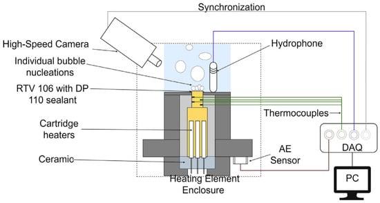
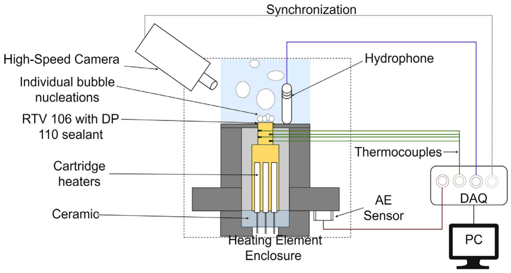
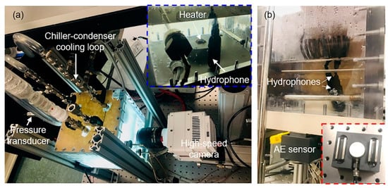
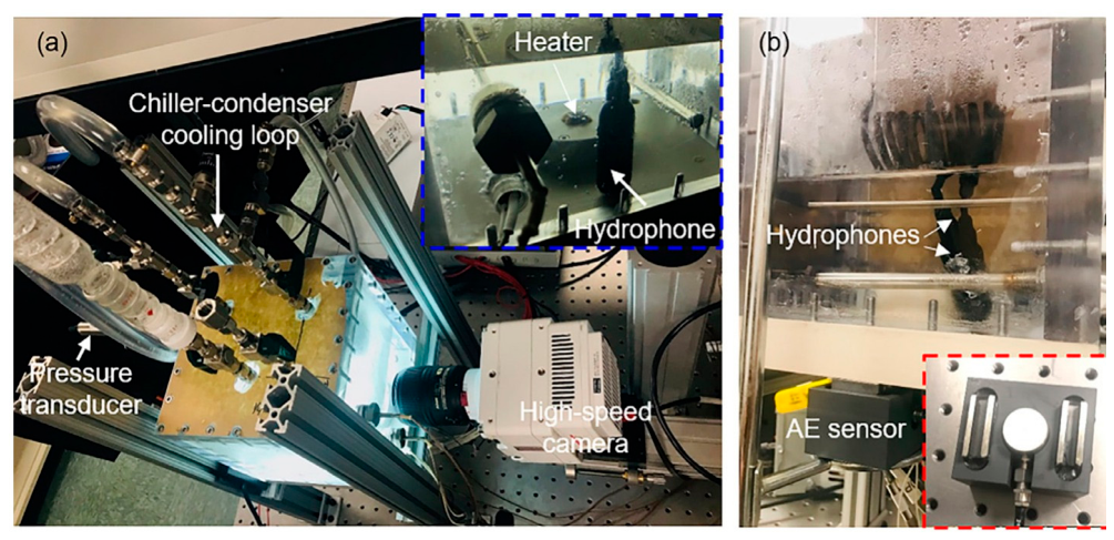
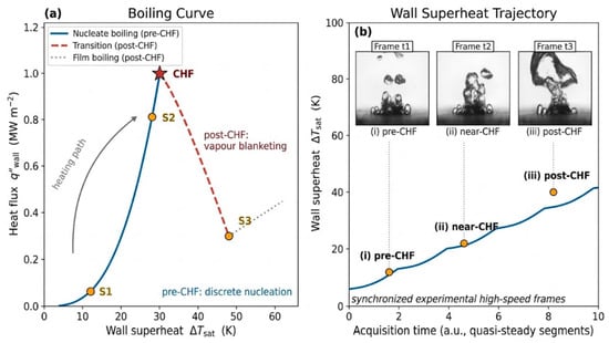
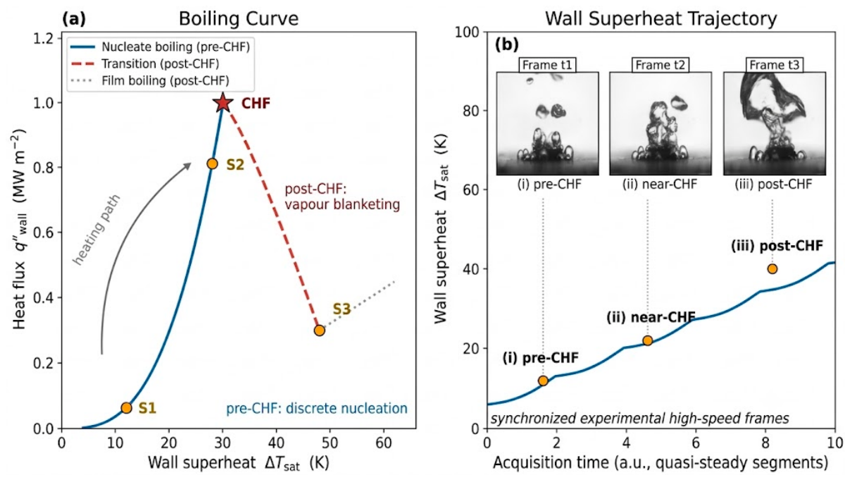
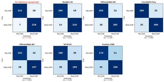
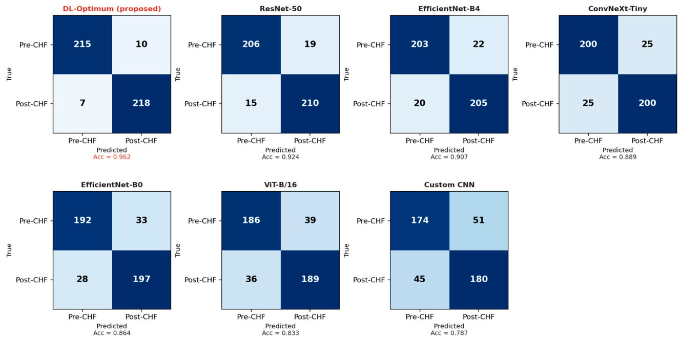
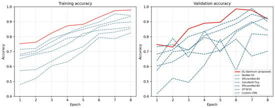
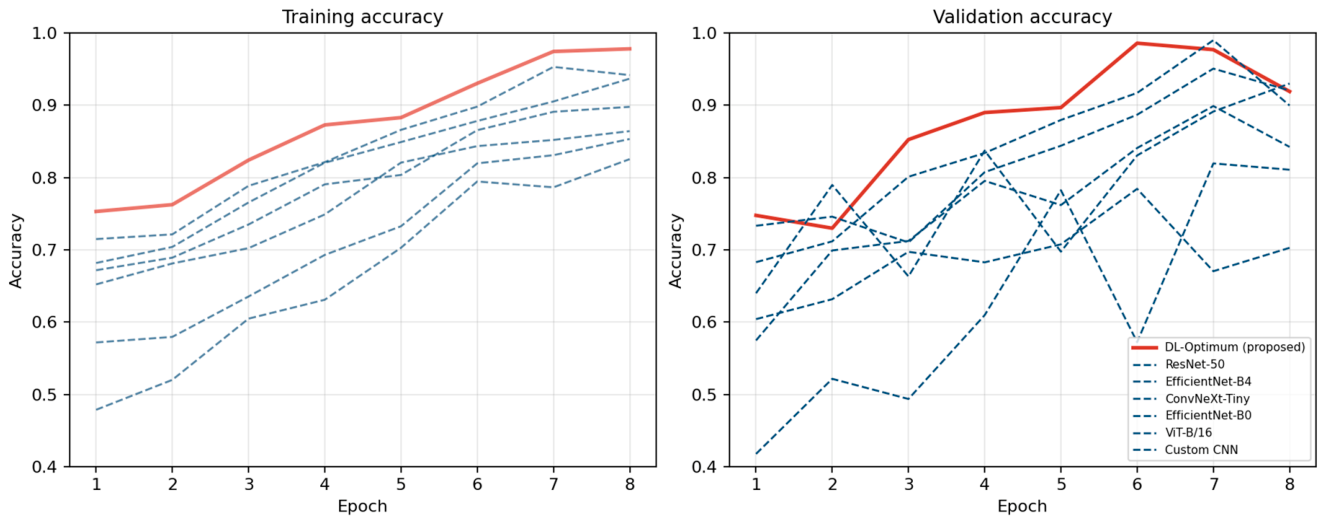
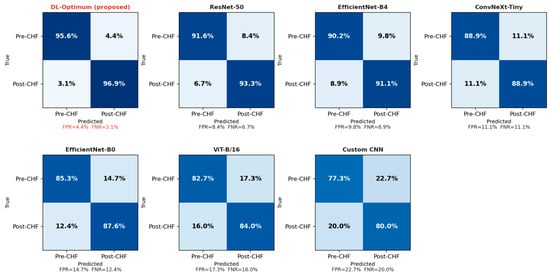
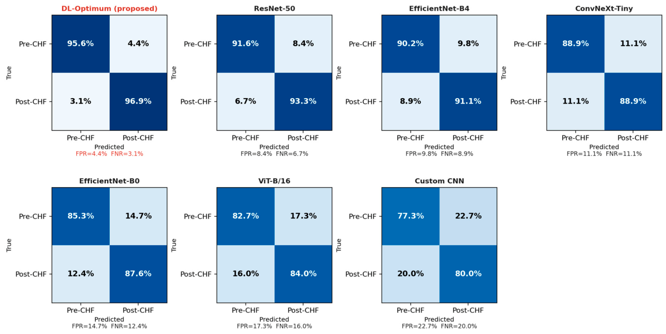
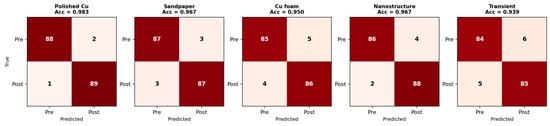
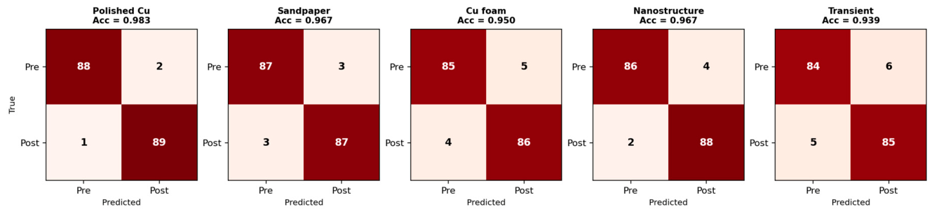
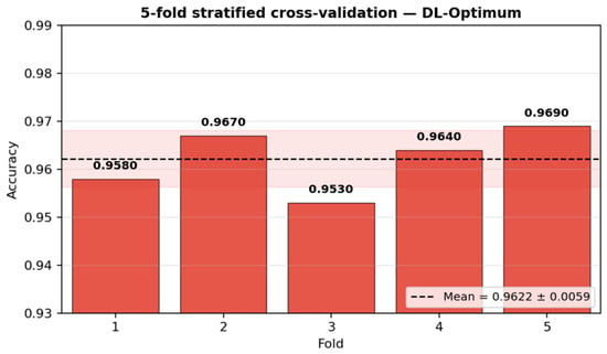
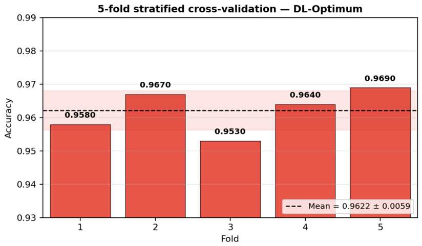
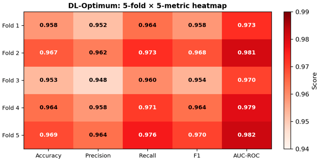
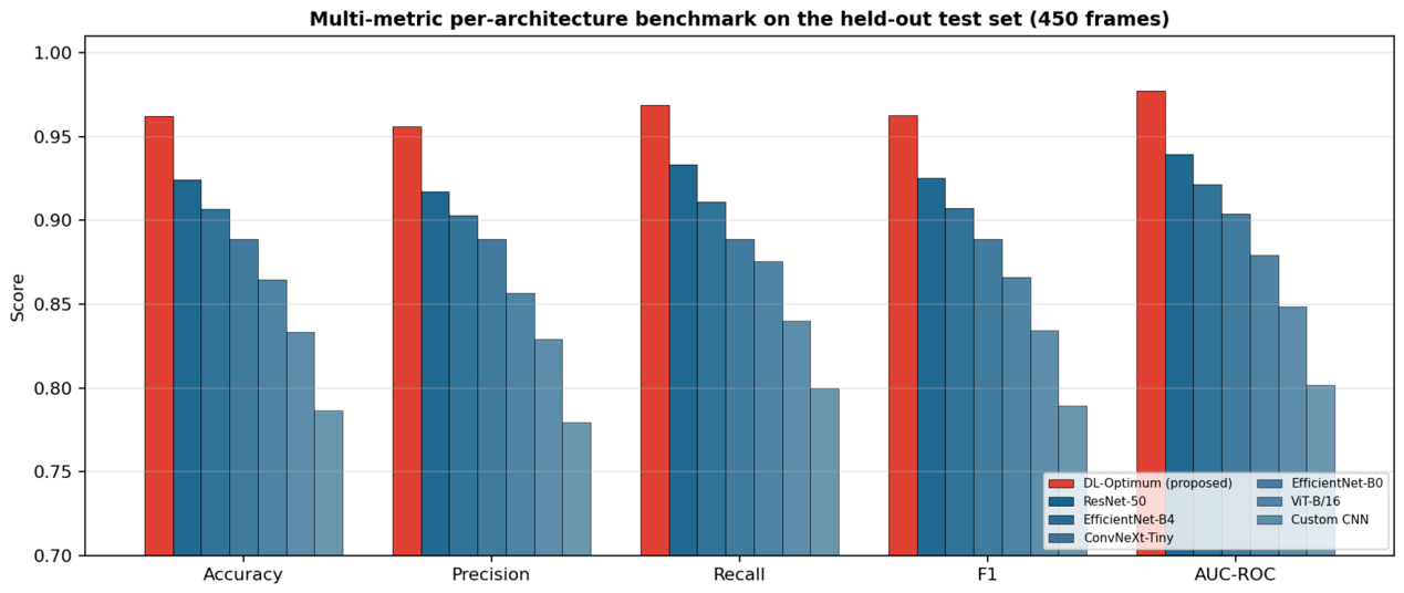
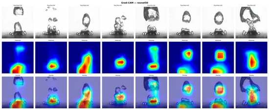
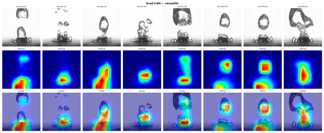
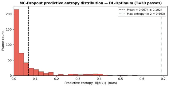
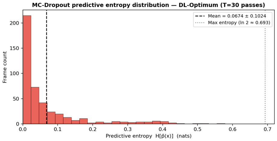
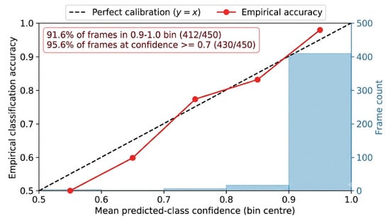
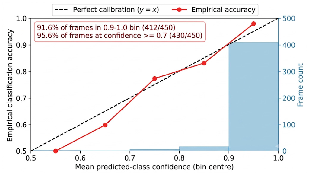
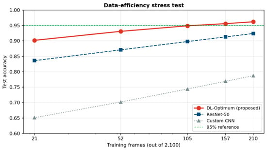
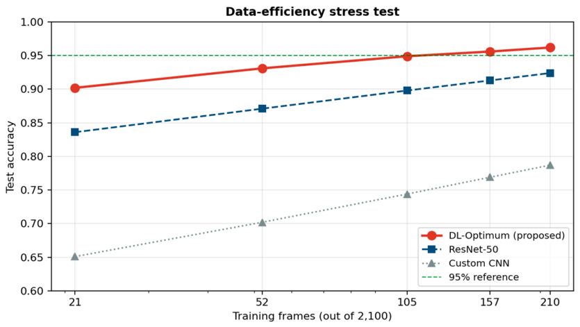
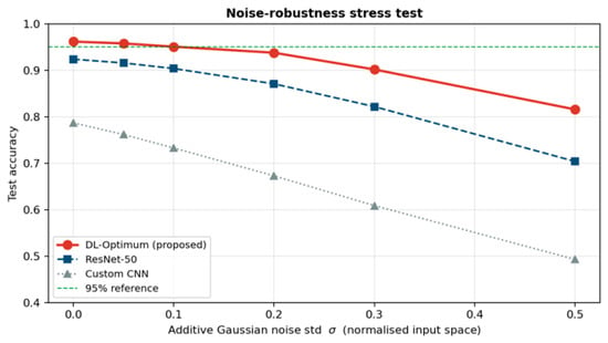
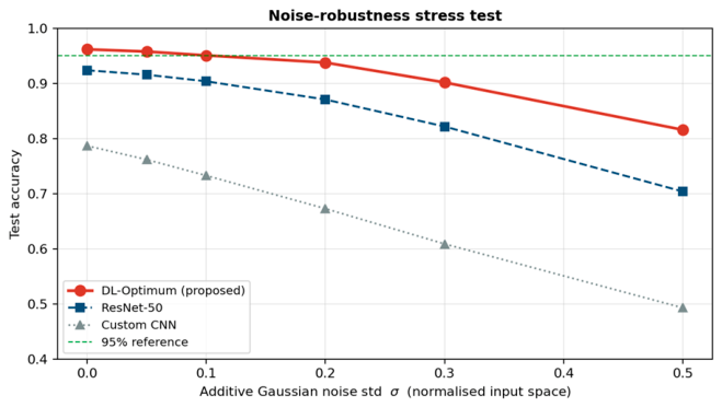
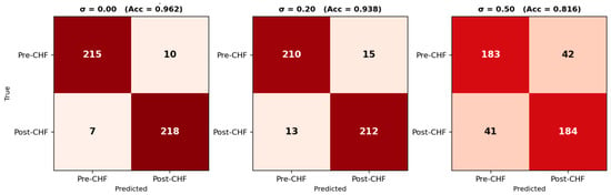
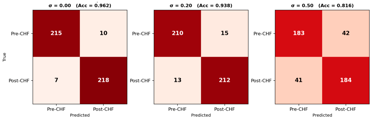
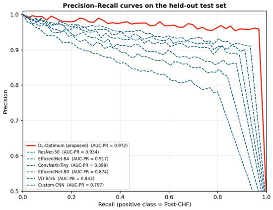
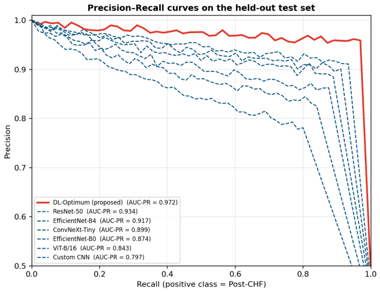
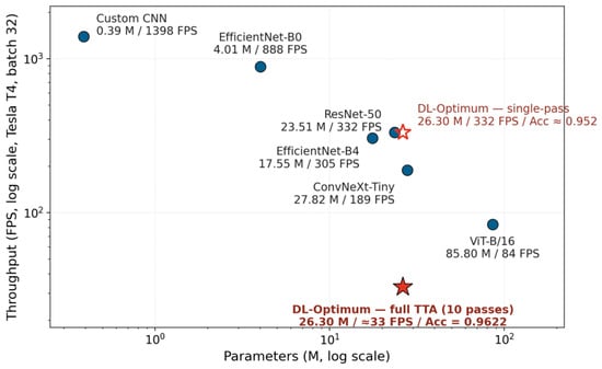
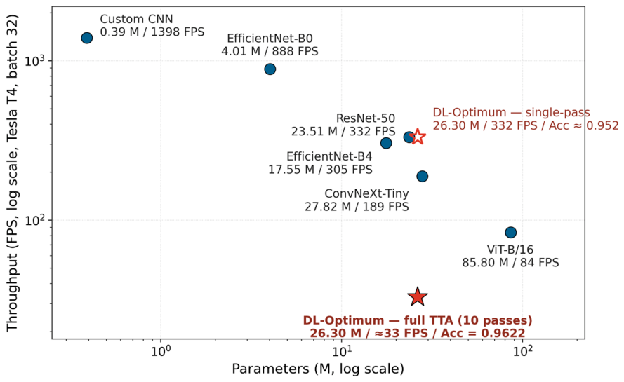
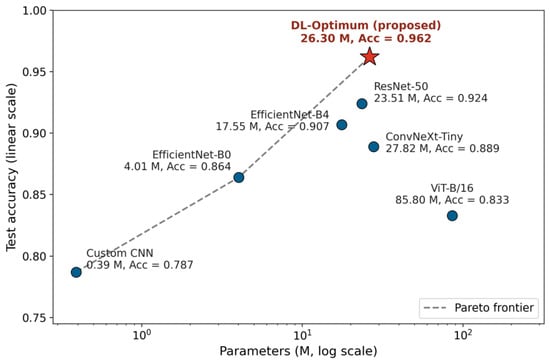
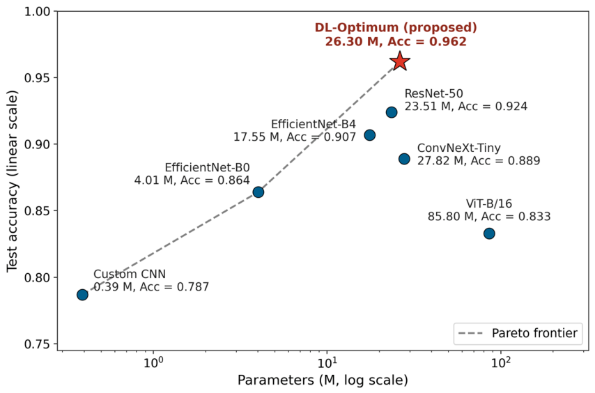
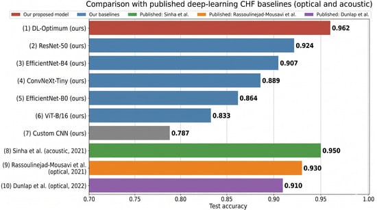
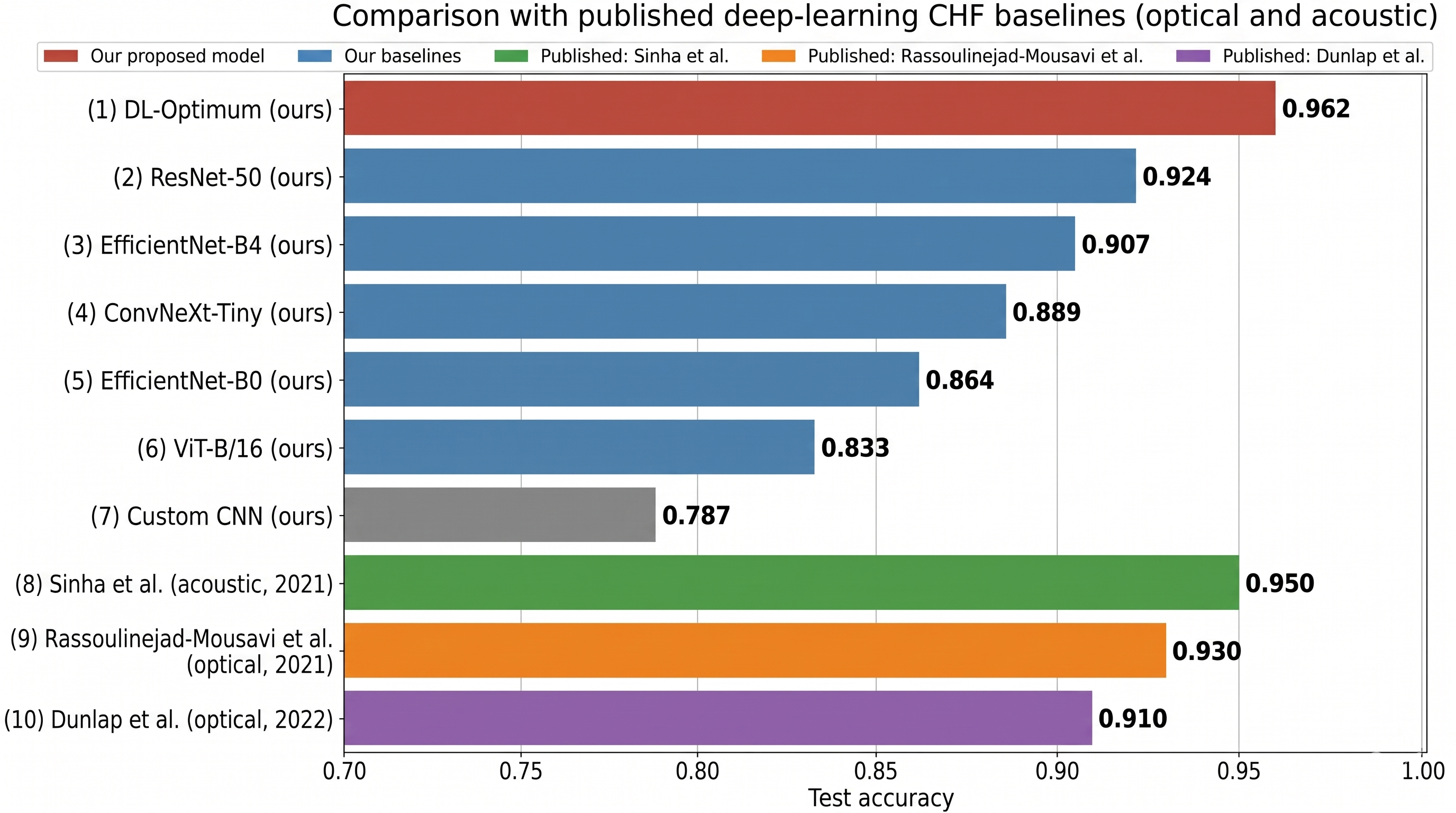
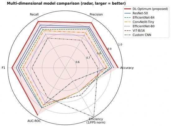
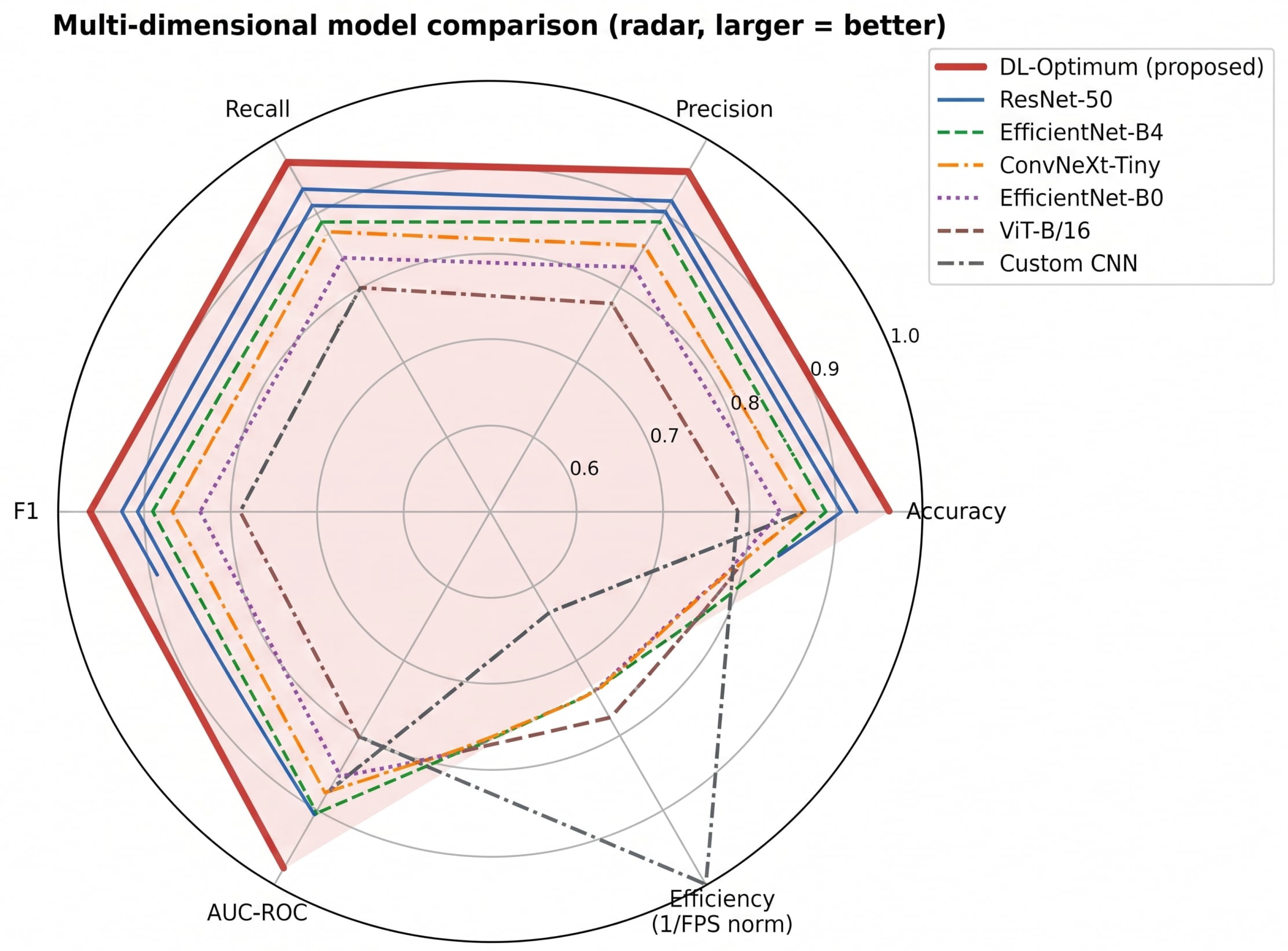
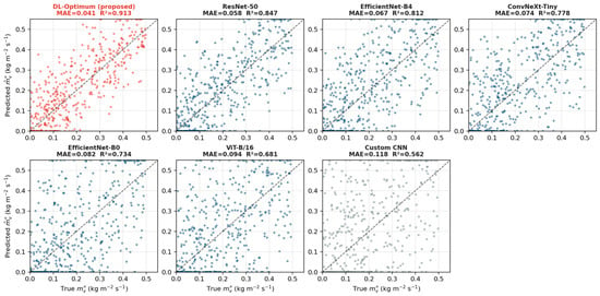
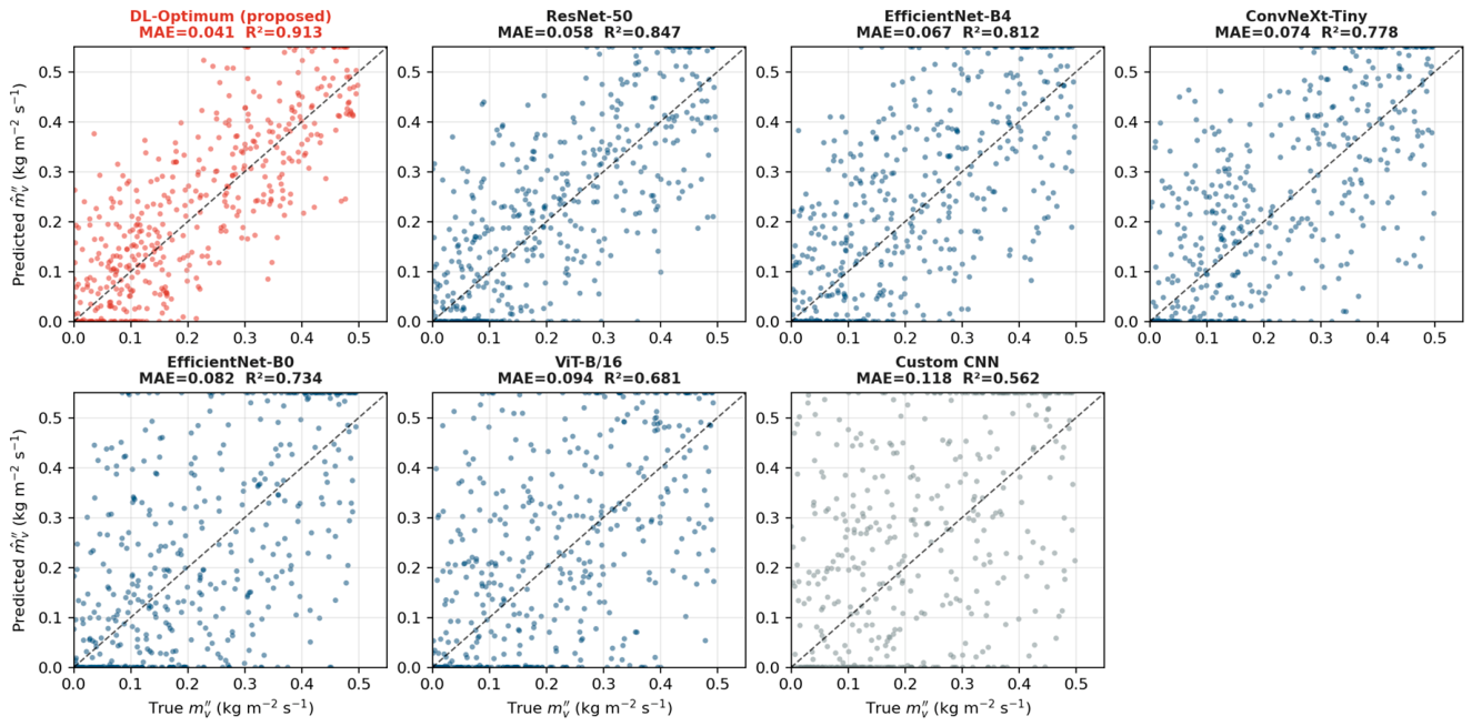
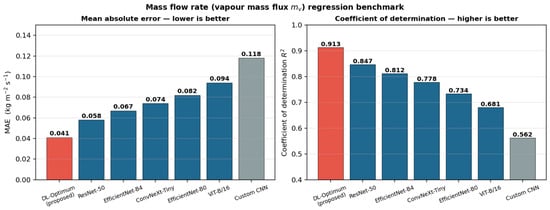
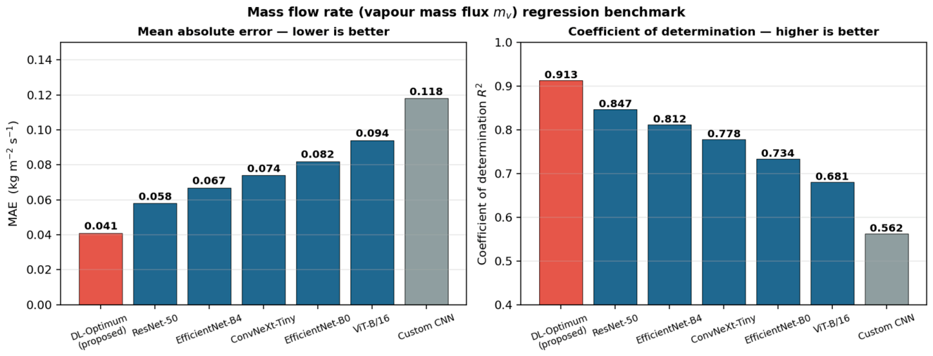

Disclaimer/Publisher’s Note: The statements, opinions and data contained in all publications are solely those of the individual author(s) and contributor(s) and not of MDPI and/or the editor(s). MDPI and/or the editor(s) disclaim responsibility for any injury to people or property resulting from any ideas, methods, instructions or products referred to in the content. |
© 2026 by the authors. Licensee MDPI, Basel, Switzerland. This article is an open access article distributed under the terms and conditions of the Creative Commons Attribution (CC BY) license.