A Physics-Constrained Probabilistic Forecasting Method for Wind–PV–Load Systems Under Extreme Weather Based on Extreme-Event Awareness and Uncertainty Calibration

Abstract

With the increasing penetration of renewable energy into power systems, wind and photovoltaic (PV) power generation exhibit substantial uncertainty due to meteorological variability, which becomes more pronounced under extreme weather conditions. The scarcity of extreme samples, complex dependencies among wind power, PV power, and load, and degraded prediction-interval reliability further increase the difficulty of probabilistic forecasting. To address these challenges, this study proposes a physics-constrained probabilistic forecasting framework for wind–PV–load systems under extreme weather. First, extreme value theory (EVT) is employed to characterize the tail behavior of meteorological variables, while extreme operating states are identified by jointly considering meteorological anomalies and renewable power responses. Second, a full-covariance mixture density network (MDN) is developed to model the joint probability distribution of wind power, PV power, and load while preserving their cross-variable dependencies. A physics-constrained Wasserstein generative adversarial network with gradient penalty (WGAN-GP) is then employed to generate multi-step wind–PV–load scenarios by incorporating operating, temporal, and cross-variable regularization. The historical and generated scenarios are subsequently used to train a long short-term memory (LSTM)-based quantile forecasting model, followed by conformalized quantile regression (CQR) for prediction-interval calibration. Experiments are conducted using wind power, PV power, load, and meteorological data from the Hai xi region of Qinghai Province, China, during 2021–2024. Results show that the full-covariance MDN effectively preserves the joint dependency structure, achieving a correlation reconstruction mean absolute error (MAE) of 0.032. The physics-constrained WGAN-GP substantially improves extreme-scenario generation quality. Meanwhile, LSTM+CQR achieves overall prediction interval coverage probability at a nominal 90% coverage level (PICP₉₀) values of 0.895 and 0.893 for PV and wind power, respectively, while under extreme weather the corresponding coverage reaches 0.704 and 0.635. The controlled augmentation experiment further shows improvements in extreme-weather forecasting accuracy and interval reliability. These results demonstrate that the proposed framework integrates extreme-state identification, joint uncertainty modeling, physics-constrained scenario generation, and uncertainty calibration for probabilistic renewable-power forecasting under extreme weather.

1. Introduction

With the increasing penetration of renewable energy, wind and photovoltaic (PV) power have become important components of modern power systems [1,2]. However, their strong dependence on meteorological conditions introduces substantial random-ness, variability, and intermittency, thereby increasing the uncertainty faced by power system operation [3,4,5,6]. The low occurrence frequency of extreme events also results in limited extreme samples, while complex dependencies among wind power, PV generation, and load further increase the difficulty of uncertainty modeling [7,8]. Such disturbances can further increase operational risks and challenge the resilience of power systems [9]. Moreover, distribution shifts caused by extreme weather may lead to insufficient prediction-interval coverage [10,11]. Therefore, probabilistic forecasting under extreme weather needs to address extreme-state identification, joint uncertainty modeling, extreme-sample scarcity, and prediction-interval reliability simultaneously.

Existing studies mainly identify extreme events using fixed thresholds, empirical quantiles, or extreme value theory (EVT) [12,13]. However, meteorological extremes do not necessarily correspond to abnormal renewable-energy operating states, and meteorological anomalies may produce different power responses under different operating conditions [14]. For uncertainty modeling, mixture density networks (MDNs) can characterize complex conditional probability distributions [15,16,17,18], but independent modeling or diagonal-covariance assumptions may neglect the dependencies among wind power, PV generation, and load. Generative adversarial networks (GANs) can alleviate the scarcity of extreme samples [19,20], but purely data-driven generation does not guarantee physical feasibility. Meanwhile, long short-term memory (LSTM)-based quantile forecasting can construct probabilistic prediction intervals [21,22,23], but may suffer from interval miscalibration under distribution shifts [24,25,26]. These limitations motivate the integration of extreme-state identification, joint probabilistic modeling, physics-constrained scenario generation, and prediction-interval calibration within a unified framework.

To address these challenges, this paper proposes a physics-constrained probabilistic forecasting framework for wind–PV–load systems under extreme weather, forming a complete technical chain of “extreme-state identification—joint uncertainty modeling—extreme-scenario augmentation—probabilistic forecasting—prediction-interval calibration.” First, EVT is employed to characterize the tail behavior of meteorological variables, while extreme operating states are identified by jointly considering meteorological anomalies and renewable power responses. Second, a full-covariance MDN is developed to model the joint probability distribution of wind power, PV generation, and load while preserving their dependency structure. A physics-constrained Wasserstein generative adversarial network with gradient penalty (WGAN-GP) is then employed to generate multi-step wind–PV–load scenarios, with operating-bound, net-balance, meteorology–power, temporal, and cross-variable regularization incorporated to improve trajectory-level consistency. Finally, an LSTM-based quantile model is used for probabilistic forecasting, followed by conformalized quantile regression (CQR) to calibrate the prediction intervals.

Experiments are conducted using wind power, PV generation, load, and meteorological data from the Hai xi region of Qinghai Province, China, during 2021–2024. The results demonstrate that the proposed framework can effectively characterize joint dependencies, improve prediction-interval reliability, and enhance downstream forecasting performance under extreme weather. The full-covariance MDN achieves a correlation reconstruction mean absolute error (MAE) of 0.032, while LSTM+CQR attains overall prediction interval coverage probability at a nominal 90% coverage level (PICP₉₀) values of 0.895 and 0.893 for PV and wind power, respectively. Under a controlled computational budget, GAN-based augmentation reduces the extreme-weather PV root mean square error (RMSE) from 0.0699 to 0.0567 and the wind-power RMSE from 0.0939 to 0.0823, while improving the corresponding prediction-interval coverage. These results support the complementary roles of dependency modeling, scenario augmentation, and uncertainty calibration in extreme-weather probabilistic forecasting.

2. Methodology

2.1. Framework Overview

Extreme weather can introduce stronger nonlinear, nonstationary, and uncertain characteristics into renewable power forecasting. Since extreme events account for only a small proportion of historical samples, directly training a unified forecasting model on all available data may be dominated by normal operating samples and thus weaken the representation of extreme operating states. To address this issue, this study develops a staged forecasting framework following the sequence of “state identification—joint probabilistic modeling—extreme-scenario augmentation—probabilistic forecasting and calibration.” Each stage is designed to address a specific challenge associated with extreme-weather forecasting.

First, EVT is applied to characterize the tail behavior of meteorological and operating variables. Candidate extreme-weather states are then identified through a dual-path strategy that combines event-specific meteorological criteria with the corresponding renewable-energy responses using an AND rule. The resulting state labels are then used to distinguish normal and extreme operating conditions. Subsequently, a joint probabilistic model is established for wind power, PV generation, and load, where a full-covariance structure is retained to preserve their dependency relationships and provide a joint uncertainty basis for subsequent scenario generation. The resulting mixture-component statistics, together with the extreme-state encoding, provide conditional information for the subsequent scenario-generation model.

To alleviate the scarcity of extreme-weather samples, a physics-constrained WGAN-GP is employed to generate multi-step wind–PV–load trajectories. In addition to adversarial distribution learning, event-conditioned operating bounds, net-balance consistency, meteorology–power consistency, ramp characteristics, lag-one temporal dependence, and cross-variable dependence are incorporated as soft regularization terms. These constraints are used to improve the temporal and operational consistency of the generated trajectories while retaining sample diversity. The generated scenarios are subsequently used to augment the training data for probabilistic forecasting.

For probabilistic forecasting, an LSTM-based quantile model is employed to capture temporal dependencies in historical observations and generate multi-horizon quantile forecasts for wind and PV power. CQR is further applied to calibrate the resulting prediction intervals and correct coverage deviations under different weather conditions, thereby improving interval reliability.

Overall, the proposed framework establishes a complete methodological chain from extreme-state identification and joint uncertainty modeling to extreme-scenario augmentation, probabilistic forecasting, and prediction-interval calibration. Information is progressively transferred between successive modules to jointly address state heterogeneity, variable dependency, extreme-sample scarcity, and prediction-interval miscalibration under extreme weather. Detailed descriptions of the four modules are provided in Section 2.2, Section 2.3, Section 2.4 and Section 2.5.

2.2. EVT-GPD-Guided Dual-Path Extreme-State Identification

Extreme weather events are characterized by low occurrence frequencies and pronounced tail behavior, whereas meteorological extremes do not necessarily induce abnormal operating responses in renewable-energy systems. Therefore, relying on either statistical tail information or a single deterministic threshold alone may be insufficient to distinguish meteorological extremes that have actual operational impacts. To address this issue, an EVT-Generalized Pareto Distribution (GPD)-guided dual-path identification framework is adopted. In this framework, EVT-GPD analysis is first used to characterize the tail behavior of meteorological and operating variables and to provide statistical support for extreme-threshold selection. The final event labels are then determined by jointly considering event-specific meteorological criteria and the corresponding responses of wind power, PV generation, and load through an AND fusion rule. The overall procedure consists of tail modeling, meteorological extreme detection, renewable-response detection, and dual-path fusion.

2.2.1. EVT-GPD Tail Modeling

EVT is employed to characterize the tail behavior of meteorological and operating variables. For an observed variable X, the peak over threshold (POT) approach is adopted by selecting a sufficiently high threshold u. For an upper-tail event, the exceedances over the threshold are defined as:

$$\begin{array}{cc}Y=X-u,& X>u\end{array}$$

(1)

According to the Pickands–Balkema–de Haan (PBH) theorem, when the threshold u is sufficiently high, the conditional distribution of exceedances can be approximated by a GPD:

$$G_{\mathit{\xi },\mathit{\sigma }}(y)=\left\{\begin{array}{l}\begin{array}{cc}1-{\left(1+{\displaystyle \frac{\mathit{\xi y}}{\sigma }}\right)}^{-1/\xi },& \xi \ne 0\end{array}\\ \begin{array}{cc}1-\exp \left(-{\displaystyle \frac{y}{\sigma }}\right),& \xi =0\end{array}\end{array}\right.$$

(2)

where y denotes the exceedances, σ > 0 is the scale parameter, and ξ is the shape parameter. A positive ξ indicates a heavy tail, ξ ≈ 0 corresponds to an approximately exponential tail, and ξ < 0 indicates a bounded tail.

For lower-tail variables, such as low temperature or low PV output, the sign of the original variable is reversed before applying the same upper-tail POT procedure:

X^∗ = −X

(3)

In the implementation, the initial POT is set to the empirical 90th percentile of the transformed variable. GPD parameters are estimated by maximum likelihood using the Nelder–Mead optimization algorithm, with ξ₀ = 0 and σ₀ = std(Y) as the initial values and a maximum of 1000 iterations. A GPD fit is retained only when at least 20 exceedances are available. To examine threshold sensitivity, additional POT fits are evaluated over empirical quantiles from 0.85 to 0.95. In the proposed framework, EVT-GPD analysis is used to characterize tail behavior and support threshold selection, rather than to serve as the sole rule for assigning final extreme-event labels.

2.2.2. Event-Specific Meteorological-Threshold Path

Following the EVT-GPD tail analysis, event-specific meteorological criteria are used to screen candidate extreme-weather states. Rather than applying a single common threshold to all meteorological variables, the thresholds are defined according to the physical characteristics of each weather category. Specifically, a cold-wave candidate is identified when the daily temperature satisfies T ≤ −15 °C; a snowstorm candidate requires daily precipitation of at least 10 mm; a sandstorm-like candidate is represented by a low-humidity and high-wind proxy, with relative humidity RH ≤ 20% and maximum wind speed WS_max ≥ 10 m/s; a high-wind candidate requires WS_max ≥ 17 m/s; and a heat-wave candidate requires the daily maximum temperature to satisfy T_max ≥ 35 °C. For event category k, the meteorological-path indicator is defined as

$$M_k\left(t\right)=\mathbb{I}[m_t\in {\Omega }_k^{\mathrm{met}}]$$

(4)

where m_t denotes the meteorological observations at time t, ${\Omega }_k^{\mathrm{met}}$ denotes the event-specific meteorological criterion, and 𝕀[⋅] is the indicator function.

These meteorological thresholds constitute the first identification path and are subsequently combined with event-specific renewable-energy response criteria.

2.2.3. Renewable-Response Verification Path

Meteorological extremes do not necessarily result in abnormal renewable-energy operation. Therefore, a second identification path is introduced to verify whether the candidate meteorological event is accompanied by a corresponding change in wind power, PV generation, or load. Rather than using a single standardized anomaly threshold for all operating variables, event-specific empirical quantiles are adopted to characterize the relevant renewable-energy responses.

Specifically, a high-load response is defined as Load ≥ P₉₀, which is used to verify cold-wave and heat-wave candidates. For snowstorm and sandstorm-like candidates, a low-PV response is defined as PV ≤ P₁₅. For high-wind events, abnormal wind-power fluctuation is characterized by the daily standard deviation of normalized wind power, with σ_wind ≥ P₉₅. Persistent low-radiation conditions are identified when normalized PV output satisfies PV ≤ P₁₀ on at least two days within a three-day rolling window.

For event category k, the renewable-response indicator is expressed as

$$R_k\left(t\right)=\mathbb{I}[y_t\in {\Omega }_k^{\mathrm{resp}}]$$

(5)

where y_t denotes the operating variables at time t, ${\Omega }_k^{\mathrm{resp}}$ denotes the event-specific renewable-response criterion, and 𝕀[⋅] is the indicator function. This response-verification path ensures that the final extreme-event label reflects not only anomalous meteorological conditions but also their observable operational impacts.

2.2.4. Dual-Path and Fusion

The final event label is determined by jointly combining the meteorological-threshold path and the renewable-response verification path through an AND rule. For event category k, the fused extreme-event indicator is defined as:

E_k(t) = M_k(t) ∧ R_k(t)

(6)

where M_k(t) and R_k(t) denote the meteorological and renewable-response indicators, respectively. Therefore, a candidate event is confirmed only when both the event-specific meteorological condition and its corresponding operational-response criterion are satisfied. Using this strategy, six categories of extreme weather events are identified:

Cold Wave: T ≤ −15 °C ∩ Load ≥ P₉₀

Snowstorm: Precip ≥ 10 mm ∩ PV ≤ P₁₅

Sandstorm: RH ≤ 20%, WSmax ≥ 10 m/s ∩ PV ≤ P₁₅

High Wind: WS_max ≥ 17 m/s ∩ σ_wind ≥ P₉₅

Heat Wave: T_max ≥ 35 °C ∩ Load ≥ P₉₀

Low Radiation: PV ≤ P₁₀ on at least two days within a three-day rolling window

Since different event criteria may be satisfied on the same day, the resulting labels are allowed to be multi-label. Accordingly, the sum of event-category occurrences can exceed the number of unique extreme-weather days. The final extreme-state indicator is defined as

$$E\left(t\right)=\mathbb{I}[{\displaystyle \sum _k{E}_k\left(t\right)>0}]$$

(7)

where E(t) indicates that at least one extreme-event criterion is satisfied. These labels are subsequently used to distinguish normal and extreme samples in the downstream joint probabilistic modeling, scenario-generation, and forecasting stages.

2.3. Full-Covariance MDN for Joint Probabilistic Characterization

Wind power, PV generation, and load are jointly affected by meteorological conditions and system operating states and therefore exhibit non-negligible cross-variable dependence. Modeling the three variables independently may fail to represent their coordinated uncertainty. To characterize their joint probabilistic behavior, a full-covariance MDN is constructed to estimate the conditional joint distribution of wind power, PV generation, and load. Let

$$y_t={\left[W_t,P_t,L_t\right]}^T$$

(8)

denote the three-dimensional target vector and c_t denote the corresponding conditioning vector. The conditional density is represented by a mixture of K multivariate Gaussian components:

$$p(y_t|x_t)={\displaystyle \sum _{k=1}^K{\pi }_k(}{c}_t)\mathcal{N}(y_t|{\mu }_k(c_t),{\Sigma }_k(c_t))$$

(9)

where π_k, μ_k, and Σ_k denote the mixture weight, mean vector, and covariance matrix of the k-th component, respectively, with

$$\begin{array}{cc}{\pi }_k>0& \begin{array}{cc},& {\displaystyle \sum _{k=1}^K{\pi }_k=1}\end{array}\end{array}$$

(10)

2.3.1. Full-Covariance Parameterization

To explicitly represent dependence among wind power, PV generation, and load, each Gaussian component retains a full 3 × 3 covariance matrix rather than assuming diagonal covariance. To guarantee positive definiteness, the covariance matrix is parameterized by Cholesky decomposition:

$${\Sigma }_k=L_k{L}_k^T$$

(11)

where L_k is a lower-triangular matrix. The diagonal elements of L_k are transformed using

L_k,ii = softplus(a_k,ii) + 10⁻⁴

(12)

ensuring strictly positive diagonal entries and improving numerical stability. The mixture weights are obtained using a softmax transformation, while the component means are constrained to the normalized output range using a sigmoid transformation.

2.3.2. Network Architecture and Training Objective

The conditioning vector is processed by a shared fully connected feature extractor. The implemented network contains hidden layers with 128, 128, 64, and 64 units, respectively. Each hidden layer uses Gaussian error linear unit (GELU) activation, batch normalization, and a dropout rate of 0.1. The final MDN layer outputs the mixture probabilities, three-dimensional component means, and six independent elements of the lower-triangular Cholesky factor for each component.

The basic training objective is the negative log-likelihood (NLL):

$${\mathcal{L}}_{\mathrm{NLL}}=-{\displaystyle \frac{1}{N}}{\displaystyle \sum _{i=1}^N\log }\left[{\displaystyle \sum _{k=1}^K{\pi }_{\mathit{ik}}}\mathcal{N}\left(y_i|{\mu }_{\mathit{ik}},{\Sigma }_{\mathit{ik}}\right)\right]$$

(13)

To additionally encourage consistency of the predicted cross-variable dependence with the empirical dependence within a training batch, a correlation regularization term is included:

$ℒ$_MDN = $ℒ$_NLL + λ_corr$ℒ$_corr,

(14)

where λ_corr = 0.15 in the implemented configuration.

2.3.3. Mixture-Component Selection and Training Settings

The number of Gaussian mixture components is selected from

K ∈ {1,3,5,7}

(15)

All candidate models use the same input features, data partition, feature transformation, and network backbone, with only the MDN output dimension changing with K. Model selection is based primarily on validation negative log-likelihood, and K = 5 is retained for the subsequent analysis. The model is optimized using Adam with a learning rate of 1 × 10⁻³ and a batch size of 64. A fixed random seed is used for reproducibility.

2.4. Physics-Constrained WGAN-GP for Multi-Step Extreme-Scenario Generation

Extreme-weather events usually occur with low frequency, resulting in limited historical samples and insufficient representation of rare operating states. To increase the diversity of extreme-weather samples while maintaining the temporal and operational characteristics of wind–PV–load systems, a conditional WGAN-GP is employed to generate multi-step joint trajectories of wind power, PV power, and load [27,28].

The model combines adversarial distribution learning with event-conditioned operating constraints, net-balance consistency, meteorology–power consistency, temporal regularization, and cross-variable dependence regularization. These constraints are incorporated as differentiable soft penalties in the generator objective so that the generated trajectories maintain sample diversity while reducing unrealistic temporal and operational behavior.

2.4.1. Conditional Input and Multi-Step Output

For each generated trajectory, the conditional vector is constructed as

$$c=\left[e,\mathrm{vec}\left({\mu }_1,\dots ,{\mu }_5\right),\overline{\sigma }\right]$$

(16)

where e ∈ ℝ⁷ is a one-hot encoding of the normal state and six extreme-event categories. vec(μ) ∈ ℝ¹⁵ contains the mean vectors of the five Gaussian components predicted by the full-covariance MDN, and $\overline{\sigma }\in {ℝ}^3$ contains the component-averaged marginal standard deviations derived from the Cholesky covariance factors.

Given the latent vector z ∈ ℝ⁶⁴, the generator produces

$$\widehat{Y}=G(z,c)\in {[0,1]}^{H\times 3}$$

(17)

where H = 16 represents sixteen consecutive 15 min steps, corresponding to a 4 h scenario horizon, and the three output channels correspond to wind power, PV power, and load.

2.4.2. WGAN-GP Objective and Physics-Informed Constraints

The critic is trained using the Wasserstein objective with gradient penalty,

$${\mathcal{L}}_D=\mathbb{E}[D(\widehat{Y},c)]-\mathbb{E}[D(Y,c)]+{\lambda }_{\mathit{GP}}\mathbb{E}\left[{\left({‖{\nabla }_{\tilde{Y}}D(\tilde{Y},c)‖}_2-1\right)}^2\right]$$

(18)

where the gradient-penalty coefficient is set to λ_GP = 10.

Five critic updates are performed for each generator update. The latent dimension is 64, the conditional dimension is 25, the output dimension is 3, and the batch size is 64. Adam is used for both networks, with generator and critic learning rates of 5 × 10⁻⁵ and 2 × 10⁻⁴, respectively, and β₁ = 0.5, β₂ = 0.9.

The adversarial component of the generator loss is

$${\mathcal{L}}_{\mathit{adv}}=-\mathbb{E}[D(\widehat{Y},c)]$$

(19)

In addition to the adversarial term, several soft constraints are introduced to characterize the operating and temporal properties of the generated trajectories.

For event category k, variable j, and scenario step h, the event-conditioned operating-bound penalty is defined as

$${\mathcal{L}}_{\mathit{bound}}={\displaystyle \frac{1}{3H}}{\displaystyle \sum _{h=1}^H{\displaystyle \sum _{j=1}^3\left[\mathrm{ReLU}{(l_{k,j}-{\widehat{y}}_{h,j})}^2+\mathrm{ReLU}{({\widehat{y}}_{h,j}-u_{k,j})}^2\right]}}$$

(20)

where l_k,j and u_k,j denote the lower and upper operating bounds of variable j under event category k. No additional penalty is imposed when the generated value remains within the corresponding interval.

To characterize the balancing requirement of the wind–PV–load system without assuming instantaneous equality between renewable generation and load, the net-balance residual is defined as

r_h = L_h − W_h − P_h

(21)

This residual represents the balancing requirement that may be supplied or absorbed by other system resources, including conventional generation, storage, external grid exchange, and system losses. For each event category, empirical lower and upper residual limits $r_k^L$ and $r_k^U$ are determined from the training data. The corresponding penalty is

$${\mathcal{L}}_{\mathit{bal}}={\displaystyle \frac{1}{H}}{\displaystyle \sum _{h=1}^H\left[\mathrm{ReLU}{(r_k^L-{\widehat{r}}_h)}^2+\mathrm{ReLU}{({\widehat{r}}_h-r_k^U)}^2\right]}$$

(22)

Meteorology–power consistency is characterized using the meteorological variables available in the dataset. Wind-power behavior is associated with the mean wind-speed variable, whereas PV output is associated with sunshine duration as the solar-resource indicator. The training samples are divided into empirical meteorological quantile bins, and the P₅–P₉₅ range of the corresponding power output within each bin is used to construct a weather-conditioned operating envelope.

For generated power ${\widehat{p}}_h$, the corresponding penalty is

$${\mathcal{L}}_{\mathit{met}}={\displaystyle \frac{1}{H}}{\displaystyle \sum _{h=1}^H\left[\mathrm{ReLU}{(p^L(m)-{\widehat{p}}_h)}^2+\mathrm{ReLU}{({\widehat{p}}_h-p^U(m))}^2\right]}$$

(23)

where p^L(m) and p^U(m) denote the lower and upper empirical power limits under meteorological condition m. The wind-speed–wind-power and solar-resource–PV penalties are averaged to form the meteorology–power consistency term.

Temporal continuity is characterized using ramp statistics and lag-one autocorrelation. For variable j, the mean absolute ramp is defined as

$$R_j(Y)={\displaystyle \frac{1}{H-1}}{\displaystyle {\displaystyle \sum _{h=2}^H}|}{y}_{h,j}-y_{h-1,j}|$$

(24)

The ramp regularization term is

$${\mathcal{L}}_{\mathit{ramp}}={\displaystyle \frac{1}{3}}{\displaystyle \sum _{j=1}^3\frac{|R_j(\widehat{Y})-R_j(Y)|}{R_j(Y)+ϵ}}$$

(25)

The lag-one temporal correlation penalty is defined as

$${\mathcal{L}}_{\mathit{lag}}={\displaystyle \frac{1}{3}}{\displaystyle \sum _{j=1}^3\left|{\rho }_j^{(1)}(\widehat{Y})-{\rho }_j^{(1)}(Y)\right|}$$

(26)

where ${\rho }_j^{(1)}$ denotes the lag-one Pearson correlation coefficient of variable j.

Cross-variable dependence among wind power, PV power, and load is further characterized through the three pairwise Pearson correlation coefficients:

$${\mathcal{L}}_{\mathit{cross}}={\displaystyle \frac{1}{3}}{\displaystyle \sum _{(i,j)\in \{(W,P),(W,L),(P,L)\}}\left|{\rho }_{\mathit{ij}}(\widehat{Y})-{\rho }_{\mathit{ij}}(Y)\right|}$$

(27)

The complete generator objective is therefore

$ℒ$_G = $ℒ$_adv + λ_b$ℒ$_bound + λ_bal$ℒ$_bal + λ_met$ℒ$_met + λ_r$ℒ$_ramp + λ_l$ℒ$_lag + λ_c$ℒ$_cross

(28)

The loss weights are set to λ_b = 8, λ_bal = 0.1, λ_met = 0.1, λ_r = 0.5, λ_l = 1, λ_c = 1.

All empirical operating bounds, residual limits, and meteorology–power envelopes are estimated using the training partition only. These terms are implemented as soft regularization rather than hard feasibility constraints. Therefore, they characterize trajectory-level operating consistency but do not represent complete storage-state dynamics, network power-flow feasibility, or other unobserved system constraints.

2.5. LSTM-Based Quantile Forecasting and CQR Calibration

Extreme weather can increase both forecasting errors and prediction-interval miscalibration. Therefore, the forecasting stage is formulated as a multi-horizon quantile regression problem rather than a deterministic point-forecasting task [29,30]. An LSTM-based model is used to extract temporal dependencies from historical operating and meteorological features and to simultaneously predict multiple quantiles of future PV and wind power. CQR is subsequently applied as a post-processing step to calibrate the nominal prediction intervals without retraining the forecasting network.

2.5.1. Forecasting Sample Construction and LSTM Architecture

The forecasting task uses a sliding-window formulation. Each input sample contains the preceding 96 time steps of 15 min observations, corresponding to a 24 h historical window, and the model predicts the subsequent 16 time steps, corresponding to a 4 h forecasting horizon. Each historical time step contains 25 input features, and the forecasting targets are normalized PV and wind power.

The resulting input and output tensors are

X_t ∈ ℝ^96×25

(29)

Y_t ∈ ℝ^16×2

(30)

The LSTM quantile network consists of a 64-unit LSTM layer with return_sequences = True, followed by a dropout layer with a rate of 0.20, a second 32-unit LSTM layer, and another dropout layer with a rate of 0.20. The extracted temporal representation is passed through a 512-unit fully connected layer with rectified linear unit (ReLU) activation and batch normalization, followed by a 160-unit output layer. The output is reshaped to 16 × 2 × 5, corresponding to 16 forecasting horizons, two target variables, and five quantile levels. The complete model contains 136,480 parameters.

2.5.2. Quantile Regression and Training Objective

Five conditional quantiles are predicted simultaneously:

Q = {0.05,0.25,0.50,0.75,0.95}

(31)

For an observation y, predicted quantile ${\widehat{y}}_q$, and quantile level q, the pinball loss is defined as

$${\rho }_q(y,{\widehat{y}}_q)=\left\{\begin{array}{ll}q(y-{\widehat{y}}_q),\hfill & y\ge {\widehat{y}}_q\hfill \\ (q-1)(y-{\widehat{y}}_q),\hfill & y<{\widehat{y}}_q\hfill \end{array}\right.$$

(32)

The training loss is obtained by averaging the quantile losses over forecasting horizons, target variables, and quantile levels. To increase the contribution of rare extreme-weather samples during model fitting, extreme windows are assigned a sample weight of 8 relative to normal windows.

To prevent quantile crossing, the raw network outputs are transformed using cumulative positive increments:

$${\widehat{q}}_1=b,{\widehat{q}}_j=b+{\displaystyle \sum _{r=2}^j\mathrm{softplus}}(a_r),j=2,\dots ,5$$

(33)

followed by the output-range transformation used for the normalized targets. This construction enforces ${\widehat{q}}_{0.05}\le {\widehat{q}}_{0.25}\le {\widehat{q}}_{0.50}\le {\widehat{q}}_{0.75}\le {\widehat{q}}_{0.95}$.

The network is optimized using Adam with a learning rate of 10⁻³, β₁ = 0.9, β₂ = 0.999, ϵ = 10⁻⁷, and a batch size of 128.

2.5.3. CQR Calibration

CQR is applied to the nominal 90% interval formed by the 0.05 and 0.95 quantiles. To preserve the representation of extreme and normal operating conditions in both calibration and evaluation, the test windows are first separated according to their extreme-event indicator [31]. Half of each group is assigned to the calibration subset and the remaining half to the evaluation subset; the selected indices are then restored to their original temporal order within each subset.

For target variable v, the conformity score is

$$s_i^{(v)}=\max \left\{{\widehat{q}}_{0.05,i}^{(v)}-y_i^{(v)},y_i^{(v)}-{\widehat{q}}_{0.95,i}^{(v)}\right\}$$

(34)

Scores from all 16 forecast horizons are pooled separately for each target variable. For a nominal coverage level 1 − α = 0.90, the correction constant is taken as the k = [(n + 1)(1 − α)]-th ordered conformity score, with k truncated to n when necessary. The calibrated interval is then $\left[\max (0,{\widehat{q}}_{0.05}-{\delta }_v),\min (1,{\widehat{q}}_{0.95}+{\delta }_v)\right]$.

A separate correction constant δ_v is estimated for PV and wind power. CQR is used only to recalibrate the interval bounds; the median forecast remains unchanged.

2.6. Evaluation Metrics and Statistical Uncertainty

To evaluate forecasting performance from complementary perspectives, deterministic accuracy, prediction-interval reliability and sharpness, and overall probabilistic forecast quality are considered. RMSE and MAE are used for point-forecast accuracy; PICP, mean prediction interval width (MPIW), and absolute coverage error (ACE) jointly evaluate interval coverage and sharpness; and continuous ranked probability score (CRPS) evaluates probabilistic distribution quality. Metrics are reported separately for PV and wind power and, where relevant, for normal and extreme-weather subsets.

2.6.1. Deterministic Forecasting Accuracy

The RMSE and MAE are employed to evaluate forecasting accuracy.

The RMSE is defined as:

$$\mathit{RMSE}=\sqrt{{\displaystyle \frac{1}{N}}{\displaystyle \sum {(y_i-\widehat{y_i})}^2}}$$

(35)

The MAE is defined as:

$$\mathit{MAE}={\displaystyle \frac{1}{N}}{\displaystyle \sum _{i=1}^N\mid }{y}_i-{\widehat{y}}_i\mid$$

(36)

where N denotes the number of prediction samples, y_i denotes the actual observation, and $\widehat{y_i}$ denotes the predicted value. A smaller RMSE and MAE indicate higher forecasting accuracy.

The median forecast ${\widehat{q}}_{0.50}$ is used as the point prediction when computing RMSE and MAE.

2.6.2. Prediction Interval Reliability and Sharpness

For probabilistic forecasting results, PICP and MPIW are employed to evaluate the performance of the prediction intervals.

For a confidence level of 1-α, the prediction interval corresponding to the i-th sample is defined as:

$$I_i=[L_i,U_i]=[{\widehat{q}}_{0.05,i},{\widehat{q}}_{0.95,i}]$$

(37)

where L_i and U_i denote the lower and upper bounds of the prediction interval, respectively.

The PICP is defined as:

$$\mathit{PICP}={\displaystyle \frac{1}{N}}{\displaystyle \sum I}(y_i\in [L_i,U_i])$$

(38)

where I(•) denotes the indicator function.

The MPIW is defined as:

$$\mathit{MPIW}={\displaystyle \frac{1}{N}}{\displaystyle \sum _{i=1}^N(U_i-L_i)}$$

(39)

Since a high coverage value can be achieved simply by widening the prediction interval, coverage and interval width are reported jointly. The ACE is additionally defined as

ACE₉₀ = |PICP₉₀ − 0.90|

(40)

Lower ACE indicates that empirical coverage is closer to the nominal level, whereas lower MPIW indicates a sharper interval for a comparable level of coverage.

2.6.3. Probabilistic Distribution Quality Evaluation

To further evaluate the accuracy of the predicted probability distribution, the CRPS is introduced [32].

For the predicted cumulative distribution function F(x), the CRPS is defined as:

$$\mathit{CRPS}(F,y)={\displaystyle {\int }_{-\infty }^{+\infty }(F(}x)-H(x-y){)}^2\mathit{dx}$$

(41)

where H(x − y) denotes the Heaviside step function, and y denotes the actual observation. For all prediction samples, the average CRPS is calculated as:

$$\mathit{CRPS}={\displaystyle \frac{1}{N}}{\displaystyle \sum _{i=1}^{N}C}\mathit{RPS}(F_i,y_i)$$

(42)

A smaller CRPS indicates that the predicted probability distribution is closer to the actual observations, corresponding to better probabilistic forecasting performance of the model.

3. Case Study

3.1. Study Area and Data Description

This study uses the renewable energy system in the Hai xi region of Qinghai Province, China, as the case study. The region has abundant wind and solar resources and a high penetration of renewable energy, making it representative for evaluating probabilistic forecasting under extreme weather conditions.

Four years of operational data from January 2021 to December 2024 are used, including wind power, PV generation, and load demand at a 15 min resolution. Meteorological variables, including temperature, wind speed, solar irradiance, and humidity, are obtained from reanalysis and regional observation data.

To construct a unified wind–PV–load dataset, multi-source data are first temporally aligned, and missing values are processed using temporal interpolation and neighboring-information correction. Wind and PV power are then normalized by their respective installed capacities to eliminate scale differences among energy types.

To avoid information leakage, the forecasting windows corresponding to extreme-weather and normal operating states are first kept in chronological order and independently divided into training, validation, and test subsets at a ratio of 70%/15%/15%. The corresponding extreme and normal subsets are then merged to form the final training, validation, and test partitions. This procedure results in 122,562 training windows, 26,262 validation windows, and 26,265 test windows, including 12,350, 2646, and 2647 extreme-weather windows, respectively.

The training set is used exclusively for model parameter estimation, while the validation set is used for model selection. GAN-generated samples are added only to the training set and are never included in the validation or test data. After the forecasting model is fixed, the test partition is further divided within the extreme-weather and normal groups for CQR calibration and final evaluation. Using a fixed random seed of 42, 50% of each group is assigned to the calibration subset and the remaining 50% to the independent evaluation subset. The resulting data partitions are summarized in Table 1.

Table 1. Data partition and usage in the forecasting and calibration pipeline.

Partition	Total Windows	Extreme	Normal	Main Use
Training	122,562	12,350	110,212	Model training and GAN augmentation
Validation	26,262	2646	23,616	Model selection
Test	26,265	2647	23,618	CQR splitting only
CQR calibration	13,132	1323	11,809	Estimate CQR correction
Final evaluation	13,133	1324	11,809	Independent performance evaluation

3.2. Extreme Weather State Analysis

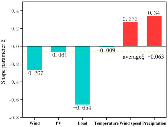
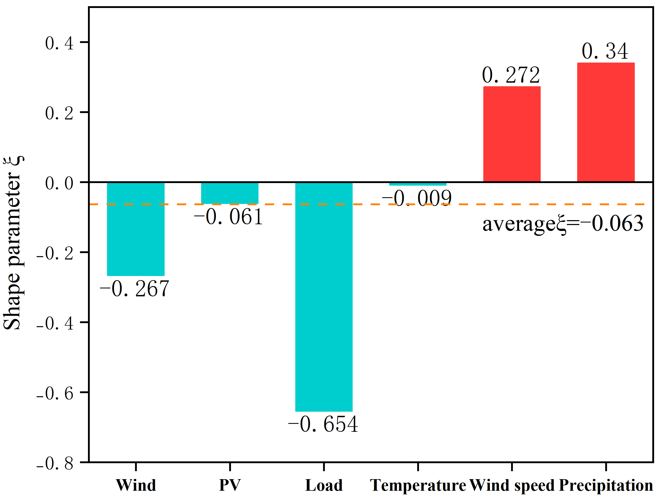
To evaluate the proposed extreme-event identification method, the tail characteristics of six key variables and the resulting extreme-event statistics are analyzed. Figure 1 shows the estimated GPD shape parameters. The ξ values of wind power, PV power, and load are negative, indicating that their extreme variations are constrained by physical operating limits. The ξ value of temperature is close to zero, suggesting an approximately exponential tail, whereas wind speed and precipitation exhibit positive ξ values, indicating heavier-tailed behavior. The average shape parameter is ξ = −0.063, suggesting an overall mildly bounded-tail characteristic, while the heavy tails of wind speed and precipitation indicate deviations from the light-tailed Gaussian assumption.

Figure 1. GPD shape parameters.

Table 2 summarizes the extreme events identified using the EVT-GPD and dual-path AND fusion strategy. Among 1460 daily samples, 177 days (12.1%) are classified as extreme events, with the remaining 1283 days identified as normal. Low-irradiance and high-wind events account for the largest proportions, with 82 days (5.6%) and 73 days (5.0%), respectively, whereas dust storms, snowstorms, and cold waves collectively account for only 1.5%. No heatwave events are identified during the study period. These results demonstrate the low-frequency and imbalanced nature of extreme events, particularly for rare hazards, providing a clear motivation for subsequent extreme-scenario augmentation.

Table 2. Statistics of identified extreme weather events.

Extreme Event Type	Days	Proportion
Cold Wave	4	0.3%
Snowstorm	8	0.5%
Dust Storm	10	0.7%
High Wind	73	5.0%
Heat Wave	0	0%
Low Irradiance	82	5.6%
Normal Weather	1283	87.9%
Total	1460	100%

3.3. Validation of Correlation-Preserving Probabilistic Modeling

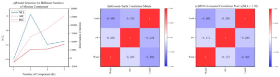
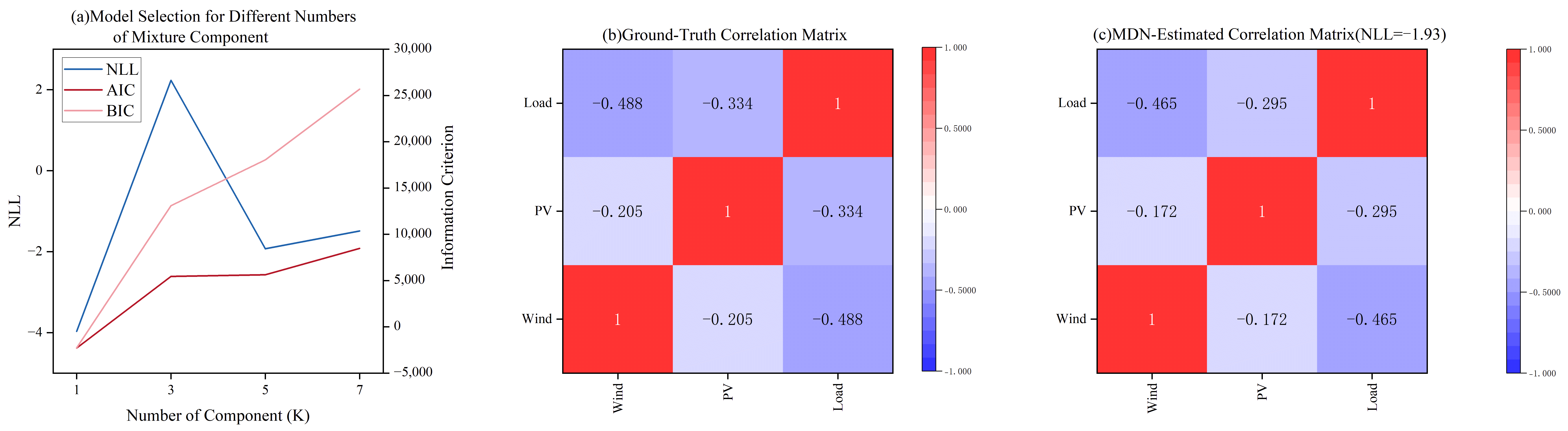
Since wind power, PV generation, and load are jointly influenced by meteorological conditions, their cross-variable dependencies should be explicitly considered in joint probabilistic modeling. Figure 2 presents the model selection and correlation reconstruction results of the proposed full-covariance MDN.

Figure 2. Mixture-component selection and correlation reconstruction of the proposed full-covariance MDN.

As shown in Figure 2a, the number of mixture components (K) is evaluated over a range of candidate values using the NLL, Akaike information criterion (AIC), and Bayesian information criterion (BIC). Increasing (K) initially improves the distributional fitting capability, whereas further increasing the number of components provides limited additional benefits relative to the increased model complexity. Considering the joint evidence from the likelihood-based and information-theoretic criteria, together with the need to maintain a compact and interpretable mixture representation, (K = 5) is selected for the subsequent experiments. In this evaluation, NLL is used to assess the probability-density fitting capability of the MDN, whereas AIC and BIC additionally account for model complexity. These criteria therefore provide complementary evidence for mixture-component selection rather than relying on correlation reconstruction alone.

Figure 2b presents the ground-truth correlation matrix calculated from the observed wind power, PV generation, and load data. Noticeable negative dependencies exist among all three variable pairs, with correlation coefficients of −0.205 for wind–PV, −0.488 for wind–load, and −0.334 for PV–load. These results demonstrate that the renewable generation and load variables exhibit significant cross-variable dependencies that cannot be adequately characterized by independent marginal distributions.

The correlation matrix estimated by the proposed full-covariance MDN is shown in Figure 2c. The estimated coefficients are −0.172, −0.465, and −0.295 for the wind–PV, wind–load, and PV–load pairs, respectively. Importantly, the MDN preserves both the signs and the relative magnitudes of the three observed correlations. The corresponding correlation reconstruction MAE is approximately 0.032, indicating a relatively small discrepancy between the estimated and ground-truth dependency structures. In particular, the strong negative wind–load correlation is retained, while the weaker wind–PV and PV–load dependencies are also reproduced with reasonable accuracy.

The correlation reconstruction results show that the full-covariance MDN can preserve the signs and relative magnitudes of the pairwise dependencies among wind power, PV generation, and load. However, correlation reconstruction evaluates pairwise dependency preservation and does not, by itself, constitute a complete validation of the multivariate probability density. Therefore, the MDN is evaluated using complementary criteria: NLL assesses probability-density fitting, AIC and BIC account for the trade-off between fitting performance and model complexity, and correlation reconstruction MAE evaluates the preservation of cross-variable dependencies. Taken together, these results provide a more comprehensive assessment of the joint-distribution modeling capability of the full-covariance MDN and support its use in the subsequent conditional scenario-generation stage.

3.4. Results of Physics-Constrained Scenario Generation

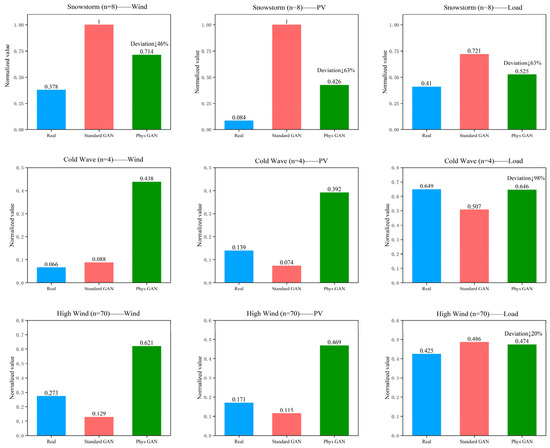
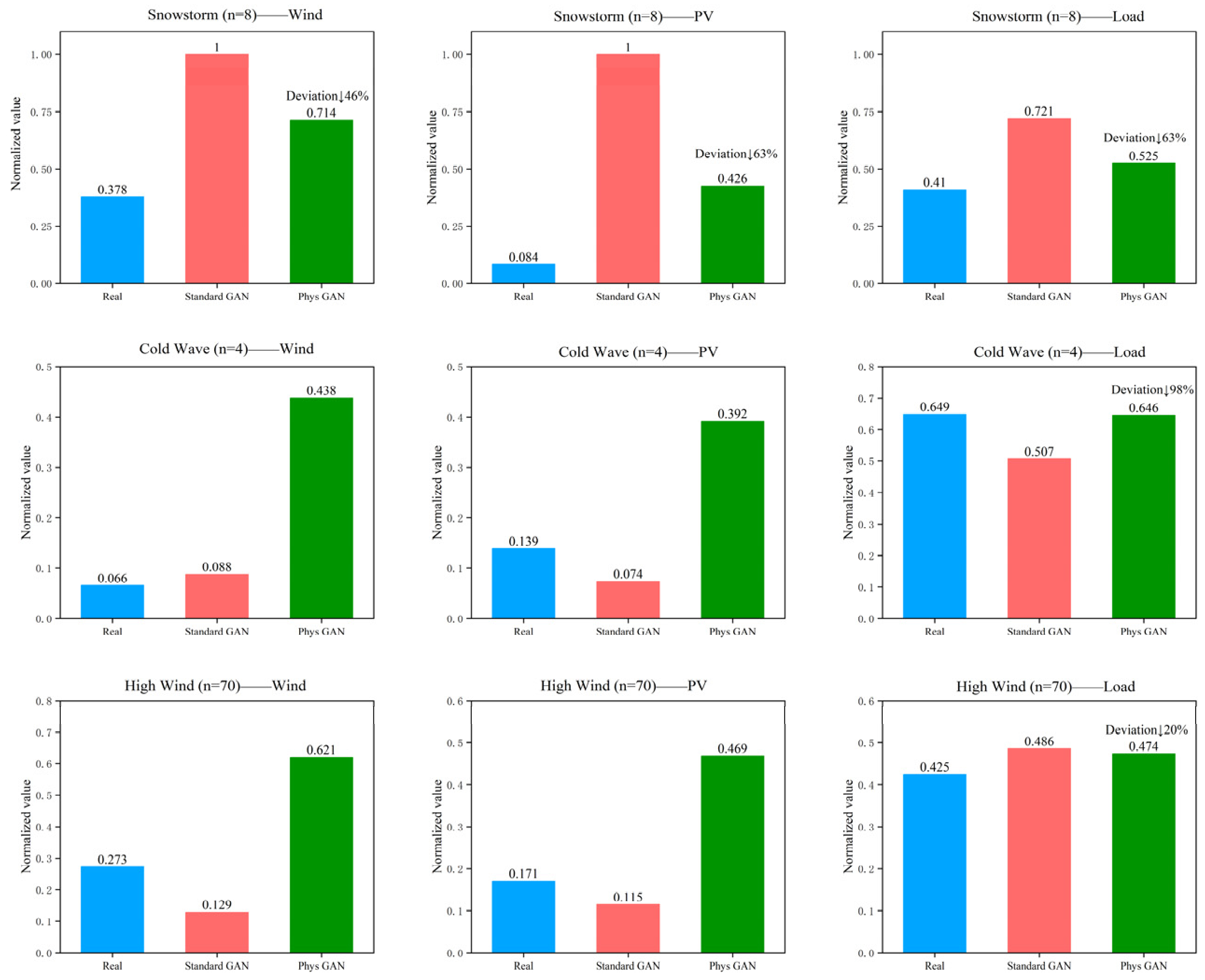
To evaluate the effectiveness of physical constraints in extreme-weather scenario generation, four WGAN-GP variants are compared, including the unconstrained model (A_Base), class-weighted model (B_Weight), fixed-constraint model (C_Fixed), and adaptive-boundary model (D_Adaptive). Figure 3 compares the statistical characteristics of generated and real extreme samples. The unconstrained model shows substantial deviations under low-frequency events. For example, under the snowstorm condition, the generated mean wind and PV powers of A_Base are both close to 1.000, whereas the corresponding real means are 0.378 and 0.084, respectively. After introducing fixed physical constraints, C_Fixed reduces these generated means to 0.714 and 0.426, with the corresponding deviations reduced by approximately 46% and 63%. Under the cold-wave condition, the generated mean load increases from 0.507 for A_Base to 0.646, approaching the real value of 0.649, while the mean bias decreases from 0.142 to 0.003. These results indicate that physical constraints can effectively improve the consistency between generated scenarios and actual extreme operating states, although their effects vary across variables and event types.

Figure 3. Comparison of statistical characteristics between real and generated extreme samples.

Table 3 further compares the four methods using the Wasserstein distance, maximum mean discrepancy (MMD), and mean bias. C_Fixed achieves the best overall performance, reducing the Wasserstein distance from 0.323 to 0.206, MMD from 1.210 to 0.887, and mean bias from 0.380 to 0.246, corresponding to reductions of approximately 36%, 27%, and 35%, respectively. B_Weight provides limited improvement in the overall distribution metrics but remains unstable for specific extreme events, with snowstorm PV bias and cold-wave load bias reaching 0.817 and 0.433, respectively. D_Adaptive obtains a Wasserstein distance of 0.228 and the lowest high-wind power bias of 0.200, but its MMD (1.083) and mean bias (0.289) remain higher than those of C_Fixed. This suggests that adaptive boundary estimation can be affected by the limited samples available for low-frequency extreme events, whereas fixed boundaries based on prior operational knowledge provide more stable physical guidance.

Table 3. Quantitative comparison of different WGAN-GP variants.

Variant	Wasserstein Distance	MMD	Mean Bias	PV Bias Under Snowstorm	Load Bias Under Cold Wave	Wind Bias Under High Wind
A_Base: Standard WGAN-GP	0.323	1.21	0.38	0.647	0.159	0.388
B_Weight: Class-Weighted WGAN-GP	0.286	1.158	0.376	0.817	0.433	0.338
C_Fixed: Fixed-Constraint WGAN-GP	0.206	0.887	0.246	0.342	0.003	0.347
D_Adaptive: Adaptive-Boundary WGAN-GP	0.228	1.083	0.289	0.373	0.344	0.200

Overall, the results demonstrate that combining distribution learning with physical operating constraints can improve both the statistical consistency and physical plausibility of generated extreme scenarios. In the present case, C_Fixed provides the most stable overall performance, indicating that physically interpretable prior constraints can be more reliable than data-driven adaptive boundaries under limited extreme samples. Therefore, C_Fixed is selected as the scenario augmentation strategy for subsequent LSTM probabilistic forecasting.

To evaluate temporal and cross-variable dependency preservation, lag-one autocorrelation and pairwise Pearson correlations were calculated on the TEST set. The generated wind, PV, and load trajectories achieved lag-one correlations of 0.9825, 0.9516, and 0.9231, close to the real values of 0.9923, 0.9910, and 0.9387, with a mean absolute error of 0.0216. For wind–PV, wind–load, and PV–load, the generated correlations were −0.4439, −0.0965, and −0.1933, compared with real values of −0.3561, −0.3581, and −0.0877, yielding an average error of 0.1516. Overall, the generated scenarios preserve temporal autocorrelation well, while cross-variable dependence is partially retained.

3.5. Probabilistic Forecasting Performance Analysis

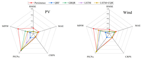
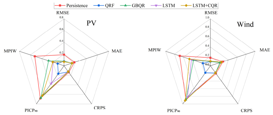
To evaluate the proposed probabilistic forecasting method, five approaches, including persistence, quantile random forest (QRF), gradient boosting quantile regression (GBQR), LSTM, and LSTM+CQR, are compared in terms of RMSE, CRPS, and PICP₉₀. As shown in Figure 4, LSTM achieves the lowest PV RMSE of 0.066, compared with 0.190 for Persistence, representing a reduction of approximately 65%. QRF and GBQR obtain RMSE values of 0.078 and 0.077, respectively. For wind power, the RMSE values of QRF, GBQR, and LSTM are 0.086, 0.088, and 0.095, respectively, indicating greater forecasting uncertainty than for PV power. In terms of probabilistic performance, LSTM achieves CRPS values of 0.012 and 0.021 for PV and wind power, respectively, while GBQR obtains 0.017 and 0.018. However, the original LSTM prediction intervals show insufficient coverage, with PICP₉₀ values of 0.450 for PV and 0.788 for wind power. After CQR calibration, the RMSE and CRPS remain unchanged, whereas PICP₉₀ increases to 0.895 and 0.893, respectively. For PV forecasting, this substantial improvement in coverage is achieved with only a small increase in MPIW from 0.143 to 0.152 (approximately 6.3%), while ACE for the nominal 90% prediction interval (ACE₉₀) decreases from 0.450 to 0.005. This indicates that CQR effectively corrects the severe undercoverage of the original PV intervals without excessive loss of interval sharpness. For wind-power forecasting, PICP₉₀ increases from 0.788 to 0.893 and ACE₉₀ decreases from 0.112 to 0.007, but MPIW increases from 0.308 to 0.361 (approximately 17.2%). Compared with PV, the improvement in wind-power coverage therefore requires a larger interval expansion, suggesting that wind-power uncertainty is more difficult to calibrate and exhibits stronger dispersion. Overall, CQR brings both PV and wind-power coverage close to the nominal 90% level, but the associated sharpness–coverage trade-off is more pronounced for wind power.

Figure 4. Comparison of point and probabilistic forecasting performance for PV and wind power.

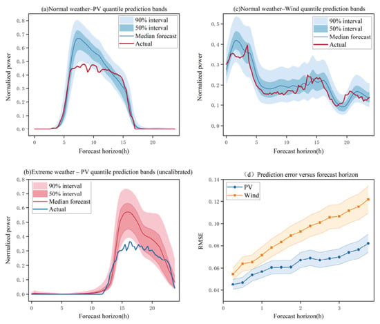
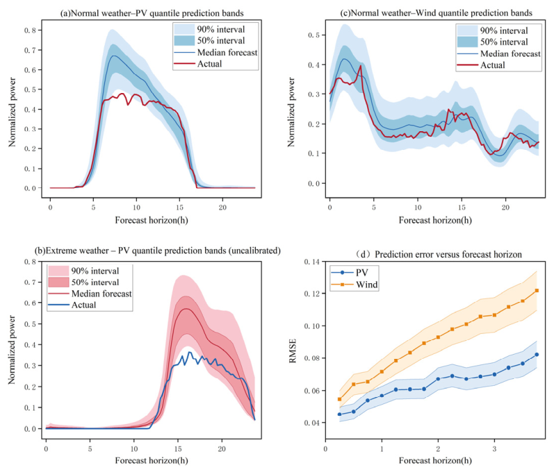
To further examine the temporal characteristics of the prediction intervals, Figure 5 presents representative probabilistic forecasts under normal and extreme weather conditions, together with the variation in forecasting errors over the forecast horizon. Under normal weather conditions, the predicted PV median closely follows the actual power profile and captures the main ramp-up and ramp-down processes. The prediction interval widens during periods of rapid power variation and narrows as the output approaches zero, indicating that the model adapts the interval width to time-varying uncertainty. Under extreme weather conditions, the PV prediction interval becomes substantially wider, but a systematic deviation remains between the predicted median and actual output. The PICP₉₀ further decreases from 0.450 over the overall test set to 0.204 under extreme weather, indicating that simply widening the prediction interval is insufficient to ensure reliable coverage. Wind power exhibits stronger stochastic fluctuations, with the predicted median generally following the observed variations but showing larger deviations during rapid changes, while the prediction interval dynamically varies with the uncertainty level.

Figure 5. Probabilistic forecasting intervals and forecasting errors under different weather conditions.

Figure 5d further shows that the forecasting errors of both PV and wind power increase with the forecast horizon. The PV RMSE increases from approximately 0.045 to 0.08, whereas the wind RMSE increases from approximately 0.055 to 0.12. Wind power consistently exhibits higher forecasting errors, and the gap between wind and PV gradually increases with the forecast horizon, indicating stronger uncertainty accumulation caused by the stochastic evolution of wind conditions. Overall, Figure 4 and Figure 5 demonstrate that LSTM effectively captures the temporal dependencies of wind and PV power and dynamically adjusts the prediction intervals according to forecast uncertainty, but evident interval miscalibration remains under extreme weather conditions. LSTM+CQR increases the overall PICP₉₀ to 0.895 for PV and 0.893 for wind power while maintaining essentially unchanged RMSE and CRPS, confirming its effectiveness in improving interval reliability. However, the coverage under extreme weather remains below the target 90%, motivating further analysis of CQR calibration performance under different weather conditions.

3.6. Uncertainty Calibration Analysis

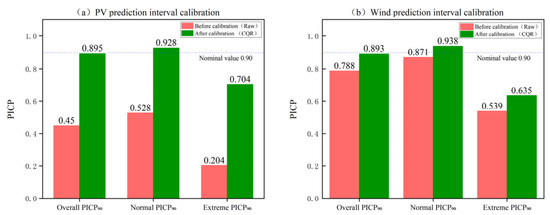
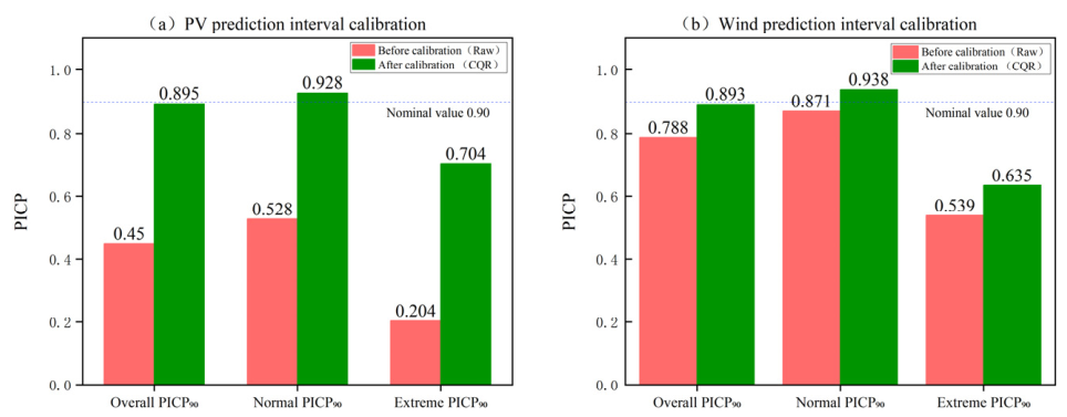
To evaluate the effectiveness of CQR in improving prediction-interval reliability under extreme weather conditions, Figure 6 compares the PICP₉₀ before and after calibration for PV and wind power forecasting. For PV forecasting, the uncalibrated model exhibits evident interval undercoverage, with an overall PICP₉₀ of only 0.450, compared with 0.528 under normal weather and 0.204 under extreme weather. After CQR calibration, the overall PICP₉₀ increases to 0.895, while the coverage under normal and extreme weather conditions increases to 0.928 and 0.704, respectively. These results demonstrate that CQR can effectively correct the coverage bias induced by extreme-weather distribution shifts. However, the extreme-weather PICP₉₀ remains below the target level of 0.90, indicating that post hoc calibration alone is insufficient to fully recover the error distribution when extreme samples are scarce, further highlighting the need for extreme-scenario augmentation.

Figure 6. PICP₉₀ calibration performance before and after CQR under different weather conditions.

Wind power exhibits higher interval coverage before calibration, with an overall PICP₉₀ of 0.788 and values of 0.871 and 0.539 under normal and extreme weather conditions, respectively. After CQR calibration, the overall PICP₉₀ increases to 0.893, reaching 0.938 under normal weather, whereas the extreme-weather coverage increases only to 0.635. This difference indicates distinct uncertainty characteristics between PV and wind power under extreme weather conditions. PV forecasting is more sensitive to irradiance variations, which can introduce systematic prediction biases during extreme events, resulting in a more pronounced improvement from CQR. In contrast, wind power forecasting is more strongly affected by stochastic wind-speed fluctuations and exhibits more complex error distributions, limiting the effectiveness of a single calibration strategy under extreme conditions.

3.7. Partial Ablation

To further examine the contributions of the extreme-weather-aware and uncertainty-calibration modules, a partial ablation analysis is conducted under extreme weather conditions. As shown in Table 4, removing the extreme-weather-aware module reduces the PV PICP₉₀ from 0.704 to 0.462, corresponding to a 34.3% decrease, indicating that explicit state identification improves the model’s ability to characterize extreme operating conditions. For wind power, the corresponding PICP₉₀ increases from 0.635 to 0.805, suggesting that coverage alone may be affected by interval width and should therefore be interpreted jointly with other probabilistic metrics. Removing CQR results in a substantial decrease in PICP₉₀, from 0.704 to 0.204 for PV and from 0.635 to 0.539 for wind power, demonstrating the importance of post hoc calibration for improving interval reliability. The contribution of physics-constrained scenario generation is instead evaluated through the scenario-quality analysis in Section 3.4 and the end-to-end augmentation experiment in Section 3.8.

Table 4. Ablation results of the proposed framework.

Experimental Configuration	PV RMSE	PV Extreme PICP90	Wind RMSE	Wind Extreme PICP90
Full framework	0.066	0.704	0.095	0.635
−Extreme-weather awareness	0.064	0.462	0.090	0.805
−CQR calibration	0.066	0.204	0.095	0.539

3.8. Equal-Compute Closed-Loop Validation of GAN-Augmented Training

To assess GAN-based augmentation under an equal computational budget, we compared three training configurations. Baseline used 122,562 original real TRAIN windows, including 12,350 extreme-weather windows. Extra-real added 700 real extreme-weather windows sampled with replacement exclusively from those 12,350 TRAIN windows; these were repeated training observations, not newly collected observations. GAN-Augmented added 700 generated extreme-weather windows, comprising 140 windows for each of five event classes: cold wave, snowstorm, sandstorm, high wind, and low radiation. The resulting training pools contained 122,562, 123,262, and 123,262 windows, respectively. No validation, CQR calibration, or final-evaluation window was resampled into Extra-real.

All three arms used the same LSTM architecture, batch size of 128, validation criterion, and CQR protocol. Each epoch used 958 mini-batch updates, or 122,624 sampled window positions, from the respective shuffled training pool. When a pool was exhausted, sampling continued from a new shuffled pass. Thus, Baseline required 62 repeated positions per epoch; each augmented pool supplied 122,624 of its 123,262 positions per epoch and was shuffled again in subsequent epochs. Over 100 epochs, each arm received 95,800 optimizer updates.

Under these controlled conditions, GAN augmentation improved forecasting performance on the extreme-weather subset. For PV forecasting, RMSE decreased from 0.0699 to 0.0567 and PICP₉₀ increased from 0.8933 to 0.9020. For wind-power forecasting, RMSE decreased from 0.0939 to 0.0823 and PICP₉₀ increased from 0.7341 to 0.8024, while ACE₉₀ decreased substantially from 0.1659 to 0.0976. These results indicate that GAN augmentation can improve forecasting performance when extreme-weather training samples are scarce, particularly in terms of predictive accuracy and interval reliability.

The Extra-real control further shows that the effects of real-sample and GAN-based augmentation are not identical. Although Extra-real achieved a slightly lower RMSE for extreme wind-power forecasting, GAN-Augmented provided better PICP₉₀ and ACE₉₀ for extreme wind power and stronger performance across several extreme-PV metrics. This comparison helps distinguish the effect of increasing the number of training samples from the additional contribution of GAN-generated extreme scenarios.

4. Discussion

4.1. Effectiveness of the Proposed Framework

The experimental results indicate that probabilistic forecasting under extreme weather is jointly affected by extreme-state scarcity, cross-variable dependence, and prediction-interval miscalibration. Among the 1460 historical days, only 177 are identified as extreme events, accounting for 12.1%, which limits the ability of conventional models to learn rare operating states. The ablation results further show that removing extreme-weather awareness reduces the extreme-weather PICP₉₀ of PV forecasting from 0.704 to 0.462. In addition, the full-covariance MDN achieves a correlation reconstruction MAE of 0.032, indicating that the main dependency structure among wind power, PV generation, and load can be represented with relatively small pairwise-correlation discrepancies.

The scenario-generation results further show that distributional consistency alone is insufficient for evaluating multi-step extreme scenarios. In addition to the distributional metrics reported in Section 3.4, trajectory-level validation shows that the lag-one correlations of the generated wind, PV, and load sequences are 0.9825, 0.9516, and 0.9231, respectively, compared with 0.9923, 0.9910, and 0.9387 in the real data. The resulting lag-one correlation MAE of 0.0216 indicates strong preservation of short-term temporal dependence. Cross-variable dependence is preserved less uniformly, with a pairwise-correlation MAE of 0.1516, indicating that reproducing the full strength of inter-variable dependence remains more challenging than preserving temporal continuity.

The controlled downstream experiment further demonstrates the practical value of scenario augmentation under the same computational budget. GAN-augmented training reduces the extreme-weather PV RMSE from 0.0699 to 0.0567 and the wind-power RMSE from 0.0939 to 0.0823. The corresponding PICP₉₀ values increase from 0.8933 to 0.9020 for PV and from 0.7341 to 0.8024 for wind power, while wind-power ACE₉₀ decreases from 0.1659 to 0.0976. Together, these results support the role of the identification–modeling–generation–forecasting–calibration chain, while also showing that temporal consistency and cross-variable dependency preservation should be evaluated separately.

4.2. Complementary Roles of Scenario Augmentation and Calibration

Scenario augmentation and uncertainty calibration address different stages of the forecasting process. WGAN-GP enriches the training data by increasing the representation of rare extreme states, whereas CQR adjusts the reliability of the prediction intervals after forecasting. The experimental results confirm this distinction. For extreme PV forecasting, PICP₉₀ increases from 0.204 to 0.704 after CQR calibration. In contrast, the controlled augmentation experiment modifies the training distribution itself: GAN-augmented training reduces extreme-weather PV RMSE from 0.0699 to 0.0567 and increases PICP₉₀ from 0.8933 to 0.9020. These results should not be interpreted as a single sequential numerical improvement because the calibration and augmentation experiments evaluate different stages of the forecasting pipeline. Rather, they demonstrate that scenario augmentation primarily affects what the forecasting model learns from rare operating states, whereas CQR acts after model training to correct interval coverage.

The two mechanisms also show different effectiveness for wind and PV forecasting. Although CQR substantially improves wind-power coverage under normal conditions, the extreme-weather PICP₉₀ increases only from 0.539 to 0.635, indicating that extreme wind-power errors exhibit more complex stochastic characteristics that cannot be fully corrected by a unified post hoc calibration strategy. In the controlled augmentation experiment, GAN-generated samples improve extreme-wind PICP90 from 0.7341 to 0.8024 and reduce ACE90 from 0.1659 to 0.0976, indicating that enriching the training distribution can address a different component of the uncertainty problem. Therefore, scenario augmentation and interval calibration should be considered complementary rather than alternative strategies, while further state-dependent calibration may still be required for rare extreme conditions.

4.3. Practical Implications and Limitations

From an operational perspective, the proposed framework provides probabilistic information that can support risk-aware operation under extreme weather. Compared with deterministic forecasts, calibrated prediction intervals can better indicate potential deviations in renewable generation and therefore provide useful information for reserve allocation, energy-storage scheduling, and risk-constrained operation. The joint modeling of wind power, PV generation, and load further enables the forecasting system to capture their coordinated uncertainty rather than treating each variable independently.

From a computational perspective, the MDN and WGAN-GP are mainly employed in the offline stage for joint-distribution modeling and extreme-scenario augmentation. During online operation, only the trained LSTM is required for forward forecasting, followed by CQR-based interval calibration using the previously estimated correction parameters. Therefore, the online computational burden is substantially lower than that of the offline training stage, supporting the potential use of the framework in rolling operational forecasting. The exact inference latency depends on the hardware and deployment environment and should be evaluated in future real-time implementations.

Several limitations should nevertheless be noted. The number of extreme-weather samples is still limited, which may restrict generalization to rare or unseen extreme events. Further validation using larger multi-region datasets would therefore be valuable.

5. Conclusions

This paper proposes a unified framework for probabilistic forecasting of wind and PV power under extreme weather, addressing the challenges of extreme-sample scarcity, enhanced wind–PV–load dependency, and prediction-interval miscalibration. Using 1460 days of wind power, PV power, load, and meteorological data from the Hai xi region of Qinghai Province during 2021–2024, the effectiveness of the proposed framework is systematically evaluated.

The EVT-GPD and dual-path AND strategy identifies 177 extreme-event days, accounting for 12.1% of the dataset, confirming the low-frequency and imbalanced characteristics of extreme operating states. The full-covariance MDN effectively captures the joint dependencies among wind power, PV power, and load, achieving a correlation reconstruction MAE of 0.032. For multi-step scenario generation, the physics-constrained WGAN-GP produces wind, PV, and load trajectories with a lag-one correlation MAE of 0.0216, demonstrating strong preservation of short-term temporal dependence. The pairwise cross-variable correlation MAE is 0.1516, showing that the main signs of the observed dependencies are retained but that their magnitudes are only partially reproduced.

The LSTM+CQR model substantially improves prediction-interval reliability while maintaining forecasting performance. The overall PICP₉₀ reaches 0.895 for PV and 0.893 for wind power, while under extreme weather it increases from 0.204 to 0.704 for PV and from 0.539 to 0.635 for wind power. Under an equal computational budget, GAN-augmented training further reduces extreme-weather PV RMSE from 0.0699 to 0.0567 and wind-power RMSE from 0.0939 to 0.0823. The corresponding PICP₉₀ values increase from 0.8933 to 0.9020 for PV and from 0.7341 to 0.8024 for wind power, with wind-power ACE₉₀ decreasing from 0.1659 to 0.0976.

Overall, the results demonstrate that reliable probabilistic forecasting under extreme weather requires the joint consideration of state heterogeneity, extreme-sample scarcity, cross-variable dependencies, and interval miscalibration. The proposed framework establishes a complete closed loop from extreme-state identification and dependency-preserving probabilistic modeling to physics-constrained scenario augmentation and calibrated probabilistic forecasting. The remaining discrepancies in cross-variable correlation and the limited number of rare extreme events indicate that further improvements are still required. Future work will focus on enlarging extreme-event datasets, incorporating additional meteorological and power-system constraints, and developing state-conditional dynamic calibration strategies to improve generalization to rare and unseen extreme events.

References

- Hong, T.; Pinson, P.; Wang, Y.; Weron, R.; Yang, D.; Zareipour, H. Energy forecasting: A review and outlook. IEEE Open Access J. Power Energy 2020, 7, 376–388. [Google Scholar] [CrossRef] [Scilit]
- van der Meer, D.; Widén, J.; Munkhammar, J. Review on probabilistic forecasting of photovoltaic power production and electricity consumption. Renew. Sustain. Energy Rev. 2017, 81, 1484–1512. [Google Scholar] [CrossRef] [Scilit]
- Panteli, M.; Mancarella, P. Influence of extreme weather and climate change on the resilience of power systems: Impacts and possible mitigation strategies. Electr. Power Syst. Res. 2015, 127, 259–270. [Google Scholar] [CrossRef] [Scilit]
- Pinson, P. Wind energy: Forecasting challenges for its operational management. Stat. Sci. 2013, 28, 564–585. [Google Scholar] [CrossRef] [Scilit]
- Foley, A.M.; Leahy, P.G.; Marvuglia, A.; Mckeogh, E.J. Current methods and advances in forecasting of wind power generation. Renew. Energy 2012, 37, 1–8. [Google Scholar] [CrossRef] [Scilit]
- Wang, H.; Lei, Z.; Zhang, X.; Zhou, B.; Peng, J. A review of deep learning for renewable energy forecasting. Energy Convers. Manag. 2019, 198, 111799. [Google Scholar] [CrossRef] [Scilit]
- Hong, T.; Fan, S. Probabilistic electric load forecasting: A tutorial review. Int. J. Forecast. 2016, 32, 914–938. [Google Scholar] [CrossRef] [Scilit]
- Gneiting, T.; Katzfuss, M. Probabilistic forecasting. Annu. Rev. Stat. Appl. 2014, 1, 125–151. [Google Scholar] [CrossRef] [Scilit]
- Panteli, M.; Mancarella, P. The grid: Stronger, bigger, smarter? Presenting a conceptual framework of power system resilience. In Proceedings of 2015 IEEE Power & Energy Society General Meeting (PESGM 2015), Denver, CO, USA, 26–30 July 2015; IEEE: New York, NY, USA, 2015; pp. 58–66. [Google Scholar]
- Angelopoulos, A.N.; Bates, S. A gentle introduction to conformal prediction and distribution-free uncertainty quantification. arXiv 2021, arXiv:2107.07511. [Google Scholar] [CrossRef] [Scilit]
- Kuleshov, V.; Fenner, N.; Ermon, S. Accurate uncertainties for deep learning using calibrated regression. In Proceedings of the 35th International Conference on Machine Learning (ICML 2018), Stockholm, Sweden, 10 July–15 November 2026; pp. 2796–2804. [Google Scholar]
- Coles, S. An Introduction to Statistical Modeling of Extreme Values. J. Am. Stat. Assoc. 2002, 97, 1204. [Google Scholar] [CrossRef] [Scilit]
- Pickands, J. Statistical inference using extreme order statistics. Ann. Stat. 1975, 3, 119–131. [Google Scholar] [CrossRef] [Scilit]
- Panteli, M.; Mancarella, P. Modeling and evaluating the resilience of critical electrical power infrastructure to extreme weather events. IEEE Syst. J. 2017, 11, 1733–1742. [Google Scholar] [CrossRef] [Scilit]
- Zhang, H.; Liu, Y.; Yan, J.; Han, S.; Li, L.; Long, Q. Improved deep mixture density network for regional wind power probabilistic forecasting. IEEE Trans. Power Syst. 2020, 35, 2549–2560. [Google Scholar] [CrossRef] [Scilit]
- Men, Z.; Yee, E.; Lien, F.; Wen, D.; Chen, Y. Short-term wind speed and power forecasting using an ensemble of mixture density neural networks. Renew. Energy 2016, 87, 203–211. [Google Scholar] [CrossRef] [Scilit]
- Eikeland, O.F.; Hovem, F.D.; Olsen, T.E.; Chiesa, M.; Bianchi, F.M. Probabilistic forecasts of wind power generation in regions with complex topography using deep learning methods: An Arctic case. Energy Convers. Manag. X 2022, 15, 100239. [Google Scholar] [CrossRef] [Scilit]
- Bessa, R.J.; Trindade, A.; Silva, C.S.P.; Miranda, V. Probabilistic solar power forecasting in smart grids using distributed information. Int. J. Electr. Power Energy Syst. 2015, 72, 16–23. [Google Scholar] [CrossRef] [Scilit]
- Zhang, G. Renewable Scenario Generation Based on Improved Conditional Generative Adversarial Networks. In Proceedings of 2025 4th International Symposium on New Energy Technology Innovation and Low Carbon Development (NET-LC 2025), Hangzhou, China, 9–11 May 2025; IEEE: New York, NY, USA, 2025; pp. 58–66. [Google Scholar]
- Gulrajani, I.; Ahmed, F.; Arjovsky, M.; Dumoulin, V.; Courville, A.C. Improved training of Wasserstein GANs. In Proceedings of 2017 Neural Information Processing Systems (NeurIPS 2017), Los Angeles, CA, USA, 4–9 December 2017; Curran Associates Inc.: Red Hook, NY, USA, 2017; pp. 5767–5777. [Google Scholar]
- Schmidhuber, J.; Hochreiter, S. Long short-term memory. Neural Comput. 1997, 9, 1735–1780. [Google Scholar] [CrossRef] [Scilit] [PubMed]
- Salinas, D.; Flunkert, V.; Gasthaus, J.; Januschowski, T. DeepAR: Probabilistic forecasting with autoregressive recurrent networks. Int. J. Forecast. 2020, 36, 1181–1191. [Google Scholar] [CrossRef] [Scilit]
- Koenker, R.; Hallock, K.F. Quantile regression. J. Econ. Perspect. 2001, 15, 143–156. [Google Scholar] [CrossRef] [Scilit]
- Vovk, V.; Gammerman, A.; Shafer, G. On-line compression modeling I: Conformal prediction. In Algorithmic Learning in a Random World; Springer: New York, NY, USA; Boston, MA, USA, 2005; pp. 189–221. [Google Scholar]
- Romano, Y.; Patterson, E.; Candes, E. Conformalized quantile regression. In Proceedings of 2019 Neural Information Processing Systems (NeurIPS 2019), Vancouver, BC, Canada; Curran Associates Inc.: Red Hook, NY, USA, 2019; pp. 3543–3553. [Google Scholar]
- Lauret, P.; David, M.; Pedro, H.T.C. Probabilistic solar forecasting using quantile regression models. Energies 2017, 10, 1591. [Google Scholar] [CrossRef] [Scilit]
- Raissi, M.; Perdikaris, P.; Karniadakis, G.E. Physics-informed neural networks: A deep learning framework for solving forward and inverse problems involving nonlinear PDEs. J. Comput. Phys. 2019, 378, 686–707. [Google Scholar] [CrossRef] [Scilit]
- Karniadakis, G.E.; Kevrekidis, I.G.; Lu, L.; Perdikaris, P.; Wang, S.; Yang, L. Physics-informed machine learning. Nat. Rev. Phys. 2021, 3, 422–440. [Google Scholar] [CrossRef] [Scilit]
- Nowotarski, J.; Weron, R. Computing electricity price prediction intervals using quantile regression and forecast averaging. Comput. Stat. 2015, 30, 791–803. [Google Scholar] [CrossRef] [Scilit]
- Ren, X.; Liu, Y.; Zhang, F.; Li, L. A deep learning quantile regression photovoltaic power-forecasting method under a priori knowledge injection. Energies 2024, 17, 4026. [Google Scholar] [CrossRef] [Scilit]
- Wang, G.; Zhou, Y.; Yan, Y.; Zhou, Z.; Yang, Z.; Dai, L.; Huang, J. Probabilistic photovoltaic power forecasting with reliable uncertainty quantification via multi-scale temporal-spatial attention and conformalized quantile regression. Sustainability 2026, 18, 739. [Google Scholar] [CrossRef] [Scilit]
- Gneiting, T.; Raftery, A.E. Strictly proper scoring rules, prediction, and estimation. J. Am. Stat. Assoc. 2007, 102, 359–378. [Google Scholar] [CrossRef] [Scilit]
Disclaimer/Publisher’s Note: The statements, opinions and data contained in all publications are solely those of the individual author(s) and contributor(s) and not of MDPI and/or the editor(s). MDPI and/or the editor(s) disclaim responsibility for any injury to people or property resulting from any ideas, methods, instructions or products referred to in the content. |
© 2026 by the authors. Licensee MDPI, Basel, Switzerland. This article is an open access article distributed under the terms and conditions of the Creative Commons Attribution (CC BY) license.