Evaluation of Corrosion Progression in X210Cr12 Tool Steel in a Marine-like Chloride Environment Using SEM/EDS and PCA Techniques

Abstract

Corrosion of high-chromium tool steels in marine environments is a major concern for structural materials, as chloride-rich conditions accelerate material degradation and reduce service life. The corrosion process involves complex interactions among passive film degradation, localized pitting, and surface defect evolution. This study investigates the corrosion progression of X210Cr12 tool steel immersed in a 3.5 wt.% NaCl solution, representing a marine-like chloride environment. Corrosion progression was monitored by combining mass loss measurements, SEM/EDS characterization, quantitative image analysis, and principal component analysis (PCA). The results reveal three distinct stages of surface degradation: initial pit nucleation, pit propagation accompanied by formation of new defects and growth of already existing ones, and pit coalescence with accelerated mass loss after 90 days of exposure, which can be associated with pronounced chromium depletion and degradation of the protective surface layer. The cumulative mass loss increased from 0.024 g after 30 days to 0.153 g after 120 days, while the calculated corrosion rate increased from 0.067 to 0.107 mm/year. Image analysis showed an increase in the degraded surface area from 0.089% to 13.34% at 120 days. EDS measurements indicated a pronounced decrease in surface chromium content accompanied by increasing oxygen content in corroded regions. PCA identified the most informative morphological descriptors, showing that size-related parameters dominated in the early stages of corrosion, while shape-related descriptors became more important during advanced stages of degradation. The proposed methodology provides a data-driven approach for monitoring corrosion progression and identifying morphological parameters associated with different stages of surface degradation under marine-like chloride conditions.

1. Introduction

Corrosion refers to the gradual deterioration of a material due to chemical or electrochemical reactions with its environment, particularly in aggressive marine conditions where seawater acts as a complex electrolyte promoting pitting, crevice corrosion, and biofouling-enhanced degradation. Seawater, containing 3.5–4% salts (primarily NaCl, ~86%) along with Mg²⁺, Ca²⁺, and K⁺ ions, forms strong alkalis, while SO₄²⁻ and HCO₃⁻ produce weak acids at pH ~8. Such an environment drives heterogeneous corrosion through chemical, physical (flow/temperature), and biological mechanisms. Unlike simplified 3.5% NaCl simulants, natural seawater contains dissolved O₂/CO₂, organic matter, and microbes, amplifying variability, with Setchenow constants confirming close electrochemical similarity yet reflecting real-world complexity [1,2,3,4]. Seawater is one of the most aggressive fluids for steels commonly used in marine engineering. Extensive research has therefore focused on their corrosion behavior, primarily through electrochemical investigations [2,3,4,5,6,7], as well as monitoring corrosion-fatigue damage [8] and assessing internal defects in marine structures [9]. Its complex composition, including salts, dissolved gases, suspended solids, organic matter, and microorganisms [3,10,11,12], makes it challenging to isolate individual effects, so laboratory tests often employ simplified NaCl solutions for reproducibility [13,14,15].

X210Cr12 tool steel (1.45–1.70% C, 11.00–13.00% Cr, martensitic/ledeburitic) is widely utilized in marine engineering applications due to its superior hardness (62–64 HRC post-quenching/tempering), wear resistance against sediments and biofouling growth, minimal distortion during heat treatment, and ease of machining using Electrical Discharge Machining (EDM) for complex geometries [16]. Key applications of X210Cr12 include shipbuilding (propeller blades, stern tube bushings, anchor chain cutters, pipe fittings), subsea oil/gas infrastructure (pipeline repair clamps, remotely operated vehicle ROV manipulator tools, valve trims), offshore platforms (drilling dies, mud pump liners, caisson cutters), power plant seawater cooling systems (impellers, strainers), and underwater hardware exposed to tidal or alternate immersion conditions. The carbide-rich microstructure of this tool steel (M₇C₃, M₂₃C₆ primary carbides embedded in a martensitic matrix) provides abrasion resistance but makes it vulnerable to localized corrosion attack under prolonged exposure to seawater [16,17,18,19].

Despite its advantages, X210Cr12 faces severe corrosion risks in marine environments: chloride ions (Cl⁻) attack and thus can break the chromium/iron oxide passive layers at the carbide–matrix interfaces, initiating pitting (>10³ pits/cm² after 120 days according to ISO 11130:2017 alternate immersion in 3.5% NaCl) [20]. This pitting can evolve into undercutting and crevice corrosion, rapidly reducing its service life from years to months if untreated. The heterogeneous microstructure enhances galvanic coupling, while physical factors contribute to the erosion of protective films. Additionally, biofouling generates oxygen concentration cells, further accelerating degradation. Studies on AISI D3/X210Cr12 steels have shown that treatments such as deep cryogenic processing can significantly alter the corrosion resistance, with DCT samples exhibiting pitting and accelerated degradation due to microstructural changes [17,18,19]. Additionally, deep-sea analogs demonstrate accelerated corrosion kinetics in high-strength steels under increased pressure.

Previous studies regarding the corrosion of X210Cr12 tool steel have primarily focused on its electrochemical behavior in chloride environments. Uygur et al. [17] demonstrated, using electrochemical impedance spectroscopy and polarization, that untreated samples exhibit the highest corrosion resistance, whereas heat-treated and deep cryogenic treatment (DCT) samples develop significant pitting due to carbide refinement and chromium depletion. Similarly, Amini et al. [18] reported a 54% reduction in corrosion resistance following DCT, attributed to Cr loss and the increased density of martensite/carbonitride boundaries, which act as preferential corrosion sites. In contrast, Jovičević-Klug et al. [19] observed a 55–65% improvement in the corrosion resistance of X210Cr12 in Adriatic seawater compared to AISI 52100, which was attributed to the formation of corrosion products such as akaganeite and magnetite. Coating strategies have also proven effective: vanadium carbide (VC) layers applied via thermo-reactive deposition significantly enhanced corrosion resistance [21], titanium–tungsten nitride (Ti-W-N) coatings provided additional protection [22], and hafnium carbonitride (HfCN) coatings reduced the corrosion rate by 98% in 3.5% NaCl solutions [23].

However, critical gaps persist in the literature. Most studies report electrochemical data, SEM/EDS images, and mass loss results in isolation, without statistically integrating these datasets. Recent data-driven approaches have further demonstrated the potential of combining corrosion-related measurements with statistical and computational methods to improve corrosion prediction and support the interpretation of complex degradation datasets [24,25,26]. Data-driven and machine-learning approaches have increasingly been explored for corrosion risk assessment and prediction, highlighting the potential of multivariate analysis for extracting useful information from complex corrosion datasets [27,28]. Recent studies have also demonstrated the potential of automated image-based and machine-learning approaches for detecting and characterizing hidden corrosion damage, further supporting the use of quantitative image analysis for corrosion assessment [29]. Moreover, the role of carbide distribution versus matrix chromium content as the primary driver of pitting corrosion remains unclear, and no studies have comprehensively tracked the evolution of pitting damage over time. Long-term exposure to chloride-containing environments can progressively deteriorate the protective behavior of high-chromium steels and coatings, promoting localized corrosion and surface degradation [20,27]. The corrosion behavior of high-chromium steels is strongly dependent on the composition and physicochemical characteristics of chloride-containing environments [30,31].

This work addresses these gaps by employing a novel approach that integrates SEM/EDS analysis with quantitative image analysis and principal component analysis (PCA) to investigate X210Cr12 steel after 120 days of immersion in 3.5% NaCl. This multi-method approach provides a synergistic framework that combines chemical changes (such as chromium loss), morphological parameters (pit depth, area, density, aspect ratios), and statistical analysis to enhance the predictive accuracy of corrosion mechanisms.

The applied methodology offers a robust understanding of the corrosion process by revealing the hierarchical importance of different microstructural variables, aligning more closely with real-world failure mechanisms and contributing to a better understanding of corrosion progression under marine-like chloride conditions.

2. Materials and Methods

2.1. Material and Sample Preparation

This study examined X210Cr12 (AISI D3) tool steel, which is commonly produced by manufacturers worldwide and used in industries such as shipbuilding, oil and gas, and power plants. This steel is known for its high hardness and excellent wear resistance, although it exhibits limited toughness. Due to its high chromium content, X210Cr12 steel can form a protective Cr-passive film, providing a certain degree of corrosion resistance in chloride-containing environments. This characteristic enhances its relevance for applications in marine-like conditions, in addition to its high hardness and wear resistance.

The analyzed steel was high-carbon, high-chromium martensitic tool steel X210Cr12, produced by conventional casting and supplied in the as-cast condition. After casting, the material was shaped into beams and then hot-rolled. The beams were heated to 1024 °C, approximately two-thirds of iron’s melting temperature, before being processed through four flat rollers. The hot-rolled bars, supplied by SIJ Metal Ravne d.o.o., had dimensions of 30.8 × 3000 mm. For corrosion testing, cuboid sections with dimensions of 20 × 20 × 4 mm were cut from the steel bars and mechanically processed to obtain suitable dimensions. Prior to corrosion testing, the samples were mechanically ground and polished to obtain a uniform surface finish. For each measurement period, before mass loss determination and SEM analysis, the samples were ultrasonically cleaned in ethanol for 10 min, rinsed with distilled water, and dried under a stream of warm air to remove surface contamination. The chemical composition of the steel was determined through quantitative chemical analysis. Optical emission spectrometry (OES) was used for the elemental analysis of solid metallic samples, utilizing the Spectro MAXx-M LMM04 optical emission spectrometer. The results are shown in Table 1.

Table 1. Chemical composition of X210Cr12 tool steel (weight%).

Element (wt.%)	C	Cr	Mo	Mn	Si	Ni	Cu	Al	S	P
	2.09	11.16	0.03	0.28	0.22	0.11	0.03	0.012	0.006	0.016

The chemical composition indicates a high carbon content (2.09 wt.%) and significant chromium content (11.16 wt.%). Although chromium can promote the formation of a protective passive film and enhance corrosion resistance, the high carbon content can induce the formation of chromium carbides, which are responsible for the exceptional wear resistance and high hardness of this tool steel, but can locally reduce the chromium content in the matrix. As a result, the effective corrosion resistance of the steel in chloride-containing environments may be reduced, increasing its susceptibility to localized corrosion. Additionally, the steel contains only minor amounts of alloying elements such as molybdenum, manganese, and silicon, along with trace levels of nickel, copper, and aluminum, which limit further enhancement of corrosion resistance.

2.2. Corrosion Testing

Corrosion tests were performed by immersing samples in a 3.5 wt.% NaCl aqueous solution at 20 °C, in accordance with the following standards [13,14,15]. These tests represent a marine-like chloride environment to assess the material’s resistance to chloride-induced corrosion, which is relevant for marine-like and offshore applications. The corrosion testing procedures were based on standardized methodologies that provide consistent protocols and emphasize key principles for evaluating corrosion in saline environments. Corrosion monitoring was performed at intervals of 30, 60, 90, and 120 days of immersion in the solution. Weight loss measurements were taken, since this approach is crucial for evaluating corrosion in marine environments and quantifying material degradation under chloride exposure. The mass of the samples was measured before and after each immersion period using an analytical balance with an accuracy of ±0.1 mg. This method provided a direct assessment of material degradation, typically expressed as a corrosion rate (mm/year). Three independent specimens were prepared and exposed to each immersion period (30, 60, 90, and 120 days). Mass loss measurements, corrosion rate calculations and image-analysis results represent the mean values obtained from these three independent specimens. The corresponding standard deviations are reported in the Supplementary Material (SM).

2.2.1. Mass Loss Measurements and Corrosion Rate Calculation

One of the criteria used to evaluate the results of the corrosion test, in which the samples were immersed in a salt solution, is mass loss [32], determined by weighing the sample before and after exposure to the corrosive marine-like environment. After NaCl exposure, the samples were rinsed with distilled water and ethanol for five minutes to remove loosely adherent salts and surface debris. The samples were then dried and weighed. Chemical or electrolytic cleaning for complete removal of corrosion products was intentionally not applied. The decision was made because the objective of the study was to characterize surface changes and the formation and evolution of corrosion products during immersion by SEM. Therefore, the reported mass change represents the change in specimen mass after removal of loosely adherent deposits, while the adherent corrosion products were retained on the surface. The same cleaning and preparation procedure was used for the SEM observations [14,33]. After cleaning and weighing, the cumulative weight loss was calculated using Equation (1).

Mass loss (W) = W_initial − W_final

(1)

where W_initial and W_final are the masses (in grams) of the sample before and after corrosion experiments, respectively.

Another way to present material degradation is through the corrosion rate, which indicates the penetration depth of corrosion per unit time. This parameter was calculated from cumulative mass loss data, the exposed surface area of the sample (excluding any unexposed areas), and the density of the steel, according to Equation (2).

$$CR={\displaystyle \frac{K·W}{A·T·D}}$$

(2)

In this equation, CR is the corrosion rate in mm/year, K is a unit conversion constant equal to 87.6, T is the exposure time in hours, A is the exposed surface area in cm², W is the mass loss in milligrams, and D is the steel density in g/cm³ (7.7 g/cm³ in this study). The resulting value represents an average mass-loss-based corrosion rate over the exposed surface and exposure period. It is used here as a comparative indicator of overall material loss rather than as a measure of local pit penetration.

2.2.2. SEM/EDS Analysis

The surface morphology and elemental composition of the samples were analyzed at the beginning of the test and throughout the testing period to detect any changes that occurred. A field emission scanning electron microscope (FESEM, JEOL JSM 7001F, JEOL Ltd., Tokyo, Japan) was used for this analysis, along with energy-dispersive X-ray spectroscopy (EDS) using the OXFORD Xplore 15 instrument. The results of these tests provided detailed information that enabled the identification and discussion of corrosion mechanisms and the susceptibility of the steel to localized attack in chloride-containing environments.

2.2.3. Image Analysis

In addition to assessing mass loss, the degradation of the sample’s surface was monitored using SEM images and image analysis performed with the Image Pro Plus program. Image analysis is a valuable tool for quantifying sample degradation and morphology using various morphological parameters, which are described in detail in numerous studies [32,34,35]. The corrosion-induced damages on the sample’s surface were evaluated through image analysis of SEM micrographs by Image-Pro Plus 6.0 (IPP) software package (Media Cybernetics, 2006, Rockville, MD, USA). This software enables the quantification of various descriptors, facilitating a morphological characterization of the resulting defects. In this study, specific morphological descriptors were selected for analysis. Quantitative analysis of the SEM images was performed for each exposure period; three SEM micrographs were analyzed for each of three independent specimens. The micrographs were acquired at the same magnification. Image segmentation was performed using the automatic thresholding function of the software to distinguish the degraded/damaged regions from the remaining surface. The same thresholding approach and image-acquisition conditions were used for all analyzed images. The analyzed field of view was approximately 1,117,577 µm² (approximately 1215.774 × 919.231 µm). The obtained measurements were averaged across the replicate images/specimens for each exposure period. The representative area for analysis, and it was calculated as P₀ = 1,117,577 µm² by measuring the area of the photo using the measurement bar.

No additional image preprocessing (filtering, contrast enhancement, etc.) was applied beyond the automatic thresholding function of Image-Pro Plus 6.0, in order to minimize operator-dependent variability. The same thresholding settings and analysis protocol were applied consistently to all micrographs. The mean values obtained from the nine micrographs (3 specimens × 3 images) per exposure period were used for the reported results.

The selected morphological parameters were chosen based on their sensitivity to various stages of pit evolution during corrosion. Parameters related to the size of defects, such as Area, Diameters_{maximum/minimum/mean}, and Radius_{maximum/minimum}, were selected because they quantitatively reflect the overall growth and expansion of corrosion defects, enabling the monitoring of pit propagation over time. Parameters related to the shape of defects, including Roundness, Radius Ratio, and Perimeter Ratios, were selected for their ability to effectively highlight deviations from ideal circular geometry. Together, these parameters provided insights into the morphology of corrosion defects across different stages, assessing both the extent and the geometry of the pits. Additionally, the selection of specific parameters was further guided by prior authors’ experience and studies [26,36,37,38], which demonstrated their reliability and sensitivity in characterizing corrosion-related surface features.

• Area: the measured surface enclosed by each detected feature, representing the two-dimensional size of corrosion defects (µm²).
• Diameter (max): the longest distance between two boundary points through the centroid, representing the maximum linear extent of the feature.
• Diameter (min): the shortest Feret distance across the object, measured perpendicular to the maximum diameter, reflecting the narrowest extent of the feature.
• Diameter (mean): the average of the maximum and minimum Feret diameters through the centroid, providing an overall measure of the characteristic size of each corrosion feature.
• Radius (max): the greatest distance between the object’s centroid and its farthest outline, representing the largest radial extent of the measured feature.
• Radius (min): the minimum distance between an object’s centroid and the nearest outline point, reflecting the narrowest radial extent of the feature.
• Radius ratio: the relationship between Radius (max) and Radius (min), providing a measure of roundness or symmetry of the corrosion feature.
• Roundness: quantifies how closely a feature approximates a circle, with values near 1 for circular pits and lower values for elongated or irregular defects, reflecting pit evolution from nucleation to coalescence.
• Perimeter (ratio): expresses the irregularity of a feature as the ratio of its measured perimeter to that of a circle with equivalent area. Values near 1 indicate circular features, while higher values suggest more irregular shapes.
• Perimeter (ellipse): compares the measured perimeter to that of an ellipse fitted to the object, indicating deviation from an ideal elliptical shape. A value of 1 indicates an ideal elliptical shape, while higher values indicate greater deviation and irregularity of the feature boundary.

In addition, the average area of a single defect, the number of defects, and the total area of defects were measured in this study, as well as the level of degradation, which was calculated using the total area of defects (P). The level of surface degradation is defined as the ratio of the damaged surface area to the original surface area, Equation (3).

Level of degradation = P/P₀∙100%

(3)

where (P) presents the total damaged area (mm²) and (P₀) is the original area of the sample surface (mm²).

2.2.4. Principal Component Analysis (PCA)

Image analysis tools were used to quantitatively extract morphological parameters from the corroded surfaces to assess their morphology and the evolution of corrosion features. These features, obtained from high-resolution micrographs using image processing software, served as numerical descriptors of surface degradation. The data collected in this manner provided multiple datasets of selected descriptors (Area, Diameter_max, Diameter_min, Diameter_mean, Radius_max, Radius_min, Radius Ratio, Roundness, Perimeter_ellipse, and Perimeter_ratio), whereas IPP allowed their direct export to Excel for further processing through multivariate analysis. To reduce dimensionality and uncover patterns or groupings within the data, Principal Component Analysis (PCA) was applied to the datasets of morphological variables.

PCA typically involves five key steps, each contributing to the transformation and simplification of the dataset [39,40,41]. Below is a concise overview of these steps, highlighting essential mathematical concepts such as standardization, covariance, eigenvectors, and eigenvalues, without getting into the specifics of their calculations:

• Standardize the range of continuous initial variables;
• Compute the covariance matrix to identify correlations;
• Compute the eigenvectors and eigenvalues of the covariance matrix to identify the principal components;
• Create a feature vector to decide which principal components to keep;
• Recast the data along the principal component axes.

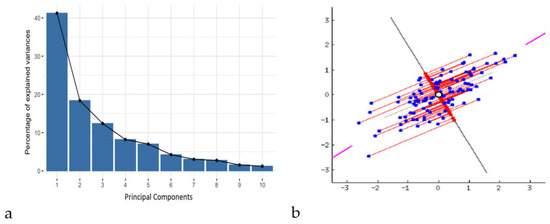
New variables, known as principal components, are created by constructing linear combinations or blends of the original variables. These combinations are made so that the majority of the information contained in the original variables is compressed or squeezed into the first components, while ensuring that these new variables (principal components) remain uncorrelated. For example, a dataset with 10 variables will yield 10 principal components. However, PCA attempts to include as much information as possible in the first principal component, then as much information as possible in the second, and so on, until the result resembles the scree plot given in Figure 1, thus preserving the maximum possible variance within the dataset.

Figure 1. Description of principal components using scree plots (a) and graphical representation of PCA in two-dimensional space (b) [41].

By removing components that contain little information and using the remaining components as new variables, dimensionality can be minimized without losing significant information by organizing the data into primary components. It is crucial to understand that because the primary components are created as linear combinations of the initial variables, they are less interpretable and have no true significance. Principal components, or the lines that capture the majority of the data, are geometric representations of the directions of the data that explain the greatest amount of variance. Here, variance and information are related in that a line’s dispersion of data points increases with the variance it carries, and a line’s information content increases with the dispersion along the line. To put it simply, consider principal components as additional axes that offer the optimal perspective for observing and assessing the data, making the disparities between observations more apparent.

Principal components are designed so that the first principal component explains the greatest amount of variance in the dataset, since there are as many principal components as there are variables in the data. For instance, if the scatter plot of the dataset looks like the one below, the first principal component is the line passing through the origin where the projection of the data points (red dots) is most dispersed, as indicated by the purple line in Figure 1b. Mathematically, this corresponds to the line that maximizes the variance, defined as the average of the squared distances between the origin and the projected points. With the requirement that it be uncorrelated with (i.e., perpendicular to) the first principal component and that it account for the next biggest variance, the second principal component is computed similarly. Namely, the second principal component is then calculated as the line orthogonal (uncorrelated) to the first that captures the next largest variance. This process continues iteratively until all principal components, equal in number to the original variables, are identified. Representation of this explanation is given in Figure 1b.

PCA facilitated the identification of key parameters that contributed significantly to the variance in surface morphology and enabled the differentiation of corrosion behavior under various exposure conditions. The first few principal components captured the majority of the dataset’s variance (80% or more), allowing for effective visualization of sample clustering and trends in morphological evolution due to corrosion. PCA was performed on the datasets of morphological parameter values for detected damages in all samples, measured over each corrosion period. Using this approach, four distinct datasets were created for PCA, each representing a specific corrosion duration. The dimension of datasets varied according to the number of isolated damages on the samples’ surface. The morphology parameters that were investigated were the same in all datasets. The dimension reduction was performed in the two-dimensional PC1–PC2 space of the maximal variance to enable easy visualization of the dataset’s structure (the elements with similar variance generate more or less coherent groups), and emphasize the differences between different material structures. The advantage of the chosen data dimension reduction method was the extraction of morphological parameters, which were the most informative for the resulting PC1–PC2 image, during the same process [38]. PCA was conducted using the Minitab Statistical Software 20 (Product version: Minitab^® 20.4 (64-bit) © 2021 Minitab, LLC (State College, PA, USA). All rights reserved). Before PCA, all morphological parameters were standardized using z-score normalization (mean = 0, standard deviation = 1) to remove scale differences and prevent variables with larger magnitudes from dominating the multivariate analysis.

3. Results and Discussion

3.1. Macrostructure and Microstructure Analysis

The macrostructure and microstructure of X210Cr12 tool steel were investigated over 0–120 days of exposure to a 3.5% NaCl solution using SEM imaging and EDS elemental analysis. SEM examinations were conducted using a 10 μm scale bar to monitor changes in surface morphology and microstructure over time, while EDS enabled detection of compositional trends. These observations provided insights into the progressive degradation of the steel surface in a chloride-rich environment.

It should be noted that EDS provides only elemental information and cannot unambiguously identify specific oxide or hydroxide phases or oxidation states. Therefore, corrosion products are described throughout this section as iron- and chromium-containing oxide or hydroxide species.

Changes in the elemental composition of X210Cr12 tool steel were evaluated before (Table 1) and after exposure to a 3.5% NaCl solution (Figures 3–6) using EDS analysis. Due to the semi-quantitative nature of EDS and its limited accuracy for minor and light elements, particularly carbon, only Fe, Cr, Cl, and O were selected as key elements for a targeted evaluation of localized corrosion effects. Therefore, elements present at low concentrations, such as carbon, were excluded from analysis due to significant measurement inaccuracies (for example, EDS may show approximately 3% instead of the actual 0.4%) [42].

In this analysis, all detectable elements in the EDS spectra were measured, including those originating from the saline environment (Na, Cl, K, Mg, Ca, Sr, Br, F), which may appear due to surface contamination, as well as trace amounts of alloying elements (Si, Mn, Ni, V, Cu, S, Co, and Sn). These elements were detected at concentrations below 1% and have been excluded from further analysis, as they are not expected to significantly influence the alloy’s corrosion mechanisms or fundamental properties. This approach allows for a targeted evaluation of localized corrosion effects by focusing on Fe, Cr, Cl, and O, while minor trace elements are considered negligible in this context.

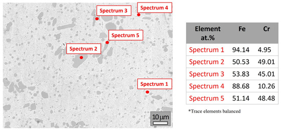
Figure 2 presents selected SEM image and elemental composition of the steel on day zero. The results closely match the original composition (Table 1), with notably reduced levels of impurities such as sulfur and phosphorus.

Figure 2. SEM image and elemental composition (at marked spots) of X210Cr12 tool steel before testing.

The EDS analysis of X210Cr12 reveals a heterogeneous microstructure typical of high-chromium tool steels, consisting of an Fe-rich martensitic matrix with dispersed Cr-rich carbides. Spectra 1 and 4 correspond to an Fe-rich martensitic matrix (~88 and 94 at.%, respectively) with low chromium content (4.95 and 10.26 at.%). The presence of spectra with nearly 1:1 Fe:Cr ratios (e.g., Spectra 2, 3, and 5) indicated the presence of primary Cr-rich carbides, likely of type M₇C₃. Although carbon is not detectable due to the limitations of EDS, the Fe/Cr atomic ratios support the identification of these phases. No oxygen or chloride was detected, indicating a metallic, unoxidized surface. Overall, these results confirm that X210Cr12 is a wear-resistant tool steel, characterized by a martensitic matrix reinforced with hard chromium carbides, consistent with the expected microstructure based on its alloy composition and phase characteristics (see Supplementary Material S1 for a full set of spectra and elemental compositions).

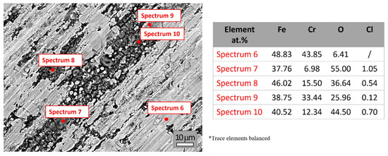
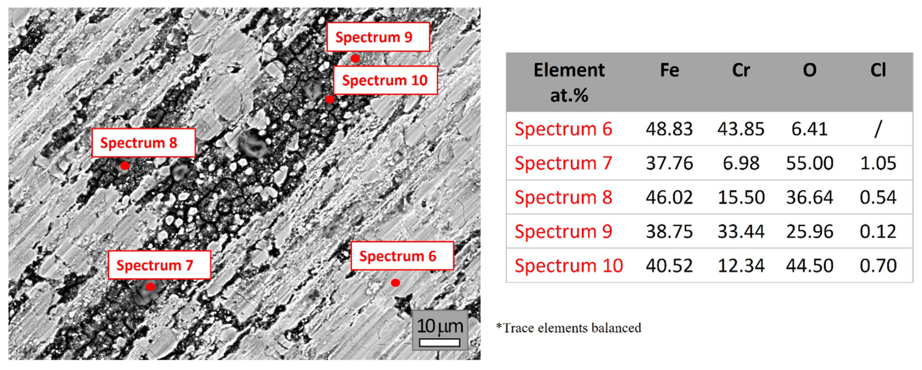
Figure 3 presents the SEM image and elemental compositions (at marked spots) of X210Cr12 tool steel after 30 days of exposure to 3.5% NaCl solution. At first glance, corrosion effects become clearly visible on the surface. Considering the original chemical composition (Table 1) and the EDS elemental composition at the beginning (day zero) shown in Figure 2, the Fe and Cr contents decrease after exposure, while the presence of oxygen detected during EDS analyses (Figure 3) confirms the beginning of the oxidation process. This behavior can be attributed to the chemical reaction between chlorine ions and chromium, which disrupts the integrity of the protective surface layer. The resulting instability creates conditions for a reaction between iron and oxygen, leading to corrosion. EDS analyses also detected the presence of chlorine ions in areas where corrosion has occurred (Spectra 6–10), facilitating localized attack and deeper propagation into the material. A detailed full set of spectra and elemental compositions is provided in Supplementary Material S2.

Figure 3. SEM image and elemental compositions (at marked spots) of X210Cr12 tool steel after 30 days of corrosion.

The surface remains partially metallic in some areas, while others are covered by corrosion products composed mainly of Fe/Cr-containing oxide/hydroxide species. Spectrum 6 exhibits a predominantly metallic surface, consistent with the original composition, suggesting initial oxidation and minimal corrosion. Spectra 7 and 10 show high oxygen levels, suggesting the presence of heavily oxidized areas and the formation of iron- and chromium-containing oxide/hydroxide species. Spectrum 7 contains elevated Cl and reduced Cr at the surface, suggesting chloride-induced localized corrosion and degradation of the protective surface layer. In contrast, Spectrum 10, due to its notable chromium content and minor chloride presence, indicates the development of an Fe-Cr-rich oxide/hydroxide layer. Spectra 8 and 9 indicated a moderately corroded area, characterized by a mixture of metallic and oxidized areas, while Spectrum 9 showed a relatively high content of Cr, possibly due to the presence of localized Cr-rich oxide/hydroxide layers. Comparison of the elemental composition before and after 30 days of exposure provides clear evidence of degradation. The iron content decreases significantly due to dissolution, whereas oxygen and chlorine appear after exposure, confirming the formation of oxide/hydroxide layers and chloride ion penetration. The Cr content varies considerably, reflecting localized breakdown or retention of the protective surface layer. These results confirm that X210Cr12 tool steel undergoes heterogeneous corrosion in 3.5% NaCl solution, characterized by areas of severe oxidation and chloride-induced localized attack.

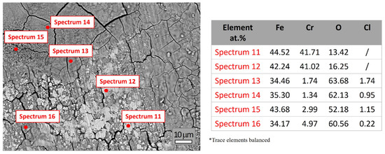
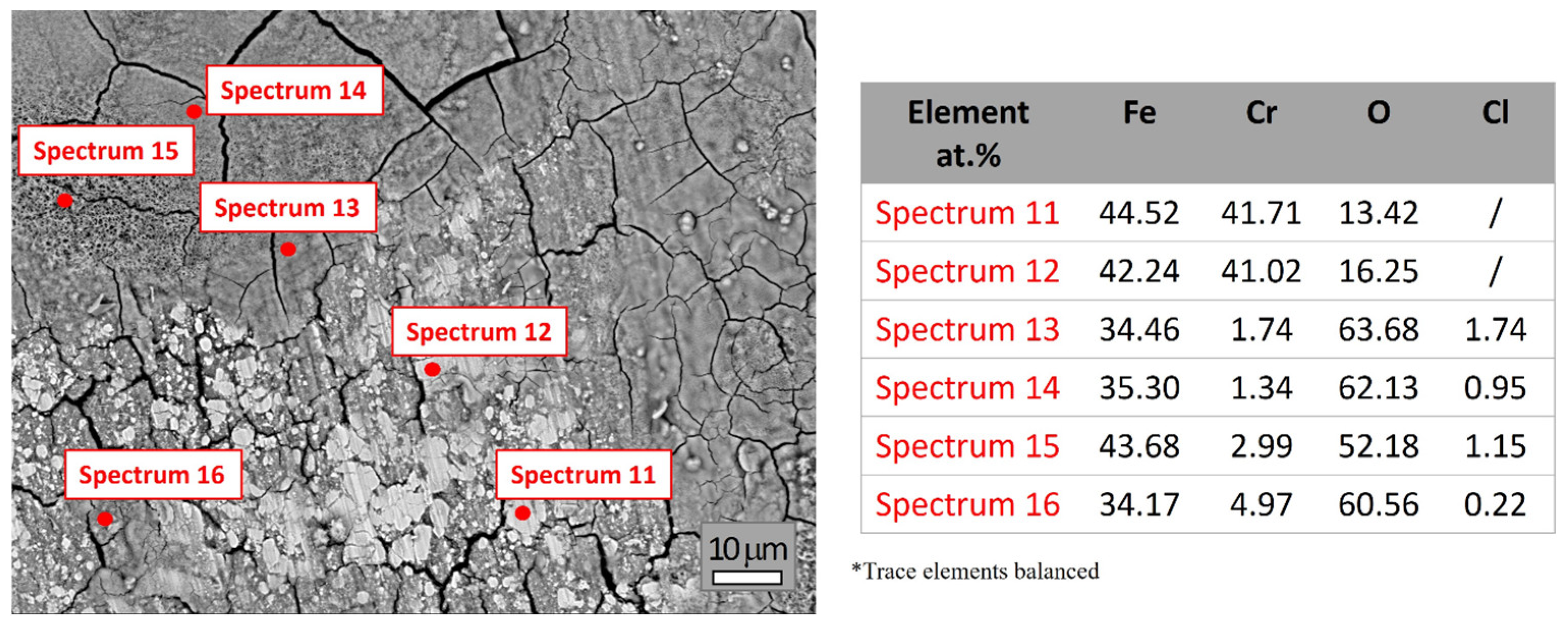
The elemental composition obtained from Spectra 11–16 (Figure 4; see Supplementary Material S3 for the full set of spectra and elemental compositions) highlights the significant surface heterogeneity of the X210Cr12 tool steel after 60 days of exposure to a 3.5% NaCl solution, indicating progressive corrosion and oxide/hydroxide formation. The measured oxygen contents increase more notably than those reported in Figure 3, suggesting more advanced surface oxidation. Chromium contents are generally lower compared to Figure 3, indicating the degradation or absence of the protective surface layer across most of the sample surface. Additionally, localized Cl enrichment areas were observed in several regions, suggesting the role of chloride ions in promoting more advanced oxidation and continued breakdown of the protective surface layer.

Figure 4. SEM image and elemental composition (at marked spots) of X210Cr12 tool steel after 60 days of corrosion.

Spectra 11 and 12 are characterized by high Fe content (~42–44 at.%) and Cr content (~41 at.%), with moderate oxygen levels (~13–16 at.%), indicating that the analyzed surface areas are only partially oxidized, likely consisting of a thin layer of mixed Fe- and Cr-containing oxide/hydroxide species. Spectra 13 and 14 exhibit significantly higher oxygen content (~62–64 at.%), accompanied by a strongly reduced content of Cr (~1.3–1.7 at.%) and Fe (~34–35 at.%), reflecting pronounced surface degradation and formation of Fe-rich oxide/hydroxide products. The presence of chlorine (up to 1.74 at.%) in these spectra indicated localized areas of intense corrosion, likely due to chloride-induced pitting. The composition of these areas suggests dominance of Fe-rich oxide/hydroxide layers, with only minimal residual metallic content. Spectra 15 and 16 showed oxygen contents exceeding 50 at.%, Fe between 34 and 44 at.%, and low Cr (2.99 and 4.97 at.%), indicating more advanced oxidation and partial degradation of the Cr-rich passive layer in some areas, allowing deeper corrosion. The presence of Cl further confirms the active role of chloride ions in promoting and continuing chloride-induced localized corrosion.

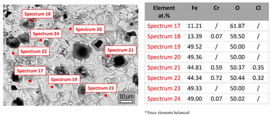
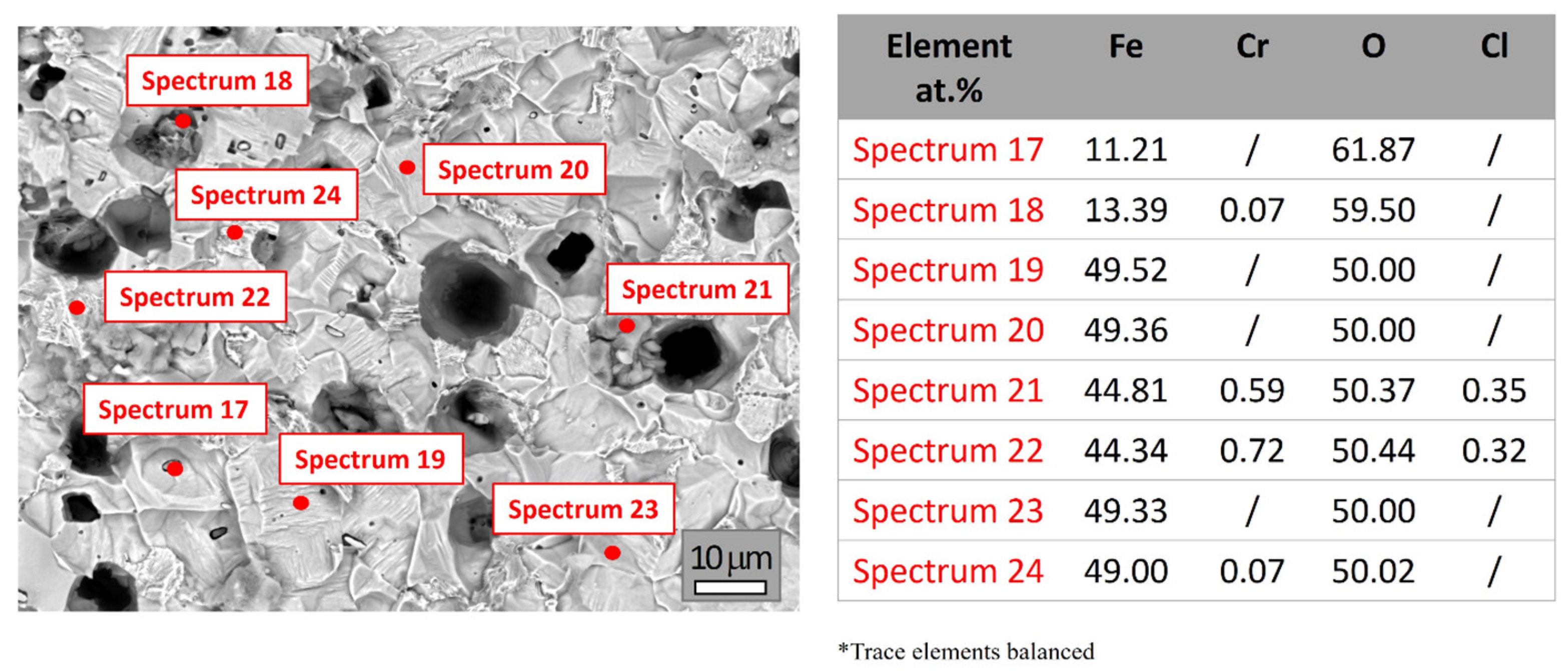
Figure 5 shows the SEM image and elemental compositions (at selected spots, Spectra 17–24) of X210Cr12 tool steel after 90 days of exposure to 3.5% NaCl. The microstructure indicates progressive corrosion with significant pitting compared to earlier conditions. High oxygen levels detected by EDS (~50–62 at.%), along with the near absence of surface chromium (Cr), often below detection or <1 at.% in most spectra, indicated extensive corrosion across the steel surface, consistent with the formation of iron-rich oxide/hydroxide species as the primary corrosion products. Iron (Fe) is present in varying amounts, from ~11 to ~49 at.%, suggesting highly heterogeneous corrosion across the surface. All individual spectra and detailed elemental analyses are provided in Supplementary Material S4.

Figure 5. SEM image and elemental composition (at marked spots) of X210Cr12 tool steel after 90 days of corrosion.

Spectra 17 and 18 indicated severe corrosion areas due to very low Fe (~11 at.%) and high O (~60 at.%), suggesting localized pitting and deposition. However, Spectra 17 and 18 also revealed elevated concentrations of sulfur (S), manganese (Mn), and copper (Cu). This suggests the presence of corrosion products possibly associated with residual inclusions or locally deposited species on the oxidized surface. Spectra 19–24 represented more stable areas, showing Fe/O ratios near 1:1 (~49 at.% each), typical of thick iron-rich oxide/hydroxide layers. Spectra 19, 20, 23, and 24 showed higher Fe content (~49 at.%) and moderate oxygen, suggesting the formation of a relatively stable oxide layer. Spectra 21 and 22 exhibited moderate Fe and O levels, along with Cl, while Cr was nearly absent in all spectra, confirming extensive selective leaching from the surface.

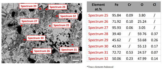
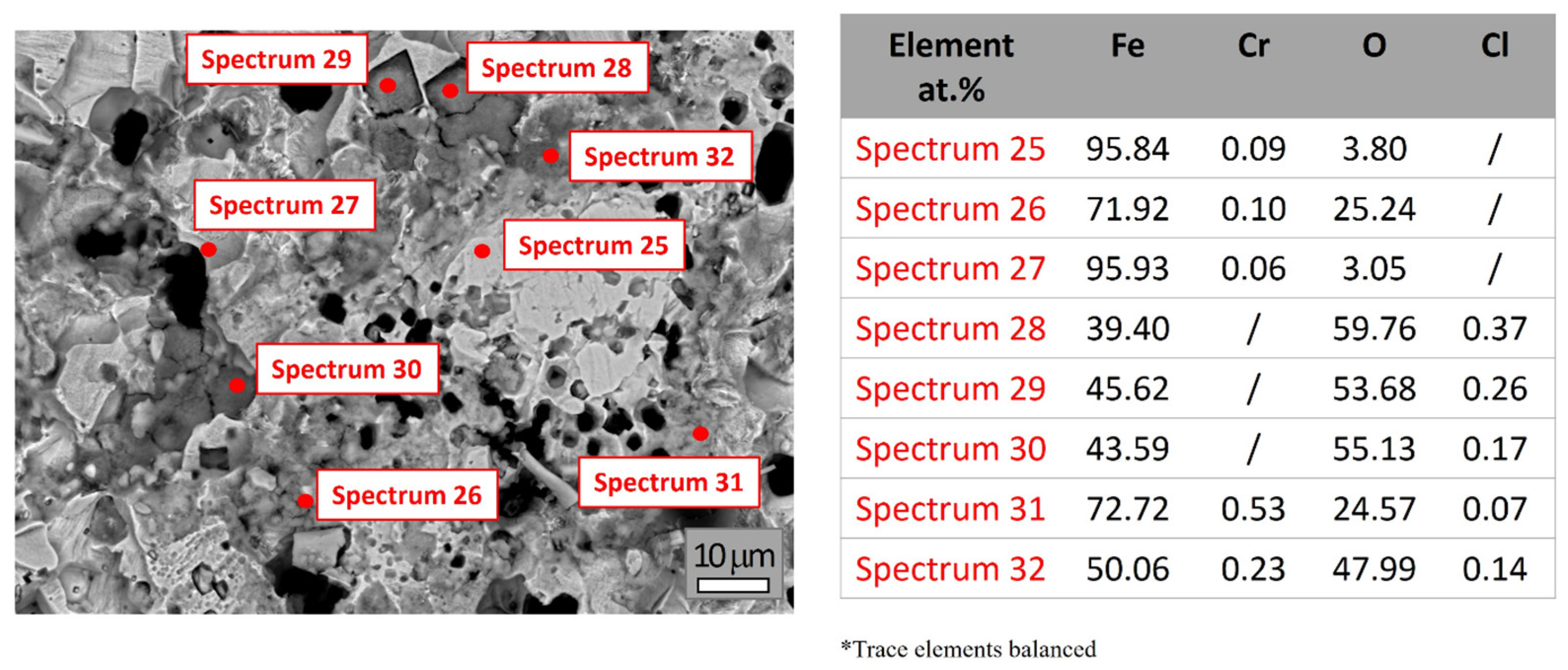
Figure 6 shows the SEM image and elemental composition (at marked spots) of X210Cr12 tool steel after 120 days of exposure. The EDS analysis (Spectra 25–32) reveals pronounced surface heterogeneity, significant oxidation and corrosion development, with pitting corrosion becoming predominant. EDS analyses given in Figure 6 showed the dominant presence of Fe and O. Cr values ranged between 0.06 and 0.53 at.%, just over the detection limit, demonstrating significant chromium depletion after prolonged exposure. A detailed full set of spectra and elemental compositions is provided in Supplementary Material S5.

Figure 6. SEM image and elemental composition (at marked spots) of X210Cr12 tool steel after 120 days of corrosion.

Spectra 25 and 27 exhibited high iron content (>95 at.%) and low oxygen levels (~3 at.%), suggesting the presence of regions with minimal corrosion or areas where corrosion products were locally removed. In contrast, Spectra 28–30 showed elevated oxygen concentrations (53–60 at.%) and reduced iron (~39–46 at.%), revealing the presence of thick Fe-rich oxide/hydroxide layers. Spectra 31 and 32 reflected intermediate stages, with iron ranging from ~50–72 at.% and oxygen from ~24–48 at.%, demonstrating partial oxide/hydroxide layer development. The content of Cr decreases progressively with exposure time in a solution of NaCl, reaching as low as 0.06 at.% in certain areas, confirming continued selective leaching from the surface and breakdown of the initially protective Cr-rich surface layer after prolonged exposure.

Overall, the obtained results provide clear evidence of progressive corrosion, selective leaching of alloying elements, and heterogeneous oxide/hydroxide formation. The EDS analysis reveals advanced surface degradation of the X210Cr12 tool steel in a chloride-rich environment. The chromium content decreased markedly over time, dropping from an initial value of up to 49 at.% to less than 0.7 at.% after 60 days of exposure. This decline indicates selective leaching due to the breakdown of the initially protective Cr-rich surface layer. Simultaneously, the oxygen content increases significantly, reaching 50–60 at.% in the later stages, which is consistent with the formation of iron- and chromium-containing oxide hydroxide species and the transition from a metallic to an oxidized surface. The analyzed spectra demonstrate pronounced surface micro-heterogeneity after prolonged exposure to NaCl solution, with areas ranging from minimally corroded to heavily oxidized, reflecting the pitting susceptibility of the tool steel in NaCl solutions.

3.2. Corrosion Evaluation

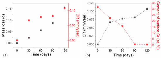
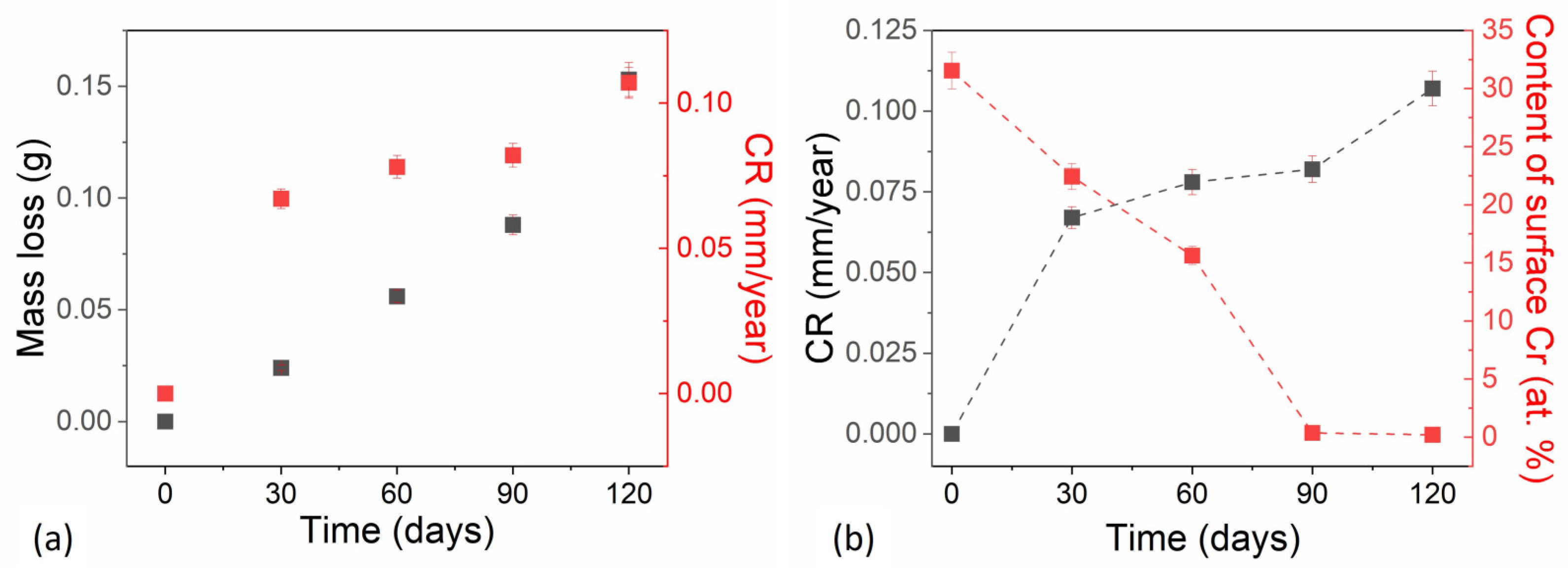
Figure 7a shows the cumulative mass loss and corrosion rate of X210Cr12 tool steel over an immersion period in a 3.5% NaCl solution, simulating a marine-like environment. Additionally, Figure 7b shows a correlation plot that presents the evolution of key parameters, the corrosion rate, and chromium content depletion as a function of immersion time in 3.5% NaCl solution. Values of chromium content are extracted from Figure 2, Figure 3, Figure 4, Figure 5 and Figure 6, which present the average values of different spectra for each immersion period. This is necessary because individual points varied significantly depending on whether the EDS spot was in a metallic area or an oxide. Mass loss measurements were performed in three replicates on a single high-chromium tool steel sample to ensure reproducibility. The average and standard deviation of these measurements are reported in Supplementary Material S6, Table S1. The results reveal a progressive corrosion process, with material degradation increasing over time, demonstrating the limited resistance of this steel to chloride-induced corrosion.

Figure 7. Changes in the corrosion erosion parameters over time. (a) Mass loss, CR vs. Time. (b) CR, Content of surface Cr vs. Time.

Cumulative mass loss increased steadily throughout the test period, with a slight acceleration in later stages. During the first 30 days, mass loss was minimal (0.024 g), suggesting that the initial presence of a chromium-rich passive film or early corrosion products temporarily limited corrosion. Between 60 and 90 days, mass loss continued to increase at a moderate rate, indicating sustained but controlled corrosion activity. A pronounced increase occurred between 90 and 120 days, with mass loss rising from 0.088 g to 0.153 g, larger than in earlier intervals. This jump suggests accelerated corrosion, possibly due to passive film breakdown or the initiation of localized corrosion mechanisms such as pitting, which expand the surface area exposed to the corrosive electrolyte.

The corrosion rates (CRs) of X210Cr12 tool steel in 3.5% NaCl were calculated from mass loss measurements. Values represent the average of three independent measurements, and the corresponding standard deviations are reported in Supplementary Material S7; Table S2. The corrosion rate data illustrate the corrosion dynamics, showing a generally increasing but not linear trend. The results suggest that the corrosion process becomes more aggressive over time, with a gradual intensification of corrosion.

In the first 30 days, the corrosion rate remained low (0.067 mm/y), consistent with a stable Cr-rich passive layer typical of high-chromium steels, which provides initial protection against corrosion. Alternatively, early corrosion products may form a temporary barrier that slows further material dissolution. Between 60 and 90 days, a slight increase in the corrosion rate to 0.082 mm/y suggested the initiation of passive film degradation under chloride ion attack. This behavior may reflect temporary stabilization, possibly due to the partial reformation of a protective layer or experimental variability.

A pronounced acceleration in corrosion was observed between 90 and 120 days, during which the corrosion rate increased sharply to 0.107 mm/y, indicating accelerated material loss. This rise is indicative of localized corrosion, likely driven by pitting corrosion, which becomes a prevalent mechanism in chloride-rich environments once the Cr-rich passive layer is compromised. While corrosion rates below 0.1 mm/year are generally acceptable for many industrial applications, the value of 0.107 mm/year at 120 days suggests that prolonged exposure could result in substantial material degradation over extended service periods.

Figure 7b, based on the average chromium content from all EDS spectra per immersion period, indicates that surface chromium content decreases sharply from approximately 49 at.% initially to below 1 at.% by 90 days, and remains at this low level at 120 days, suggesting the loss of the protective passive layer. Trends observed after 90 days, including a high degradation area (Figure 7b), low chromium content, and rising corrosion rates, indicated a transition to the defect coalescence and acceleration stage of corrosion, where pit merging and chromium depletion drive rapid metal loss. The corrosion rates (CRs) calculated from mass loss represent the average material loss normalized to the exposed surface area and exposure time. Therefore, these values should not be interpreted as local pit penetration rates, particularly because the SEM observations demonstrate pronounced localized corrosion.

3.3. Corrosion-Induced Defects and Their Surface Morphology

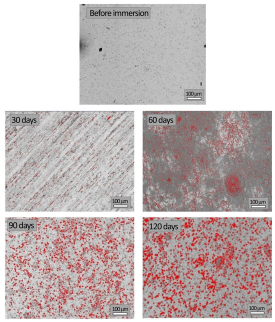
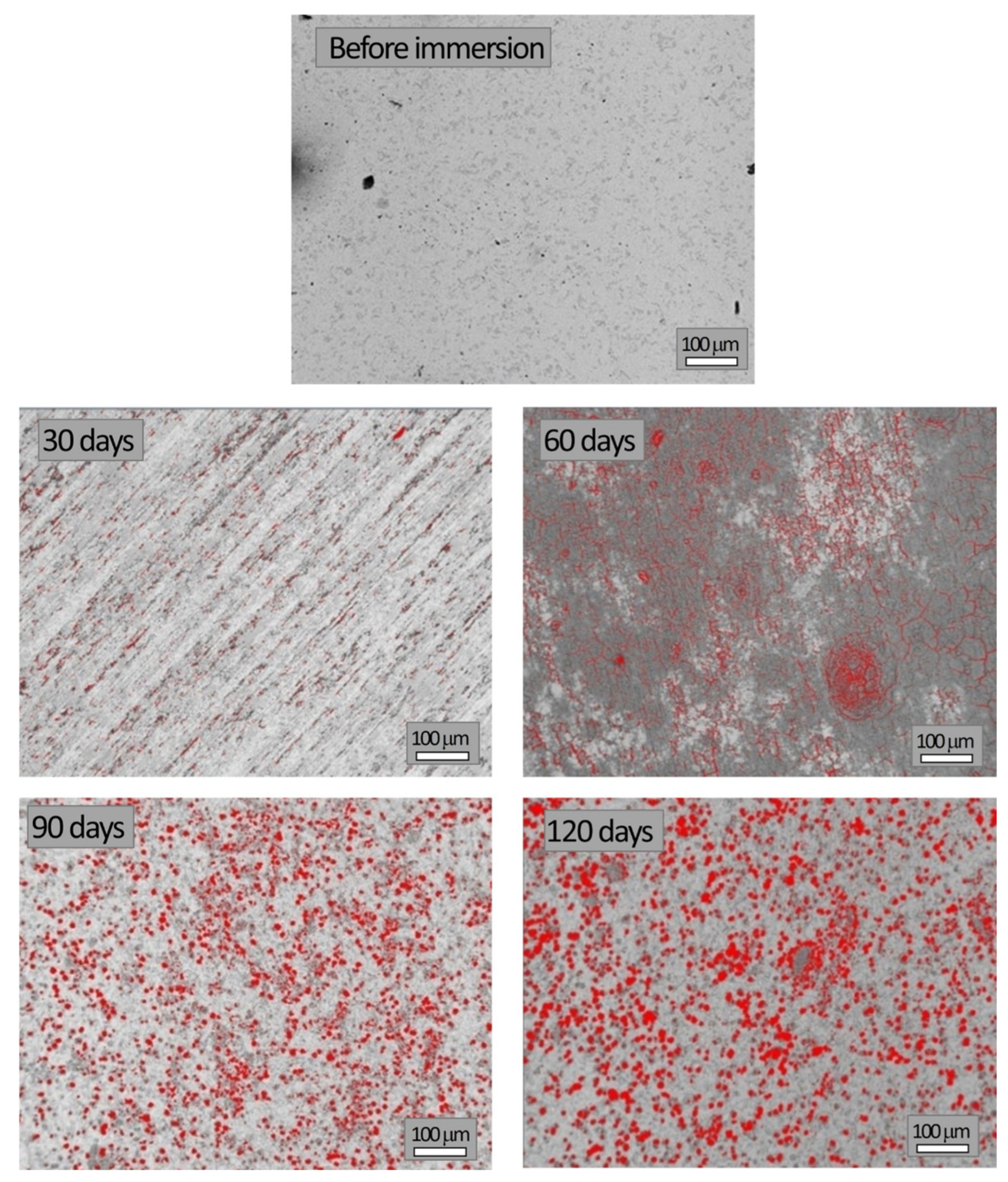
SEM images of the studied samples before and during corrosion testing in NaCl solution, which were used to quantify the surface degraded area, are shown in Figure 8. The same magnification (100 μm scale bar) was used to enable direct comparison of images obtained at different immersion times.

Figure 8. Images of the sample during different immersion times.

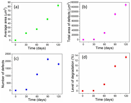
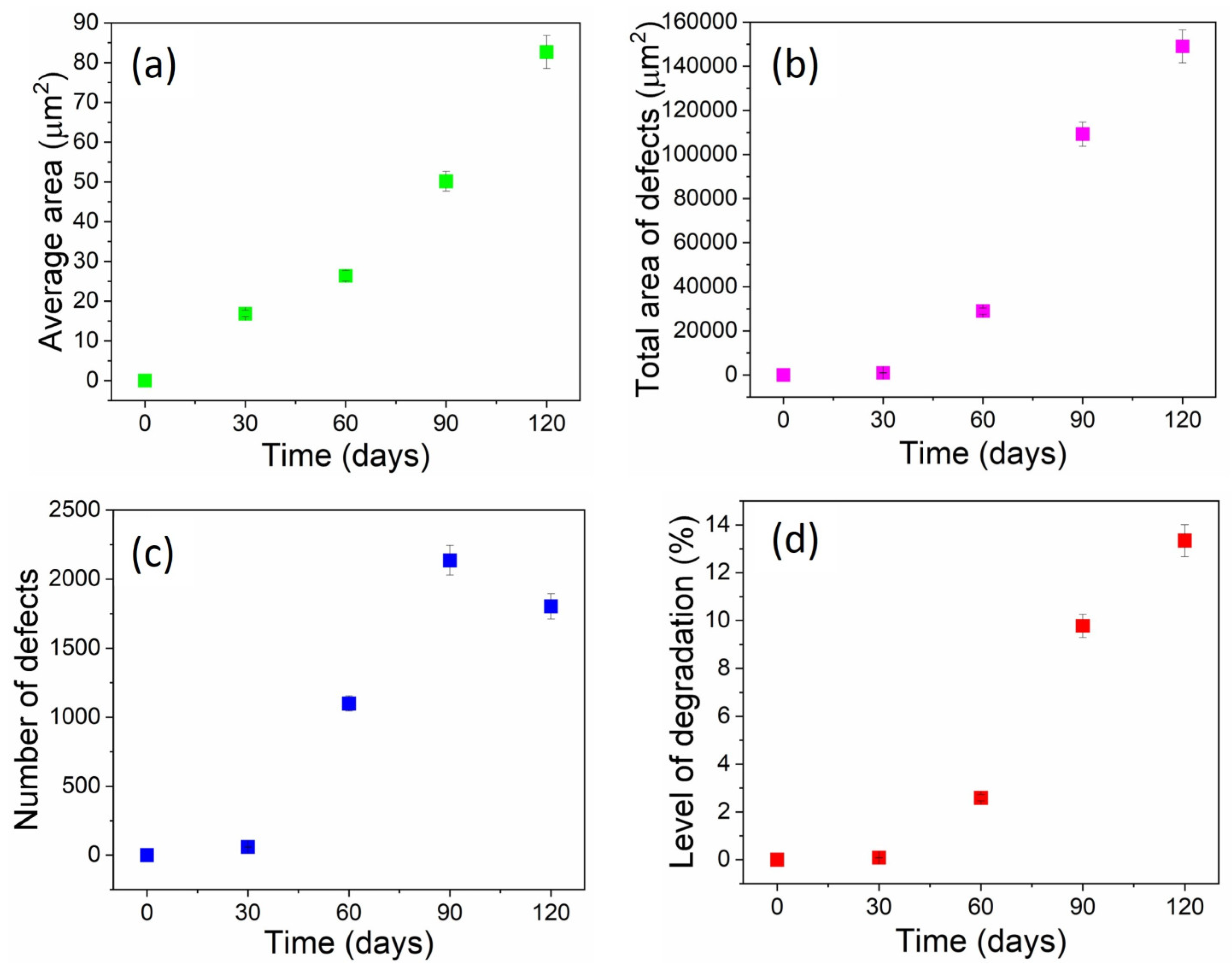
Image analysis was performed using IPP to quantify the average degraded area, total degraded area, number of defects, and overall degradation level, while the results are given in Figure 9.

Figure 9. Results of image analysis: (a) average area of defects, (b) total area of defects, (c) number of defects, and (d) level of degradation versus time of immersion.

SEM analysis revealed a distinct progression of corrosion in the surface morphology of X210Cr12 steel during immersion in a 3.5% NaCl solution. After 30 days, only a few small, isolated pits were visible (59), covering 0.089% of the observed area. These pits likely initiated at the carbide–matrix interfaces and chromium-depleted zones, which serve as favored sites for passive film breakdown in a chloride-containing environment. By 60 days, pit density increased sharply (1099 defects, 2.59% degraded area), indicating active nucleation. Between 60 and 90 days, both the number of pits and their average size increased significantly, demonstrating simultaneous nucleation and pit growth, ultimately affecting 9.78% of the surface. After 90 days, the number of defects decreased despite further growth in average pit size, suggesting the occurrence of pit coalescence. At 120 days, large merged cavities dominated the surface, with the degraded fraction reaching 13.34%. This morphological evolution from early-stage nucleation to growth and eventual coalescence reflects the typical pitting corrosion mechanism in high-carbon, high-chromium tool steels exposed to chloride-rich environments.

The applied methods revealed three distinct stages of the corrosion process: an incubation stage, where the passive film remained largely unchanged, with only isolated pit occurrences; a stage of pit propagation, which implied growth of existing pits accompanied by the formation of new ones and breaking of the passive film at the surfaces; and a coalescence and acceleration stage, characterized by merging of the already existing pits, leading to accelerated metal loss, with Cr almost entirely leached from the surface.

3.4. Principal Component Analysis

A set of morphological descriptors, including Area, Diameter_max, Diameter_min, Diameter_mean, Radius_max, Radius_min, Radius Ratio, Roundness, Perimeter_ellipse, and Perimeter_ratio, was determined from micrographs processed by Image-Pro Plus 6.0. These parameters quantify the size, shape, and geometric proportions of the analyzed features, which are pits and defects. As a result of image analysis measurements, large datasets are generated for each parameter at different immersion times. To explore relationships among the variables and reduce the complexity of the obtained multidimensional dataset, Principal Component Analysis (PCA) was applied. This method transforms correlated variables into a smaller set of independent principal components (PCs), enabling the identification of key morphological patterns and relationships among the variables. Namely, it transforms the correlated morphological parameters into principal components (PCs), which are linear combinations of the original variables. The first few PCs (e.g., PC1 and PC2) capture the majority of the variance in the data, allowing for easier interpretation of trends and groupings.

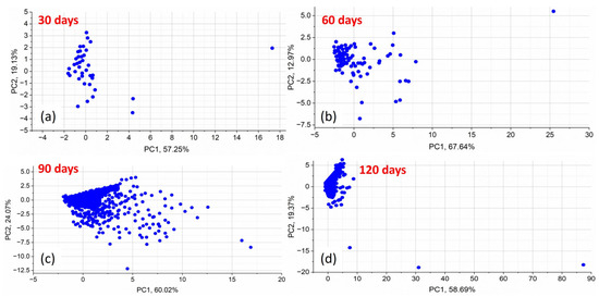
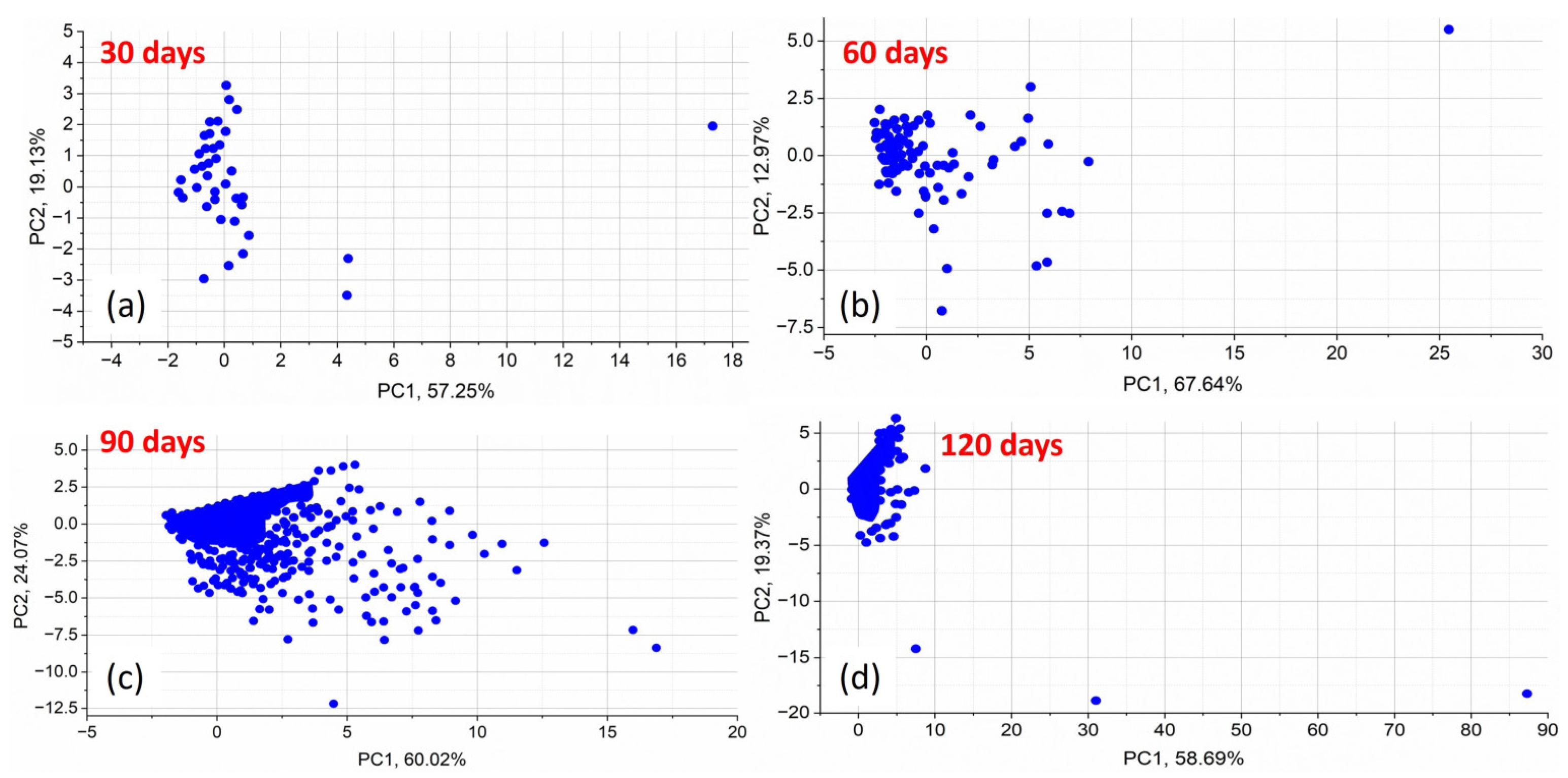
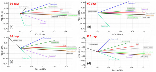
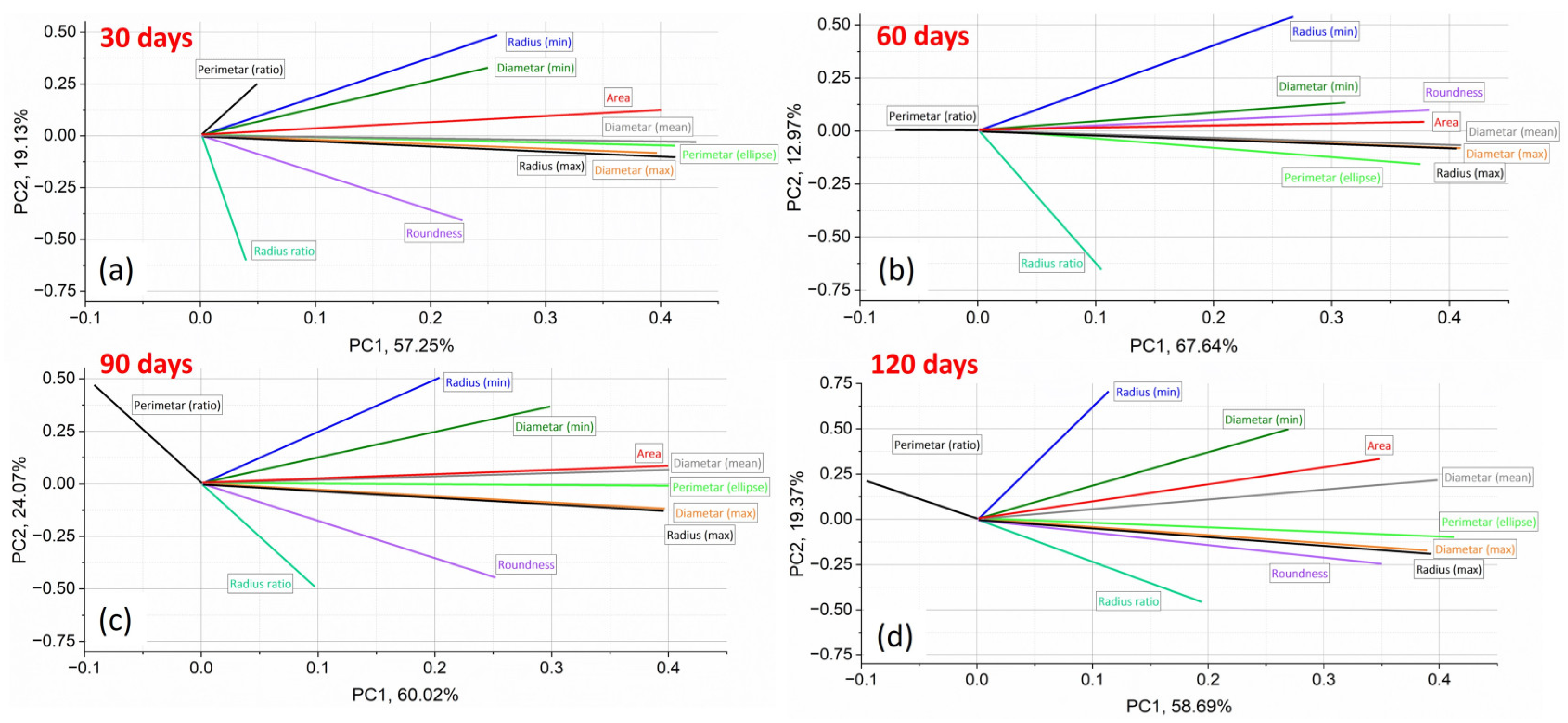
Figure 10 and Figure 11 present the PCA results, visualizing morphological changes in corrosion defects over immersion times. Figure 10 shows the score plots in the space of maximal variance of the morphological parameters used to describe corrosion at different immersion times. Figure 11 presents the loading plots in the PC1–PC2 space of maximal variance for the same parameters, illustrating their contribution of each morphological descriptor to the observed trends.

Figure 10. Score plots in PC space for morphology parameters used to describe corrosion at (a) 30 days, (b) 60 days, (c) 90 days, and (d) 120 days immersion.

Figure 11. Loading plots in PC1–PC2-space of maximal variance showing the contribution of morphology parameters for (a) 30 days, (b) 60 days, (c) 90 days, (d) 120 days of immersion.

PCA provides insight into the evolution of morphological parameters of corrosion defects during immersion. Figure 10 presents the score plots in the PC1–PC2 space for immersion times of 30, 60, 90, and 120 days, with each point representing a sample in the reduced PCA space. The distribution of scores reveals clear changes in corrosion morphology over time. At 30 days, the samples form a compact cluster, indicating similar corrosion patterns and low variability in defect geometry (Stage 1). At 60 and 90 days, increased dispersion along PC1 reflects greater variability in defect size and shape (Stage 2). By 120 days, the scores become more dispersed along both PC1 and PC2, indicating advanced degradation characterized by increased morphological irregularity and surface heterogeneity (Stage 3). Detailed PCA variance data are provided in Supplementary Material S8.

The PCA loading plots (Figure 11) reveal a clear evolution of the dominant morphological descriptors with exposure time, based on the relative contribution of each morphological parameter to the principal components and reflecting the transition between different corrosion stages. The loading plots indicate how strongly each morphological descriptor influences PC1 and PC2; parameters located farther from the origin have a greater impact on the variance captured by the principal components. These plots enable the identification of morphological descriptors that drive the observed corrosion trends at each stage, clarifying which parameters are most responsible for these differences.

In the early exposure period (30 and 60 days), the largest proportion of variance captured by the first principal component (strongly aligned with PC1) was primarily governed by size-related parameters, including pit Area, Diameter_mean/max, Radius_max, and Perimeter_ellipse. However, in the early-to-mid-stages (60 days), shape-related descriptors such as Roundness and Radius Ratio showed a weaker association, mainly with PC2, indicating the initiation of minor geometric changes. At this stage, corrosion evolution is dominated by pit growth and expansion, while pit geometry remains relatively consistent. These patterns suggest that early corrosion is mainly characterized by an increase in defect size. Most precisely, early stages may exhibit uniform corrosion with smaller, more regular features, as reflected in descriptors like Area or Roundness.

With prolonged exposure (90 and 120 days), shape-related descriptors progressively gain importance in the PCA loadings. At 90 days, the transition was obvious since size parameters still strongly influence PC1, but Roundness and Radius Ratio showed increased contributions in PC2, reflecting the importance of complex shape alterations and more irregular surface morphologies. At 120 days, while Area and Diameter remained significant in PC1, Roundness and Radius Ratio became highly informative, along with Perimeter Ratio, indicating coalescence of pits and a loss of regularity. In particular, Roundness and Radius ratio showed increased contributions, reflecting the development of irregular, elongated, and interconnected corrosion features caused by pit interaction and coalescence.

Although size-related parameters remain influential, the increasing contribution of shape-related descriptors indicates a transition from isolated pit growth toward defect interaction, morphological complexity, and greater surface heterogeneity.

Overall, the PCA results indicate that early corrosion is primarily size-driven, whereas prolonged exposure promotes shape evolution and pit interaction, consistent with the observed chromium depletion and accelerated material degradation.

3.5. Mechanism of Corrosion Evolution in 3.5 wt.% NaCl Solution

To elucidate the synergistic mechanism between chromium-rich passive film degradation and Cl⁻ penetration, the phenomenon can be interpreted through established electrochemical theories and the relevant literature, which emphasize the critical role of chloride ions in destabilizing the initially protective surface layer (commonly associated with Cr₂O₃) and triggering localized corrosion. The electrochemical processes involved, including the anodic dissolution of metal in the presence of chloride ions, have been extensively studied and are supported by theories of localized breakdown and repassivation mechanisms [2,43,44,45,46]. These studies explain how chloride ions, due to their aggressive nature, can penetrate and destabilize the passive oxide layer, initiating corrosion at specific sites on the steel’s surface.

The corrosion evolution of X210Cr12 tool steel in a chloride-rich environment can be interpreted through the combined analysis of SEM morphology, EDS elemental trends, mass loss measurements, and PCA of morphological descriptors. These complementary methods consistently indicate a transition from initial passive film degradation to pit growth and, finally, pit coalescence and accelerated corrosion. The electrochemical response of the steel surface under these conditions can be analyzed through models that describe chloride-induced local depassivation, followed by the formation of pits that are more active than the surrounding passive material [45,46,47,48].

In the early stage (30–60 days), corrosion is initiated by local breakdown of the chromium-rich passive film under chloride ion attack. Chloride ions adsorb on the passive film and promote local depassivation, particularly at microstructural heterogeneities such as carbide–matrix interfaces and chromium-depleted regions. SEM observations reveal small, isolated pits, while EDS shows the initial decrease in surface chromium content accompanied by the appearance of oxygen and chlorine, confirming the beginning of localized corrosion. In this stage, PCA results show that size-related morphological descriptors dominate the variance captured by PC1, indicating that corrosion is primarily governed by pit nucleation and dimensional growth, while pit geometry remains relatively regular. Electrochemical studies have shown that the corrosion current density increases at these localized sites due to the destabilization of the oxide film, leading to the initiation of pitting corrosion [39,43]. Figure S8 in Supplementary Material S9 shows a higher-magnification SEM image of pit nucleation sites at carbide–matrix interfaces, highlighting early-stage corrosion features of X210Cr12 tool steel after immersion in 3.5% NaCl solution for 60 days.

With increasing exposure time (around 60–90 days), pit growth accelerates and new pits continue to nucleate, leading to a higher defect density and increased degraded area. EDS results demonstrate a pronounced decrease in chromium content and increasing oxygen concentration, reflecting progressive degradation of the Cr-passive film and the formation of iron oxides and hydroxides. The presence of chlorine in corroded regions indicates sustained chloride penetration and stabilization of localized anodic dissolution within pits. PCA reveals the emergence of shape-related descriptors with increased contribution to PC2, reflecting the beginning of pit shape distortion and growing surface heterogeneity. This stage represents the transition from predominantly size-controlled corrosion to combined size and shape evolution. Electrochemical studies emphasize that chloride ions not only disrupt the passive film but also facilitate the formation of aggressive localized microenvironments, where pitting becomes self-sustaining and growth accelerates [49,50,51].

In the advanced stage (90–120 days), extensive chromium depletion was observed by EDS, with chromium contents approaching the detection limit, confirming the near-complete loss of a continuous Cr-protective film. SEM images revealed pronounced pit coalescence and the formation of large, irregular, and interconnected corrosion cavities. Thick iron oxide/hydroxide layers dominate the surface, while chloride ions remain present in active corrosion zones, sustaining localized dissolution and preventing repassivation. In this stage, PCA showed a strong contribution of shape-related descriptors, indicating that morphological irregularity, pit interaction, and defect coalescence become the dominant features of surface degradation. Although size-related parameters remain relevant, the increasing influence of shape descriptors reflects a shift toward highly heterogeneous corrosion morphology and accelerated material loss. Electrochemical models suggest that once the passive film is compromised and pit coalescence occurs, the steel surface experiences a rapid increase in the corrosion rate, further exacerbated by the interaction between pits and the continuous chloride ion penetration [52,53,54].

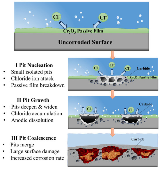
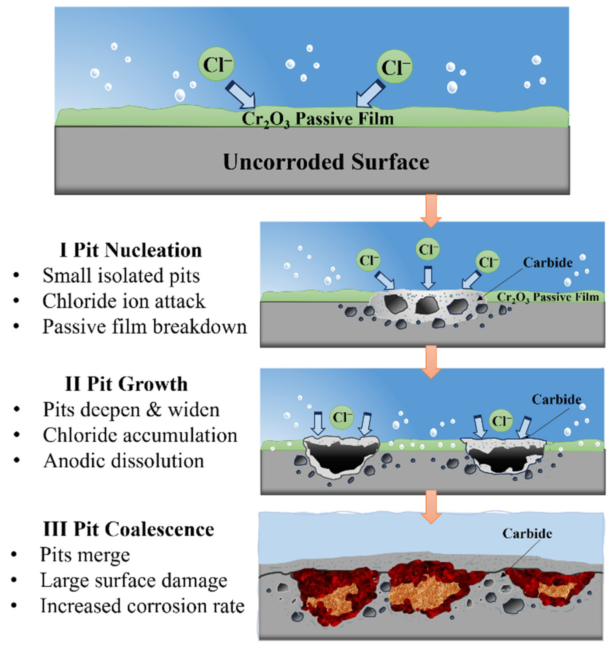
Overall, the integrated SEM–EDS–PCA demonstrates that corrosion of X210Cr12 tool steel in 3.5% NaCl solution proceeds through three distinct stages: initial surface degradation and pit nucleation, associated with localized disruption of the protective surface layer; pit growth and propagation, associated with sustained chloride exposure and the progressive development of corrosion products; and pit coalescence and acceleration, characterized by increasing surface damage, interaction between neighboring defects, and the development of highly irregular corrosion morphologies. A schematic diagram illustrating the three stages of the corrosion process is shown in Figure 12.

Figure 12. A schematic diagram of three corrosion stages.

This mechanistic interpretation explains the observed transition in PCA dominance from size-related descriptors at early stages to shape-related descriptors at advanced corrosion stages and is consistent with the measured increase in mass loss and the corrosion rate at prolonged exposure times. The synergistic effect of Cr-rich passive film damage and chloride ion intrusion can be better understood through electrochemical perspectives, where chloride-induced depassivation leads to active corrosion sites with increasing surface heterogeneity and mass loss over time [47,53,54].

It should be emphasized that the identification of specific corrosion-product phases remains tentative, as it is based solely on EDS elemental trends. Complementary phase-identification techniques (e.g., XRD, Raman spectroscopy, FTIR, or XPS) would be required for definitive confirmation. The mechanistic interpretation presented here is therefore proposed based on the observed surface morphology, elemental composition, and mass-loss trends. Although electrochemical measurements were not conducted in the present study, they are expected to provide quantitative insights into local corrosion rates and passive film destabilization, and will be the subject of forthcoming investigations.

4. Conclusions

This study investigated the corrosion progression of X210Cr12 tool steel during immersion in a 3.5% NaCl solution representing a marine-like chloride environment, through the combined application of mass loss measurements, SEM/EDS analysis, quantitative image analysis, and PCA. The findings revealed progressive surface degradation, with cumulative mass loss increasing from 0.024 g after 30 days to 0.153 g after 120 days and the corrosion rate increasing from 0.067 to 0.107 mm/year.

Image analysis revealed three distinct stages of surface degradation: an initial incubation period dominated by the nucleation of isolated pits, a propagation stage characterized by the simultaneous nucleation and growth of multiple pits, and a final coalescence stage where pits merged into large cavities, associated with accelerated metal loss. The degraded surface fraction area increased from 0.089% at 30 days to 13.34% at 120 days. EDS analysis showed pronounced depletion of surface chromium and increasing oxygen content in corroded regions. PCA indicated that size-related descriptors (Area, Diameter_max, Radius_max, and Perimeter_ellipse) were dominant indicators at the early stages of corrosion, while shape-related descriptors (Roundness, Radius Ratio, and Perimeter_ratio) became more significant at advanced stages.

The integration approach of SEM/EDS, image analysis, and PCA provides a reliable framework for quantitatively monitoring corrosion-induced surface defects and identifying morphological descriptors associated with different stages of corrosion. However, the study was performed in a simplified NaCl environment, and the corrosion-product phases and electrochemical behavior were not directly characterized. Future studies will involve real seawater conditions, complementary phase characterization, and electrochemical measurements.

References

- Raja, P.B.; Ismail, M.; Ghoreishiamiri, S.; Mirza, J.; Ismail, M.C.; Kakooei, S.; Rahim, A.A. Reviews on corrosion inhibitors: A short view. Chem. Eng. Commun. 2016, 203, 1145–1156. [Google Scholar] [CrossRef] [Scilit]
- Xia, D.-H.; Deng, C.-M.; Macdonald, D.; Jamali, S.; Mills, D.; Luo, J.-L.; Strebl, M.G.; Amiri, M.; Jin, W.; Song, S.; et al. Electrochemical measurements used for assessment of corrosion and protection of metallic materials in the field: A critical review. J. Mater. Sci. Technol. 2022, 112, 151–183. [Google Scholar] [CrossRef] [Scilit]
- Roberge, P.R. Handbook of Corrosion Engineering; McGraw-Hill Education: New York, NY, USA, 2019. [Google Scholar]
- Xie, W.; Shiu, W.Y.; Mackay, D. A review of the effect of salts on the solubility of organic compounds in seawater. Mar. Environ. Res. 1997, 44, 429–444. [Google Scholar] [CrossRef] [Scilit]
- Peng, W.; Duan, T.; Hou, J.; Guo, X.; Zhang, Y.; Ma, L.; Yu, M.; Xin, Y.; Xing, S.; Zhang, H. Electrochemical corrosion behavior of high strength steel in simulated deep-sea environment under different hydrostatic pressure. J. Mater. Res. Technol. 2023, 23, 2301–2316. [Google Scholar] [CrossRef] [Scilit]
- Mazilu, A.; Benea, L.; Axente, E.R. Monitoring and evaluation of the corrosion behavior in seawater of the low-alloy steels BVDH36 and LRAH36. Int. J. Mol. Sci. 2024, 25, 6405. [Google Scholar] [CrossRef] [Scilit] [PubMed]
- Yu, X.; Al-Saadi, S.; Zhao, X.L.; Raman, R.K.S. Electrochemical investigations of steels in seawater sea sand concrete environments. Materials 2021, 14, 5713. [Google Scholar] [CrossRef] [Scilit] [PubMed]
- Riccioli, F.; Gabrielsen, Ø.; Høgsæt, I.S.; Barros, P.S.; Pahlavan, L. Corrosion-fatigue damage identification in submerged mooring chain links using remote acoustic emission monitoring. Mar. Struct. 2024, 98, 103685. [Google Scholar] [CrossRef] [Scilit]
- Lotsberg, I. Assessment of internal defects in flush ground butt welds in marine structures. Mar. Struct. 2025, 99, 103696. [Google Scholar] [CrossRef] [Scilit]
- Akid, R. Corrosion of engineering materials. In Handbook of Advanced Materials: Enabling New Designs; Wessel, J.K., Ed.; Wiley: Hoboken, NJ, USA, 2004; pp. 487–542. [Google Scholar]
- Dantas, A.; Dantas, R.; Cipriano, G.P.; de Jesus, A.; Lesiuk, G.; Fonseca, C.; Moreira, P.; Correia, J.A.F.O. A methodology to evaluate seawater corrosion on quasi-static tensile properties of a structural steel. Eng. Fail. Anal. 2024, 164, 108613. [Google Scholar] [CrossRef] [Scilit]
- Millero, F.J.; Feistel, R.; Wright, D.G.; McDougall, T.J. The composition of standard seawater and the definition of the reference-composition salinity scale. Deep Sea Res. Part I Oceanogr. Res. Pap. 2008, 55, 50–72. [Google Scholar] [CrossRef] [Scilit]
- ISO 11130:2017; Corrosion of Metals and Alloys—Alternate Immersion Test in Salt Solution. ISO: Geneva, Switzerland, 2017.
- ASTM G1-03; Standard Practice for Preparing, Cleaning, and Evaluating Corrosion Test Specimens. ASTM International: West Conshohocken, PA, USA, 2003.
- ASTM G44-21; Standard Practice for Exposure of Metals and Alloys by Alternate Immersion in Neutral 3.5% Sodium Chloride Solution. ASTM International: West Conshohocken, PA, USA, 2021.
- Sadr, P.; Kolahdooz, A.; Eftekhari, S.A. The effect of electrical discharge machining parameters on alloy DIN 1.2080 using the Taguchi method and determinant of optimal design of experiments. J. Nav. Archit. Mar. Eng. 2017, 14, 47–64. [Google Scholar] [CrossRef] [Scilit]
- Uygur, İ.; Gerengi, H.; Arslan, Y.; Kurtay, M. The effects of cryogenic treatment on the corrosion of AISI D3 steel. Mater. Res. 2015, 18, 569–574. [Google Scholar] [CrossRef] [Scilit]
- Amini, K.; Akhbarizadeh, A.; Javadpour, S. Investigating the effect of the deep cryogenic heat treatment on the mechanical properties and corrosion behavior of 1.2080 tool steel. Int. J. Iron Steel Soc. Iran 2015, 12, 24–29. [Google Scholar]
- Jovičević-Klug, P.; Kranjec, T.; Jovičević-Klug, M.; Kosec, T.; Podgornik, B. Influence of the deep cryogenic treatment on AISI 52100 and AISI D3 steel’s corrosion resistance. Materials 2021, 14, 6357. [Google Scholar] [CrossRef] [Scilit] [PubMed]
- Xu, N.; Li, G.; Wang, Y. Effect of Chloride Concentration on the Corrosion Behavior of an Iron-Based Amorphous Coating and 316L Stainless Steel in Saline Soil from Daqing. Materials 2026, 19, 3093. [Google Scholar] [CrossRef] [Scilit] [PubMed]
- Elhelaly, M.A.; El-Zomor, M.A.; Youssef, A.O.; Attia, M.S. Characterization of VC coatings on cold work tool steel produced by TRD. Manuf. Technol. 2021, 21, 600–605. [Google Scholar] [CrossRef] [Scilit]
- Caicedo, J.C.; Montes, J. Improving the physicochemical surface properties on AISI D3 steel coated with Ti–W–N. Surf. Coat. Technol. 2010, 205, 2947–2953. [Google Scholar] [CrossRef] [Scilit]
- Piedrahita, W.; Caicedo, J.C.; Aperador, W. Tribological and electrochemical properties of AISI D3 steel coated with hafnium carbon nitride. Tribol. Ind. 2018, 40, 488–500. [Google Scholar] [CrossRef] [Scilit]
- Li, Y.; Li, W.; Chen, W.; Hong, H.; Zhang, T. Long-Term Corrosion Behavior of 434 Stainless Steel Coatings on T6061 Aluminum Alloy in Chloride Environments. Coatings 2025, 15, 144. [Google Scholar] [CrossRef] [Scilit]
- Sinha, P.; Kumar, R.; Singh, G.K.; Thomas, D. Multi-objective optimization of wire EDM of AISI D3 tool steel using orthogonal array with principal component analysis. Mater. Today Proc. 2015, 2, 3778–3787. [Google Scholar] [CrossRef] [Scilit]
- Martinović, S.; Alil, A.; Milićević, S.; Živojinović, D.; Volkov-Husović, T. Morphological assessment of cavitation caused damage of cordierite and zircon based materials using principal component analysis. Eng. Fail. Anal. 2023, 148, 107224. [Google Scholar] [CrossRef] [Scilit]
- Li, X.; Zhang, L.; Khan, F.; Han, Z. A data-driven corrosion prediction model to support digitization of subsea operations. Process Saf. Environ. Prot. 2021, 153, 413–421. [Google Scholar] [CrossRef] [Scilit]
- Ossai, C.I. A Data-Driven Machine Learning Approach for Corrosion Risk Assessment—A Comparative Study. Big Data Cogn. Comput. 2019, 3, 28. [Google Scholar] [CrossRef] [Scilit]
- Le, M.; Luong, V.S.; Nguyen, D.K.; Le, D.-K.; Lee, J. Auto-Detection of Hidden Corrosion in an Aircraft Structure by Electromagnetic Testing: A Machine-Learning Approach. Appl. Sci. 2022, 12, 5175. [Google Scholar] [CrossRef] [Scilit]
- Lv, R.; Tang, X.; Ying, Z.; Ai, H.; Sun, H.; Zhang, W.; Wang, Y.; Cheng, J.; Yan, L. Corrosion Mechanism and Properties of 316L Stainless Steel in NaCl-KCl Molten Salt at High Temperatures. Crystals 2025, 15, 280. [Google Scholar] [CrossRef] [Scilit]
- Hou, X.; Gao, L.; Cui, Z.; Yin, J. Corrosion and protection of metal in the seawater desalination. IOP Conf. Ser. Earth Environ. Sci. 2018, 108, 022037. [Google Scholar] [CrossRef] [Scilit]
- Nedović, S.; Alil, A.; Martinović, S.; Dikić, S.; Volkov-Husović, T. Influence of pre-corrosion in NaCl solution on cavitation resistance of steel samples (42CrMo4). Metals 2025, 15, 1041. [Google Scholar] [CrossRef] [Scilit]
- Malaret, F. Semi-Quantitative Categorization Method for the Corrosion Behavior of Metals Based on Immersion Test. Metals 2024, 14, 409. [Google Scholar] [CrossRef] [Scilit]
- Volkov-Husović, T.; Martinović, S.; Alil, A.; Vlahović, M.; Dimitrijević, B.; Ivanić, I.; Pavkov, V. Comparative investigation of ultrasonic cavitation erosion for two engineering materials. J. Min. Metall. Sect. B Metall. 2024, 60, 295–304. [Google Scholar] [CrossRef] [Scilit]
- Marcus, P. On some fundamental factors in the effect of alloying elements on passivation of alloys. Corros. Sci. 1994, 36, 2155–2158. [Google Scholar] [CrossRef] [Scilit]
- Codaro, E.N.; Nakazato, R.Z.; Horovistiz, A.L.; Ribeiro, L.M.F.; Ribeiro, R.B.; Hein, L.R.O. An image processing method for morphology characterization and pitting corrosion evaluation. Mater. Sci. Eng. A 2002, 334, 298–306. [Google Scholar] [CrossRef] [Scilit]
- Berrezueta, E.; Cuervas-Mons, J.; Rodríguez-Rey, Á.; Ordóñez-Casado, B. Representativity of 2D shape parameters for mineral particles in quantitative petrography. Minerals 2019, 9, 768. [Google Scholar] [CrossRef] [Scilit]
- Media Cybernetics. Image-Pro Plus Reference Guide, Version 7.0; Media Cybernetics: Rockville, MD, USA, 2010. [Google Scholar]
- Nafisah, M.A.D.; Asraf, H.M.; Nooritawati, M.T.; Nur Dalila, K.A.; Huzaimy, J.M. Comparative analysis of PCA and ANOVA for assessing the subset feature selection of the geomagnetic disturbance storm time. J. Electr. Electron. Syst. Res. 2020, 17, 8–16. [Google Scholar] [CrossRef] [Scilit]
- Zwanenburg, G.; Hoefsloot, H.C.J.; Westerhuis, J.A.; Jansen, J.J.; Smilde, A.K. ANOVA-principal component analysis and ANOVA-simultaneous component analysis: A comparison. J. Chemom. 2011, 25, 561–567. [Google Scholar] [CrossRef] [Scilit]
- Greenacre, M.; Groenen, P.J.F.; Hastie, T.; Iodice D’Enza, A.; Markos, A.; Tuzhilina, E. Principal component analysis. Nat. Rev. Methods Primers 2022, 2, 100. [Google Scholar]
- Newbury, D.E.; Ritchie, N.W.M. Performing elemental microanalysis with high accuracy and high precision by SEM/SDD EDS. J. Mater. Sci. 2015, 50, 493–518. [Google Scholar] [CrossRef] [Scilit] [PubMed]
- Li, T.; Wu, J.; Frankel, G.S. Localized corrosion: Passive film breakdown vs. pit growth stability, Part VI: Pit dissolution kinetics of different alloys and a model for pitting and repassivation potentials. Corros. Sci. 2021, 182, 109277. [Google Scholar] [CrossRef] [Scilit]
- Zhang, B.; Wang, J.; Wu, B.; Guo, X.W.; Wang, Y.J.; Chen, D.; Zhang, Y.C.; Du, K.; Oguzie, E.E.; Ma, X.L. Unmasking chloride attack on the passive film of metals. Nat. Commun. 2018, 9, 2559. [Google Scholar] [CrossRef] [Scilit] [PubMed]
- Wang, Z.; Seyeux, A.; Zanna, S.; Maurice, V.; Marcus, P. Chloride-induced alterations of the passive film on 316L stainless steel and blocking effect of pre-passivation. Electrochim. Acta 2020, 329, 135159. [Google Scholar] [CrossRef] [Scilit]
- Xia, D.-H.; Qin, Z.; Song, S.; Macdonald, D.; Luo, J.-L. Combating marine corrosion on engineered oxide surface by repelling, blocking and capturing Cl−: A mini review. Corros. Sci. Commun. 2021, 2, 1–7. [Google Scholar] [CrossRef] [Scilit]
- Wang, D.; Yue, Y.; Xie, Z.; Mi, T.; Yang, S.; McCague, C.; Qian, J.; Bai, Y. Chloride-induced depassivation and corrosion of mild steel in magnesium potassium phosphate cement. Corros. Sci. 2022, 206, 110482. [Google Scholar] [CrossRef] [Scilit]
- Alexiadis, N.; Fuchs, A.; Troßmann, T.; Bösing, I.; Thöming, J.; La Mantia, F. Modeling and simulation of passive film formation and breakdown in chloride ion containing electrolytes—A point defect model extension. Corros. Sci. 2025, 256, 113166. [Google Scholar] [CrossRef] [Scilit]
- Pahlavan, S.; Moazen, S.; Taji, I.; Saffar, K.; Hamrah, M.; Moayed, M.H.; Mollazadeh Beidokhti, S. Pitting corrosion of martensitic stainless steel in halide-bearing solutions. Corros. Sci. 2016, 112, 233–240. [Google Scholar] [CrossRef] [Scilit]
- Loto, R. Pitting corrosion evaluation and inhibition of stainless steels: A review. J. Mater. Environ. Sci. 2015, 6, 2750–2762. [Google Scholar]
- Coelho, L.B.; Amand, T.; Torres, D.; Olivier, M.; Ustarroz, J. Identifying stable pitting pathways in 316L stainless steel via fractal-inspired PCA-based clustering. npj Mater. Degrad. 2025, 9, 42. [Google Scholar] [CrossRef] [Scilit]
- Wang, H.; Han, E.-H. Computational simulation of corrosion pit interactions under mechanochemical effects using a cellular automaton/finite element model. Corros. Sci. 2016, 103, 305–311. [Google Scholar] [CrossRef] [Scilit]
- Soltis, J. Passivity breakdown, pit initiation and propagation of pits in metallic materials—Review. Corros. Sci. 2015, 90, 5–22. [Google Scholar] [CrossRef] [Scilit]
- Melchers, R.E. A review of trends for corrosion loss and pit depth in longer term exposures. Corros. Mater. Degrad. 2020, 1, 42–58. [Google Scholar] [CrossRef] [Scilit]
Disclaimer/Publisher’s Note: The statements, opinions and data contained in all publications are solely those of the individual author(s) and contributor(s) and not of MDPI and/or the editor(s). MDPI and/or the editor(s) disclaim responsibility for any injury to people or property resulting from any ideas, methods, instructions or products referred to in the content. |
© 2026 by the authors. Licensee MDPI, Basel, Switzerland. This article is an open access article distributed under the terms and conditions of the Creative Commons Attribution (CC BY) license.