


Abstract
The kinematic control of manipulators has extensive applications in modern industry. Precise control enables robotic manipulators to perform diverse complex tasks, boost production efficiency/quality, and cut labor costs and safety risks. Kinematic control of manipulators centers on solving time-variant nonlinear equations. Traditional methods for this typically require a known Jacobian or matrix inversion. However, in practical applications, exact model parameters are typically unavailable, and computational resources are constrained. Moreover, the computational cost associated with matrix inverse is prohibitive. We propose an algorithm based on reciprocal zeroing neurodynamics for solving the time-variant nonlinear equation system of manipulator kinematic control with an unknown Jacobian matrix that is also inverse-free, which operates under the assumptions of continuous time formulation and perfect measurement conditions. We also provide theorems guaranteeing bounded convergence of Jacobian estimation error under noisy inputs. The proposed algorithm implicitly learns the unmeasurable kinematic model through online estimation of the Jacobian matrix based on real-time input−output relationships and approximates the solutions of the nonlinear equation system, thereby enabling precise control of manipulator kinematics in an inverse-free manner. Furthermore, the effectiveness and correctness of the proposed algorithm are ensured through the rigorous stability and convergence guarantees established through Lyapunov-based analysis. These analyses are conducted using concepts, lemmas, theorems, and remarks, laying a solid foundation for evaluating the proposed algorithm’s performance. Simulation-based and physical experiments exhibit tracking error constrained within the sub-millimeter to micrometer level, confirming the algorithm’s efficacy and highlighting its robustness in handling unknown Jacobians without inverse matrix computation.
1. Introduction
Kinematic control of manipulators refers to the control of the position, velocity, and acceleration of robotic manipulators [1,2]. A manipulator typically consists of multiple joints that are connected, and each joint is controlled to achieve desired motions [3]. The goal of kinematic control is to accurately execute various tasks by controlling the motion trajectory and orientation of the manipulator [4]. Wide applications of kinematic control of manipulators are found in industrial automation [5], robotics [6], logistics [7], and other fields [8,9,10]. In many practical scenarios, it is difficult to obtain complete and accurate information about the manipulator system, such as unknown parameters, dynamics, or even the kinematic model. This lack of knowledge poses significant challenges for achieving precise control and limits the performance and effectiveness of the manipulator in various tasks [11,12,13].
To tackle these challenges, researchers have come up with various techniques and approaches. One common approach is to employ adaptive control methods that adaptively estimate and update the unknown parameters or dynamics of the manipulator system during runtime [14,15]. Within this line of research, robot-oriented adaptive control has attracted increasing attention. On the one hand, event-triggered adaptive control strategies that employ switching functions or switching mechanisms [16,17,18,19,20] reduce the communication/computation burden while preserving tracking performance. On the other hand, event-triggered model predictive tracking control has been widely investigated for unmanned ground vehicles and mobile robots [21,22,23,24,25], further demonstrating the effectiveness of resource-aware, event-driven tracking. These event-triggered, resource-aware strategies are highly relevant to our inverse-free, Jacobian-unknown setting. Another approach is to use robust control techniques that can handle uncertainties and disturbances in the system [26]. Robust control algorithms were designed to guarantee stability and performance even in the presence of unknown information and uncertainties [15,26,27]. These techniques aim to minimize the effects of the unknowns on the control performance and ensure robustness against modeling errors or variations. Furthermore, data-driven approaches, such as machine learning and neural networks, have been explored to learn system dynamics and control policies directly from data [28,29]. By collecting and analyzing sensor data during the operation of the manipulator, these approaches aim at learning the relationships between input signals and the desired outputs, thereby enabling control without relying on precise models or detailed information.
Conventional Jacobian pseudoinverse (JI)-based algorithms for control systems are constrained by two primary limitations: the need for precise knowledge of the manipulator’s model and the significant cost associated with the requirement for inverse [30]. It is important to highlight that the traditional JI-based method requires ongoing computation of the pseudo-inverse of the Jacobian matrix, which is intimately tied to the particular attributes, configuration, and specifications of the manipulator. In essence, the control system’s design requires a thorough comprehension of the manipulator design, the length of each segment, and the Denavit–Hartenberg (DH) parameters [12,13].
Although kinematic parameters can be precisely identified during calibration, prolonged operation induces drift due to wear, friction, and mechanical fatigue. This leads to discrepancies between the nominal and actual kinematic models, degrading motion prediction accuracy over time. In dynamic or reconfigurable robotic systems, the Jacobian matrix—defining differential mapping from joint to end-effector space—becomes inherently time-varying [31], requiring frequent updates to maintain tracking fidelity.
However, conventional Jacobian inversion (JI)-based control faces three critical limitations in real-world deployment: (i) Computational burden: High-speed applications (e.g., ≥1 kHz update rates) require repeated matrix inversions, creating a real-time bottleneck. (ii) Data dependency: Data-driven Jacobian estimation methods [32,33] demand large volumes of accurately labeled motion data, which are costly and impractical to acquire under operational constraints. (iii) Poor generalizability and error accumulation: Kinematic variability across robot instances undermines model portability, while position errors accumulate over extended tasks—a phenomenon known as position error accumulation (PEA)—severely limiting long-duration performance [34].
To mitigate these issues, recent works have explored Jacobian approximation or elimination. For instance, Ref. [35] employed deep networks to estimate the Jacobian for robots with unknown kinematics, while [36] proposed a data-driven, Jacobian-free neural control framework. Others have addressed model-free optimal tracking in kinematically uncertain manipulators [37]. More recently, reinforcement learning has been leveraged to handle complex, poorly modeled systems [32,33,38,39,40]. Nevertheless, most of these approaches either retain implicit dependence on matrix operations, require extensive offline training, or lack formal stability guarantees—highlighting the need for a real-time, inverse-free, and theoretically grounded alternative, which motivates our ARZN-JU-IF framework.
To address time-variant problems, an alternative approach called zeroing neurodynamics (ZN, also termed Zhang neurodynamics) has been developed for real-time solution of dynamic inverse problems [41,42,43]. ZN solves time-varying problems in real time by enforcing exponential decay of a task error (e.g., with being the error). This design principle is conceptually analogous to the error-shaping mechanism in classical proportional control: just as a P-controller generates a corrective action proportional to the position error, ZN generalizes this idea to drive errors of any form (matrices, vectors, tensors, etc.) to zero exponentially fast. Its discrete implementations yield explicit, non-iterative update laws ideal for fast robotic control. This makes ZN particularly suitable for online kinematic tracking where simplicity, real-time performance, and adaptability are critical. These groundbreaking neural dynamics provide a systematic and methodological solution for various time-variant problems, including tracking control problems [12,13,44]. Despite the significant success achieved by ZN in solving time-variant problems, most of the existing studies based on this approach require prior knowledge of the known model involved and involve inverse computation.
For instance, Ref. [45] implemented indirect Z-control on natural enemies in a crop–pest system, showing effective pest suppression. In addition, Ref. [46] demonstrated the utilization of ZN and gradient dynamics to develop ZN-based controllers for achieving tracking control in a known model of an inverted pendulum on a cart system. It is noted that existing control systems employing ZN are predominantly model-based, relying on prior knowledge of the known model. However, the challenges of implementing tracking control for robot systems with unknown models, particularly when compounded by the necessity of performing such control without resorting to inverse computation, have historically been underappreciated. To address this gap and advance the field of ZN in solving time-variant nonlinear equation systems of manipulator kinematic control, this paper proposes a novel and effective reciprocal ZN (RZN)-based algorithm for tracking a time-variant nonlinear equation system of manipulator kinematic control with Jacobian unknown (JU) that is also inverse-free (IF). Notably, this study represents the first attempt to investigate and handle unknown models within the framework of an adjustment RZN (ARZN) in an IF manner. To succinctly represent the algorithm’s operation under the conditions of JU and IF, we name it the ARZN-JU-IF algorithm.
These data-driven approaches use multilayer perceptrons or online learning schemes to approximate the Jacobian matrix from data. Their strengths lie in learning complicated mappings. Table 1 systematically contrasts our ZN-based approach with existing data-driven/reinforcement learning-based (RL-based) methods. As summarized in Table 1, our work bridges theoretically sound model-based approaches and adaptive data-driven methods.
Table 1.
Comparison between ARZN-JU-IF algorithm and data-driven/RL-based methods.
Within the comparative context, while advanced reinforcement learning techniques [32,33,38,47], and neural network-based approaches [35,36,48] excel in complicated and poorly modeled systems, they often lack formal stability guarantees, require extensive training data, and involve intricate hyperparameter tuning. In contrast, our ARZN-JU-IF algorithm offers a mathematically rigorous alternative. It is grounded in Lyapunov-based convergence analysis, operates online, and has low computational complexity. Moreover, it requires no prior training. These features make it particularly well-suited for manipulator control applications where the underlying kinematic structure is known, but parametric uncertainties such as an unknown Jacobian are present. This positioning effectively bridges the gap between purely theoretical model-based methods and entirely empirical learning approaches, offering both mathematical soundness and practical deployability for real-world robotic systems, as quantitatively substantiated in our work.
It is worth noting that the proposed ARZN-JU-IF algorithm, while inspired by classical adaptive control theory [49,50], differs fundamentally in its implementation philosophy. Conventional Lyapunov-based adaptive Jacobian estimation typically follows a two-stage paradigm: (i) construct a regressor matrix that linearly parameterizes the kinematic error dynamics, (ii) derive a parameter update law to guarantee stability under persistent excitation (PE). This approach, however, incurs significant computational load due to regressor formation and typically requires pseudo-inverse operations for control synthesis, challenges that are exacerbated in high-DOF redundant manipulators. In contrast, ARZN-JU-IF algorithm abandons the explicit regressor and instead embeds adaptation directly into a continuous-time neurodynamic system. By unifying Jacobian estimation and joint velocity generation within a single inverse-free loop, our method eliminates the need for matrix inversion, relaxes PE requirements via online adjustment, and achieves real-time performance suitable for embedded robotic platforms. Thus, the ARZN-JU-IF algorithm should be viewed not as a theoretical replacement of Lyapunov adaptive control, but as a pragmatic neurodynamic reformulation tailored to the constraints of modern robot control.
The rest of this paper is structured into five sections. Section 2 outlines the formulation of the manipulator kinematic control. Section 3 presents the design of the control system using the proposed ARZN-JU-IF algorithm, accompanied by comprehensive theoretical analyses. Section 4 showcases the simulative experiments, encompassing thorough comparison tests, as well as robustness analysis and hyperparameter sensitivity studies. Section 5 reports physical experiments conducted on real hardware platforms. Finally, Section 6 concludes the paper with a summary of findings and future directions. The novel aspects of this study are summarized in the following contributions.
- This paper proposes a pioneering ARZN-JU-IF algorithm for manipulator kinematic control. This novel approach represents a significant breakthrough in time-variant robot control research, particularly in addressing the challenges posed by unknown models and the requirement for computation in an IF manner.
- Comprehensive theoretical analyses not only illustrate the stability and convergence of the proposed algorithm but also lay a solid theoretical foundation for the advancement of the field. This significant contribution serves to enhance the understanding and development of related research areas.
- The simulation and physical experiments validate the effectiveness and robustness of the proposed ARZN-JU-IF algorithm for tracking control of robot manipulators with unknown Jacobians and without requiring inverse computations.
2. Problem Description and Formulation
In the kinematics of a manipulator, the joint angles can be represented as a time-variant vector , where represents the angle of the ith joint at time . By controlling the velocities of joint angles, it is possible for the end-effector to track a given path in the feasible working space. The end-effector position vector is defined by the time-variant nonlinear equation system (order-0 kinematics function) as
where , denotes the joint angle vector, and is a smooth nonlinear function with components . Each () maps the joint configuration to the i-th coordinate of the end-effector position. Throughout this paper, denotes the kinematic mapping function from joint space to task space coordinates, with representing its i-th component. In tracking the user-defined or desired Cartesian path , one aims to achieve some optimization objective, e.g., minimize the tracking error between the actual end-effector velocity and the desired Cartesian velocity along the path, which is formulated as . Taking the time derivative of order-0 kinematics function (1), one obtains the following time-variant nonlinear equation system (order-1 kinematics function):
where is the Jacobian matrix relating the end effector position to the joint angle velocities. It is noted that the Jacobian matrix is uniquely determined by the DH model of the robot manipulator. Based on order-1 kinematics function (2), one obtains the following open-loop control model:
where superscript † denotes the pseudo-inverse operator, and represents the control input of robot manipulators. Model (3) is deficient in that it lacks feedback information on execution, leading to a continuous accumulation of position error over time. To rectify this, the model requires knowledge of the Jacobian matrix and the computation of its inverse, which are both required for closed-loop control in robot systems. However, even with these requirements, the model still suffers from the issue of accumulating position errors. The research presented in this paper is motivated by the very issues described, aiming to address the shortcomings of the open-loop model (3) that lacks feedback information, requires knowledge of the Jacobian, requires the computation of its inverse, and faces the problem of PEA.
3. Models and Algorithm
In this section, we first introduce the RZN and ARZN models for solving time-variant nonlinear equation systems. In response to the limitations of the two aforementioned models that rely on Jacobian information and inverse computation, the ARZN-JU-IF algorithm is proposed for manipulator kinematic tracking control by converting the robot model information, i.e., the Jacobian, into input–output information. Furthermore, analyses of stability and convergence are conducted to ensure the robustness and effectiveness of the proposed algorithm.
3.1. RZN and ARZN Models
Building upon the ZN framework, we introduce the RZN model [51,52]. While ZN is a powerful method for solving time-variant problems, its conventional solutions often depend on the computation of matrix inverses (or pseudoinverses), which is computationally expensive and requires precise model knowledge. The RZN model is specifically derived to circumvent this limitation. It represents a novel variant of ZN where the solution is reformulated to involve only the transpose of the Jacobian matrix, with matrix inversion replaced by a scalar reciprocal term based on the norm of a vector. This makes RZN inherently inverse-free. It is important to note that the basic RZN model may encounter numerical singularities when this norm approaches zero. To ensure robustness, we further introduce the ARZN model, which incorporates a smoothing function to guarantee stability under all conditions. The proposed ARZN-JU-IF algorithm for manipulator control is built upon this robust ARZN foundation.
Suppose that one aims to minimize all elements of a time-variant function as follows.
where denotes the unknown time-variant vector.
To facilitate analysis, we define a scalar error function based on the following squared Euclidean norm of :
Minimizing each component of is thus equivalent to minimizing .
- ZN Design Formula: The ZN design formula is the foundational principle of zeroing neurodynamics. It is not a physical law but a deliberate design choice that specifies the desired closed-loop dynamics for an error-related energy function. To ensure exponential convergence, we enforce the first-order linear dynamics viawhere is a design parameter controlling the decay rate. This implies , i.e., exponential convergence of the error. This is directly analogous to pole placement in classical linear control, where engineers assign stable poles (eigenvalues) to achieve a desired system response rate.
- Differentiation of : To analyze the convergence of the error magnitude, we first compute the time derivative of the scalar energy-like function . This reveals how the error evolves under system dynamics and guides the design of a stabilizing control law. Using the chain rule and omitting arguments in and Jacobian for brevity, we have
- Enforcing the ZN Law: We now impose the ZN design formula (6): Force to be negative definite so that (and hence ) decays exponentially to zero. This transforms the convergence requirement into an algebraic equation for . Combining (6) and (9) yieldsRecalling , we obtain
- RZN Model Formulation: Solving (11) for the control input yields an explicit feedback law. However, this solution involves division by , which may approach zero when lies near the null space of and cause numerical instability. This is a critical issue that we address next. Solving (11) for under the assumption thatThis is the RZN model:
- Singularity Issue and ARZN Adjustment: The denominator becomes arbitrarily small when aligns with the null space of , potentially causing unbounded control signals. To ensure robustness, we regularize this term using a simple yet effective saturation mechanism that activates only near singularities. An adjustment function , or denoted as , that ensures the effective denominator never vanishes is defined:where is a small positive constant (adjustment parameter), and . This mechanism is analogous to -regularization in least-squares estimation or the leakage term in classical adaptive control, both of which bound parameter updates when regressor excitation is weak. This is a well-established technique for ensuring robustness in adaptive systems.
Replacing in (14) by , we obtain the ARZN model:
Remark 1.
The threshold ε in (15) acts as a regularization parameter that bounds the minimum value of the denominator, ensuring numerical stability without compromising the convergence properties of the proposed ARZN-JU-IF algorithm. The value of ε should be small enough to avoid interfering with the natural dynamics of the system when is sufficiently large (i.e., ), and large enough to prevent numerical overflow when is very small. A practical starting point is to set ε to a value slightly above the expected noise floor of the signals involved. For example, in the Jacobian estimation update (Equation (27)), ε could be set based on the minimum expected joint velocity during operation. In the control law (Equation (30)), ε could be tuned based on the minimum expected value of .
For very small , the proposed ARZN-JU-IF algorithm may exhibit numerical instability when . For very large , the adjustment function may overly suppress the update laws, leading to slower convergence. The proposed ARZN-JU-IF algorithm performs robustly for a wide range of ε values (), with only minor changes in convergence speed.
3.2. ARZN-JU-IF Algorithm
Our stability analysis is inspired by classical adaptive control frameworks established in [49,50], where Lyapunov functions are constructed to ensure boundedness of tracking and parameter errors. However, unlike those works, which yield discrete parameter update laws, the ARZN-JU-IF algorithm translates the same stability principle into a continuous-time neurodynamic system, thereby preserving theoretical guarantees while enabling seamless integration with real-time solvers.
Although the ARZN model (16) does not require explicit matrix inversion, it depends on the knowledge of the Jacobian J. In this subsection, the ZN approach is employed again to estimate the unknown Jacobian matrix in real-time , thereby enabling effective tracking control of manipulators. The Jacobian estimation functions similarly to the parameter adaptation law in model reference adaptive control (MRAC): Just as MRAC updates unknown plant parameters to minimize the tracking error between the actual and reference model outputs, the estimated Jacobian minimizes the velocity-level prediction error.
To estimate the unknown Jacobian matrix in real time, we begin with the order-0 error function, which measures the deviation between the desired end-effector path and the actual trajectory:
where is the joint angle vector, is the actual end-effector trajectory, and is the desired path.
- ZN design at position level: Applying the ZN design formula (6) to yieldswith . Since , its time derivative iswhere is the true Jacobian.Hence, the instantaneous velocity discrepancy tends to zero.
- Order-1 error for Jacobian estimation: Since the true Jacobian is unknown, it must be estimated online. We define a velocity-level error that measures the discrepancy between actual end-effector velocity and the prediction from the current Jacobian estimate. Enforcing exponential decay of via ZN yields a continuous update law for as follows.where is the estimated Jacobian. This formulation parallels to the prediction error used in observer-based or indirect adaptive control, where velocity (or derivative) information is exploited to tune internal model parameters for improved tracking performance.We employ the ZN design formula again:
- Deriving the Jacobian update law: Differentiating (22) and substituting the ZN law produces a linear equation in . Solving it requires a pseudo-inverse of the joint velocity vector , which itself may become rank-deficient, prompting another application of the adjustment function . Differentiate (21) with respect to :Here, denotes the acceleration of the actual end-effector trajectory, which is assumed to be measurable or computable.Substituting from (22) givesGrouping term leads towhere we define the innovation vector
- Avoiding singularity in pseudo-inverse: For a column vector , one may compute its pseudo-inverse as . However, when , this expression becomes singular because the denominator vanishes. To prevent this, we introduce the adjustment function (15).
Thus, the Jacobian estimator (JE) update law becomes
This formulation ensures the denominator never reaches zero, thereby preserving numerical stability. In the presence of noisy inputs, the convergence properties are considered in Section 3.4.
The update law in (27) rests on the assumption that is persistently exciting; however, arbitrary tracking tasks may not guarantee such excitation. We clarify this assumption in the following remark.
Remark 2.
The Jacobian estimator (27) relies on the persistent excitation (PE) of the joint velocity for rigorous convergence guarantees [53,54]. In theory, the PE requires that there exist constants and such that for all τ
ensuring the regressor spans the workspace and the Jacobian can be uniquely identified.
For typical non-degenerate Cartesian tracking tasks (e.g., circular paths, obstacle avoidance, or general pose changes), the required joint motion is inherently rich enough to provide this excitation, so the tracking task itself usually supplies sufficient PE without special motion design. Degenerate cases, such as holding a fixed end-effector position or moving purely in a null-space direction of a redundant manipulator, are exceptions and form interesting directions for future work.
In practice, however, we recognize that arbitrary trajectories may not satisfy the PE condition at all times. To ensure robust estimation under such circumstances, we adopt the following strategies: (i) During initialization or scheduled recalibration, we execute short probing motions (e.g., small-amplitude multi-frequency excitation) that explicitly guarantee PE and bring the Jacobian estimate close to its true value; (ii) we use a conservative learning gain together with regularization in Equation (27), which limits estimation drift when excitation is weak; (iii) we monitor the energy of online and, if it falls below a threshold, trigger supplementary excitation or temporarily freeze update to maintain stability.
These strategies ensure that our method remains effective even when strict PE cannot be guaranteed throughout the entire task, aligning with standard practices in adaptive control and Jacobian estimation.
By applying ARZN model (16) into the tracking error dynamics (17), the ARZN algorithm with known Jacobian J is first formulated as
where .
To handle the Jacobian unknown and inverse-free scenario, combining the JE (27) with the above ARZN algorithm (29), we propose the ARZN-JU-IF algorithm, described by
The following remarks elaborate on the intuition, theoretical assumptions, and scalability properties of the proposed ARZN-JU-IF algorithm (30), offering deeper insights into its robustness and practical applicability.
Remark 3 (Intuition behind ARZN-JU-IF algorithm).
At its core, ARZN-JU-IF algorithm works like a self-correcting feedback loop: Instead of computing a fragile inverse Jacobian a priori (as in traditional methods), it continuously “senses” the task error and adjusts joint velocity in real time to drive . Meanwhile, the Jacobian estimate is learned online from observed velocity and tracking error, following a paradigm analogous to adaptive control. The adjustment function acts as a safety guard, preventing numerical blow-up near singularities. This renders the whole system dynamic, model-free, and inherently robust.
Remark 4 (Theoretical assumptions of ARZN-JU-IF algorithm).
(1) Continuous-Time Assumption: The proposed ARZN-JU-IF algorithm is derived under a continuous-time framework, where the state variables and are modeled as differentiable functions of time τ. This ensures the applicability of Lyapunov-based stability analysis. (2) Measurement Assumption: The algorithm initially assumes ideal sensor measurements (e.g., noise-free joint positions and end-effector poses ) to focus on theoretical convergence guarantees. Practical extensions address measurement noise via filtering in Section 3.4.
Remark 5 (Scalability in DOF and task-space dimension of ARZN-JU-IF algorithm).
The ARZN-JU-IF algorithm exhibits favorable scalability in both the number of DOFs (m) and task-space dimensionality (n). First, as shown in Equation (30), the control law is formulated as a set of decoupled, element-wise recurrent dynamics that avoid any matrix inversion or pseudoinverse computation, eliminating the bottleneck common in Jacobian-based methods ( or , where n denotes the task-space dimension and m the number of DOFs, with Jacobian ). Consequently, the per-cycle computational complexity scales linearly as , or effectively when n is fixed. Moreover, since the underlying ZN is a recurrent neural architecture with fully decoupled neurons, each neuron (corresponding to one joint or error component) can be updated independently and in parallel. This inherent parallelism further enhances real-time performance on multi-core or embedded hardware, making the algorithm particularly suitable for high-DOF robotic systems. Second, the task-space dimension n (e.g., for planar tasks and for spatial tasks) only affects the dimension of the tracking error , but does not alter the algorithmic structure or stability guarantees (Theorem 1). Thus, ARZN-JU-IF algorithm maintains consistent convergence behavior and low computational load across manipulators with varying DOFs and task complexities.
For clarity, Figure 1 shows the block diagram of the control system employing proposed ARZN-JU-IF algorithm (30) for tracking control of a robot manipulator with Jacobian unknown and also inverse-free.
Figure 1.
Block diagram of control system employing proposed ARZN-JU-IF algorithm (30) for tracking control of robot manipulator with Jacobian unknown and also inverse-free.
In Figure 1, the variable x denotes the argument of the computational operation. To further elaborate on the computational complexity of the proposed ARZN-JU-IF algorithm (30), we detail its computational procedure via Algorithm 1 (notations are consistently defined in Table 2).
| Algorithm 1: ARZN-JU-IF algorithm (30) for tracking control of a robot manipulator with Jacobian unknown and also inverse-free |
|
Table 2.
Comprehensive glossary of mathematical symbols and acronyms.
At Step 5 of Algorithm 1, the sensor signals are obtained as follows: The actual end-effector position is obtained directly from a motion capture system or forward kinematics; its velocity is computed via first-order finite differencing with low-pass filtering; and its acceleration is estimated using a stabilized numerical differentiator (e.g., Savitzky–Golay filter) to reduce noise.
The adjustment function prevents singularity by returning when and otherwise. The term combines acceleration and velocity errors with the current Jacobian estimate to drive the estimation error to zero. In Algorithm 1: Line 9 entails two matrix–vector multiplications and three vector additions; Line 10 involves a Euclidean norm and a vector–vector product; Line 11 performs numerical integration of an matrix; Line 12 executes a vector subtraction; Line 13 involves a matrix–vector multiplication; Lines 14 and 17 compute a Euclidean norm; Line 15 evaluates a partial derivative of a vector; Line 16 includes a vector–vector product; Line 18 involves only scalar–vector products; Line 19 performs numerical integration of a vector; and Line 20 updates vector variables.
Analyzing these operations shows that each step has complexity at most . Therefore, the overall computational complexity of the proposed ARZN-JU-IF algorithm (30) is .
Remark 6.
For a matrix A of size , the time complexity of computing its pseudoinverse using the SVD method is approximately [55,56], which applies to dense matrices [56]. Consequently, algorithms that rely on repeated pseudoinverse computation entail a high computational cost, especially as the number of degrees of freedom increases.
In contrast, the proposed ARZN-JU-IF algorithm proposed herein avoids explicit matrix inversion and exhibits a theoretical advantage with a per-iteration (more precisely, per-update) complexity of . This difference translates into substantial reductions in actual operation counts: for a typical 6-degree-of-freedom (6-DOF) manipulator () in a 3D task space (), the operation count drops from roughly to only . This efficiency gain enables significantly higher control frequencies (up to 2–3 kHz on standard hardware, compared with 500–800 Hz for pseudoinverse-based methods), which is crucial for high-precision tracking and rapid disturbance rejection.
The scaling preserves this efficiency as manipulator complexity grows; for example, with a 7-degree-of-freedom (7-DOF) redundant manipulator, the advantage expands to nearly eightfold versus pseudoinverse approaches, making the proposed method particularly suitable for next-generation robots with higher degrees of freedom.
Remark 7.
To provide a clear and systematic illustration of the proposed ARZN-JU-IF algorithm’s operational logic, Figure 2 presents a comprehensive flowchart that decomposes Algorithm 1’s workflow into three distinct phases, namely initialization, real-time Jacobian estimation, and control update.
Figure 2.
Control flowchart of ARZN-JU-IF algorithm (30).
Remark 8.
In practice, the joint velocity and acceleration are obtained via numerical differentiation (e.g., finite-difference schemes applied to sampled position data), making them susceptible to measurement noise, which can potentially lead to drift in the estimated states. We analyze the resulting effects in Section 3.4 and propose a strategy to mitigate this issue.
To aid understanding and reproducibility, we provide extended discussions in the appendices. Pedagogical explanations of the ZN, RZN, and ARZN models are provided in Appendix B. In addition, a detailed analysis of numerical stability and discretization error for the ARZN-JU-IF algorithm is presented in Appendix C. Furthermore, Appendix D establishes explicit and rigorous theoretical guidelines for selecting the key design parameters.
3.3. Analyses of Stability and Convergence
To substantiate the efficacy of the proposed ARZN-JU-IF algorithm (30), comprehensive theoretical analyses are presented, covering the aspects of stability and convergence.
- (1)
- Analysis of Stability
Theorem 1.
Consider the time-variant nonlinear equation system (1). Suppose that it admits at least one feasible solution at the time . From the perspective of Lyapunov stability, the control system derived from the proposed ARZN-JU-IF algorithm (30) guarantees the stability of the tracking control for a robot manipulator described by (1), for any initial joint state .
Proof.
The proposed ARZN-JU-IF algorithm (30) is governed by (6) and (22) which can be cast in the form of the following system:
To prove the stability of the tracking control for a robot manipulator described by kinematics function (1) under the proposed ARZN-JU-IF algorithm (30), we need to illustrate Lyapunov stability.
First, we define a Lyapunov function as
where are the design parameters.
Next, one obtains the time derivative of the Lyapunov function:
Clearly, is positive definite, and is negative semi-definite, with whenever , while and hold only at the origin. By the Lyapunov stability theorem [11,57], the ARZN-JU-IF algorithm (30) ensures stability of the robot manipulator tracking control. The proof is thus completed. □
- (2)
- Analysis of Convergence
The concept and theorem presented below offer an analysis of convergence.
Concept: Provided that the control system synthesizes an end-effector trajectory in Cartesian space starting from an initial position , the trajectory is deemed to converge to the desired path if the following condition holds for :
Theorem 2 (Convergence of the ARZN-JU-IF algorithm).
Consider the kinematic system , where is continuously differentiable and its Jacobian is bounded but unknown. Let the tracking error be defined as , where is a desired trajectory with bounded velocity for some . Under the ARZN-JU-IF algorithm (30), then the following hold:
- 1.
- If (static target), then exponentially as .
- 2.
- If and , then is ultimately uniformly bounded (UUB) withwhere is a constant depending on ε, , and the persistent excitation of .
Proof.
Define the Lyapunov candidate function
Its time derivative is
Substituting into (35) yields
Now consider the velocity-level error . By construction of the Jacobian update law via ZN design formula , we have
Thus, in direction and magnitude over time. Under mild persistent excitation of , the product is uniformly lower-bounded by a positive constant. Specifically, there exists a constant such that
Using the Cauchy–Schwarz inequality , inequality (36) becomes
Rearranging terms
or equivalently,
where and .
We now analyze (37). Let , so that and . Substituting gives
For , dividing by v yields the linear differential inequality
This implies that [58]
Case 1: Static target (). Then , and (37) reduces to , which implies exponential convergence:
Case 2: Dynamic target (). Then
Since depends on system excitation and design parameters, the bound is finite, proving ultimate uniform boundedness. The proof is thus completed. □
Remark 9.
This remark clarifies the convergence speed of the proposed algorithm in time-variant systems and explicitly distinguishes between exponential and mere asymptotic convergence. In the derivation, the error dynamics of and are assumed to imply exponential convergence provided that the system parameters (e.g., and ) remain constant or are uniformly bounded away from zero for all τ.
For a general time-variant system where the Jacobian estimate and other quantities vary with τ, the error dynamics take the form
where accounts for time-variant disturbances. If is uniformly Hurwitz and its norm is bounded, one can ensure uniform ultimate boundedness of and potentially recover exponential convergence [58]. Without such uniformity, only asymptotic convergence () can be guaranteed, and the rate may be slower than exponential, depending on the variation of system parameters.
To rigorously establish the convergence rate in the time-variant case, the following steps are required:
- Specify bounds on and other parameter variations [58,59];
- Apply comparison lemmas for time-variant differential inequalities (e.g., Gronwall’s inequality) to derive explicit decay estimates for [60,61];
- Distinguish between exponential convergence (when a uniform negative-definite bound on the state matrix exists) and asymptotic but non-exponential convergence (when such a bound cannot be ensured) [58].
- It follows from the above that, under the assumptions made in the main proof, the analysis establishes at least asymptotic convergence of to , with the possibility of exponential convergence if additional uniformity conditions on the system parameters are satisfied.
Theorem 3.
Consider the ARZN-JU-IF algorithm under bounded measurement noise. Assume the position measurement noise , velocity measurement noise , and acceleration measurement noise satisfy
where , , and are known constants. Then, the Jacobian estimation error exhibits the following practical convergence property:
where is the bounded upper bound of the adjustment function, is the composite noise bound, is the design parameter.
Proof.
The proof proceeds in four steps: (1) Establishing the error dynamics; (2) constructing a Lyapunov function and deriving its differential inequality; (3) analyzing the critical convergence region; and (4) proving the ultimate boundedness.
(1) Error Dynamics: The ideal Jacobian estimator dynamics are given by where Under measurement noise, the available signals become
The noisy is
We decompose , where
The composite noise bound satisfies
(2) Lyapunov Analysis: Define the Lyapunov function
Differentiate with respect to time
Substituting the dynamics yields
Splitting into ideal and noise components
From the ideal case analysis (Lemma in the Appendix A), the ideal term satisfies
The noise term is bounded by
Hence, we obtain the key differential inequality
If , the ideal convergence holds trivially. Define the critical value and consider two cases:
Case 1: If , then , so and decreases monotonically toward .
Case 2: If , then may be positive or negative, but remains bounded above by .
(4) Ultimate Boundedness Proof: From Step 3, whenever we have , forcing to decrease. When , it may fluctuate but cannot exceed indefinitely, since exceeding it triggers a reduction. Formally, for any , there exists a time such that for all ,
Taking the limit superior as and letting yields
The proof is thus completed. □
To ensure clarity and precision in the interpretation of the proposed methodology and associated terminology, we present a comprehensive glossary of key technical terms and mathematical symbols in Table 2.
3.4. Mitigating Noise in Jacobian Estimation
The subsection addresses the issues arising from obtaining and via numerical differentiation. This process amplifies high-frequency noise from the joint position signal , which can corrupt the Jacobian estimation vector in Equation (26) and lead to drift or instability in the adaptive law for in Equation (27). This discussion directly links the theoretical idealization to a primary source of practical performance degradation.
Specifically, a linear extended state observer (LESO) can be employed to simultaneously estimate unmeasured joint velocities and accelerations while attenuating measurement noise. The core idea is to treat aggregated disturbances and uncertainties (including noise) as an extended state, which is estimated and compensated in real time. The observer dynamics are given by
where is the threshold parameter mentioned, used to balance smoothness and response speed, and its value is indeed correlated with the magnitude of the sampling period. State variables are , , and . The observer’s estimates, denoted as , represents the estimated joint position . This estimate serves as the observer’s primary output. It is dynamically and continuously refined through the feedback of the joint measurement error , ensuring that accurately tracks the true, sensor-derived joint position . Vector represents the estimated joint velocity and provides a smoothed, phase-lag-free estimate of the velocity without directly differentiating the noisy position signal, a significant improvement over conventional filters. Vector denotes the estimated total disturbance (the “extended state”) and represents the combined effect of all forces not captured by the simple nominal model, including Coriolis forces, friction, gravity, and coupling effects. The function [62] is defined as
where (joint position from sensors, e.g., encoder) drives the observer’s correction, (control input to actuators) informs the observer of the applied control effort, and (joint measurement error) serves as the feedback that drives convergence.
The observer gain parameters , , and determine its bandwidth and convergence rate and must be tuned to balance fast estimation with noise immunity. Parameter denotes the correction gain for the position estimate. A higher value forces to track the measurement more aggressively. Parameter denotes the correction gain for the velocity estimate, applied through the falfunction. Parameter denotes the correction gain for the disturbance estimate. This determines how quickly the observer can adapt to and track changing disturbances.
4. Simulation Experiments
This section focuses on 3-dimensional (3D) position tracking control of the end-effector. Typical robot manipulators, such as the PUMA 560 (6-DOF) and the Franka Emika Panda (7-DOF), enable highly flexible and precise motion control [63,64,65,66]. When addressing inverse-kinematics problems, such manipulators serve as of redundant robots [11,66,67].
Due to the intriguing nature of redundant robot manipulation, which often has multiple solutions, the proposed ARZN-JU-IF algorithm (30), as discussed in Section 3.2, ensures that the state of the redundant robot manipulator converges to one of the feasible solutions. Next, a series of simulations and comparisons indicate the efficacy and superiority of the proposed ARZN-JU-IF algorithm (30) in addressing the tracking control problem. For completeness, the motion task duration is set to . The initial joint configuration is set to radians, which aligns the end-effector with the starting point of the desired path (i.e., ). The initial joint velocity vector is initialized as radians per second. The initial Jacobian estimate (unknown to the proposed ARZN-JU-IF algorithm (30)) is defined as
which is a underestimate of the true Jacobian, representing a coarse prior for the unknown Jacobian.
Table 3 lists the implementation language, libraries and solvers employed, integration scheme, and step size to ensure both reproducibility of the results and fairness of timing comparisons.
Table 3.
Implementation details and experimental setup.
The DH parameters of the PUMA 560 manipulator are summarized in Table 4.
Table 4.
Denavit–Hartenberg parameters for PUMA 560 manipulator.
Remark 10.
For the initial value selection of the Jacobian matrix in the adaptation process, it is feasible to preliminarily assign an approximate value derived from engineering expertise. According to Theorem 2, the Jacobian matrix is continuously estimated in real-time τ, ensuring that the trajectory of the end-effector aligns with the desired path. For the purpose of achieving rapid convergence in real-world applications, it is advisable to set the values of design parameters (i.e., and ) as generously large within the hardware constraints, as recommended in reference [68].
4.1. Examples of the Proposed ARZN-JU-IF Algorithm
Unlike classical adaptive laws that decouple estimation and control, the ARZN-JU-IF algorithm unifies them within a single ODE system, thereby inheriting Lyapunov stability while gaining computational and numerical advantages, particularly in scenarios with model mismatch or non-persistent excitation (non-PE) trajectories.
In this particular illustration, we examine the ability of the robot manipulator’s end-effector to accurately track four test paths (Examples 1 through 4), by means of the proposed ARZN-JU-IF algorithm (30).
- Example 1:
We begin with Example 1. Throughout the execution of the task denoted by the desired path for the end-effector is defined by the X-, Y-, and Z-axes as
where , s, m, , m, m, and m. Here, the design parameters are chosen as and . Simulation results illustrating the robot manipulator’s ability to accurately track the desired path using the proposed ARZN-JU-IF algorithm (30) are presented in Figure 3 and Figure 4.
Figure 3.
Synthesized motion results computed by the proposed ARZN-JU-IF algorithm (30) when the end-effector of the PUMA 560 robot manipulator tracks a circular path. (a) Motion trajectories of the robot manipulator in 3D space (the smooth and closed-loop path confirms the successful execution of the tracking task). (b) Profiles of the actual trajectory and desired path (the close match between the actual trajectory (blue) and desired reference (red) indicates high tracking precision). (c) Profiles of Jacobian estimation error trajectories (errors converge rapidly to near zero, verifying effective online learning of an unknown Jacobian matrix).
Figure 4.
Synthesized joint variables by control system via the proposed ARZN-JU-IF algorithm (30) when the end-effector of the robot manipulator tracks a circular path. (a) Profiles of joint angles through (all joint trajectories evolve smoothly without abrupt changes, ensuring feasible and stable robot motion). (b) Profiles of position error trajectories with magnitude emphasized (errors remain bounded within millimeters and show no accumulation over time, confirming PEA-free tracking performance).
Figure 3a depicts the joint motions of the 6-DOF robot manipulator in a 3D workspace over the entire task duration. The end-effector trajectory follows a circular path, and as shown in Figure 3b, the actual trajectory closely matches the desired circular reference. Furthermore, Figure 3c provides evidence of the absence of any divergence tendency in the Jacobian error.
In Figure 4b, the positional error is evaluated via its infinity-norm. The maximum absolute value remains bounded at the millimeter level across the trajectory, reaching a peak on the order of m during the brief initial transient and settling to sub-millimeter accuracy, which is considered sufficiently small for the intended tracking task. Equivalently, the proposed ARZN-JU-IF algorithm (30) effectively suppresses the PEA phenomenon, distinguishing it from conventional control methods that often suffer from this issue [55].
These results highlight the effectiveness of the proposed ARZN-JU-IF algorithm (30) in achieving high-precision tracking and confirm successful completion of the primary task by the end-effector.
- Discretization-induced tracking degradation:
To quantify the impact of discrete-time implementation for practical deployment, we evaluate the tracking accuracy of the proposed ARZN-JU-IF algorithm (30) under different sampling periods using forward Euler discretization. As established in Appendix D, the discrete-time stability condition imposes an upper bound on the sampling period that scales inversely with the Jacobian-update gain . Figure 5 and Table 5 summarize the maximum and mean positional errors for and as varies from s to s. With , the tracking error remains at the millimeter level over the entire practical sampling range (– s, i.e., 100 Hz–10 kHz), whereas degrades beyond ms, which is consistent with the theoretical bound . These results confirm that a moderate Jacobian-update gain, together with the proposed inverse-free formulation, retains millimeter-level accuracy under practical sampling rates.
Figure 5.
Maximum and mean positional errors versus the sampling period for and (PUMA 560, Example 1).
Table 5.
Maximum positional error (mm) versus sampling period .
- Example 2:
In this particular illustration, we examine the ability to track a composite sinusoidal–cosine (CSnC) path. Throughout the execution of the task, denoted by , the desired path for the end-effector is defined by the X-, Y-, and Z-axes as
where , s, m, m, m, and m. Meanwhile, the design parameters are set as and in the example. The simulation results of the robot manipulator, showcasing its ability to accurately track the CSnC path using the proposed ARZN-JU-IF algorithm (30), are illustrated in Figure 6 and Figure 7.
Figure 6.
Synthesized motion results by the control system via the proposed ARZN-JU-IF algorithm (30) when the end-effector of PUMA 560 tracks a CSnC path. (a) Motion trajectories of the robot manipulator in 3D space (the smooth and closed-loop path confirms successful execution of the tracking task). (b) Profiles of the actual trajectory and desired path (the close match between the actual trajectory (blue) and desired reference (red) indicates high tracking precision). (c) Profiles of Jacobian estimation error trajectories (errors converge rapidly to near zero, verifying effective online learning of an unknown Jacobian matrix).
Figure 7.
Synthesized joint variables computed by the proposed ARZN-JU-IF algorithm (30) when the end-effector of PUMA 560 tracks a CSnC path. (a) Profiles of joint angles through (all joint trajectories evolve smoothly without abrupt changes, ensuring feasible and stable robot motion). (b) Profiles of position error trajectories (errors remain bounded within micrometers and show no accumulation over time, confirming PEA-free tracking performance).
Figure 6a depicts the joint motions of the 6-DOF robot manipulator in a 3D workspace over the entire task duration. The end-effector trajectory follows a CSnC path, and as shown in Figure 6b, the actual trajectory closely matches the desired circular reference. Furthermore, Figure 6c provides evidence of the absence of any divergence tendency in the Jacobian error.
In Figure 7b, the positional error is evaluated via its infinity-norm. The maximum absolute value remains very close to zero across the trajectory, reaching magnitudes on the order of m, which is considered sufficiently small for the intended tracking task. Equivalently, the proposed ARZN-JU-IF algorithm (30) effectively suppresses the PEA phenomenon.
- Example 3:
In this particular illustration, we examine the ability to track an oscillating elliptical path of the end-effector of the robot manipulator. Throughout the execution of the task, denoted by , the desired path for the end-effector is defined by the X-, Y-, and Z-axes as
where , s, , , , m, m, and m. Meanwhile, the design parameters are set as and in the example. The simulation results for the robot manipulator tracking an oscillating elliptical path using the proposed ARZN-JU-IF algorithm are presented in Figure 8 and Figure 9.
Figure 8.
Synthesized motion results computed by the control system via the proposed ARZN-JU-IF algorithm (30) when the end-effector of PUMA 560 tracks an oscillating elliptical path. (a) Motion trajectories of the robot manipulator in 3D space (the smooth and closed-loop path confirms successful execution of the tracking task). (b) Profiles of the actual trajectory and desired path (the close match between the actual trajectory (blue) and desired reference (red) indicates high tracking precision). (c) Profiles of Jacobian estimation error trajectories (errors converge rapidly to near zero, verifying effective online learning of an unknown Jacobian matrix).
Figure 9.
Synthesized joint variables computed by the proposed ARZN-JU-IF algorithm (30) when the end-effector of PUMA 560 tracks an oscillating elliptical path. (a) Profiles of joint angles through (all joint trajectories evolve smoothly without abrupt changes, ensuring feasible and stable robot motion). (b) Profiles of position error trajectories (errors remain bounded within micrometers and show no accumulation over time, confirming PEA-free tracking performance).
Figure 8a depicts the joint motions of the 6-DOF robot manipulator in a 3D workspace over the entire task duration. The end-effector trajectory follows a oscillating elliptical path, and, as shown in Figure 8b, the actual trajectory closely matches the desired circular reference. Furthermore, Figure 8c provides evidence of the absence of any divergence tendency in the Jacobian error.
In Figure 9b, the positional error is evaluated via its infinity-norm. The maximum absolute value remains very close to zero across the trajectory, reaching magnitudes on the order of m, which is considered sufficiently small for the intended tracking task. Equivalently, the proposed ARZN-JU-IF algorithm (30) effectively suppresses the PEA phenomenon.
- Example 4:
In this particular illustration, we examine the ability to track a five-petaled rose path of the end-effector of the robot manipulator. Throughout the execution of the task, denoted by , the desired path for the end-effector is defined by the X-, Y-, and Z-axes as
where , s, m, m, and m. Meanwhile, the design parameters are set as and in the example. The simulation results for the robot manipulator tracking a five-petaled rose path using the proposed ARZN-JU-IF algorithm are presented in Figure 10 and Figure 11.
Figure 10.
Synthesized motion results computed by the control system via the proposed ARZN-JU-IF algorithm (30) when the end-effector of PUMA 560 tracks a five-petaled rose path. (a) Motion trajectories of the robot manipulator in 3D space (the smooth and closed-loop path confirms successful execution of the tracking task). (b) Profiles of the actual trajectory and desired path (the close match between the actual trajectory (blue) and desired reference (red) indicates high tracking precision). (c) Profiles of Jacobian estimation error trajectories (errors converge rapidly to near zero, verifying effective online learning of an unknown Jacobian matrix).
Figure 11.
Synthesized joint variables computed by the proposed ARZN-JU-IF algorithm (30) when the end-effector of PUMA 560 tracks a five-petaled rose path. (a) Profiles of joint angles through (all joint trajectories evolve smoothly without abrupt changes, ensuring feasible and stable robot motion). (b) Profiles of position error trajectories (errors remain bounded within micrometers and show no accumulation over time, confirming PEA-free tracking performance).
Figure 10a depicts the joint motions of the 6-DOF robot manipulator in a 3D workspace over the entire task duration. The end-effector trajectory follows a five-petaled rose path, and as shown in Figure 10b, the actual trajectory closely matches the desired circular reference. Furthermore, Figure 10c provides evidence of the absence of any divergence tendency in the Jacobian error.
In Figure 11b, the positional error is evaluated via its infinity-norm. The maximum absolute value remains very close to zero across the trajectory, reaching magnitudes on the order of m, which is considered sufficiently small for the intended tracking task. Equivalently, the proposed ARZN-JU-IF algorithm (30) effectively suppresses the PEA phenomenon.
Remark 11.
The simulation results for tracking circular, CSnC, oscillating elliptical, and five-petaled rose paths illustrate the effectiveness of the proposed ARZN-JU-IF algorithm (30) for tracking control of a robot manipulator with unknown parameters and system structure. Specifically, the proposed ARZN-JU-IF algorithm delivers precise tracking performance across diverse path geometries, underscoring its robustness and adaptability. Moreover, it effectively suppresses the PEA phenomenon, thereby ensuring stable and accurate control even in the presence of uncertainties.
- Cross-DOF Generalization:
To examine the generalization of the proposed ARZN-JU-IF algorithm across kinematic structures, we further evaluate it on a 3-DOF planar manipulator (2-D task space) in addition to the 6-DOF PUMA 560 (3-D task space) used above. The 3-DOF planar arm achieves micrometer-level tracking accuracy as well (maximum mm, mean mm), comparable to the 6-DOF PUMA 560 (maximum mm, mean mm). Table 6 summarizes these cross-DOF results. This confirms that the inverse-free, Jacobian-unknown operation and micrometer-level accuracy are retained across manipulators with different degrees of freedom.
Table 6.
Cross-DOF generalization accuracy of the proposed ARZN-JU-IF algorithm.
4.2. Comparisons with JI-Based and Model-Based Adaptive Control Methods
To assess the advantages of the proposed ARZN-JU-IF algorithm, we first revisit the conventional solution widely adopted in robotic applications, the JI-based algorithm, which was discussed in the Introduction [30,69]. To emphasize the advantages of the proposed approach, Section 4.4.2 provides a comparative analysis between model-based adaptive control methods and the ARZN-JU-IF algorithm, in terms of trajectory tracking performance.
4.2.1. JI-Based Algorithm vs. ARZN-JU-IF Algorithm
The fundamental structure of the conventional JI-based algorithm working at the joint speed level can be articulated as follows.
The term represents the null space motion [70]. Matrix projects any vector onto the null space of the Jacobian . For simplicity, the adjustment is set in all comparisons. Two facts are noteworthy for the conventional JI-based algorithm (44). Fact 1: J is required to evaluate the right-hand side of (44). Fact 2: Computation of the pseudoinverse is unavoidable in (44). Detailed information regarding its corresponding parameters and structure can be found in Table 3 and Table 4 [12,13].
Four comparisons are made between the proposed ARZN-JU-IF algorithm (30) and the conventional JI-based algorithm (44) using a PUMA 560 robot manipulator as the experimental platform. In a broader context, the tests are conducted by employing inaccurate DH parameters. Hence, the parameters and are respectively modified to m and m. The use of inaccurate DH parameters in simulations serves as a deliberate modeling approach to emulate real-world operational conditions. These conditions encompass manufacturing tolerances, assembly discrepancies, and minor joint misalignments, alongside potential variations or uncertainties inherent to the robot model itself. These factors may stem from physical wear (e.g., component degradation) or other practical uncertainties routinely encountered in real-world robotic applications. The relevant simulation outcomes are presented in Figure 12, Figure 13, Figure 14 and Figure 15. Specifically, Figure 12 illustrates the motion results synthesized by the conventional JI-based algorithm (44) when the robot manipulator tracks circular and oscillating elliptical paths. As illustrated in Figure 12a, Figure 13a, Figure 14a, and Figure 15a, the end-effector of the robot manipulator fails to consistently achieve desirable tracking performance (i.e., tracking circular, CSnC, oscillating elliptical, and five-petaled rose paths), resulting in significant position errors and inaccurate DH parameters.
Figure 12.
Synthesized joint variables computed by the conventional JI-based algorithm (44) when the end-effector of PUMA 560 tracks a circular path. (a) Profiles of the actual trajectory and desired path (the actual trajectory (green) drifts away from the desired path (red), indicating significant tracking failure). (b) Profiles of position error trajectories (position errors grow persistently over time and diverge, indicating severe error accumulation due to model inaccuracy).
Figure 13.
Synthesized joint variables computed by the conventional JI-based algorithm (44) when the end-effector of PUMA 560 tracks a CSnC path. (a) Profiles of the actual trajectory and desired path (the actual trajectory (green) drifts away from the desired path (red), indicating significant tracking failure). (b) Profiles of position error trajectories (position errors grow persistently over time and diverge, indicating severe error accumulation due to model inaccuracy).
Figure 14.
Synthesized joint variables computed by the conventional JI-based algorithm (44) when the end-effector of PUMA 560 tracks an oscillating elliptical path. (a) Profiles of the actual trajectory and desired path (the actual trajectory (green) drifts away from the desired path (red), indicating significant tracking failure). (b) Profiles of position error trajectories (position errors grow persistently over time and diverge, indicating severe error accumulation due to model inaccuracy).
Figure 15.
Synthesized joint variables computed by the conventional JI-based algorithm (44) when the end-effector of PUMA 560 tracks a five-petaled rose path. (a) Profiles of actual trajectory and desired path (the actual trajectory (green) drifts away from the desired path (red), indicating significant tracking failure). (b) Profiles of position error trajectories (position errors grow persistently over time and diverge, indicating severe error accumulation due to model inaccuracy).
The corresponding position errors are also presented in Figure 12b, Figure 13b, Figure 14b, and Figure 15b, as well as Table 7 for comparison. It is evident that the proposed ARZN-JU-IF algorithm (30) outperforms the conventional JI-based algorithm (44) in addressing parameter sensitivity and uncertainty.
Table 7.
Comparison of experimental results between ARZN-JU-IF algorithm and JI-based algorithm.
To quantitatively compare the overall performance of the proposed method against the baseline, we introduce the “superiority” metric , which integrates multiple key metrics (e.g., time, accuracy) into a single weighted score in Remark 12. According to this metric, all examples yield superiority scores ranging from 0.62 to 0.80, which are substantially higher than the baseline advantage (), clearly illustrating that our method outperforms the JI-based baseline.
Remark 12 (Superiority Metric).
Let denote the performance metrics of the proposed method, and those of the baseline. Define the performance ratios as
where corresponds to execution time, corresponds to maximum position error, corresponds to mean position error, and corresponds to RMS error.
The superiority score is computed using the weights , , , and for , , , and , respectively:
Higher values of indicate better overall performance. Specifically, , , , , and reflect strong, moderate, marginal, little-to-no, and baseline advantage, respectively.
As illustrated in Figure 12b, Figure 13b, Figure 14b, and Figure 15b, the PEA phenomenon occurs when using the conventional JI-based algorithm (44). As highlighted in the introduction, PEA precludes its application to tasks requiring long-term or repetitive operation. Consequently, the conventional JI-based algorithm (44) is unsuitable for complicated applications with sustained operational demands.
Remark 13.
The PEA arises in traditional Jacobian-based methods due to their open-loop nature and reliance on numerical integration. First, they exhibit an open-loop nature: control inputs are computed as without incorporating real-time feedback on the actual position achieved, thereby preventing online correction of tracking deviations. Second, because these methods rely on velocity-based commands, the joint trajectory must be obtained by numerical integration , which inevitably leads to integration drift—discretization and rounding errors accumulate over time and degrade accuracy. Third, model inaccuracies arising from imperfect Jacobian estimates introduce systematic errors that accumulate over successive control cycles, further exacerbating the deviation between the desired and actual end-effector motion.
Table 8 presents the time per update (mean ± standard deviation) taken by the proposed ARZN-JU-IF algorithm (30) and the conventional JI-based algorithm (44) in each update. The experimental data is based on 20 independent runs per test case. Statistical validation through paired -tests ( values ranging from to , all ) confirms the robustness of this performance advantage.
Table 8.
Average computing time per update (mean ± standard deviation, based on 20 test runs) with statistical significance.
Remark 14.
The utilization of the proposed ARZN-JU-IF algorithm (30) does not require prior knowledge of the DH parameters of the robot model. This feature reduces its sensitivity to variations in robot parameters and enables self-adaptation during the manipulator kinematic control. Additionally, the proposed algorithm successfully addresses the PEA phenomenon, a challenge that traditional open-loop algorithms have been unable to circumvent. Furthermore, it exhibits a significant advantage in terms of execution time, as evidenced by its consistently lower update times compared to conventional algorithm, thereby enhancing the overall efficiency and responsiveness of the control system.
4.2.2. Adaptive Control Methods (AC I and AC II) vs. ARZN-JU-IF Algorithm
To rigorously evaluate the advantages of the proposed ARZN-JU-IF algorithm, we compare it against two representative adaptive control frameworks (AC I and AC II), both of which are designed to handle model uncertainty but differ in their underlying mechanisms.
AC I (ARG-RNN)
The modern model-based adaptive control method [71] employs a sophisticated control architecture based on dynamic inversion and adaptive gain adjustment. The core mathematical formulation consists of
where denotes the Moore–Penrose pseudoinverse of the Jacobian matrix and denotes the adaptive gain computed by Equations (46)–(48). Vector denotes the control acceleration command for the robot manipulator, computed as an augmented form of the desired acceleration, joint velocity and position tracking errors, and adaptive compensation terms, such that it drives the system toward the desired trajectory while compensating for modeling uncertainties and dynamic disturbances. The primary adaptive gain is calculated as follows ([71]’s Equation (16)):
where ( being the base gain coefficient (e.g., ) and being the exponential growth factor (e.g., )) and is the time-variant error vector.
The raw gain is then processed through two stages:
where
- : The lower and upper bounds for gain clamping (e.g., 50 and 10,000), preventing excessively small or large gains.
- : The power-sigmoid activation function (PS-AF) applied to the error norm, enhancing convergence in different error regimes [72]:
- : A compensation scaling factor (e.g., 0.2 or 0.3).
AC II (MRAC)
The MRAC algorithm is a classical adaptive framework that enforces the plant output to asymptotically track the response of a predefined reference model. In the context of robotic manipulator control, the MRAC scheme typically assumes a known regressor structure and updates controller parameters online using gradient-based adaptation laws. The core mathematical formulation is as follows:
- (1)
- Joint Trajectory via Numerical Inverse Kinematics
A feasible joint trajectory is obtained by solving the inverse kinematics problem iteratively at each time step [73]:
where , denotes the actual position of end-effector, is the positional Jacobian, , , and enforces joint limits. The resulting is post-processed with a second-order Butterworth low-pass filter (cutoff: 20 Hz) to eliminate abrupt variations and ensure compatibility with hardware dynamics [74].
- (2)
- Reference Model (Second-Order Joint Dynamics)
A reference trajectory produces via the smoothed using a second-order linear system [49,73]:
with natural frequency and damping ratio . This model is integrated via forward Euler with step size .
- (3)
- Robot Dynamics
The true robot dynamics are described by the standard Euler–Lagrange formulation [73,75]:
where includes off-diagonal coupling terms (e.g., between joints 2–3 and 3–4), captures Coriolis/centrifugal effects, and represents the gravity vector computed from link masses and center of mass offsets [74]. A simplified nominal model is used for feedforward:
augmented with small off-diagonal entries scaled by [73,74]. Correspondingly reduced expressions are used for and .
- (4)
- MRAC Control Law
Define tracking errors relative to the reference model [49]:
The control torque is
where the nominal proportional-derivative gains are diagonal:
and the adaptive torque compensates for model mismatch:
with adaptive parameter matrix updated via
where is the adaptation rate and provides -modification for robustness [50].
- (5)
- State Integration
The joint state is integrated using the explicit Euler formula:
with time step and hard saturation on and to enforce physical limits.
- (6)
- Closed-Loop Error Dynamics
In the ideal case (perfect model, no adaptation), the error dynamics reduce to
which is asymptotically stable due to the choice of and . The adaptive term in (51) ensures bounded tracking errors under parametric uncertainty [49,74].
The MRAC algorithm (51) is employed in Examples 1 through 4 for end-effector trajectory tracking, and the main experimental results are presented in Figure 16, Figure 17, Figure 18 and Figure 19.
Figure 16.
Synthesized motion results of a closed-loop system under the MRAC algorithm (51), where a Franka Emika Panda end-effector tracks a circular path. (a) Profiles of the actual trajectory and desired path (after an initial phase, the end-effector largely follows the desired path). (b) Profiles of position error trajectories (tracking errors are maintained within ±1 mm throughout the task).
Figure 17.
Synthesized motion results of closed-loop system under MRAC algorithm (51), where Franka Emika Panda end-effector tracks a CSnC path. (a) Profiles of the actual trajectory and desired path (after an initial phase, the end-effector largely follows desired path). (b) Profiles of position error trajectories (tracking errors are maintained within ±1 mm throughout the task).
Figure 18.
Synthesized motion results of a closed-loop system under the MRAC algorithm (51), where a Franka Emika Panda end-effector tracks an oscillating elliptical path. (a) Profiles of the actual trajectory and desired path (after an initial phase, the end-effector largely follows the desired path). (b) Profiles of position error trajectories (tracking errors are maintained within ±2 mm throughout the task).
Figure 19.
Synthesized motion results of a closed-loop system under the MRAC algorithm (51), where a Franka Emika Panda end-effector tracks a five-petaled rose path. (a) Profiles of the actual trajectory and desired path (after an initial phase, the end-effector largely follows the desired path). (b) Profiles of position error trajectories (tracking errors are maintained within ±2 mm throughout the task).
A comprehensive quantitative comparison is provided in Table 9. The evaluation metrics include convergence time, steady-state tracking error, and computational load.
Table 9.
Comparison of experimental results between our method and adaptive control method.
Comparisons
Four comparisons are made between the proposed ARZN-JU-IF algorithm (30) and model-based adaptive control methods (45) using a 7-DOF Franka Emika Panda manipulator as the experimental platform. To quantitatively evaluate the performance gap, Table 9 compares our method with the model-based adaptive control baseline across four test cases. The ARZN-JU-IF algorithm consistently outperform, with consistently high/moderate superiority scores, exceeding 0.6, and markedly lower tracking errors in all scenarios.
To further clarify the distinctions between the ARZN-JU-IF algorithm and existing adaptive control approaches, we summarize their key algorithmic properties in Table 10.
Table 10.
Comparison of key properties across adaptive kinematic control methods.
Event-Triggered Adaptive Kinematic Baseline
We add an event-triggered adaptive kinematic controller as an additional baseline. This baseline adopts the same adaptive Jacobian estimation law as the proposed algorithm, but the control input and the Jacobian estimate are updated only when the task-space tracking error exceeds a prescribed threshold (zero-order hold in between). Figure 20 and Table 11 compare the tracking accuracy and the update rate for different thresholds. When mm, the event-triggered baseline saves 5– of the updates while keeping millimeter-level accuracy; for mm, the tracking accuracy degrades markedly. This shows that, although event triggering reduces the update frequency, the proposed ARZN-JU-IF algorithm achieves comparable or better tracking accuracy without requiring matrix inversion or a priori Jacobian knowledge.
Figure 20.
Event-triggered baseline: tracking accuracy versus update rate for different triggering thresholds.
Table 11.
Tracking accuracy and update rate of the event-triggered baseline.
4.3. Robustness Analysis
This subsection comprehensively evaluates the robustness of the ARZN-JU-IF algorithm to two critical challenges, namely degraded Jacobian initialization and dynamic disturbances, through simulations on a 7-DOF Franka Emika Panda manipulator.
- Poor Initialization Analysis:
This section investigates the robustness of the ARZN-JU-IF algorithm against poor initialization of the initial Jacobian estimate . Specifically, we simulate the degradation of by scaling the nominal Jacobian matrix with a factor d (i.e., ) to emulate practical issues such as sensor noise, model mismatch, or suboptimal initialization. Experiments on a 7-DOF Franka Emika Panda manipulator quantitatively assess the proposed ARZN-JU-IF algorithm’s adaptability to degraded initial conditions by comparing performance metrics for different d values.
Results in Table 12 show that the ARZN-JU-IF algorithm exhibits robust tracking performance with mild Jacobian degradation () but exhibits increasing errors under severe initialization errors (), highlighting a need for future work on extreme initialization robustness.
Table 12.
Performance comparison of different examples under various parameter settings through simulations on 7-DOF Franka Emika Panda manipulator.
- Disturbances Analysis:
We apply the ARZN-JU-IF algorithm to address the path-tracking inverse-kinematics problem of the 7-DOF Franka Emika Panda manipulator under three typical disturbances that are added to the Jacobian at each time point during task execution. These disturbances are described as follows.
- (1)
- Linear growth noise is defined asThis noise captures gradual yet consistently increasing perturbations, such as wear-induced degradation or slowly varying external disturbances. Its magnitude grows linearly with time, and the slope is determined by the coefficient .
- (2)
- Sinusoidal (periodic) noise is defined aswhich models periodic perturbations (e.g., rhythmic environmental fluctuations) with amplitude governed by the sine function. The frequency is inversely proportional to T; smaller T corresponds to higher-frequency oscillations.
- (3)
- Exponential decay noise is defined asrepresenting transient perturbations such as sudden impacts or short-lived sensor errors that decay exponentially. The large negative exponent confines the disturbance effect to the initial phase of motion, making its influence negligible for larger .
Each experimental condition is tested through 20 independent trials to ensure statistical reliability. Table 13 presents the tracking performance of the proposed ARZN-JU-IF algorithm under three noise conditions, evaluated using three key metrics: MaxPE (maximum positional error), MeanPE (mean positional error), and ACTPU. Each metric is reported with both raw values (in meters or seconds) and a z-score, which represents the normalized deviation from the noise-free baseline in percentage terms.
Table 13.
Performance evaluation of ARZN-JU-IF algorithm under different noise conditions.
The z-scores of all MaxPE and MeanPE values range from to for MaxPE and from to for MeanPE, and lie within the bounds, indicating that the deviations are statistically acceptable. In other words, there are no extreme outliers beyond typical process variation. This suggests that the proposed ARZN-JU-IF algorithm’s overall positioning accuracy remains stable even under noise interference.
- Dissussion
In practice, sensor noise contaminates position measurements , degrading the performance of our algorithm, since velocities and accelerations are obtained through numerical differentiation. This section addresses this issue and outlines mitigation strategies.
The noise in is amplified during differentiation, resulting in substantial errors in and . These errors propagate to the Jacobian update law (27), causing potential instability, slow convergence, and residual tracking errors, thereby violating the perfect-information assumption of Theorem 1.
Thus, we propose the following strategies to enhance robustness.
(1) Filtering and Smoothing: Preprocess with low-pass (e.g., Butterworth) or Savitzky–Golay filters before differentiation to attenuate high-frequency noise. For example, a filter transfer function is given by
where balances noise reduction and phase lag.
(2) State Observers: For dynamic systems, employ a LESO to jointly estimate states and noise, leveraging the system model for robust state estimation.
(3) Regularization: The adjustment function (15) provides inherent robustness by avoiding division by small values. Careful tuning of parameter is recommended to handle noise-induced singularities.
- Weak-Persistent-Excitation Robustness:
To validate robustness when the persistent-excitation (PE) condition is only marginally satisfied, we design a weak-excitation tracking task, namely a nearly straight and slow desired path that induces an ill-conditioned regressor. Figure 21a shows that, under this weak excitation, the Jacobian estimation error remains bounded (i.e., it does not diverge), while Figure 21b shows that the end-effector tracking error stays at the micrometer level (maximum mm, mean mm). Table 14 summarizes these metrics. This quantitatively confirms the robustness of the proposed ARZN-JU-IF algorithm (30) in the weak-excitation regime.
Figure 21.
Weak-excitation robustness of proposed ARZN-JU-IF algorithm (30). (a) Tracking error. (b) Jacobian estimation error (bounded).
Table 14.
Weak-excitation tracking accuracy and Jacobian estimation error.
- Sensor Measurement Noise:
In addition to the artificial Jacobian-disturbance tests above, we inject zero-mean Gaussian noise directly onto the measured end-effector pose and quantify the resulting tracking accuracy. Figure 22 and Table 15 summarize the maximum positional error with and without a moving-average (low-pass) filter. Without filtering, a larger noise level ( mm) degrades the maximum error to m; with the moving-average filter, millimeter-level tracking is restored ( mm), confirming that the filtering strategies discussed above effectively attenuate high-frequency sensor noise and restore millimeter-level accuracy.
Figure 22.
Sensor-noise robustness: maximum positional error versus noise level, unfiltered versus moving-average filtered.
Table 15.
Maximum positional error (mm) under sensor measurement noise.
- Near-Singular Overshoot of the Adjustment Function:
We further quantitatively assess the adjustment function under a near-singular configuration, where the end-effector is commanded along a straight path toward the joint-1 axis (z-axis) of the PUMA 560 (so that the first column of the position Jacobian vanishes and the Jacobian becomes rank-deficient). The results show that suppresses the peak joint-velocity command from rad/s to rad/s (about ) and, more importantly, guarantees a bounded joint-velocity command that would otherwise grow unboundedly and diverge as the singularity is approached. Indeed, the smaller tracking error obtained without (maximum mm) is a numerically fragile artifact of the unbounded reciprocal term, rather than a sustainable advantage, since it is achieved only by an excessively large and physically unrealizable joint-velocity command. In exchange for a still-millimeter-level tracking error (maximum mm), provides the safety guarantee required for near-singular configurations, thereby confirming its role as a safety guard. Table 16 summarizes these results.
Table 16.
Near-singular overshoot with and without the adjustment function .
4.4. Parameter Sensitivity and Robustness Analysis
The subsection focuses on the parameter sensitivity analysis, robustness analysis, and comprehensive experimental validation.
4.4.1. Sensitivity Analysis of Key Parameters
(1) Convergence Rate Parameters ( and ): The parameters and govern the exponential convergence speed of the error dynamics and the Jacobian estimator, respectively. Their sensitivity is evaluated over the range for Examples 1 through 4. Within this interval, the best performance is observed for and , which offers the best trade-off between convergence speed and stability. The specific parameter values should be chosen according to the particular problem at hand, and, when feasible, larger values within the optimal ranges are preferred to enhance robustness and accommodate broader operating conditions. The analysis reveals that the proposed ARZN-JU-IF algorithm exhibits moderate sensitivity to these parameters: excessively small values lead to slow convergence, whereas overly large values may induce overshoot.
(2) Adjustment Parameter (ε): The adjustment parameter is introduced in the adjustment function to prevent division by zero. Sensitivity analysis is conducted for , which identified an optimal range of . Within this optimal band, the proposed ARZN-JU-IF algorithm exhibits low sensitivity. Values smaller than can cause numerical instability due to insufficient damping of the update direction, while values larger than tend to over-suppress necessary updates, thereby degrading tracking performance. In practice, a smaller (down to ) further improves the tracking accuracy to the micrometer level for well-conditioned trajectories, whereas is recommended for non-ideal scenarios (e.g., event-triggered zero-order-hold updates and near-singular configurations) where stronger numerical protection is required.
(3) Joint Multi-Parameter Coupled Analysis: Beyond the individual one-dimensional sensitivity analyses above, we present a joint two-dimensional heatmap of the maximum positional error over the plane at several representative values of . Figure 23 and Table 17 show that, for , all sampled combinations converge to the millimeter level, whereas for , a small subset (mainly with very large gains) fails to converge. This joint analysis confirms that the coupled effects among , , and are mild within the recommended ranges (, , ), and that provides stronger numerical protection at a slight cost in the convergence margin.
Figure 23.
Joint multi-parameter coupled analysis: heatmaps of the maximum positional error over the plane for , , and .
Table 17.
Converging combinations (MaxPE < 10 mm) at different .
Based on the above analyses, we have established clear guidelines for parameter selection in Table 18.
Table 18.
Parameter configuration guidelines.
4.4.2. Robustness Testing Framework
To robustly validate the parameter configuration guidelines presented in Table 18, we systematically evaluate algorithmic performance across three representative application scenarios: standard usage, high-precision requirements, and noisy environments. This framework employs controlled parameter sampling within and beyond the recommended ranges of , , and , while varying noise levels and initial conditions.
Performance is assessed through convergence success rate with repeated trials to ensure statistical reliability via heatmap in Figure 24.
Figure 24.
Robustness analysis illustrating parameter configuration guidelines for Examples 1 through 4.
The heatmap clearly shows convergence success rates (%) for different and combinations at . Each data point (parameter combination) represents the convergence success rate calculated from 20 independent trials (each trial runs on five combination of different initial conditions and noises for Examples 1 through 4). The center region around achieves the highest success rate of 100%, as highlighted by the yellow marker. Success rates gradually decrease as parameters deviate from this optimal center, forming a symmetric performance basin that validates the default parameter selection in Table 18.
4.5. Practical Trade-Offs: ARZN-JU-IF vs. Learning-Based Control
To better contextualize the proposed ARZN-JU-IF algorithm, a concise discussion of practical trade-offs relative to modern data-driven and learning-based control methods issue highlighted as follows.
(1) Theoretical Guarantees vs. Adaptability: ARZN-JU-IF admits rigorous stability guarantees via Lyapunov analysis but assumes partial knowledge of the kinematic structure (e.g., task error definition). In contrast, pure learning-based approaches (e.g., reinforcement learning or end-to-end neural control) adapt to fully unknown dynamics but typically lack formal convergence or safety guarantees.
(2) Computational Efficiency vs. Data Requirements: Our method operates online with per-iteration complexity and requires zero training data, enabling immediate deployment in real-time robotic control. Learning-based alternatives often demand extensive offline training datasets and high computational resources, though they may scale better to extremely high-dimensional or unstructured tasks.
(3) Implementation Complexity: ARZN-JU-IF involves only a few physically interpretable parameters (, , etc.) and can be deployed directly without tuning. Conversely, learning-based methods typically require careful hyperparameter optimization, reward engineering, and validation across numerous trials.
These trade-offs are quantitatively substantiated in Table 7 and Table 9 (task accuracy and convergence time), as well as Table 8 (average update time per iteration), which collectively illustrate that ARZN-JU-IF excels in model-accessible, real-time control scenarios, while also clarifying its limitations in purely black-box or data-rich settings where learning-based strategies may be preferable.
5. Physical Experiments
This section presents comprehensive physical experiments, with detailed experimental results illustrating the proposed ARZN-JU-IF algorithm’s effectiveness in real-world applications. The physical experiments are conducted under the conditions summarized in Table 19.
Table 19.
Summary of real-world experimental setup on Franka Emika Panda.
Experiments are conducted on four different trajectories, and the corresponding results are presented in Figure 25, Figure 26, Figure 27 and Figure 28. Notably, the trajectories tracked by the manipulator during the physical experiments match the desired paths, confirming the applicability of the proposed ARZN-JU-IF algorithm in real-world deployment.
Figure 25.
Physical experimental validation on Franka Emika Panda manipulator: synthesized motion results of circular path tracking guided by proposed ARZN-JU-IF algorithm (30). Subfigures (a)–(h) show sequential snapshots of end-effector motion, illustrating smooth execution of this intricate trajectory in real-world conditions.
Figure 26.
Physical experimental validation on Franka Emika Panda manipulator: synthesized motion results of CSnC path tracking guided by proposed ARZN-JU-IF algorithm (30). Subfigures (a)–(h) show sequential snapshots of end-effector motion, the illustrating smooth execution of this intricate trajectory in real-world conditions.
Figure 27.
Physical experimental validation on Franka Emika Panda manipulator: synthesized motion results of oscillating elliptical path tracking guided by proposed ARZN-JU-IF algorithm (30). Subfigures (a)–(p) show sequential snapshots of end-effector motion, illustrating smooth execution of this intricate trajectory in real-world conditions.
Figure 28.
Physical experimental validation on Franka Emika Panda manipulator: synthesized motion results of five-petaled rose path tracking guided by proposed ARZN-JU-IF algorithm (30). Subfigures (a)–(h) show sequential snapshots of end-effector motion, illustrating smooth execution of this intricate trajectory in real-world conditions.
Building upon these successful validations and the continuous-time formulation with its stability analysis, we further examine the challenges that arise when implementing the proposed ARZN-JU-IF algorithm in sampled-data settings. These include discretization errors and numerical issues (e.g., stiffness, error accumulation, and step-size selection), hardware-specific constraints, and platform suitability for high-dimensional systems—issues comprehensively discussed in Appendix E. Additionally, practical deployment considerations for physical systems, such as real-time update frequency, sensor integration, and platform integration, are analyzed in Appendix F.
6. Conclusions
This paper has proposed a novel RZN-based ARZN-JU-IF algorithm for effective tracking control of manipulators. The proposed ARZN-JU-IF algorithm has successfully transformed unknown and unquantifiable model dynamics into consistent, quantifiable input–output data streams, while simultaneously reducing computational complexity. Comparative analyses have indicated that our approach effectively overcomes the inherent limitations of traditional Jacobian-iteration methods, particularly in mitigating error accumulation and reducing dependence on precise system parameter information. Theoretical rigor, supported by extensive simulation and physical experimental studies, has confirmed the proposed ARZN-JU-IF algorithm’s effectiveness, portability, and superior performance characteristics.
We plan to extend this work by establishing an advanced experimental testbed to rigorously evaluate the robustness and scalability of the proposed ARZN-JU-IF algorithm under realistic operational uncertainties. The testbed will integrate diverse robotic platforms, high-precision motion capture, force/torque sensing, and programmable disturbance emulators capable of replicating sudden payload variations, external contact forces, and actuator saturation. An integrated software framework based on ROS 2 will enable real-time sensor fusion, modular scenario orchestration, and seamless hardware-in-the-loop execution. Results from this extensive validation campaign will be reported in our immediate follow-up study.
Author Contributions
Conceptualization, Y.Z. and D.W.; data curation, Y.Z., D.W., and S.L.; formal analysis, Y.Z., D.W., and S.L.; funding acquisition, Y.Z.; investigation, Y.Z., D.W., and S.L.; methodology, Y.Z. and D.W.; project administration, Y.Z.; resources, Y.Z., D.W., and S.L.; software, Y.Z. and D.W.; supervision, Y.Z. and D.W.; validation, Y.Z., D.W., and S.L.; visualization, Y.Z. and D.W.; writing—original draft, Y.Z. and D.W.; writing—review and editing, Y.Z., D.W., and S.L. All authors have read and agreed to the published version of the manuscript.
Funding
This work is supported by the National Natural Science Foundation of China with number 62376290, the Natural Science Foundation of Guangdong Province with number 2024A1515011016, and the Shenzhen Science and Technology Program with number JCYJ20250604175409013.
Data Availability Statement
Data are contained within the article.
Conflicts of Interest
The authors declare no conflicts of interest.
Appendix A. Introduction and Proof of Lemma A1
To support the theoretical derivation in the main text, one introduces a lemma that describes the behavior of an exponential function under specific conditions [42,76].
Lemma A1.
Let be an exponential function satisfying the differential equation , where μ is a positive constant. As τ approaches positive infinity, both and tend to 0 [77].
Proof.
The differential equation can be solved by separating variables. Integrating both sides gives , which simplifies to , where is a constant. Solving for yields , where is the integration constant. Next, consider the limit as approaches positive infinity, i.e., . The exponential term approaches 0 for any given value of . Therefore, it is concluded that tends to 0 as approaches positive infinity. Similarly, it is observed that , and as approaches positive infinity, also tends to 0. Hence, it can be concluded that tends to 0 as approaches positive infinity. Therefore, it has been shown that for the exponential function satisfying the differential equation , as approaches positive infinity, both and tend to 0. Thus, the proof is completed. □
Appendix B. Pedagogical Explanations of ZN, RZN, and ARZN Models
We provide comprehensive pedagogical explanations of ZN, the RZN, and the ARZN models to enhance accessibility for readers from diverse backgrounds. The exposition is organized into three parts: Fundamental concepts, mathematical foundations, and a comparative analysis.
Appendix B.1. Fundamental Concepts
The ZN is a dynamic system-based approach designed to drive an error signal to zero asymptotically (i.e., as time tends to infinity). Its core principle is formulating the tracking/error convergence problem as a dynamical system whose objective is to minimize (and ultimately eliminate) the error.
The fundamental concept is straightforward: Given a desired target (e.g., a reference trajectory or setpoint) and the current system output, ZN constructs an error function (e.g., , where is the desired value and is the system output at time ). The goal is to design a dynamic system (where is the system state) such that as . The key properties of ZN include the following:
(1) Error-driven Dynamics: The system’s evolution is directly coupled to the error signal, ensuring targeted convergence.
(2) Asymptotic Stability: Under proper design, the equilibrium point is asymptotically stable (AS), meaning the error will inevitably vanish over time.
The RZN extends ZN by introducing a reciprocal term to avoid explicit matrix inversion operations. Specifically, it replaces computationally intensive matrix inversion.
The ARZN further refines RZN by introducing an explicit adjustment mechanism to dynamically tune the reciprocal term based on real-time error characteristics. It combines the error-driven core of ZN with an adaptive feedback loop that modifies the reciprocal coefficient according to the magnitude and rate of change of the error. This renders the ARZN model particularly effective for systems with time-variant uncertainties, such as uncertain Jacobians in manipulator control.
Appendix B.2. Mathematical Foundation
(1) ZN Design Formula: The classic ZN model for error convergence is derived from the Lyapunov stability theory. Consider an error signal (e.g., tracking error). The ZN dynamic system is designed as
where is a positive definite matrix (e.g., with ). The Lyapunov candidate function is chosen as . Its time derivative is
Since is positive definite, for all , ensuring as (asymptotic stability).
Appendix B.3. Comparative Analysis
Table A1 summarizes the core differences between the ZN, RZN, and ARZN models, highlighting their unique advantages.
Table A1.
Comparison of ZN, RZN, and ARZN models.
Appendix C. Numerical Stability and Discretization Error Analysis of ARZN-JU-IF Algorithm
The Euler difference scheme is provided in [78,79], which is described as
In this formulation, characterizes the discrete-time approximation of the first-order derivative of the state . The variables and correspond to the continuous function evaluated at discrete temporal nodes and , respectively.
Consequently, at each discrete time instant , the joints angle velocity and acceleration can be directly computed using Formula (A2), yielding , , and . The discrete-time ARZN-JU-IF algorithm is subsequently derived through the application of Equation (A2) on continuous-time ARZN-JU-IF algorithm (30) as follows,
where and notation ≐ represents the computational assignment operator. For brevity, , , , , , , and , are abbreviated as , , , , , , and , respectively.
The discrete-time implementation of the ARZN-JU-IF algorithm (A3) preserves the robustness of its continuous counterpart. As established in Theorem 3, the Jacobian estimation error remains ultimately bounded under bounded sensor noise. This, combined with the inherent negative feedback in the control law (governed by design parameter in (22)), ensures that the task-space tracking error ( being the discrete-time form of defined in (17)) is input-to-state stable (ISS) with respect to the composite disturbance arising from Jacobian estimation error, measurement noise, and discretization [80,81]. Consequently, the tracking error is guaranteed to be stable and ultimately bounded, i.e., where is a small constant dependent on the noise bounds , , and and the discretization step size h. This result aligns with the noise-tolerant design principles of ZN [82] and the adaptive Jacobian estimation framework for redundant manipulators [79,83]. The underlying stability guarantee is formally supported by the theory of input-to-state stability for nonlinear discrete-time systems [81].
Appendix D. Theoretical Parameter Selection Guidelines
In this appendix, we establish explicit and rigorous bounds on the key design parameters, namely the sampling period and the feedback gains , to ensure ultimate uniform boundedness (UUB) of the task-space tracking error in the discrete-time implementation of the ARZN-JU-IF algorithm.
Let denote the tracking error at the k-th sampling instant. Under the ARZN-JU-IF algorithm and assuming bounded model uncertainty and measurement noise, the closed-loop error dynamics can be modeled as
where represents the composite disturbance arising from Jacobian estimation error, sensor noise, unmodeled dynamics, and discretization effects. We assume that this disturbance is uniformly bounded, i.e., there exists a constant such that
To analyze stability, consider the Lyapunov function candidate . The difference along the trajectories of (A4) is
Since the cross-term is indefinite, we apply Young’s inequality in its standard form:
which holds for all real vectors and . Substituting this bound into (A5) yields
Simplifying the coefficients exactly and without neglecting any terms, we obtain
Using the uniform bound , the final rigorous inequality is
For ultimate uniform boundedness (UUB), it suffices that the coefficient , ensuring that the Lyapunov difference whenever the tracking error is sufficiently large. Solving yields
Assuming (standard choice in ZN to guarantee fast convergence) leads to the explicit sampling constraint
This condition holds for all and is consistent with, yet slightly tighter than, the classical discrete-time ZN stability bound due to the retention of second-order terms in the analysis.
The disturbance-related coefficient is positive under typical operating conditions (e.g., s and ), as verified numerically across practical parameter ranges. While directly scales the size of the ultimate error bound, since , it does not affect stability. Crucially, dominates by one to two orders of magnitude in the stable regime (e.g., vs. ). This dominance ensures not only asymptotic-like contraction of the error but also strong attenuation of disturbances, thereby guaranteeing both stability and high-precision tracking in the presence of bounded perturbations. Experimental results confirm that this condition ensures stable and accurate tracking across various kinematic configurations, including near-singular regions.
These theoretically derived constraints provide a rigorous foundation for the empirical tuning recommendations listed in Table 18.
Appendix E. Challenges, Hardware Implementation, and Platform Suitability Analysis for High-Dimensional Discrete-Time Systems
First, the numerical challenges of using the proposed ARZN-JU-IF algorithm in discrete-time systems, especially on high-dimensional systems, are considered as follows.
(1) Stiffness Issues: In high-dimensional systems (e.g., manipulators with more than 7 DOF), the coupled dynamics can lead to stiffness, requiring implicit discretization methods (e.g., implicit Euler) for stability, albeit at increased computational cost [84,85].
(2) Error Accumulation: The recursive nature of the Jacobian estimation (Equation (27)) can amplify discretization errors. We recommend a hybrid approach: using a higher-order method for state propagation while employing a forward Euler update for the Jacobian estimate to balance accuracy and speed [76].
(3) Step Size Selection: For systems with m joints, the step size should scale as to maintain stability, potentially limiting real-time performance in very high-DOF systems [86].
Second, a detailed analysis of computational costs and hardware implementation is summarized as follows.
(1) Complexity Breakdown: The per-iteration complexity is for an m-DOF robot with task-space dimension n, dominated by the matrix–vector operations in the Jacobian estimation and the adjustment function .
(2) Embedded Processors: On a Loongson 2K1000LA-based controller, a 6-DOF implementation requires 0.45–0.8 ms per iteration (depending on the complexity of kinematics and trajectory interpolation), making it suitable for control loops in the range of 125–500 Hz [87]. Code optimizations (e.g., CMSIS-DSP libraries) are essential [88].
(3) FPGA Implementation: The parallel structure of the proposed ARZN-JU-IF algorithm (especially the error computations) is amenable to FPGA acceleration.
Furthermore, we categorize the suitability across platforms in Table A2.
Table A2.
Algorithm suitability across robotic system domains.
Appendix F. Deployment Considerations for Physical Systems
This appendix outlines the proposed algorithm’s readiness for real-world deployment and provides actionable guidance for researchers and practitioners aiming to implement it on physical systems.
(1) Real-Time Update Frequency and Computational Feasibility: The proposed ARZN-JU-IF algorithm’s computational complexity is per iteration (for m-joints and n-dimensional task space). On a modern embedded system (e.g., NVIDIA Jetson Xavier or ARM Cortex-M7 MCU), one can achieve update frequencies of for a 7-DOF Franka Emika Panda manipulator, which is sufficient for most real-time path-tracking applications (e.g., industrial assembly or surgical robotics).
(2) Sensor Requirements and Integration: The proposed ARZN-JU-IF algorithm features minimal sensing needs, requiring only joint positions, which can be obtained via encoders, resolvers, or inertial measurement units (IMUs), for , and the end-effector pose , which can be acquired through forward kinematics or external tracking systems such as OptiTrack or Kinect. When using low-cost sensors, we recommend applying lightweight filtering (for example, a moving average) to and to improve signal quality.
(3) Integration with Existing Robot Platforms: The proposed ARZN-JU-IF algorithm can be deployed via frameworks: It can run as a ROS 1/2 node that subscribes to /joint_states and publishes to /joint_commands, be integrated into MATLAB/Simulink through C-code generation for embedded targets, or operate within Open-RTM to meet industrial standards compliance [89,90,91].
(4) Practical Recommendations: When deploying the proposed ARZN-JU-IF algorithm, begin with a conservative initial , such as one derived from approximate Denavit–Hartenberg parameters or a pre-computed model, to avoid large transient errors during startup initialization. Incorporate safety layers that perform joint limit checking and torque saturation to protect hardware while learning is underway. Additionally, provide debugging interfaces that expose key tuning parameters such as , , and via ROS parameters, enabling online adjustment without needing to recompile the code.
References
- Li, S.; Zhang, Y.; Jin, L. Kinematic control of redundant manipulators using neural networks. IEEE Trans. Neural Netw. Learn. Syst. 2017, 28, 2243–2254. [Google Scholar] [CrossRef] [Scilit] [PubMed]
- Yu, P.; Tan, N.; Mao, M. Position-based visual servo control of dual robotic arms with unknown kinematic models: A cerebellum-inspired approach. IEEE/ASME Trans. Mechatron. 2023, 28, 2328–2339. [Google Scholar] [CrossRef] [Scilit]
- Wu, D.; Zhang, Y. Zhang equivalency of inequation-to-inequation type for constraints of redundant manipulators. Heliyon 2024, 10, e23570. [Google Scholar] [CrossRef] [Scilit] [PubMed]
- Fan, J.; Jin, L.; Xie, Z.; Li, S.; Zheng, Y. Data-driven motion-force control scheme for redundant manipulators: A kinematic perspective. IEEE Trans. Ind. Inform. 2022, 18, 5338–5347. [Google Scholar] [CrossRef] [Scilit]
- Yang, Y.; Li, W.; Song, B.; Zou, Y.; Pan, Y. Enhanced fault tolerant kinematic control of redundant robots with linear-variational-inequality based zeroing neural network. Eng. Appl. Artif. Intell. 2024, 133, 108068. [Google Scholar] [CrossRef] [Scilit]
- Chen, D.; Li, S.; Wu, Q.; Luo, X. Super-twisting ZNN for coordinated motion control of multiple robot manipulators with external disturbances suppression. Neurocomputing 2020, 371, 78–90. [Google Scholar] [CrossRef] [Scilit]
- Krug, R.; Stoyanov, T.; Tincani, V.; Andreasson, H.; Mosberger, R.; Fantoni, G.; Lilienthal, A.J. The next step in robot commissioning: Autonomous picking and palletizing. IEEE Robot. Autom. Lett. 2016, 1, 546–553. [Google Scholar] [CrossRef] [Scilit]
- Li, Z.; Cui, J. Fault-tolerant kinematic control of redundant manipulators with joint failures under joint velocity disturbances. IEEE Trans. Circuits Syst. II Express Briefs 2024, 71, 2104–2108. [Google Scholar] [CrossRef] [Scilit]
- Aghili, F. Adaptive control of manipulators forming closed kinematic chain with inaccurate kinematic model. IEEE/ASME Trans. Mechatron. 2013, 18, 1544–1554. [Google Scholar] [CrossRef] [Scilit]
- Chen, X.; Jin, L.; Hu, B. A cerebellum-inspired control scheme for kinematic control of redundant manipulators. IEEE Trans. Ind. Electron. 2024, 71, 7542–7550. [Google Scholar] [CrossRef] [Scilit]
- Sciavicco, L.; Siciliano, B. Modeling and Control of Robot Manipulators; Springer-Verlag: London, UK, 2000. [Google Scholar]
- Zhang, Y.; Xiao, L.; Xiao, Z.; Mao, M. Zeroing Dynamics, Gradient Dynamics, and Newton Iterations; CRC Press: Boca Raton, FL, USA, 2015. [Google Scholar]
- Zhang, Y.; Guo, D. Zhang Functions and Various Models; Springer: Berlin/Heidelberg, Germany, 2015. [Google Scholar]
- Sun, C.; Lin, Y. Adaptive output feedback compensation for a class of nonlinear systems with actuator and sensor failures. IEEE Trans. Syst. Man Cybern. Syst. 2022, 52, 4762–4771. [Google Scholar] [CrossRef] [Scilit]
- Zhu, Y.; Liu, Z.; Jiang, B.; Zhu, Q. Adaptive fixed-time fuzzy fault-tolerant control for robotic manipulator with unknown friction and composite actuator faults. J. Frankl. Inst. 2024, 361, 107025. [Google Scholar] [CrossRef] [Scilit]
- Hu, Z.; Ma, R. Adaptive event-triggered tracking control via switching functions. Automatica 2026, 185, 112813. [Google Scholar] [CrossRef] [Scilit]
- Wang, F.; Long, L. Adaptive NN output feedback control of switched nonlinear systems via multiple event-triggering communications. IEEE Trans. Syst. Man Cybern. Syst. 2025, 55, 3906–3916. [Google Scholar] [CrossRef] [Scilit]
- Yan, C.; Xia, J.; Zhang, J.; Park, J.H.; Shen, H. Fuzzy logic-based fixed-time tracking control for nonlinear switched systems: An event-driven approach. IEEE Trans. Consum. Electron. 2025, 71, 12418–12428. [Google Scholar] [CrossRef] [Scilit]
- Shan, H.; Jiang, Y.; Zhu, Y.; Wang, S.; Rubio, J.d.J. Dynamic-memory event-triggered fuzzy adaptive fault-tolerant control for robotic manipulators: A new switching Mechanism. IEEE Trans. Fuzzy Syst. 2026, 34, 152–162. [Google Scholar] [CrossRef] [Scilit]
- Sui, J.; Niu, B.; Ou, Y.; Zhao, X.; Wang, D. Event-triggered adaptive finite-time control for a robotic manipulator system with global prescribed performance and asymptotic tracking. IEEE Trans. Cybern. 2025, 55, 1045–1055. [Google Scholar] [CrossRef] [Scilit] [PubMed]
- Hu, Z.; Ma, R.; Zhang, S.; Wang, H.; Liu, X.; Zhao, D. Resilient memory-event-triggered predictive tracking control for unmanned ground vehicle. IEEE Trans. Intell. Veh. 2026, 11, 500–510. [Google Scholar] [CrossRef] [Scilit]
- Liu, H.; Lai, Y.; Lian, H.; Wang, G.; Zheng, D. Mixed time/event-triggered model predictive tracking control for networked mobile robots. IEEE Access 2025, 13, 128582–128591. [Google Scholar] [CrossRef] [Scilit]
- Wang, Z.; Wang, S.; Zheng, S.; Xie, S.Q.; Xie, Y.; Wu, H. Simultaneous planning and tracking framework for obstacle avoidance of autonomous mobile robots in dynamic scenarios. IEEE Trans. Ind. Electron. 2025, 72, 8219–8229. [Google Scholar] [CrossRef] [Scilit]
- Zhu, C.; Lin, X.; Qin, D.; Liu, A.; Zhang, W.A.; Liu, J.J. Periodic event-triggered predictive formation control of networked mobile robots under unknown disturbances. J. Frankl. Inst. 2025, 362, 107581. [Google Scholar] [CrossRef] [Scilit]
- Sun, X.; Liu, L.; Liu, Y.J.; Li, S.; Wan, F. Disturbance event triggered-model predictive tracking control for 4WIS–4WID mobile robot. Signal Image Video Process. 2024, 18, 7431–7443. [Google Scholar] [CrossRef] [Scilit]
- Du, J.; Hu, X.; Sun, Y. Adaptive robust nonlinear control design for course tracking of ships subject to external disturbances and input saturation. IEEE Trans. Syst. Man Cybern. Syst. 2020, 50, 193–202. [Google Scholar] [CrossRef] [Scilit]
- Pan, J.S.; Liu, N.; Chu, S.C. A hybrid differential evolution algorithm and its application in unmanned combat aerial vehicle path planning. IEEE Access 2020, 8, 17691–17712. [Google Scholar] [CrossRef] [Scilit]
- Egli, P.; Hutter, M. A general approach for the automation of hydraulic excavator arms using reinforcement learning. IEEE Robot. Autom. Lett. 2022, 7, 5679–5686. [Google Scholar] [CrossRef] [Scilit]
- Pan, J.S.; Zhang, Z.; Chu, S.C.; Zhang, S.Q.; Wu, J.M.T. A parallel compact marine predators algorithm applied in time series prediction of Backpropagation neural network (BNN) and engineering optimization. Math. Comput. Simul. 2024, 220, 65–88. [Google Scholar] [CrossRef] [Scilit]
- Giorelli, M.; Renda, F.; Calisti, M.; Arienti, A.; Ferri, G.; Laschi, C. Neural network and Jacobian method for solving the inverse statics of a cable-driven soft arm with nonconstant curvature. IEEE Trans. Robot. 2015, 31, 823–834. [Google Scholar] [CrossRef] [Scilit]
- Pan, C.; Deng, Z.; Zeng, C.; He, B.; Zhang, J. Optimal visual control of tendon-sheath-driven continuum robots with robust Jacobian estimation in confined environments. Mechatronics 2024, 104, 103260. [Google Scholar] [CrossRef] [Scilit]
- Cao, Y.; Wen, G.; Feng, B.; Li, B. Optimized consensus control of multi-manipulator system having actuator fault using reinforcement learning approximation strategy. Inf. Sci. 2025, 712, 122141. [Google Scholar] [CrossRef] [Scilit]
- Zhuang, H.; Lu, W.; Shen, Q.; Wu, S.; Razoumny, V.Y.; Razoumny, Y.N. Off-policy reinforcement learning control for space manipulators based on object detection via convolutional neural networks. Aerosp. Sci. Technol. 2026, 168, 110914. [Google Scholar] [CrossRef] [Scilit]
- Guo, D.; Li, Z.; Khan, A.H.; Feng, Q.; Cai, J. Repetitive motion planning of robotic manipulators with guaranteed precision. IEEE Trans. Ind. Inform. 2021, 17, 356–366. [Google Scholar] [CrossRef] [Scilit]
- Nguyen, H.T.; Cheah, C.C. Analytic deep neural network-based robot control. IEEE/ASME Trans. Mechatron. 2022, 27, 2176–2184. [Google Scholar] [CrossRef] [Scilit]
- Lyu, S.; Cheah, C.C. Data-driven learning for robot control with unknown Jacobian. Automatica 2020, 120, 109120. [Google Scholar] [CrossRef] [Scilit]
- Tan, N.; Yu, P.; Zhang, M.; Li, C. Toward unified adaptive teleoperation based on damping ZNN for robot manipulators with unknown kinematics. IEEE Trans. Ind. Electron. 2023, 70, 9227–9236. [Google Scholar] [CrossRef] [Scilit]
- Li, X.; Liu, H.; Dong, M. A general framework of motion planning for redundant robot manipulator based on deep reinforcement learning. IEEE Trans. Ind. Inform. 2022, 18, 5253–5263. [Google Scholar] [CrossRef] [Scilit]
- Song, W.; Tong, S. Inverse reinforcement learning optimal control for Takagi-Sugeno fuzzy systems. Artif. Intell. Sci. Eng. 2025, 1, 134–146. [Google Scholar] [CrossRef] [Scilit]
- Chai, J.; Zhao, Z.; Zhu, Y.; Zhao, D. A survey of cooperative multi-agent reinforcement learning for multi-task scenarios. Artif. Intell. Sci. Eng. 2025, 1, 98–121. [Google Scholar] [CrossRef] [Scilit]
- Zhang, Y.; Wang, J. Global exponential stability of recurrent neural networks for synthesizing linear feedback control systems via pole assignment. IEEE Trans. Neural Netw. 2002, 13, 633–644. [Google Scholar] [CrossRef] [Scilit] [PubMed]
- Zhang, Y.; Jiang, D.; Wang, J. A recurrent neural network for solving Sylvester equation with time-varying coefficients. IEEE Trans. Neural Netw. 2002, 13, 1053–1063. [Google Scholar] [CrossRef] [Scilit] [PubMed]
- Zhang, Y.; Chen, J.; Fu, Z.; Long, G. A neural approach for position–orientation tracking of the Stewart platform with disturbance suppression. Automation 2026, 7, 123. [Google Scholar] [CrossRef] [Scilit]
- Zou, Y.; Li, W.; Pan, Y. Unification and comparison of zeroing neural networks based on nonlinear complementary problem functions applied to serial and parallel robots. Eng. Appl. Artif. Intell. 2024, 130, 107651. [Google Scholar] [CrossRef] [Scilit]
- Mandal, D.S.; Chekroun, A.; Samanta, S.; Chattopadhyay, J. A mathematical study of a crop-pest–natural enemy model with Z-type control. Math. Comput. Simul. 2021, 187, 468–488. [Google Scholar] [CrossRef] [Scilit]
- Zhang, Y.; Huang, H.; Yang, M.; Li, J. Discrete-time formulation, control, solution and verification of pendulum systems with zeroing neural dynamics. Theor. Comput. Sci. 2020, 817, 33–43. [Google Scholar] [CrossRef] [Scilit]
- Zhou, Y.; Feng, Y.; Mao, P.; Wang, P. An a*-distance-guided exploration strategy for multi-AGV path planning. Automation 2026, 7, 100. [Google Scholar] [CrossRef] [Scilit]
- Zolotov, A.; Zhylkybayev, T.; Kozhakhmetova, D.; Ospanov, Y.; Kopabayeva, B.; Nazarov, R.; Myassoyedov, D.; Ustinova, T.; Zenkovich, K.; Dokuz, A.S. Intelligent control of an aeration tank using model predictive control and a digital twin. Automation 2026, 7, 111. [Google Scholar] [CrossRef] [Scilit]
- Ioannou, P.A.; Sun, J. Robust Adaptive Control; Dover Publications: Mineola, NY, USA, 2012. [Google Scholar]
- Narendra, K.S.; Annaswamy, A.M. Stable Adaptive Systems; Dover Publications: Mineola, NY, USA, 2012. [Google Scholar]
- Zhang, Y.; Lu, J.; Mao, M.; Li, S. Dynamics and numerics of reciprocal-kind Zhang neural network solving time-dependent linear matrix-vector equation system. In Proceedings of the IEEE Conference on Industrial Electronics and Applications, Chengdu, China, 16–19 December 2022; pp. 1376–1382. [Google Scholar]
- Zheng, K.; Li, S.; Zhang, Y. Low-computational-complexity zeroing neural network model for solving systems of dynamic nonlinear equations. IEEE Trans. Autom. Control. 2024, 69, 4368–4379. [Google Scholar] [CrossRef] [Scilit]
- Sastry, S.; Bodson, M. Adaptive Control: Stability, Convergence, and Robustness; Dover Publications: Mineola, NY, USA, 2011. [Google Scholar]
- Ljung, L. System Identification: Theory for the User; Prentice Hall PTR: New York, NY, USA, 1999. [Google Scholar]
- Golub, G.H.; Van Loan, C.F. Matrix Computations; JHU Press: Baltimore, MD, USA, 2013. [Google Scholar]
- Strang, G. Linear Algebra and Learning from Data; Wellesley-Cambridge Press: Wellesley, MA, USA, 2019. [Google Scholar]
- Zhang, Y.; Zhang, Z. Repetitive Motion Planning and Control of Redundant Robot Manipulators; Springer: Berlin/Heidelberg, Germany, 2014. [Google Scholar]
- Khalil, H.K. Nonlinear Systems; Prentice Hall: Upper Saddle River, NJ, USA, 2002. [Google Scholar]
- Slotine, J.J.E.; Li, W. Applied Nonlinear Control; Prentice Hall: Englewood Cliffs, NJ, USA, 1991. [Google Scholar]
- Hartman, P. Ordinary Differential Equations; Society for Industrial and Applied Mathematics (SIAM): Philadelphia, PA, USA, 2002. [Google Scholar]
- Walter, W. Differential and Integral Inequalities; Springer: New York, NY, USA, 1970. [Google Scholar]
- Han, J. From PID to active disturbance rejection control. IEEE Trans. Ind. Electron. 2009, 56, 900–906. [Google Scholar] [CrossRef] [Scilit]
- Li, S.; Shao, Z.; Guan, Y. A dynamic neural network approach for efficient control of manipulators. IEEE Trans. Syst. Man Cybern. Syst. 2019, 49, 932–941. [Google Scholar] [CrossRef] [Scilit]
- Chen, Y.; Zhang, J.; Yang, C.; Niu, B. The workspace mapping with deficient-DOF space for the PUMA 560 robot and its exoskeleton arm by using orthogonal experiment design method. Robot.-Comput.-Integr. Manuf. 2007, 23, 478–487. [Google Scholar] [CrossRef] [Scilit]
- Zhang, Y.; Li, S.; Gui, J.; Luo, X. Velocity-level control with compliance to acceleration-level constraints: A novel scheme for manipulator redundancy resolution. IEEE Trans. Ind. Inform. 2018, 14, 921–930. [Google Scholar] [CrossRef] [Scilit]
- Chen, J.; Pan, Y.; Zhang, Y.; Li, S.; Yang, M. Inverse-free Jacobian-estimated zeroing neural network model for mechanical arm path tracking with minimal joint motion. Expert Syst. Appl. 2026, 296, 129152. [Google Scholar] [CrossRef] [Scilit]
- Liu, M.; He, L.; Hu, B.; Li, S. Recurrent neural network with noise rejection for cyclic motion generation of robotic manipulators. Neural Netw. 2021, 138, 164–178. [Google Scholar] [CrossRef] [Scilit] [PubMed]
- Mead, C. Analog VLSI and Neural Systems; Addison-Wesley: Reading, MA, USA, 1989. [Google Scholar]
- Klein, C.A.; Ahmed, S. Repeatable pseudoinverse control for planar kinematically redundant manipulators. IEEE Trans. Syst. Man Cybern. 1995, 25, 1657–1662. [Google Scholar] [CrossRef] [Scilit]
- Shibata, T.; Murakami, T. Null space motion control by PID control considering passivity in redundant manipulator. IEEE Trans. Ind. Inform. 2008, 4, 261–270. [Google Scholar] [CrossRef] [Scilit]
- Yi, C.; Chen, J.; Li, L. An adaptive robust gradient-based recurrent neural network for solving time-varying linear matrix equation and its application. J. Frankl. Inst. 2025, 362, 107991. [Google Scholar] [CrossRef] [Scilit]
- Xiao, L.; Tao, J.; Dai, J.; Wang, Y.; Jia, L.; He, Y. A parameter-changing and complex-valued zeroing neural network for finding solution of time-varying complex linear matrix equations in finite time. IEEE Trans. Ind. Inform. 2021, 17, 6634–6643. [Google Scholar] [CrossRef] [Scilit]
- Siciliano, B.; Sciavicco, L.; Villani, L.; Oriolo, G. Robotics: Modelling, Planning and Control; Springer: London, UK, 2009. [Google Scholar]
- Craig, J.J. Introduction to Robotics: Mechanics and Control; Pearson Prentice Hall: Upper Saddle River, NJ, USA, 2005. [Google Scholar]
- Murray, R.M.; Li, Z.; Sastry, S.S. A Mathematical Introduction to Robotic Manipulation; CRC Press: Boca Raton, FL, USA, 1994. [Google Scholar]
- Zhang, Y.; Guo, J. Zhang Time Discretization (ZTD) Formulas and Applications; CRC Press: Boca Raton, FL, USA, 2024. [Google Scholar]
- Zhang, Y.; Ge, S.S. Design and analysis of a general recurrent neural network model for time-varying matrix inversion. IEEE Trans. Neural Netw. 2005, 16, 1477–1490. [Google Scholar] [CrossRef] [Scilit] [PubMed]
- Nocedal, J.; Wright, S.J. Numerical Optimization; Springer Science & Business Media: Berlin, Germany, 2006. [Google Scholar]
- Chen, J.; Pan, Y.; Zhang, Y.; Tan, N. Discrete Jacobian-pseudoinverse-free Zhang neurodynamics algorithm handling path tracking of robot manipulator with unknown model. IEEE Trans. Autom. Sci. Eng. 2025, 22, 10625–10638. [Google Scholar] [CrossRef] [Scilit]
- Ito, H.; Jiang, Z.P. Necessary and sufficient small gain conditions for integral input-to-state stable systems: A Lyapunov perspective. IEEE Trans. Autom. Control. 2009, 54, 2389–2404. [Google Scholar] [CrossRef] [Scilit]
- Sontag, E.D. Mathematical Control Theory: Deterministic Finite Dimensional Systems; Springer: New York, NY, USA, 1998; Chapter 7. [Google Scholar]
- Huang, M.; Zhang, Y.; Li, S. Robot arm control based on online resolution of nonlinear equation systems using novel matrix-pseudoinverse-free neurodynamics. Appl. Soft Comput. 2026, 189, 114533. [Google Scholar] [CrossRef] [Scilit]
- Zhang, Y.; Chen, S.; Li, S.; Zhang, Z. Adaptive projection neural network for kinematic control of redundant manipulators with unknown physical parameters. IEEE Trans. Ind. Electron. 2018, 65, 4909–4920. [Google Scholar] [CrossRef] [Scilit]
- Brogliato, B.; Polyakov, A.; Efimov, D. The implicit discretization of the supertwisting sliding-mode control algorithm. IEEE Trans. Autom. Control. 2020, 65, 3707–3713. [Google Scholar] [CrossRef] [Scilit]
- Xiong, X.; Chen, G.; Lou, Y.; Huang, R.; Kamal, S. Discrete-time implementation of super-twisting control with semi-implicit Euler method. IEEE Trans. Circuits Syst. II Express Briefs 2022, 69, 99–103. [Google Scholar] [CrossRef] [Scilit]
- Press, W.; Teukolsky, S.; Vetterling, W.; Flannery, B. Numerical Recipes: The Art of Scientific Computing; Cambridge University Press: Cambridge, UK, 2007. [Google Scholar]
- Jin, Y.; Xia, L.; Chang, Z.; Li, W.; Fu, J.; Liu, H. Design of a robotic arm control system based on Loongson embedded architecture. In Proceedings of the International Conference on Robotics, Artificial Intelligence and Intelligent Control, Chengdu, China, 4–6 July 2025; pp. 360–365. [Google Scholar]
- Wickert, M.A. Using the ARM Cortex-M4 and the CMSIS-DSP library for teaching real-time DSP. In Proceedings of the IEEE Signal Processing and Signal Processing Education Workshop, Salt Lake City, UT, USA, 9–12 August 2015; pp. 283–288. [Google Scholar]
- National Institute of Advanced Industrial Science and Technology (AIST). OpenRTM-aist|The Power to Connect. 2021. Available online: https://openrtm.org/openrtm/en/ (accessed on 11 December 2025).
- Quigley, M.; Conley, K.; Gerkey, B.; Faust, J.; Foote, T.; Leibs, J.; Wheeler, R.; Ng, A.Y. ROS: An open-source robot operating system. In Proceedings of the IEEE International Conference on Robotics and Automation, Kobe, Japan, 12–17 May 2009; Volume 3, p. 5. [Google Scholar]
- Hasan, E.U.; Hasseni, S.E.I. Exploiting the possibility of integrating external sensors with the programable interfaces of Franka Emika Panda robot. In Proceedings of the International Conference on Mechatronics and Robotics Engineering, Milan, Italy, 27–29 February 2024; pp. 39–44. [Google Scholar]
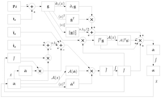
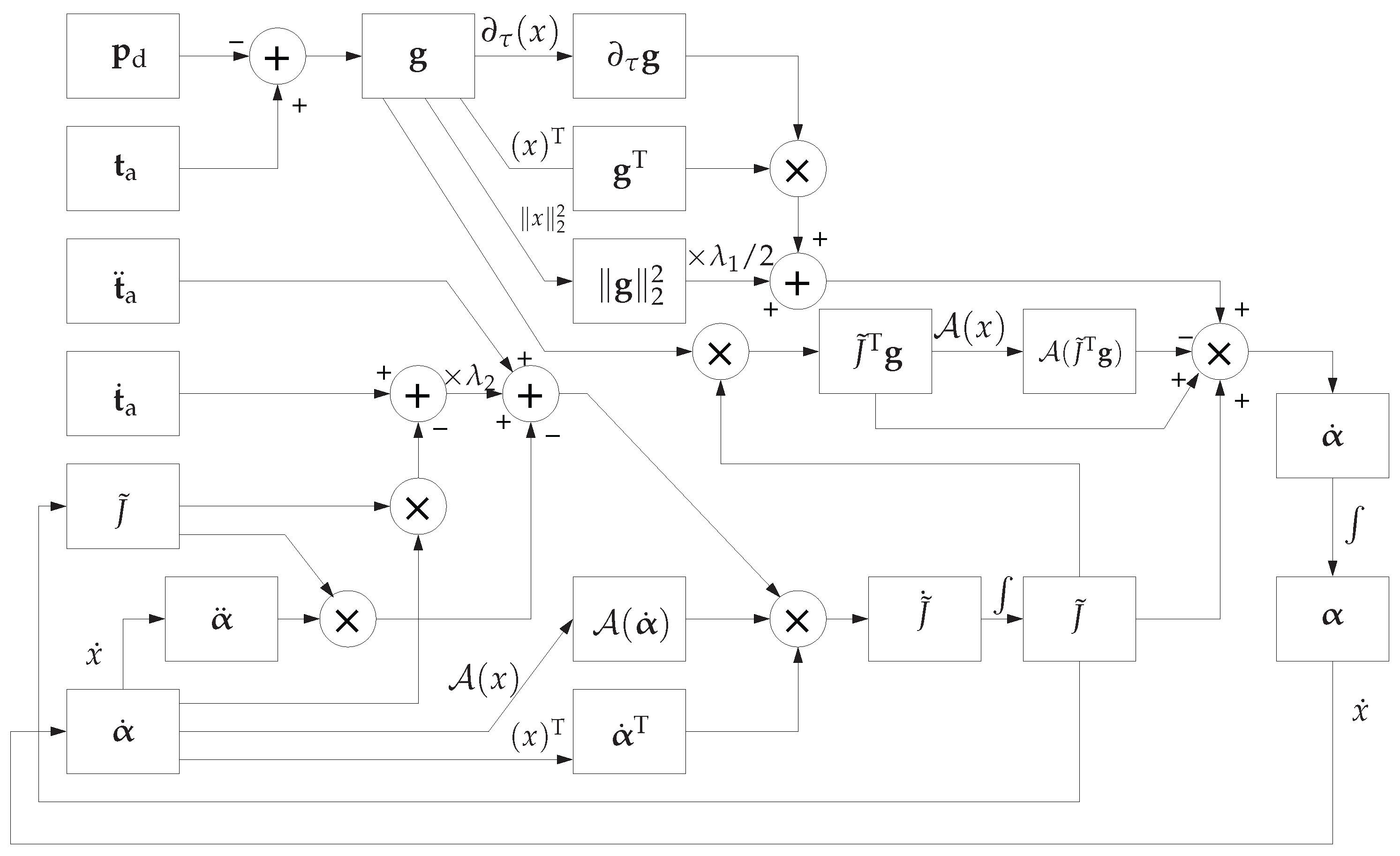
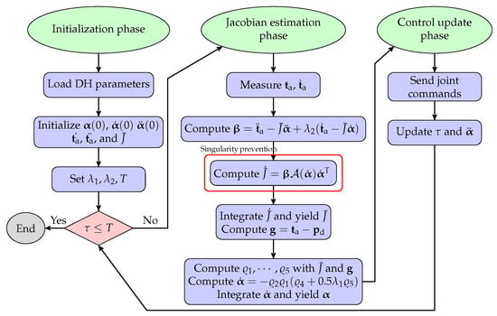
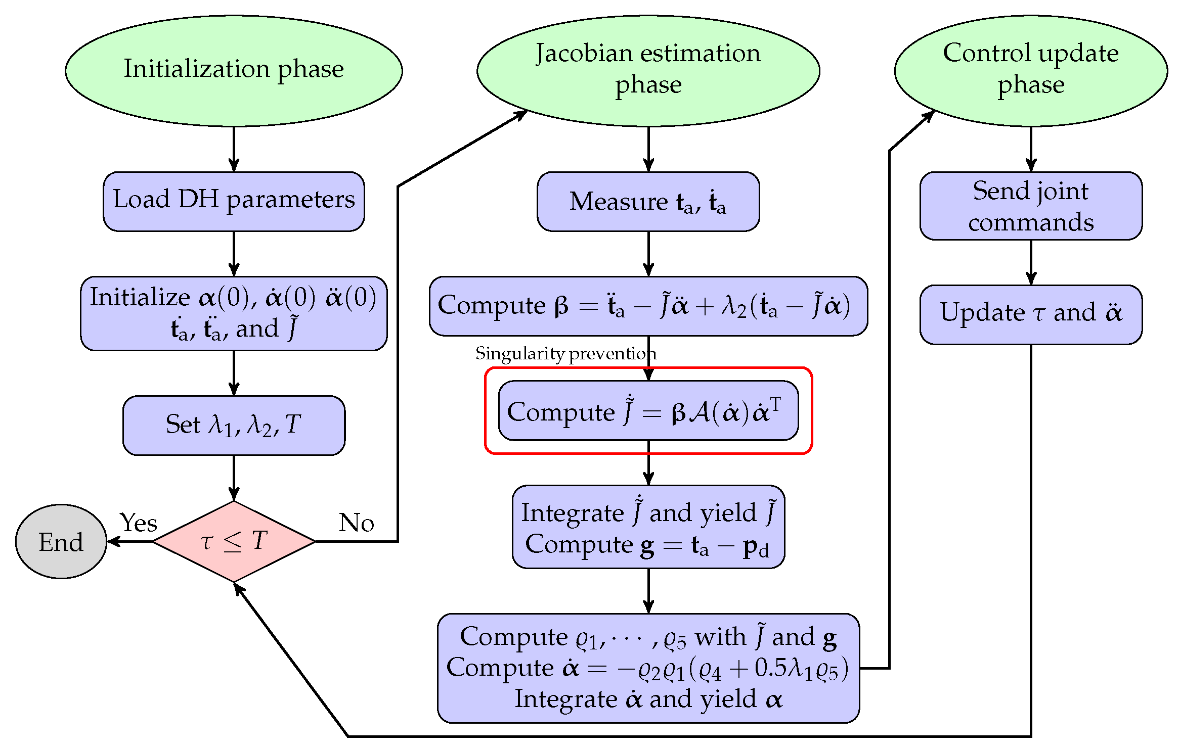
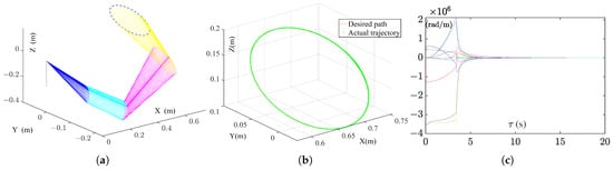
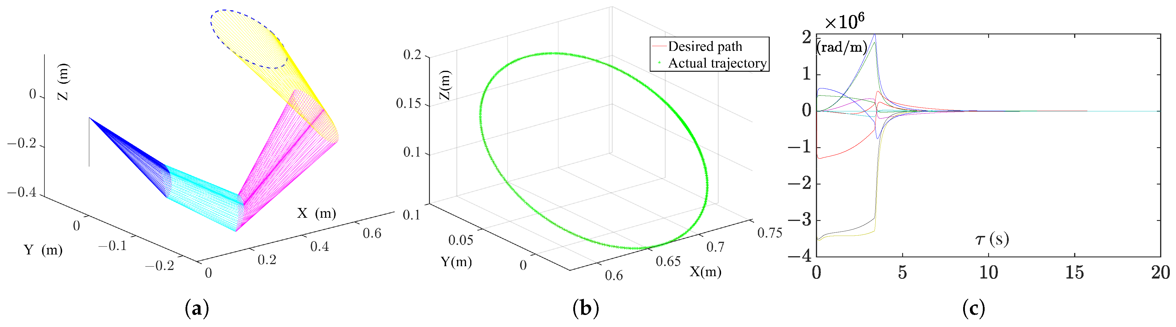
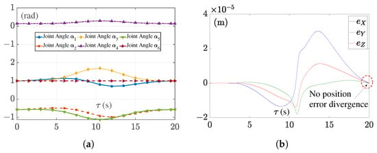
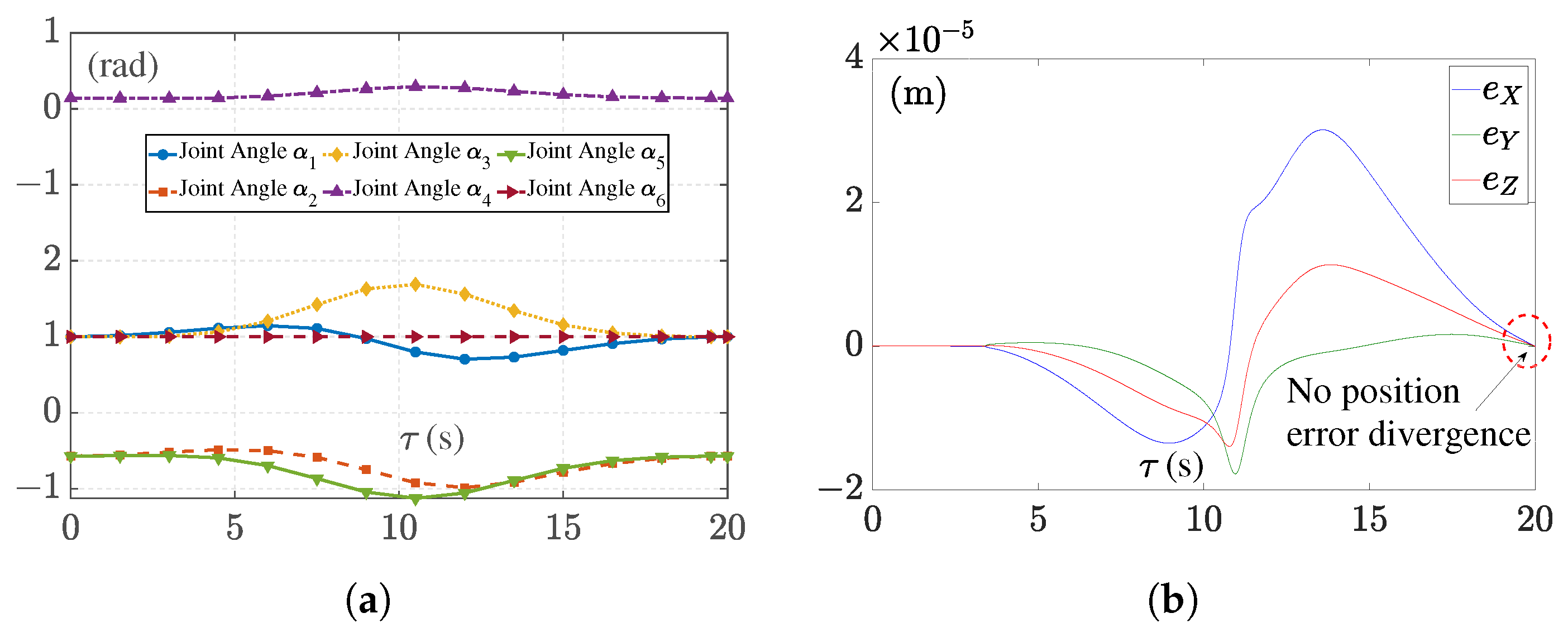
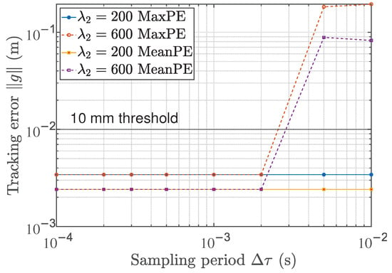
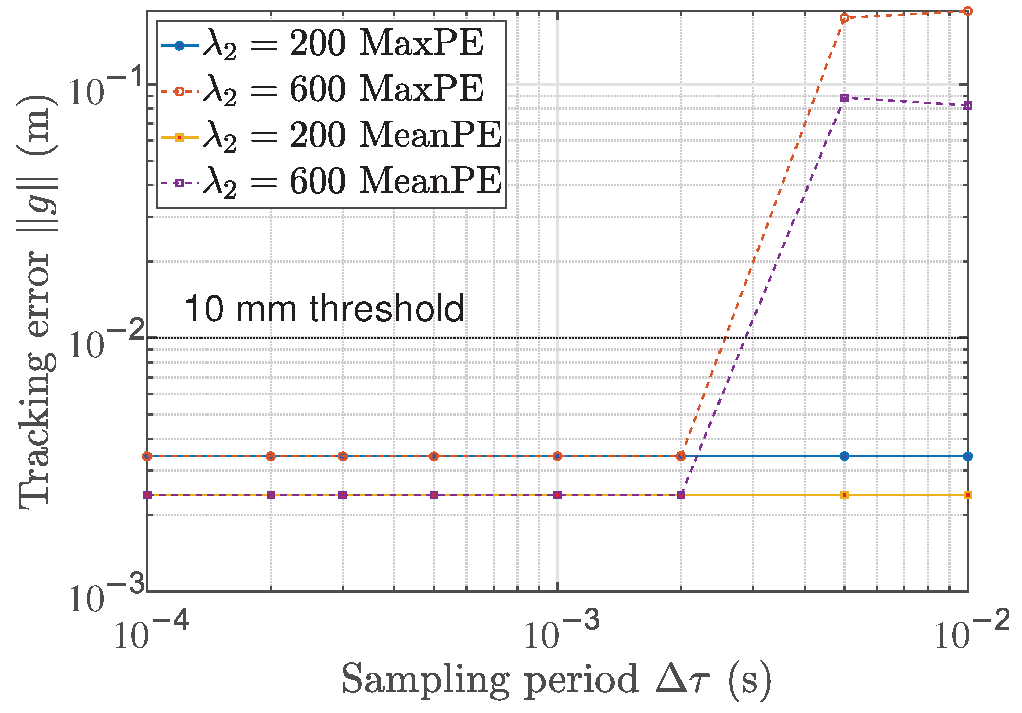
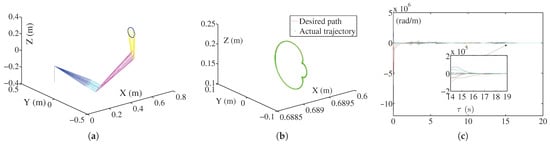
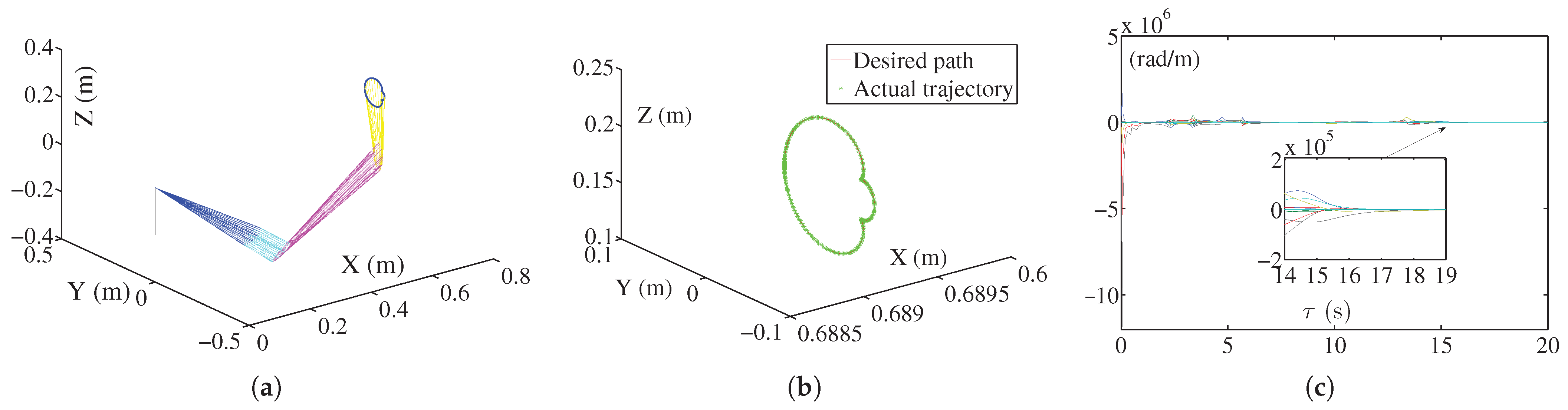
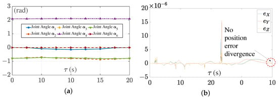
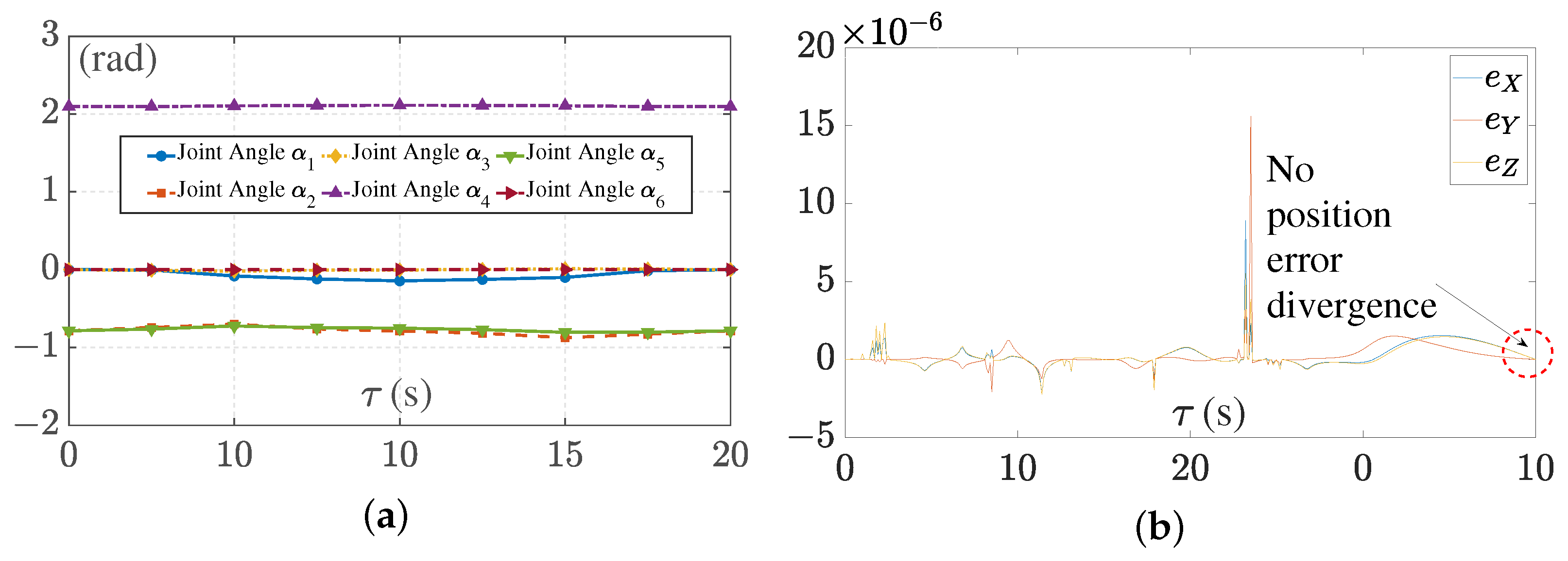
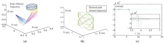
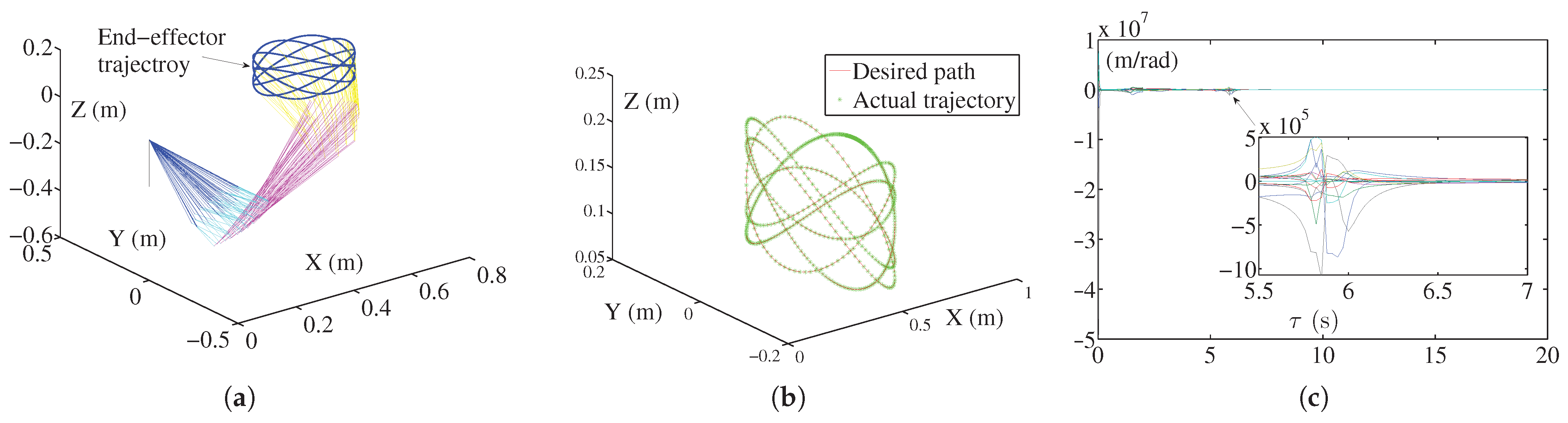
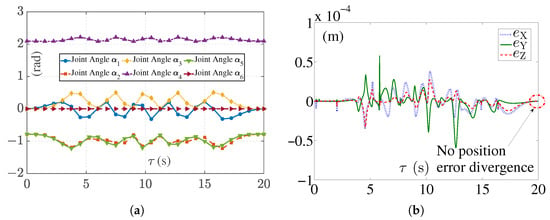
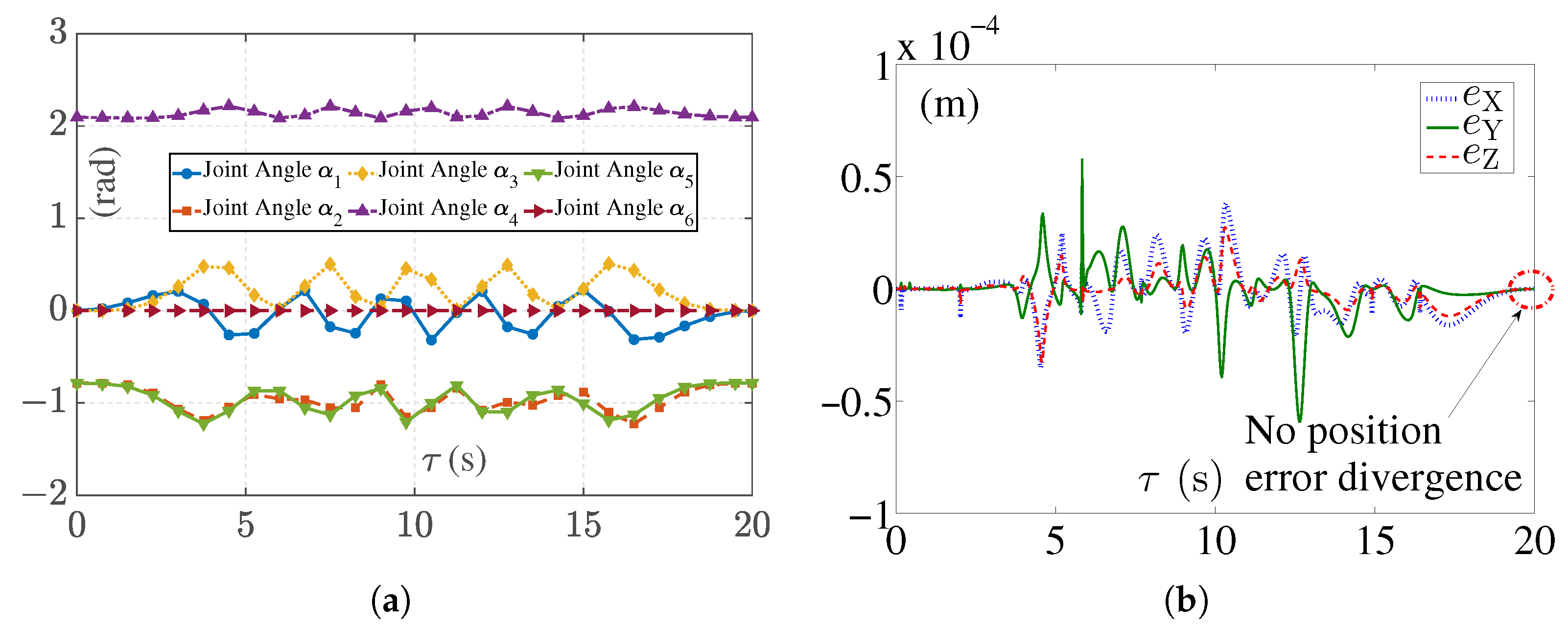
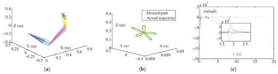
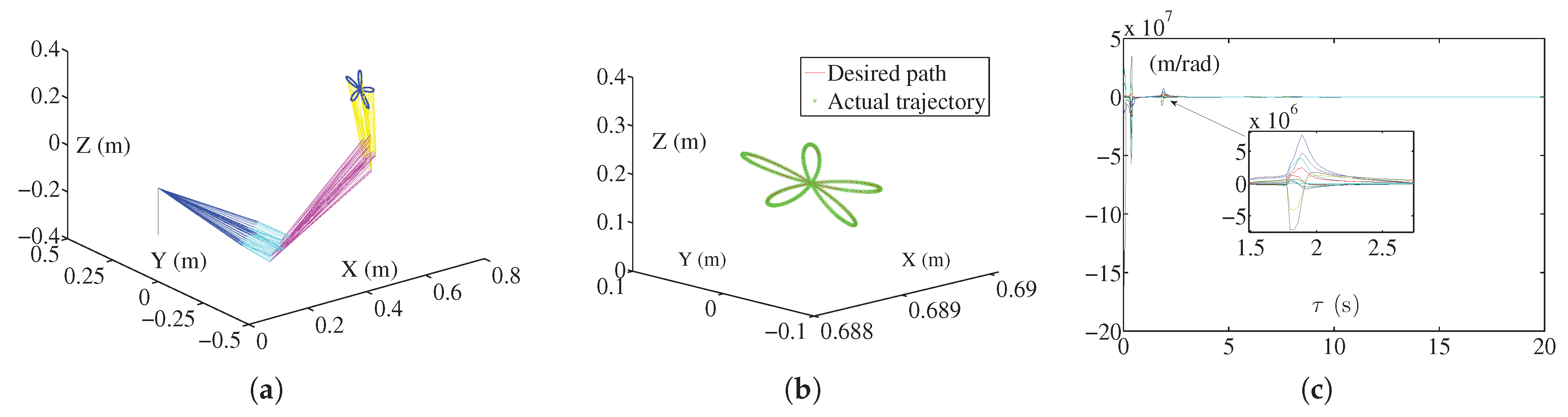
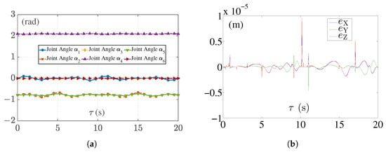
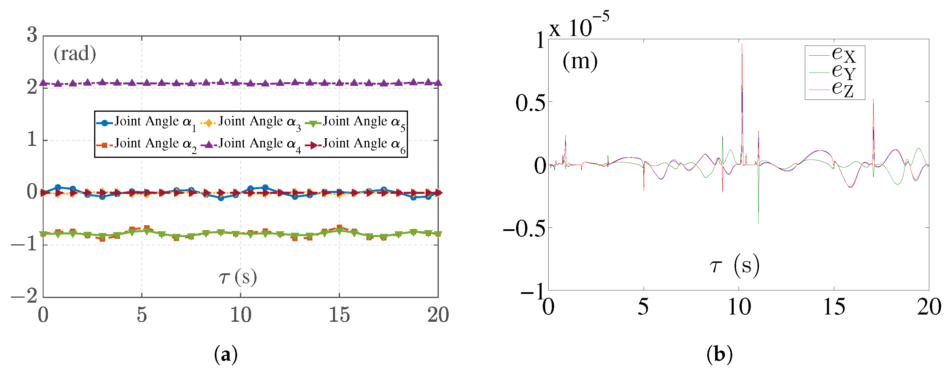
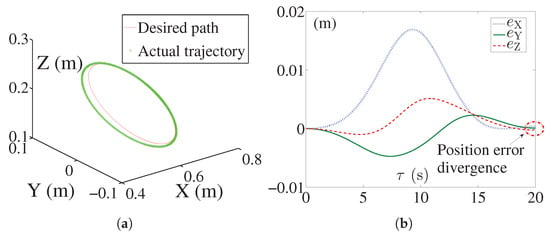
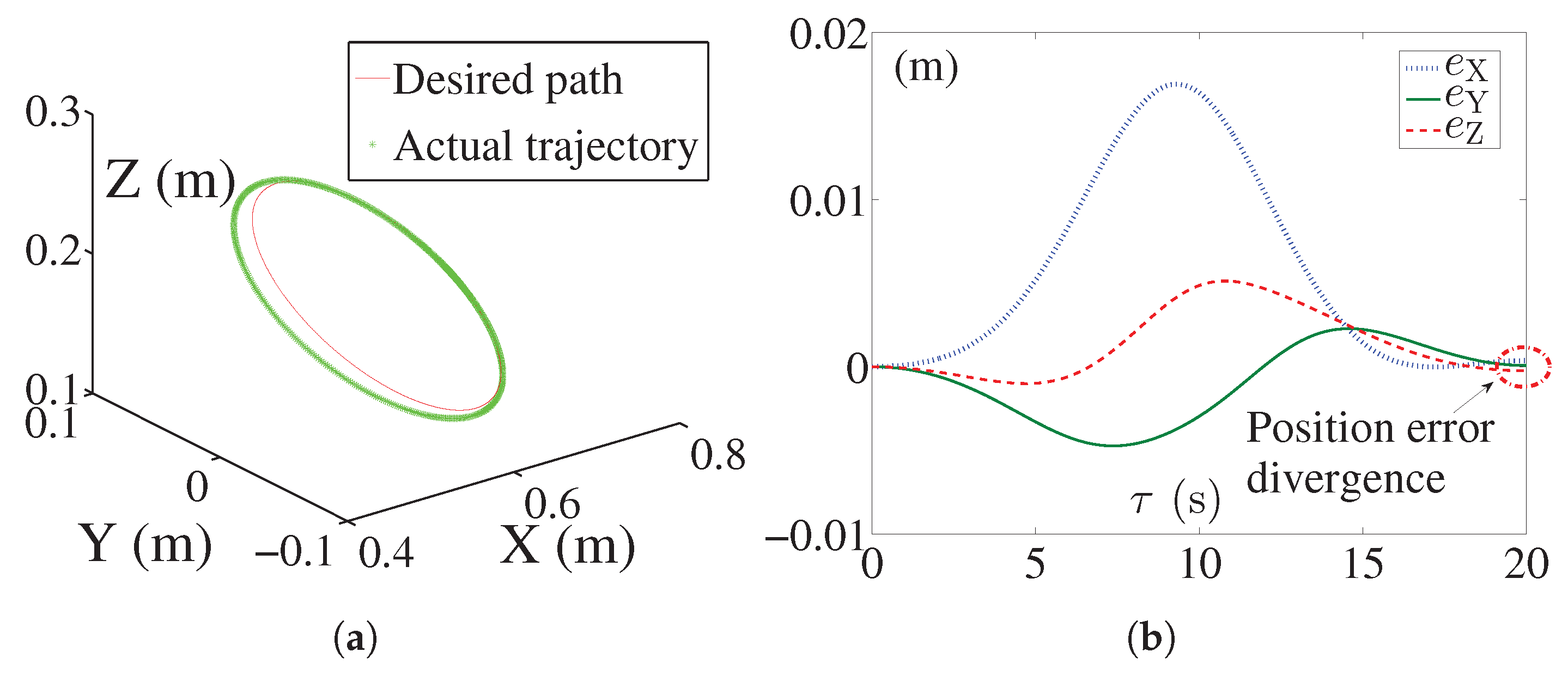
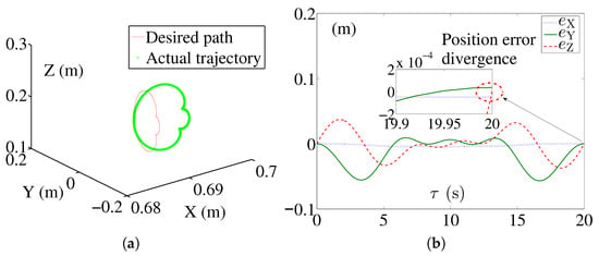
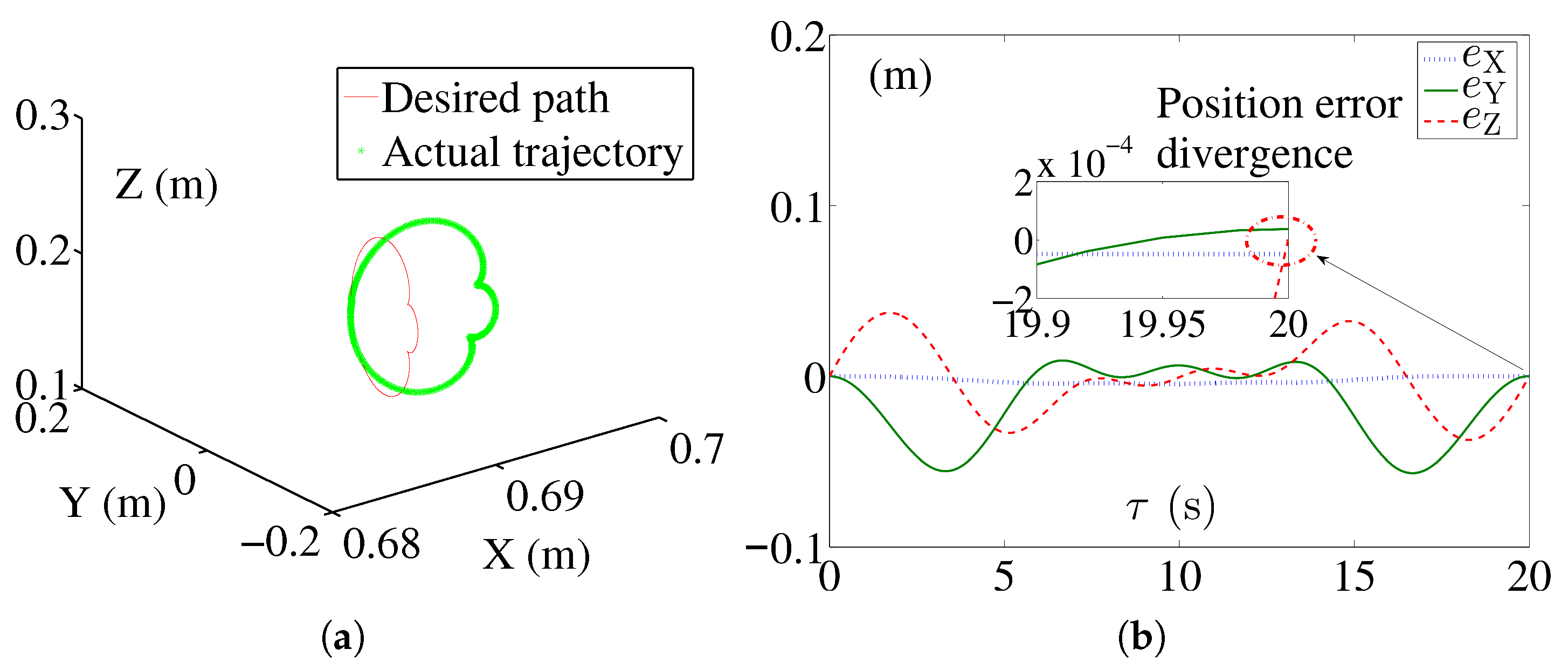
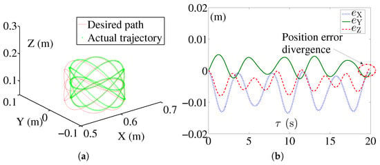
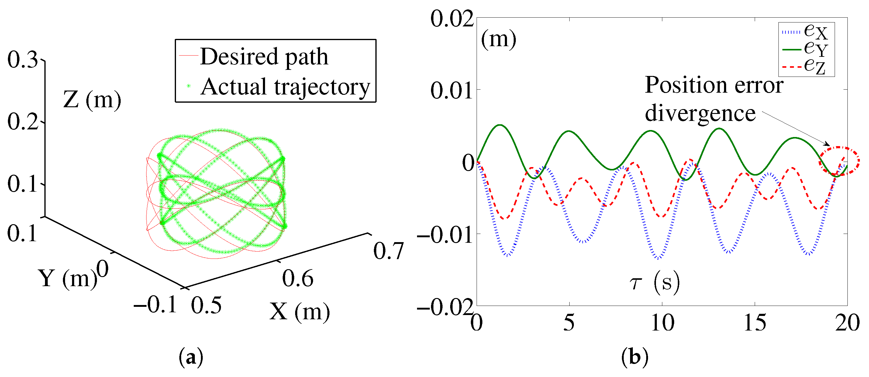
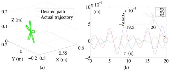
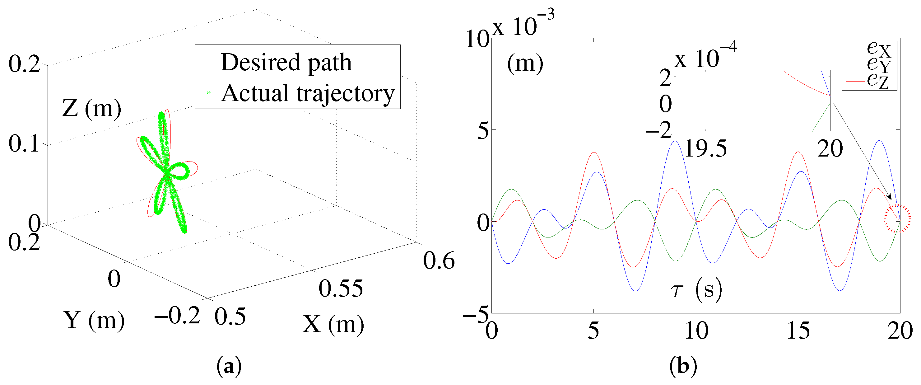
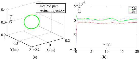
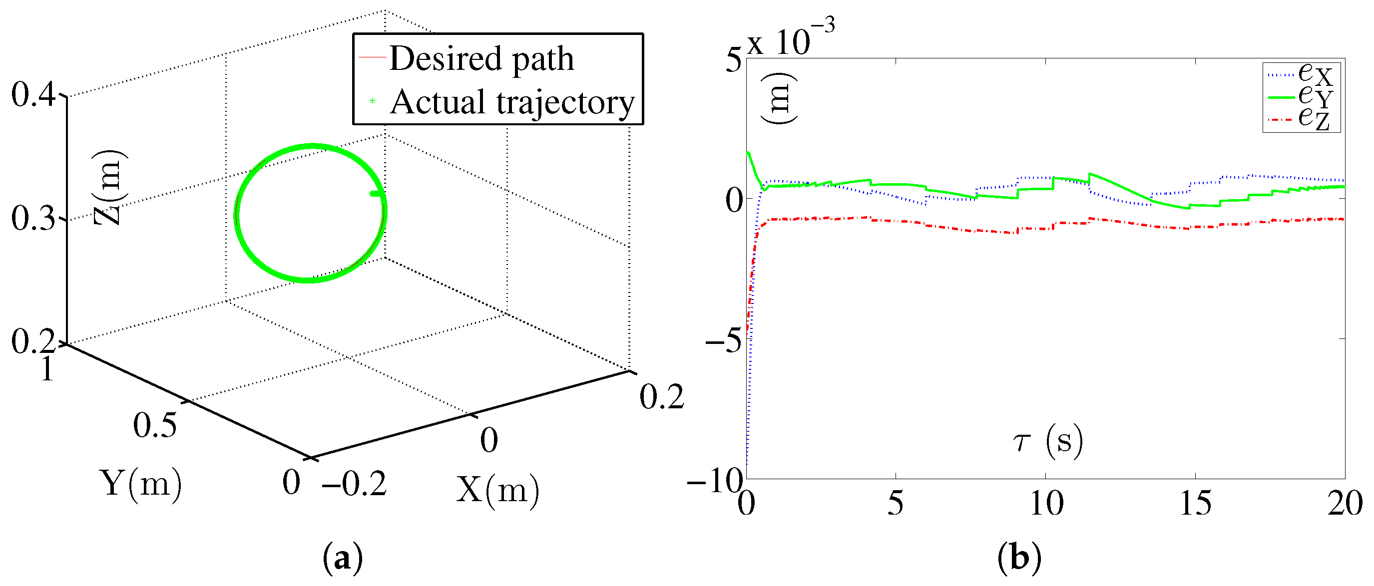
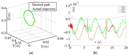
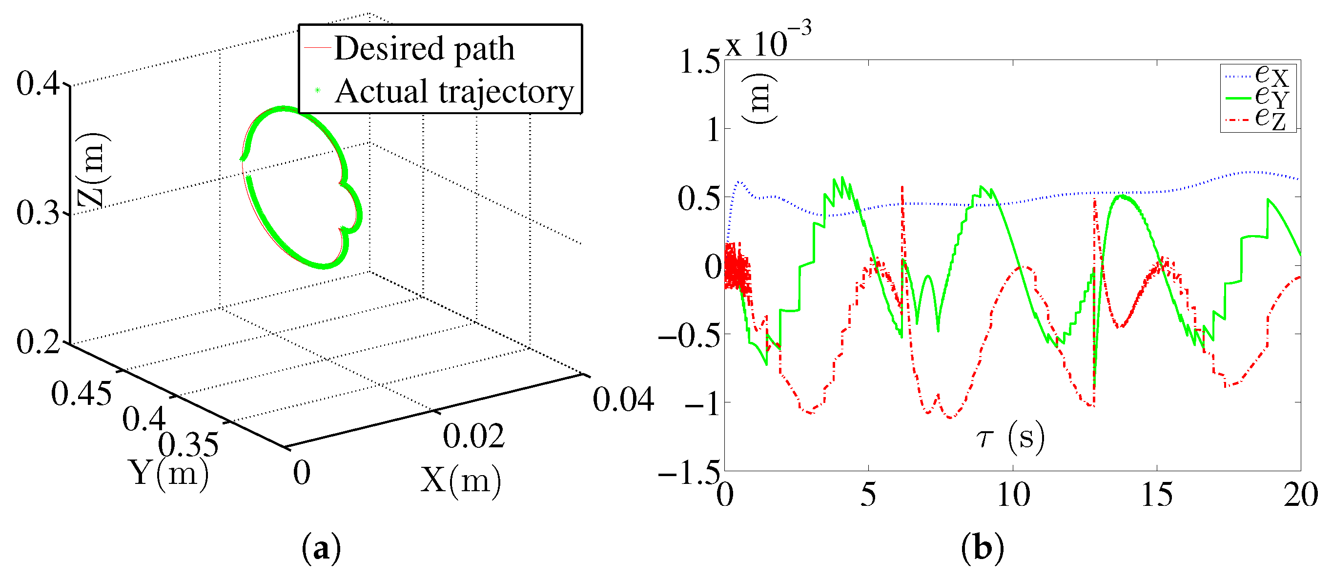
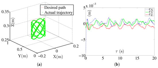
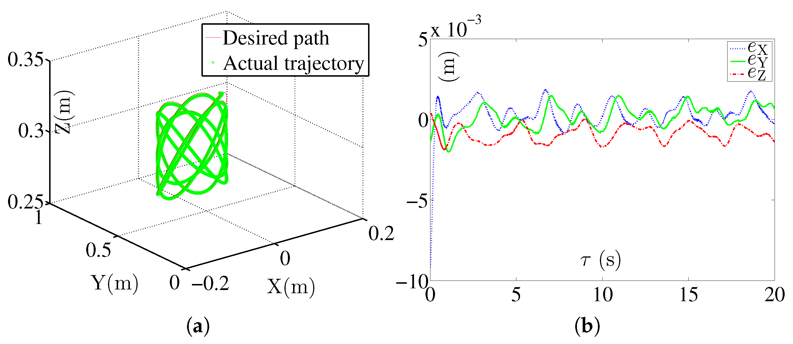
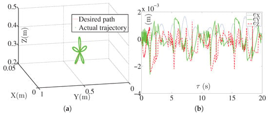
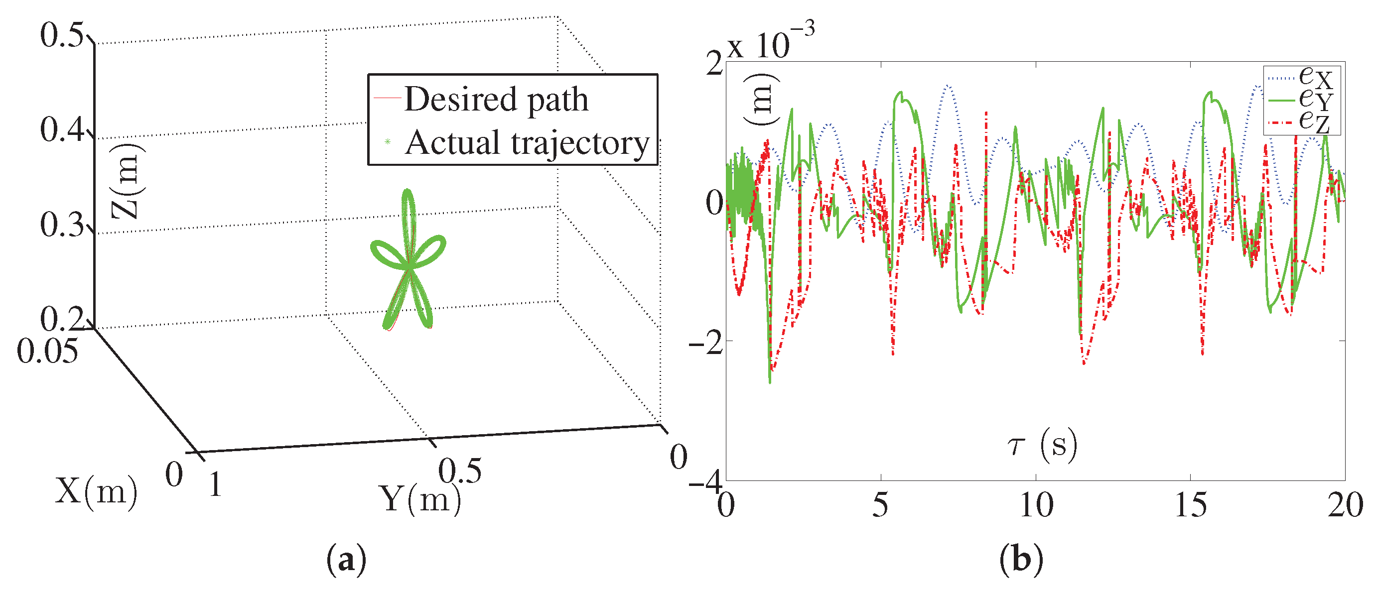
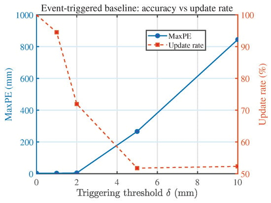
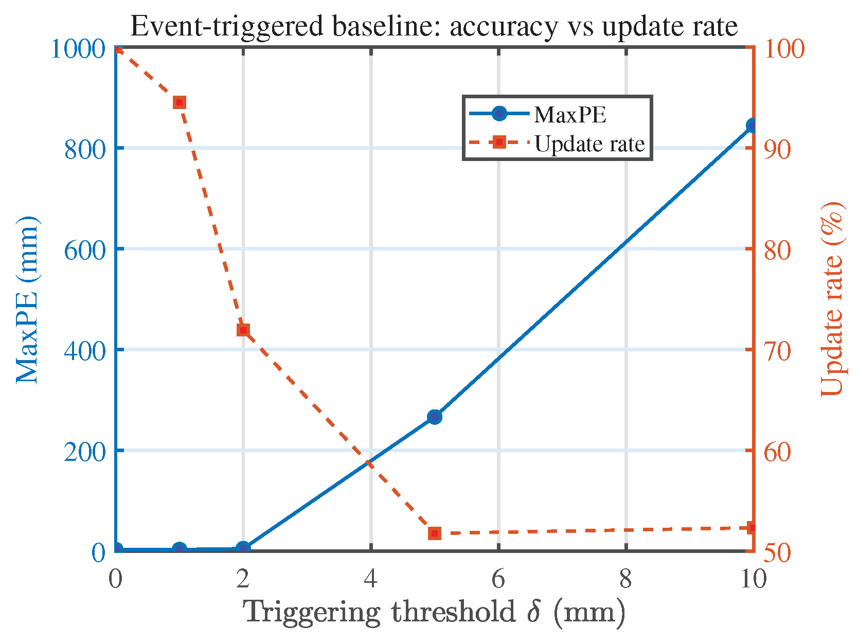
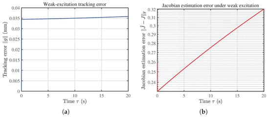
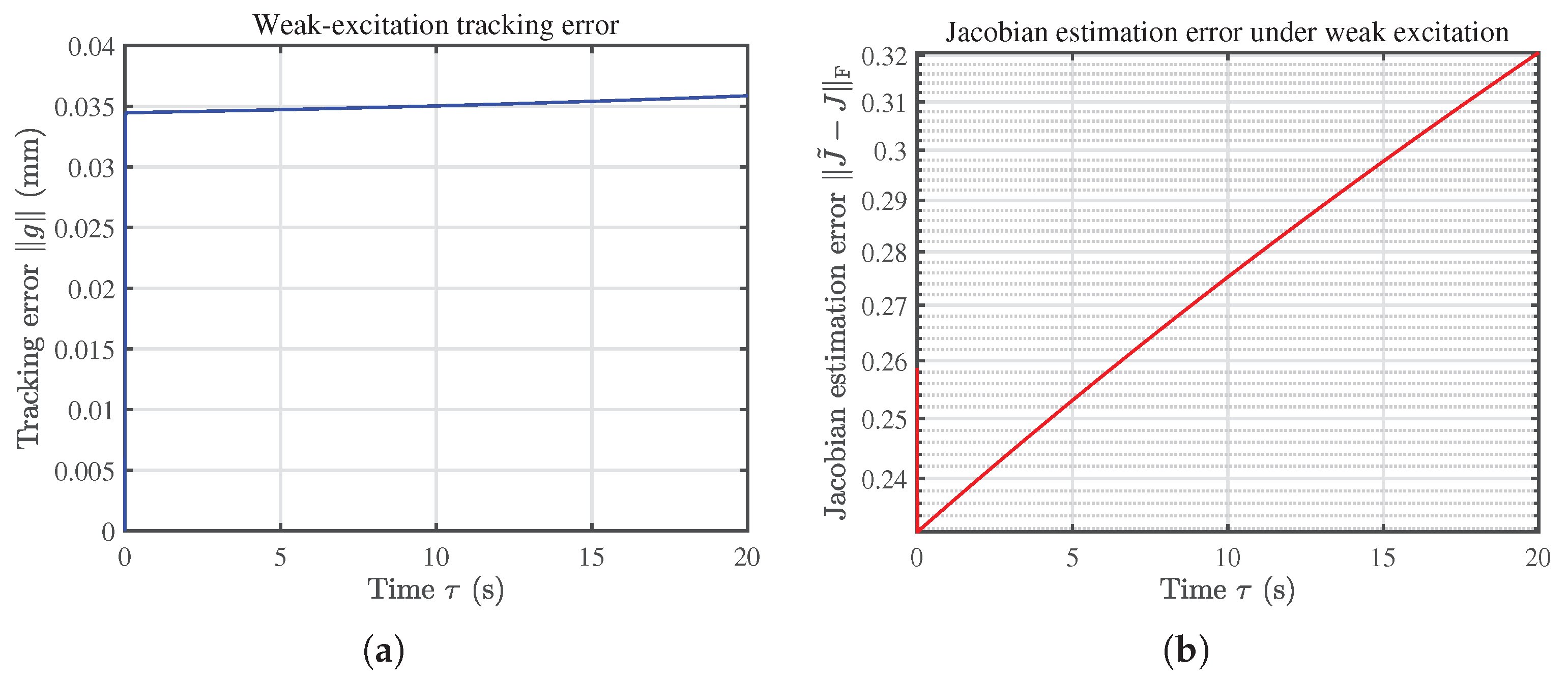
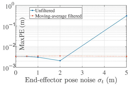
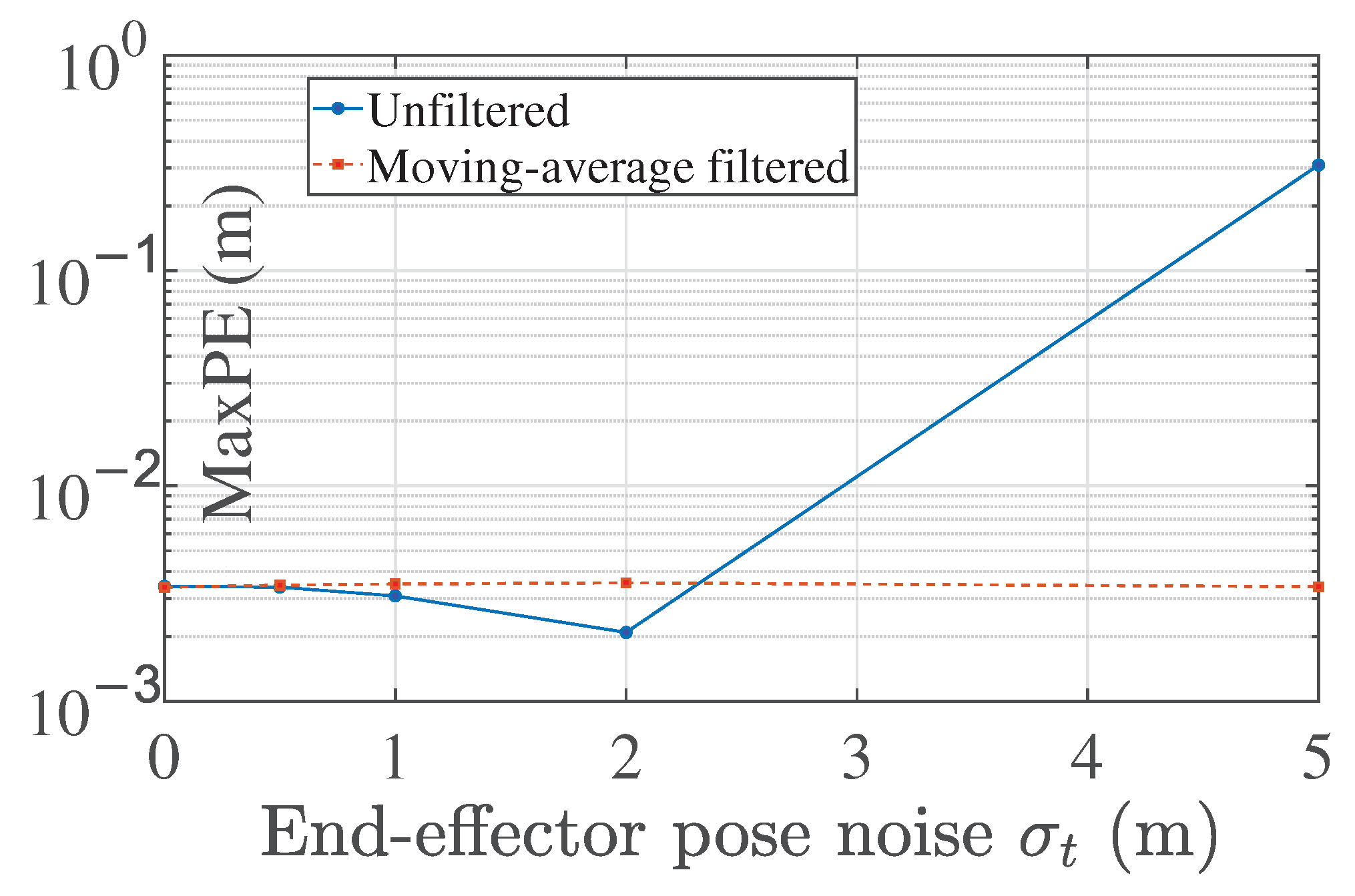
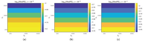
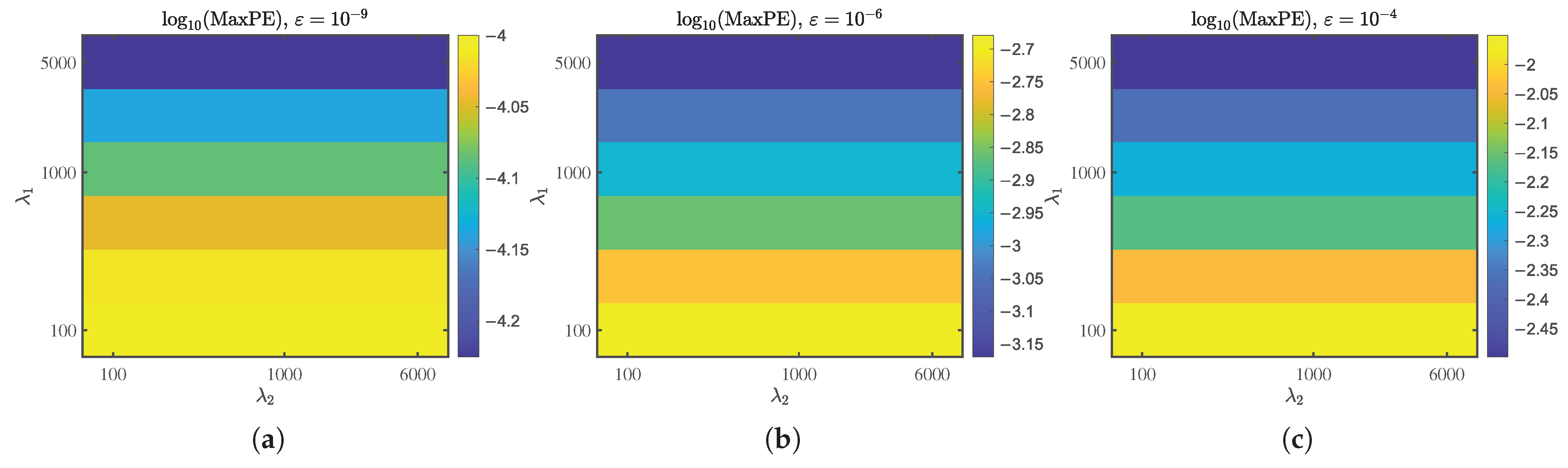
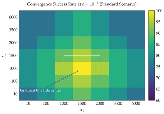
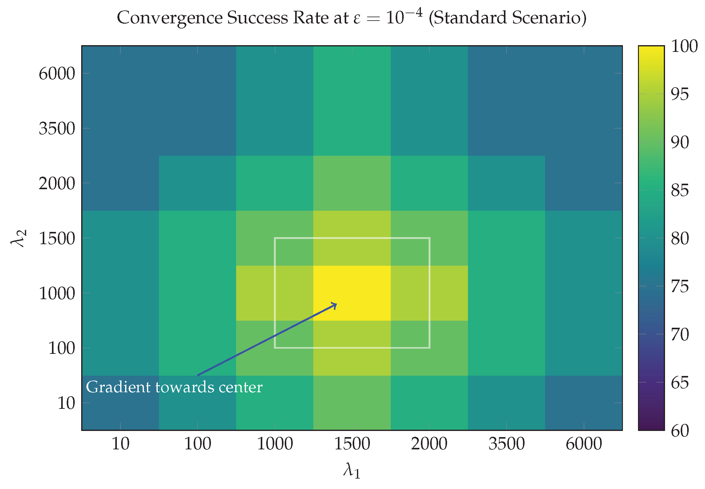
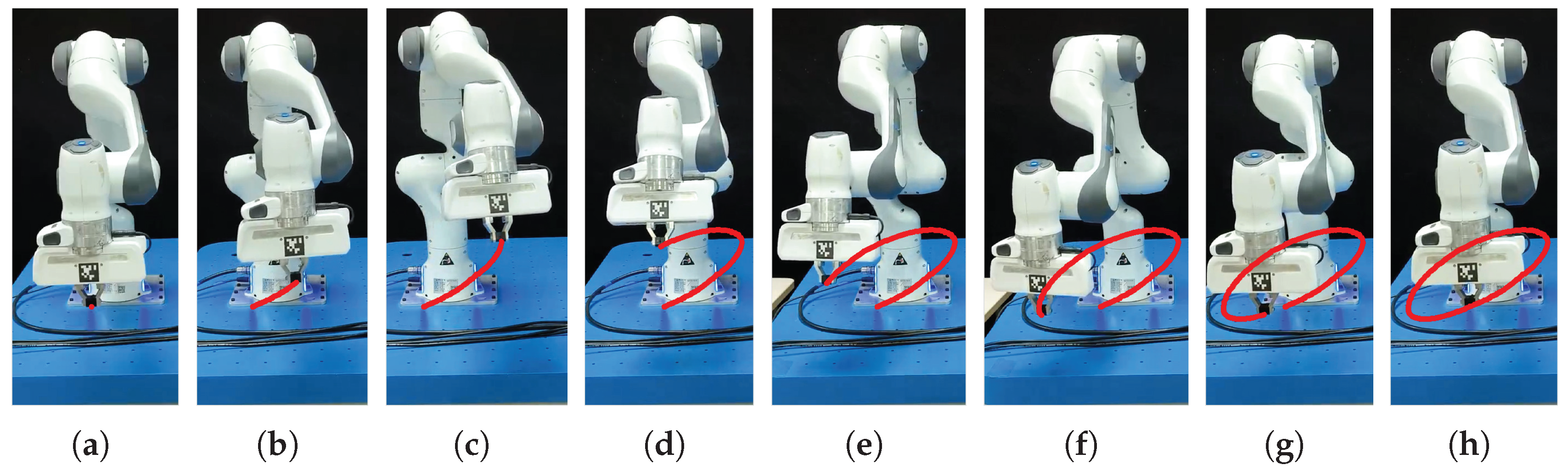
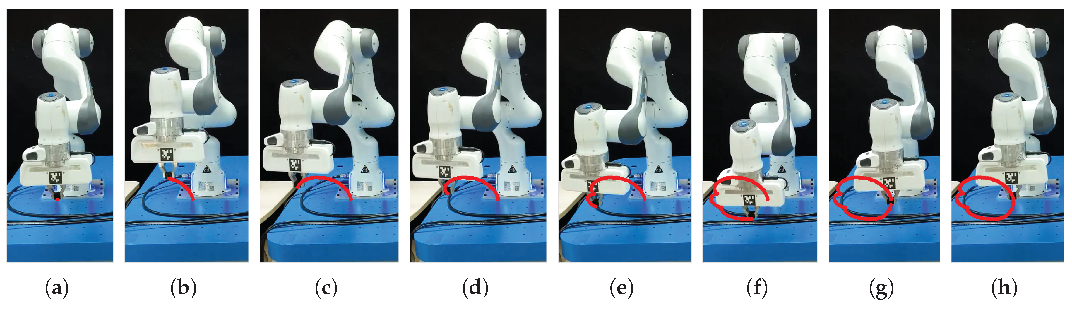


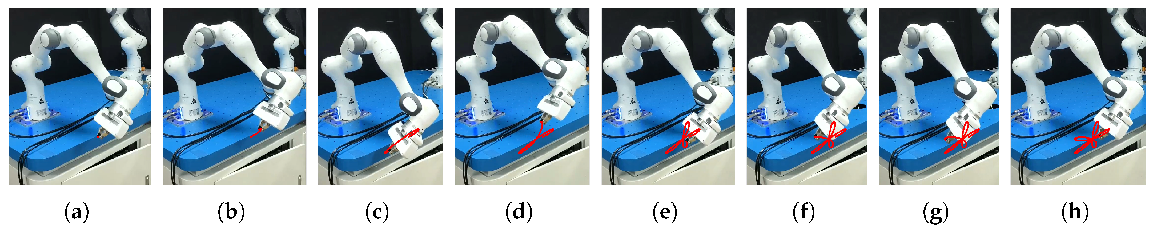

Disclaimer/Publisher’s Note: The statements, opinions and data contained in all publications are solely those of the individual author(s) and contributor(s) and not of MDPI and/or the editor(s). MDPI and/or the editor(s) disclaim responsibility for any injury to people or property resulting from any ideas, methods, instructions or products referred to in the content. |
© 2026 by the authors. Licensee MDPI, Basel, Switzerland. This article is an open access article distributed under the terms and conditions of the Creative Commons Attribution (CC BY) license.