


Abstract
Evaluating water quality is fundamental to ensuring that freshwater ecosystems support the well-being of all life on Earth. The present study uses physicochemical parameters to assess groundwater in Dili, Timor-Leste, from 2011 to 2018. Water quality was determined using the conventional Water Quality Index (WQI), aggregated via a weighted sum function aligned with the World Health Organization (WHO). The study aims to predict the WQI and water quality status, expressed as Water Quality Classification (WQC), to support sustainable water resource management. In low-resource domains, it is crucial to address challenges related to small dataset size and class imbalance in the sample observations. However, deep learning models are highly dependent on the availability and quality of training data. This paper builds upon prior data augmentation strategies for water quality data analysis, aiming to overcome the constraints of a small dataset in predicting the WQI and WQC. To address these issues, the study extends prior data augmentation strategies and introduces WQ-ERT (Water Quality Encoder Representations from Transformer). This Transformer-based model applies Gaussian noise augmentation and a class-balancing strategy. The model has been pre-trained on a large Indian water quality dataset with similar soil-type characteristics and fine-tuned on the Timor-Leste water quality dataset, using a Gaussian noise value of = 0.20 for the Indian datasets, whereas for Timor-Leste, it uses a lower Gaussian noise value of = 0.05. Furthermore, to address label imbalance in the classification target, a random search-based class-balancing technique is employed during fine-tuning. We conducted six experiments to evaluate our proposed model and applied five-fold cross-validation. The results demonstrate that noise augmentation substantially improves WQC performance, achieving 97.0% balanced accuracy, and WQI prediction reaches an R2 of 0.703, indicating better generalization across the dataset. Class-balancing techniques enhance WQC, particularly in balanced accuracy, F1-score, and the Matthews Correlation Coefficient (MCC). This configuration reduces false negatives by 86.05% for water quality classification, though excessive weighting slightly lowers precision. In WQI prediction, the experiment shows a 7.92% reduction in MAE, improving few-shot adaptation to Timor-Leste without distortion.
1. Introduction
Monitoring Water Quality (WQ) poses a significant global challenge, particularly in low- and middle-income countries. Insufficient daily monitoring in these regions hinders hotspot and trend identification because of data shortages [1,2]. Capacity and development-level challenges, including human resources and financial and technical capabilities, increase significantly in countries with lower human development across all stages of monitoring, including institutions, parameter selection, and field analyst skills [3]. Many water sector agencies and local communities often rely on irregular sampling and manual assessment, which are often slow, costly, prone to data gaps, and unable to capture rapid changes in water conditions [4,5,6]. The examination of water quality is important for ensuring the suitability and integrity of the water environment for diverse uses, including human consumption, agriculture, tourism, health, industry, and the ecological environment. Recent research has focused on developing machine learning and deep learning models to predict water quality. These models rely on extracting temporal features and incorporating multiple factors [7,8]. A Long Short-Term Memory (LSTM) model is employed to perform medium- to long-term water forecasts of drinking water quality and river parameters, where LSTM learns time-dependent patterns in complex, non-stationary water quality data [9,10,11]. The integration of attention mechanisms in deep learning with LSTM (AT-LSTM, FTA-LSTM) has been demonstrated to enhance the forecasting and detection of anomalous shocks, surpassing the performance of plain LSTM and a Transformer-like multi-layer perceptron (MLP) encoder with WWTP data [12,13].
Several studies have employed artificial neural networks and other neural network-based methods to predict the WQI and WQC from physicochemical variables. In groundwater classification, ANN accuracy was 66.67% with 17 parameters, 83.33% with five parameters, and 91.67% with chromium alone [14]. Similarly, in coastal China, ANN predicted WQI grades at about 93% accuracy, while RF and other tree-based models exceeded 95% [15]. An MLP study for WQC in Pakistan achieved 85.07% accuracy using only four parameters, emphasizing low-cost real-time feasibility over maximum performance [16]. For example, for the WQI in the Warta River study, ANN predicted surface-water WQI from five inputs with R = 0.9792 and = 0.6245, while reducing the required variables from 11 to 5 [17]. A Tekanpur study reported about 93% predictive precision for a back-propagation feed-forward ANN estimating the WQI from forty physicochemical variables, which is clearly below the highest values reported elsewhere [18]. In the Shivganga basin groundwater, a three-layer back-propagation ANN trained with Levenberg–Marquardt performed satisfactorily across seasons but suffered from overfitting [19]. While this approach demonstrates the power of neural networks for WQI prediction and WQC, it often faces limitations such as overfitting, class imbalance, and difficulty capturing complex feature interactions, especially with limited data and noisy values. To address these limitations, this study is inspired by the Transformer model, which aims to provide greater robustness, improved accuracy, and enhanced interpretability for WQI prediction.
Advances in Natural Language Processing (NLP) and its application to structured data have led to the adoption of the Transformer architecture. Transformer and attention-based models have emerged as state-of-the-art and were introduced for modeling longer sequences in language translation [20]. This model has been implemented for several tasks, including time-series data prediction [21,22], with the most success in structured health records and multimodal time-series, where masking data and adopting an attention mechanism capture complex dependencies [23]. A Transformer-based WQ time-series model (DPSGT) uses decomposition and patching to learn trends and fluctuations, and it improves performance metrics such as Root Mean Square Error (RMSE) and Mean Absolute Error (MAE) compared to another model [24]. A multistep watershed model combines Savitzky-Golay denoising with a Transformer-optimized network and a time-series-aware DILATE loss to reduce noise and lag in multi-step forecasting [25].
According to a previous study, the Transformer has been applied to tabular and sequence-based learning models (ALBERT-WPD), achieving 95% accuracy in predicting water suitability for agricultural purposes with fewer parameters than traditional models [26]. While sparse-attention Transformer models effectively classify aquaculture water quality, integrating with real-time data achieves 99.79% accuracy and enables proactive management of fish and aquatic organisms. For example, K. Roteiro et al. [27] achieved an accuracy of 91.4%, while K. Sunil et al. [28] reached 94.5% using a tab-Transformer with IoT sensor data. Our previous study leveraged a Transformer encoder architecture within a cross-regional learning strategy, achieving 96.62% accuracy. Transfer learning can address the problem of limited data in target regions by pre-training a deep learning model on a rich source-domain dataset and fine-tuning it on a portion of the target-domain dataset [29,30]. One such architecture is a model that classifies water quality status and predicts the Water Quality Index (WQI). This model uses the Bidirectional Encoder Representations from Transformers (BERT) and employs a masking approach to mitigate biases and inaccuracies commonly associated with conventional imputation methods. Water quality features used to determine the WQI and for water suitability analysis play a role in water management. These features help decision-makers and companies ensure clean, suitable water for communities and other essential needs. This system also serves as an early warning mechanism for detecting water contamination within the country.
Although using two datasets to improve the generalizability of the Transformer-based model has been shown to improve robustness to noisy test data, adding Gaussian noise to image, time-series, or tabular inputs improves robustness to noisy test data; however, applying it globally may reduce accuracy on clean data. For material sample generation, Multi-Distribution Mega-Trend Diffusion (MD-MTD), Generative Adversarial Network (GAN), and t-SNE are combined with Gaussian process regression, markedly improving groundwater quality prediction when data are scarce [31]. Adding Gaussian noise to material data improves the efficiency and accuracy of the machine learning model in predicting high-entropy alloy phase and hardness [32]. Data augmentation techniques can effectively increase the size and consistency of time-series datasets, thereby improving deep learning performance in the field [33]. The integration of Gaussian noise into image, time-series, or tabular data inputs improves robustness against noisy test data; nevertheless, it may adversely affect accuracy on clean data when applied globally [34]. Therefore, the source-domain dataset is expected to support model training in the absence of large-scale labeled data in target regions [35]. To mitigate data scarcity, missing values, and class imbalance, we employ a synthetic data generation approach that expands the dataset while preserving privacy.
In this study, we propose a unified framework that combines cross-regional learning, a Transformer-based encoder, and Gaussian noise augmentation to enhance water quality prediction in Timor-Leste. Our contributions are threefold. First, we demonstrate that leveraging a larger, heterogeneous dataset from another country can substantially improve model performance in Timor-Leste, where labeled data are scarce. Second, we show that integrating noise augmentation and class-balancing strategies strengthens water quality classification by improving robustness and mitigating data imbalance. Finally, we provide a comprehensive evaluation across multiple experiment configurations, revealing that a combined noise-augmented and balanced approach yields the highest accuracy, generalization, and stability.
Recently, researchers have made exciting strides in applying deep learning methods to water quality models, and the results are undeniable. However, significant gaps remain, particularly in the framework of Transformer-based models and their use for structured water quality datasets: (a) Limited use of Transformer models for tabular water quality datasets, with most research focusing on time-series or spatiotemporal data. This use in environmental science remains underexplored. (b) Lack of studies evaluating Transformers using data from low-resource countries like Timor-Leste, limiting model generalizability. (c) Few studies have applied fine-tuning strategies for cross-region adaptation and improving model interpretability in the water quality context. This research aims to predict the WQI and water suitability in Timor-Leste, mainly using physicochemical parameters.
2. Datasets
2.1. Study Area
This study focuses on Dili City, Timor-Leste, as the target for our main region (Figure 1a). Additionally, we trained the model using an online Indian water quality dataset, which served as the source domain for seven states (Figure 1b).The blue frames indicate the study areas of the water quality data collection. In Timor-Leste, the blue frame highlights Dili. In India, the blue frames indicate the states from which water quality data were collected, namely Tamil Nadu, Andhra Pradesh, Maharashtra, Gujarat, Bihar, Assam, and Uttar Pradesh.
Figure 1.
Study areas of two regions: (a) Mapping of water quality sampling points in Dili, Timor-Leste. (b) Mapping of water quality sampling points in the Indian water quality dataset.
We selected a source-domain sample with similar soil-type properties to ensure cross-regional comparisons are technically valid and not influenced by ecological disparities. For the Indian dataset, we use water samples from the six blue states in Figure 1b. For the Timor-Leste dataset, we select eight water sampling points in Dili. The Euclidean distance is applied to measure distance in clustering, nearest neighbors, and vector-space models; two objects are treated as similar when their distance is closer to 0 [36,37] in the case of the Timor-Leste and Indian datasets to quantify the similarity of the soil types. Given that both areas are predominantly located in coastal zones, where soil formation processes and sedimentary characteristics are comparable, the analysis focused on soil-type analogs of the Timor-Leste dataset found, namely, Fluvents, Usterts, and Ochrepts [38]. In India, analogous soils include coastal black soil (Regur), red soil, laterite soil, and alluvial soil [39,40]. This alignment is pivotal in ensuring the coherence, environmental reliability, and environmental consistency of subsequent modeling and interpretation.
In selecting samples, we used eight standardized water quality features for all samples and soil type (encoded) for every sample. For samples in the Indian dataset, if the soil type matched that of the Timor-Leste water samples, it automatically selected the Indian sample for further analysis. If the soil did not match, we applied k-nearest neighbors (k = 15) using Euclidean distance in the feature space to identify the most similar Indian samples to those from the Timor-Leste sample. This two-step procedure ensures that, whenever possible, we prioritize soil-type similarity; otherwise, we rely on empirical proximity in the standardized feature space to select representative samples. These low distances indicate that, for each Timor-Leste sample, closely matching Indian samples exist in multidimensional space. The substantial overlap between the two datasets demonstrates a high degree of similarity, supporting the use of transfer learning from the Indian dataset to the Timor-Leste dataset, as illustrated in Figure 2.
Figure 2.
Optimized UMAP projection of standardized water and soil features for samples from India (blue) and Timor-Leste (orange).
2.2. Dataset Description and Descriptive Analysis
The dataset we used in this study consists of two Indian water quality datasets and the Timor-Leste water quality dataset. The deep learning models in this study are trained on a publicly available dataset on GitHub, repository in CSV file and the Indian water quality dataset [41]. The dataset contains 19,029 samples collected from multiple states and districts between 2019 and 2022. Each record includes a unique well ID, location details (state, district, block, village), latitude and longitude, and sampling year.
Although the full dataset contains sixteen features, we use only eight features because they match the parameters of Timor-Leste water quality: pH, Total Dissolved Solids , Total Hardness , Electrical Conductivity EC (μS/cm), calcium , nitrate , sulfate , and fluoride were selected to evaluate drinking Water suitability using the WQI based on permissible limits defined in WHO guidelines for drinking water quality [42,43]. Each water sample has a quality status, such as suitable or unsuitable for human consumption. Considering different conditions, geographically and infrastructurally, we select 8941 samples based on a similar soil type. Secondly, the Timor-Leste water quality dataset is employed as a testing dataset, with 2161 samples, which is obtained from the national laboratory of water quality monitoring in Timor-Leste of the Ministry of Public Works.
The Timor-Leste dataset contains 77 missing entries, corresponding to 3.5% missing values due to irregular sampling, no water flow, and unexpected events such as logistical issues, instrument failure, and heavy rain. Missing values in the Timor-Leste dataset occur at different rates across parameters, but the pattern is predominantly Missing At Random (MAR) because missing values are not concentrated at specific sampling points, indicating that missingness stems from routine measurement gaps rather than spatial or temporal bias. Table 1 below shows additional information on missing values for all parameters in this study.
Table 1.
Missing values in the Timor-Leste water quality dataset.
To address missing data, we employ model-based imputation techniques, including KNN or median imputation, or replace them with the mean prior to calculating the WQI [44]. In our previous study, missing values were not imputed; instead, parameters with missing observations were excluded from the WQI calculation, which was performed using only the available data for each sample. In addition, the model was trained directly on the MASK token to represent missing values [29]. To evaluate the robustness of the model, we trained the same dataset containing missing values in the present study. This dataset was trained by applying data augmentation and class balancing for this purpose.
The normalized distributions of water quality parameters such as pH, EC, F, NO3, TH, Ca, and TDS show broadly similar patterns for both India and Timor-Leste, with most values concentrated at the lower end and right-skewed shapes. Indian water quality generally exhibits a wider range and more extreme values for most parameters, while Timor-Leste distributions are tighter with occasional outliers, especially for fluoride and calcium. Overall, these comparisons indicate substantial overlap, supporting the suitability of using the Indian dataset as a source domain while also highlighting regional differences, illustrated below in Figure 3 and Figure 4.
Figure 3.
Distribution of normalized water quality features of the Indian dataset.
Figure 4.
Distribution of normalized water quality features of the Timor-Leste dataset.
The Water Quality Index (WQI) is a critical metric for assessing the suitability of water supply for all human use and must be accurately predicted to ensure the sustainability of water resources [45]. In this study, the WQI is calculated by averaging the individual indices of some or all parameters [46,47]. We used physicochemical parameters to compute the WQI through the weighted arithmetic index method, and we applied the scores to classify groundwater quality in Dili, Timor-Leste. The WQI is calculated as
where N denotes the total number of parameters, qi is a water quality rating of a sub-index of its parameter, and Wi is the unit weightage of its water quality parameter. By using Equation (2), the rating of Qi was obtained using
with Vi representing the monitored value of each parameter of water quality data, Si is the recommended standard for each parameter, and wi is the unit weightage determined as
The WQI determination used the WHO drinking water standard as the reference value. For each parameter, the ideal value and standard limit Se were taken from the WHO guidelines, and unit weights were computed using (1), (2), and (3), as displayed in Table 2.
Table 2.
WHO standards used for WQI determination.
The water quality index range is generally classified into five categories (Table 3). For modeling, this study adopted a binary scheme: samples with a WQI range from 0 to 50 are considered suitable, while those above 50 are classified as unsuitable.
Table 3.
Classification of water quality based on WQI range.
In this study, we use three datasets as described in Table 4. Dataset 1 is an Indian water quality dataset (full Indian dataset); Dataset 2 is a subset of Dataset 1 selected based on the same soil type as Timor-Leste, the target region; and Dataset 3 is a water quality dataset from Timor-Leste. For Dataset 3, we split the data into 20% for fine-tuning and 80% for testing. We chose this less common ratio because Timor-Leste has a limited sample size, and we needed a sufficiently large, representative test set for robust evaluation. We stratified the split by WQC labels to maintain the original class distribution in both subsets.
Table 4.
Dataset composition and experimental partitioning.
The summary statistical analysis for each parameter from the two regions of water quality parameters in this study is shown in Table 5.
Table 5.
Descriptive statistics of data from the source domain and target region.
The Indian water quality dataset shows considerable variation, with a pH average of 7.8 (within WHO limits), but the minimum (4.4) and maximum (9.7) values indicate both acidic and alkaline conditions. TDS and E.C exceed standards, with high standard deviations (888.79 and 1451.5, respectively), suggesting substantial salinity levels in many samples. Similarly, TH, Ca, NO3, and SO4 also show high maximum values. While such elevated concentrations may reflect anthropogenic input, they may also arise from natural hydrogeochemical processes depending on local geology, mineral dissolution, or seasonal variability. The average WQI of 57.94 indicates marginal water quality, highlighting substantial challenges to water resource management.
In contrast, the Timor-Leste water quality dataset shows better average conditions. The pH average is 7.61, within WHO limits, and most parameters, such as TDS, EC, TH, and SO4, remain below recommended limits on average. The NO3 level is particularly low, averaging 0.27 mg/L, indicating minimal agricultural runoff. However, calcium has a high average (135.42 mg/L), exceeding the WHO guidelines. Regarding fluoride, some samples exhibit extreme values, although the overall average remains acceptable. The WQI of 39.86 indicates better overall quality, though localized inconsistencies point to areas with potential contamination. There are some missing values in the dataset which are then dealt with when applying the machine learning method for regression and classification. We conduct partitioning as follows: training 100% of the primary dataset, fine-tuning 20% of the TL dataset subset for domain adaptation, and finally testing 80% of the Timor-Leste subset for the final evaluation.
Correlation of Water Quality
Figure 5 depicts a correlation matrix in the Indian dataset, and the Timor-Leste dataset shows a strong positive correlation between EC-TDS (r = 0.87) and TH EC (r = 0.85), highlighting that dissolved ionic substances, such as salts and minerals, enhance water’s ability to conduct electricity. Similarly, high mineral content is associated with increased conductivity. The following correlations, such as Ca-TH (r = 0.78) and Ca-EC (r = 0.65), indicate significant roles for water hardness and other ions. The WQI correlates strongly with fluoride (r = 0.75), indicating that higher fluoride levels significantly affect overall water quality.
Figure 5.
Pearson correlation matrices: (a) Subset of the Indian dataset based on similar soil type (Dataset 2), and (b) Timor-Leste water quality dataset (Dataset 3).
In terms of the Timor-Leste water quality dataset, the highest correlation, EC-TDS (r = 0.73), indicates that higher EC values are associated with higher TDS. On the other hand, the correlation between Ca and TH (r = 0.64) suggests it is a key contributor to hardness, through which other minerals play a role. The WQI weakly correlates with fluoride (r = 0.40), suggesting that, in this dataset, fluoride has a limited effect on overall water quality. Several parameters, such as pH, SO4, and NO3, show linear correlations with the WQI; however, their relationship with the WQI is not strongly linear. Although they may still influence water quality, these parameters may still influence water quality through nonlinear relationships.
In fact, the correlation analysis highlights some clear differences between the two regions. The Indian dataset exhibits strong linear relationships among major physicochemical parameters, indicating a mineralization-dominated groundwater process that can be reasonably captured using traditional statistical approaches. In contrast, the Timor-Leste datasets show predominantly weak to moderate correlations, reflecting heterogeneous hydrogeochemical controls and localized influences. To handle weak linear associations and the presence of complex, nonlinear interactions among water quality parameters, a model may be needed. Consequently, advanced machine learning and deep learning models may be useful to effectively capture these nonlinear relationships and to improve water quality prediction assessment in island environments such as Timor-Leste.
2.3. Data Augmentation Through Gaussian Noise
Deep learning applications for water quality evaluation often suffer from limited observations caused by environmental fluctuations, equipment malfunctions, weather, and logistics issues. Several studies have used Gaussian-distributed noise to augment data for model prediction uncertainty. The integrated approach using Gaussian noise-based data augmentation and an AdaBoost model significantly improves the accuracy and generalization ability of predicting fecal coliform in rivers with small datasets, improving RMSE from 2.35 to 0.72 ln (CFU/100 mL) [50].
An improved DBN-LSTM water quality model adds random Gaussian noise to predicted values and evolves them 100 times to estimate the probability of each feature water quality class, rather than enlarging the training set [51]. To improve model robustness under these conditions, Gaussian noise augmentation is applied to the input vector during training. For each sample x, an augmented is generated by adding zero-mean Gaussian noise:
where the controls the noise intensity and is determined from the variance in the training data for each water quality measurement (pH, TDS, EC, NO3 concentration, SO4, Ca, TH, F, etc.) after rule-based outlier removal. This extension simulates realistic perturbations in water quality measurements. By exposing the Transformer encoder to multiple noisy variants of the samples, the model can learn noise-invariant representations and avoid overfitting to the overlaid clean data. This noise level is tuned empirically to ensure that augmented samples remain within plausible environmental ranges while still providing meaningful variability.
The Gaussian noise values are 0.20 for the Indian dataset and 0.05 for the Timor-Leste dataset. For each feature, the standard deviation () of the zero-mean Gaussian noise added during data augmentation is calculated as . The () values specify the magnitude of the noise applied to each observed input:
The standard deviation () is expressed as a proportion of the feature range, ensuring that the augmented samples remain within plausible environmental limits and reflect real-world measurement variability. The specific () values were selected empirically to balance model robustness and predictive accuracy, based on preliminary experiments for each dataset. Importantly, Gaussian noise is applied only to observed feature values, not to MASK tokens, thereby preserving the integrity of the missing data structure in the Transformer.
2.4. Random Search Balancing
Most classification tasks face class imbalance; for imbalanced water quality classification, we faced imbalanced classes, where minority classes, e.g., unsuitable water quality, are underrepresented compared to the majority class, e.g., suitable water quality. To navigate this issue, a random search-based balancing strategy is employed to identify an optimal combination of oversampling and undersampling ratios. The Random Balance (RandBal) approach [52] for each class classifier randomly chooses class proportions, combining oversampling one class and undersampling the other with random sampling, and it shows strong performance in an imbalanced setting. Instead of relying on a fixed resampling method, the approach explores a predefined search space of balancing configurations to assign randomized but class-balanced sampling probabilities. For each configuration, a balanced training set is generated and evaluated using a validation subset. This configuration yields the highest classification performance, which is measured by the F1-score and balanced accuracy for each experiment. This random search procedure enables flexible adaptation to different regional datasets, where class distributions may vary significantly, and it avoids the biases introduced by deterministic resampling.
In this study, the above random-search balancing is employed in certain conditions in order to evaluate its effectiveness. It is important to note that all data balancing and augmentation procedures were applied only to the training and fine-tuning datasets. The final test data remained untouched to ensure an unbiased evaluation of model performance. To address the class imbalance in water quality classification, we implemented an oversampling strategy focused on the minority class (e.g., unsuitable water quality). Specifically, for each experiment requiring balance, we generated additional synthetic samples of the minority class by applying Gaussian noise to existing class 1 instances until the class proportions were fully matched (n1 = n0). This result is a strictly balanced training set for each experiment, with random search across five configurations (0.5, 0.75, 1.0, 1.25, 1.5). All balancing and augmentation procedures were applied only to the training and fine-tuning data. Details about the experiments will be described later.
3. Methodology
3.1. Overview
We propose a Transformer-encoder-based framework for water quality classification (WQC) and WQI prediction (WQ-ERT), as presented in Figure 6. This architecture is carefully designed to strictly test the effectiveness of the Transformer Encoder learning (WQ-ERT) model in predicting WQI and WQC. In this study, all of the analysis were conducted using the following hardware and software specifications: (i) CPU: Intel64 Family 6 Model 158 Stepping 10 (GenuineIntel); (ii) GPU: NVIDIA GeForce RTX 2080 Ti (CUDA Version: 12.6); (iii) Operating System: Windows 10.0.26100; (iv) Python 3.11.5Anaconda; (v) PyTorch Version: 2.6.0+cu126 (Meta AI, Menlo Park, CA, USA; https://pytorch.org, accessed 20 May 2024); (vi) Numpy Version: 1.26.4 (https://numpy.org, accessed 20 May 2024); (vii) Pandas version 2.1.4: (https://pandas.pydata.org, accessed 20 May 2024).
Figure 6.
Architecture of the proposed Transformer-based model framework: (a) Input representation with feature embedding, positional encoding, and masking for missing values; (b) Transformer Encoder with multi-head attention and residual connections; (c) Task heads for WQI regression and WQC classification; (d) Loss function; (e) Training and fine-tuning with normalization dropout.
The architecture in Figure 6 consists of five key steps: (a) input representations, where numerical water quality monitoring data are processed by assigning IDs to feature values, creating learnable feature embeddings, applying positional encoding to sequence features, and handling missing values via masking (using a binary mask, where 0 denotes an observed value and 1 denotes a missing value) and attention masks to exclude missing entries; (b) Transformer Encoder employing Multi-Head Attention (MHA), layer norm, feed-forward, and residual components to capture feature dependencies; (c) task heads, splitting the encoded representations into a WQI regression head using a fully connected network for scalar output and a WQC classification head employing a sigmoid for binary classification; (d) loss function, MSE loss for WQI regression and Binary Cross-Entropy Loss for WQC; and (e) training on the source domain, fine-tuning on the target, including feature normalization and dropout regularization for robust model performance.
To provide further clarity, the following step-by-step outline has been provided to describe the complete process from input to output. The complete input-to-output procedure is summarized as follows: (i) Input preparation. Eight physicochemical features (EC, TDS, TH, SO4, Ca, F, PH) are collected for each sample. Missing values are handled using a binary mask (1: missing; 0: observed). (ii) Normalization. (iii) Each normalized scalar is transformed via a dedicated linear layer into a fixed-dimensional vector, dmodel. In instances where data are missing, a mask embedding is employed. (iv) Positional encoding is utilized, with Fixed positional encoding being incorporated into each feature embedding to preserve both feature order and identity. (v) The Transformer Encoder processes the series of feature embeddings through layers of a stacked transformer encoder, employing multi-head self-attention, layer normalization, and feed-forward components to model inter-feature relationships. (vi) Task heads of the WQI. The encoded representations are pooled and passed through a fully connected network to predict a scalar Water Quality Index. Subsequently, for WQC classification, another head outputs a logit for binary classification, which is then passed through a sigmoid activation function to yield the probability os a sample being classified as either unsuitable or suitable. (vii) The loss function employed in this study. The WQI regression uses Mean Squared Error (MSE loss), and WQC classification uses binary cross-entropy loss and weighted Binary Cross-Entropy loss to penalize false negatives more heavily. (viii) Training and inference. The model is trained on the source domain and fine-tuned on the target domain with data augmentation, class balancing, and dropout regularization. In this study, we do not artificially introduce additional random masking of observed values during training; the model learns to handle missingness as it naturally occurs in the data.
In this study, we used the Transformer Encoder as our main deep learning architecture. We also applied a cross-regional approach, training our model using data from India and transferring or adapting it to Timor-Leste. Methods for handling missing data were the same as those described in previous research [29]. The primary novel contributions of our study are the introduction of Gaussian noise augmentation to enhance generalization, the application of class-balancing techniques to address dataset imbalance, and the implementation of a more comprehensive experimental evaluation framework. Our model can robustly handle incomplete data, ensuring reliable water quality assessment without requiring all parameters to be present, and the main advantage is that the model can provide an easy water quality assessment for the public and decision-makers when some parameters are missing.
3.2. Preprocessing
As mentioned previously, Gaussian noise augmentation and random search balancing were both applied before training the Transformer encoder and during fine-tuning. The augmented data included added Gaussian noise values of 0.20 for the training dataset and 0.05 for the fine-tuning dataset. In addition, the balanced datasets were fed into the encoder to extract cross-feature dependencies through multi-head self-attention. This combination enhances the model’s ability to generalize across regions with heterogeneous water quality patterns and improves classification performance, particularly for minority classes.
Before training the model, both datasets were normalized using the method described in Equation (6). For each feature , we computed the 5th percentile of the original value, which is replaced using , and the 95th percentile . These percentile values served as scaling bounds in the normalization formula:
This approach scales most feature values to the [0,1] range, reducing the influence of extreme values during model training. Importantly, values outside these percentile bounds are not removed; instead, they are mapped below 0 or above 1 but are retained in the dataset. This normalization strategy enhances training stability and model generalization while preserving all observations.
3.3. Transformer Model
The Transformer model is based on a neural network architecture designed for natural machine translation and to mitigate the problem of vanishing gradients encountered in Recurrent Neural Networks (RNNs) when processing long sequences [20]. By leveraging a self-attention mechanism, it efficiently processes sequential data by capturing both local and global dependencies [53,54,55]. The Transformer has been effectively employed to handle various problems to achieve state-of-the-art performance [56]. Unlike traditional models, it is highly parallelizable and versatile, with applications in fields like environmental monitoring, IoT, and time-series analysis.
Encoder-only architecture, bidirectional, and self-attention mechanisms are often chosen [20]. The Transformer encoder-based model accepts input representations and contains multi-head self-attention, followed by a position-wise feed-forward network connected back-to-back with a residual connection and layer normalization [57,58,59]. This model consists of two stages: pre-training and fine-tuning.
Input Embedding: We denote an input sample as X = (, ,…,), then a learnable embedding is created for each feature . A binary missingness mask is constructed for the embedding, with 1 for missing values and 0 for observed values.
For each continuous numerical feature, for example, pH or NO3 concentration, it is first normalized using min–max scaling. The normalized scalar value for each feature is then passed through a dedicated linear layer, which projects this value into a higher-dimensional, learnable embedding space. Specifically, each feature has its own linear transformation that maps the scalar input to an embedding vector of dimension . This embedding strategy has been adopted in several recent works on deep learning for tabular data by following this approach: each continuous feature is projected into a learnable embedding space using a linear layer [60,61,62,63]. This approach enables the network to flexibly learn complex patterns related to each feature. For missing values, a special mask embedding replaces the regular feature embedding, ensuring the model can effectively process incomplete input data. After embedding all features, we apply positional encoding.
Positional Encoding: Positional encoding is secondly applied to inject sequence-order information. The following fixed sinusoidal positional encoding is adopted for water quality features:
where i is a dimension index, represents the embedding dimensionality (the size of each embedding vector), and is a channel of the position index in the input sequence.
Although the eight physicochemical features do not have an inherent sequential or temporal order, positional encoding is necessary in the Transformer architecture to assign a unique identity to each feature position. Without positional encoding, the model would treat the input as an unordered set, potentially losing information about the specific roles of each variable. By applying fixed positional encoding, each feature consistently occupies a distinct position in the input, allowing the model to learn feature-specific patterns and interactions. This approach is widely used in non-sequential tabular data applications of Transformers to ensure feature distinguishability.
Transformer Encoder Layer: The Transformer encoder layer is a fundamental component of modern Transformer architecture. In this study, we focus on the encoder, which processes the input to generate contextualized representations, rather than the decoder. Each encoder block consists of a Multi-Head Self-Attention (MHSA) mechanism that projects the input into queries, keys, and values; attends to all positions in the sequence; and concatenates multiple attention heads. It is followed by a position-wise Feed-Forward Network (FFN), comprising two linear layers separated by a nonlinearity. Both are wrapped with residual connections and layer normalization, typically in a pre-norm and post-norm configuration. The MHSA mechanism is used for capturing the relationship between features. In the self-attention mechanism, attention scores are calculated:
where Q, K, and V correspond to query, key, and value, respectively. And is the dimension of the key vector that is used as a scaling factor. The original Transformer architecture consists of six encoder layers and six decoder layers. Each multi-head attention block uses eight attention heads, with a model dimension of and key/query dimensions of . Residual connections and dropout are applied throughout the network to stabilize training and reduce overfitting.
Output Sequence, MLP, WQC, and WQI: The last stage is where the model processes the output sequence to conduct the WQC and WQI. This part consists of a Multi-Layer Perceptron (MLP) with a sigmoid function for binary classification and linear activation. Multi-layer perceptron (MLP) neural networks are recognized as models for predicting and classifying severe water quality indices in coastal groundwater [64]. Machine learning models are trained using algorithms such as back-propagation and gradient descent to adjust the weights and biases to minimize a defined loss function, thereby enabling them to learn complex patterns. The binary cross-entropy loss is adopted for classification, and for regression, Mean Squared Error (MSE) and mean absolute error losses are introduced. First, the binary classification is carried out with the following formula:
where
- y = (1 = unsuitable class, 0 = suitable class).
- = predicted probability.
Second, the water index regression is carried out as follows:
where
- is the regression (or scoring) weight matrix.
- is the bias term.
- h is the hidden representations.
- is the predicted output.
4. Experiment
4.1. Evaluation Metrics
The classification model’s performance is typically measured by precision, recall, F1-score, and accuracy. In addition, a confusion matrix is a table used to define classification performance. Based on these four types of true positive (TP), false positive (FP), true negative (TN), and false negative (FN), which are most commonly used in the pertinent literature [65], we have the following:
The regression model is evaluated using the coefficient of determination , and the Root Mean Square Error (RMSE) described in Equations (16) and (17), where is the true value in the dataset, is the mean of all observed values, and y and represents the predicted value of the model [66].
The Matthews Correlation Coefficient (MCC) provides a more comprehensive performance measure for binary classifiers and diagnostic tests on imbalanced classes [67]. It handles class imbalance properly and is more reliable than accuracy, which summarizes the entire confusion matrix into a single value.
The class imbalance in neural network classifiers has been widely explored through logit adjustment, cost-sensitive weighting, and sample-balanced reweighting. Menon et al. [68] show that standard SoftMax cross-entropy maximizes overall accuracy, which heavily favors head classes on long-tailed data by promoting greater generalization and less bias towards dominant labels. Huang et al. [69] introduce Logit-Adjusted Softmax (LAS), which modifies each logit by adding a prior-dependent term, producing a Bayes-optimal correction for long-tailed distributions. A class-balanced loss was investigated by Cui et al. [70], reweighting gradients based on the effective number of samples. In contrast to these softmax approaches, our study employs a class-weighted binary cross-entropy loss in Equation (19) to address class imbalance in binary classification. Specifically, we assign a larger penalty to the minority class (unsuitable) by introducing a class weight in the binary cross-entropy formulation:
where
- y = (1 = unsuitable class, 0 = suitable class).
- = predicted probability.
= 0.7: weight for the unsuitable class. This weighting increases the penalty for errors on the minority class, enhancing the model’s ability to distinguish unsuitable samples. For y = 1 (Unsuitable class), the loss is multiplied by 0.7; for y = 0 (suitable class), it is multiplied by 0.3, ensuring errors in the unsuitable class contribute more to the total loss and guiding the model to better separate this minority class.
To address class imbalance in the Timor-Leste dataset, we applied class-weighted cross-entropy loss only in the C_BAL and D_BAL experiments; all other experiments used the standard binary cross-entropy without class weighting. For data balancing, only random oversampling of the minority class was performed; no undersampling or combination with other class weighting schemes (e.g., separate class wclas parameters) was performed.
Furthermore, to improve the model’s robustness against overfitting, we used dropout, a powerful regularization technique for neural networks. When training data are limited and class imbalance creates complex learning relationships, sampling noise can arise in small datasets. The hyperparameters were selected through empirical tuning, as displayed in Table 6. During the preliminary trials, we tested different values and kept the settings that produced the best validation performance. Increasing the number of epochs led to overfitting and worse results, so we fixed the final epoch values at the settings that produced the most stable validation results. For parameters with search ranges, we tested several candidate values and chose the ones that produced the best performance.
Table 6.
Model configuration and training hyperparameters.
We describe six experiments: A, B, C, D, C_BAL, and D_BAL, as shown in Table 7, where thesymbols × indicate that a method was not applied and ✓ indicate that the method was applied. Experiment A is conducted without augmentation and no balancing, while experiment B applies augmentation only to the Indian dataset. Experiment C applies data augmentation to the Timor-Leste and Indian datasets, but no balancing is applied to either. Experiment D applies augmentation only to the Timor-Leste data, with no augmentation in the Indian dataset and no balancing applied. We further extend experiments C and D by introducing C_BAL and D_BAL, where C_BAL evaluates the effect of class imbalance under transfer and augmentation, and D_BAL examines the imbalance effect under identical augmentation; therefore, balancing is applied only to C_BAL and D_BAL. Table 7 summarizes the full configuration of these experiments.
Table 7.
Description of experimental details.
To ensure a fair comparison among six experimental configurations, the Timor-Leste dataset (Dataset 3) was split only once into a 20% fine-tuning subset and an 80% testing subset. The 80% test subset was kept completely isolated from the fine-tuning, augmentation, and class-balancing procedures. Therefore, we evaluated all experiments on the same unseen target-domain samples, allowing us to compare the effects of data augmentation and class balancing under identical evaluation conditions.
4.2. Results
In this study, we compared the WQ-ERT model using two distinct training datasets. We used a six-experiment setup. The model receives eight input features, and we evaluated architectures with one, two, and three encoder layers. The three-encoder-layer configurations, with 43,426 parameters, provided the most stable and accurate performance in this study. The experiments were first conducted on Dataset 1, which comprises the full Indian water quality datasets, used for initial model training. Dataset 2 is a subset of Dataset 1, selected for further training. The Timor-Leste dataset was reserved for fine-tuning and final testing. All dataset references in the manuscript follow this consistent definition, as detailed in Table 4.
4.2.1. WQ-ERT Model Performance Using Dataset 1
The results of this application are demonstrated by the fact that WQC accuracy achieved 94.1% in experiment C_BAL and exhibited a well-rounded precision-recall trade-off. The WQI prediction with the highest value = 0.628 and the lowest RMSE is achieved in the D_BAL experiments, as presented in Table 8 and Table 9.
Table 8.
WQC results using Dataset 1 as the source-domain training.
Table 9.
WQI prediction results using Dataset 1.
Regarding training and fine-tuning losses, all experiments show decreasing losses over epochs, but A, D, and D_BAL converge to final losses that are clearly lower than B, C, and C_BAL. This indicates that the first group learns the task more efficiently and reaches more stable minima. In contrast, higher losses in B, C, and C_BAL reflect less effective training dynamics due to data mismatch, as different regions, infrastructure, weather, and other conditions affected water quality (Figure 7a). In the fine-tuning losses for all experiments in Figure 7b, they drop significantly in the first few epochs and then stabilize, indicating fast early adaptation during fine-tuning. Experiments A, C, and D settle into lower and more stable loss levels, while B, C_BAL, and especially D_BAL show higher fluctuations in loss, indicating poor generalization.
Figure 7.
Loss curves of WQC; (a) Training loss on the source domain. (b) Fine-tuning loss on the target domain.
Figure 8a and Figure 8b present the training and fine-tuning losses, respectively. Figure 8a shows that all source-training experiments rapidly reduce loss during the initial epochs and then stabilize, indicating fast convergence. In contrast, Figure 8b displays fine-tuning validation losses, where the experiments diverge more distinctly. Certain models achieve substantially lower final validation loss than others, which highlights differences in generalization performance.
Figure 8.
WQI loss curves: (a) Training loss curve source domain. (b) Fine-tuning loss curve.
4.2.2. WQ-ERT Model Performance Using Dataset 2
In this section, we use Dataset 2 based on the soil-type similarity for WQC results in Table 10. For unbalanced experiments A–D, the models retain high overall accuracy (ranging from 0.961 to 0.968) but have lower balanced accuracy and minority-class recall compared to the balanced variants. In contrast, the balanced experiments (C_BAL and D_BAL) achieve higher balanced accuracy (0.970 and 0.933, respectively) and substantially higher recall (0.975 and 0.988), indicating improved sensitivity to the minority class, even though sometimes with a reduction in precision and overall accuracy.
Table 10.
WQC result using Dataset 2.
We observed in Figure 9a that the source-domain training curves show that all experiments gradually reduce the loss, with experiments A and C converging smoothly and the balanced variants C_BAL and D_BAL descending more slowly at first but stabilizing well. During fine-tuning, all models rapidly dropped the loss within the first few epochs before the curve flattened, as illustrated in Figure 9b. The balanced model maintained a slightly higher but more stable loss adaptation in the fine-tuning phase, reflecting their shift toward recall-oriented behavior rather than pure loss minimization.
Figure 9.
Loss curve of WQC: (a) Training loss curve source domain. (b) Fine-tuning loss curve.
The confusion matrix is important in a prediction model, providing positive and negative values to assess the model’s performance, including misclassified cases and comparisons between actual versus expected outcomes in real-world hydrological impacts and risk. Figure 10 illustrates four experiments, A–D, with steadily high true negative and positive counts, with only slight variations, indicating stable performance under an unbalanced class. In water environments, we must avoid misclassifying water as suitable, as this is more dangerous to human health and the environment. The balanced-loss variants compared with C and C_BAL and D and D_BAL reduced the number of false negatives from 43 to 6 and from 34 to 3, respectively, revealing a gain in sensitivity to the minority class. This shows that applying class balancing substantially improves the model’s ability to detect an unsuitable class. For both experiments C and D, balancing reduces false negatives by more than 86.0% and 91.2%, increasing true positives and recall. Overall, the balanced variants prioritize recall for the minority class, aligning with the intended effect of weighting.
Figure 10.
Confusion matrices for all experiments: (a) Experiment A. (b) Experiment B. (c) Experiment C. (d) Experiment D. (e) Experiment C_BAL. (f) Experiment D_BAL.
The WQI prediction in Table 11 demonstrated that experiment D and its balanced variants are more effective at capturing fundamental patterns and achieving strong predictive performance, with the lowest error and the highest . In comparison, experiments B and C show noticeably higher errors and lower .
Table 11.
WQI prediction: Dataset 2 for six different experiments.
With respect to the training source domain losses, it is found that these losses undergo a rapid decline and reach a state of stability around epoch 20 for all experimental models. This observation suggests that the models effectively learn the base representations. During the fine-tuning process, all models exhibited a loss decline; however, some models maintained a more uniform and lower loss curve, while others demonstrated greater variability, indicating a less stable adaptation during the fine-tuning phase, illustrated in Figure 11a,b.
Figure 11.
WQI loss curves: (a) Training loss curve source domain. (b) Fine-tuning loss curve.
Figure 12 presents a scatter plots comparing observed and predicted WQI values for all six experiments on the test set. The blue dots represent individual test samples, while the dashed diagonal line (y = x) indicates perfect agreement between observed and predicted WQI values. Experiments A, D, and especially D_BAL produced points that aligned more closely with the diagonal line, reflected in their higher values around 0.7. In contrast, B and C show wider scatter and lower , indicating weaker predictive alignment with true WQI values. Overall, D_BAL provides the strongest and most consistent WQI predictions.
Figure 12.
Scatter of WQI predictions across six experiments.
4.3. Cross Validation for WQ-ERT-Based Model Performance
In this study, to assess the robustness and generalizability of the WQ-ERT model for WQC and WQI prediction, we applied cross-validation exclusively to the Timor-Leste dataset (Dataset 3). The Indian datset was used solely for initial model training and pre-training, without cross-validation, as our primary objective was to evaluate performance on Timor-Leste water quality data. We employed five-fold cross-validation, partitioning the data into training 80% and testing 20% sets across five folds so that each fold served once as the test set. To further reduce variability from random data partitioning, the entire cross-validation process was repeated five times with different random fold assignments. Final performance metrics were reported as the average across all runs.
To avoid data leakage, all preprocessing and model optimization procedures were performed independently within each cross-validation fold. Specifically, parameters were computed using only the training portion of each fold and subsequently applied to the corresponding test fold. Data augmentation, class balancing, and hyperparameter optimization were performed independently within each training fold, while the test fold remained completely unseen until model evaluation. This procedure was repeated for every fold and across all repetitions of the cross-validation process.
Cross Validation of WQI Prediction
WQI prediction showed slight variations in RMSE, MAE, and across these six experiments during cross-validation. As shown in Table 12, experiment A achieved slightly better predictive performance than the other experiments. It indicates that the model generalizes consistently across folds and that experiment A provides the lowest variability across most metrics, with small RMSE and MAE standard deviation values, indicating highly consistent performance across folds. Models B, C, D, C_BAL, and D_BAL all have higher standard deviations for RMSE and MAE, reflecting greater variability and less stability across folds. Among these, Model A is the most reliable WQI prediction for human consumption.
Table 12.
Cross-validation WQI prediction for six different experiments.
Cross Validation of WQC Classification
Following the cross-validation of the WQC display in Table 13 and the comparison of performance measures across several experiments, with the highest mean accuracy (97.0%), balanced accuracy (96.9%), recall (97.5%), and F1-score (88.8%), the proposed method performs noticeably better than the other experiments. The low standard deviation (e.g., accuracy standard deviation is 0.007, and F1 std is 0.020) suggests the model’s performance is consistent across folds, with minimal variability.
Table 13.
Cross-validation WQC performance for six different experiments.
We used a Random Forest (RF) model to assess feature importance because RFs provide reliable and interpretable variable importance metrics, such as the mean decrease in impurity and permutation importance. These methods are widely adopted for model interpretation and feature selection in both environmental and clinical research [71,72,73,74,75]. RF-derived offers practical insights into which input features most influence prediction outcomes. Finally, we evaluated feature importance in addition to WQC and WQI results via a Random Forest (RF) model, as shown in Figure 13. Across all the experimental configurations, the RF model consistently identified fluoride (F) as the most influential predictor of water quality classification and WQI, followed closely by NO3. These patterns remained stable even after balancing the dataset, and the classification was shaped primarily by a small subset of chemically meaningful variables. In contrast, features such as TH, SO4, Ca, and pH contribute less and show relatively low importance. Both parameters are sensitive to anthropogenic inputs and hydrogeochemical processes that can sharply differentiate water quality. While our feature importance results are based on a RF model and widely recognized their interpretability, we acknowledge these rankings may not directly represent the internal feature weighting of the WQ-ERT model. Future work could explore model-specific interpretation methods for deeper insight.
Figure 13.
Feature importance of WQC and WQI; (a) Feature importance of WQC. (b) Feature importance of WQI.
5. Discussion
In this study, our WQ-ERT model, which is a BERT-style model without imputing missing values, achieved maximum generalization under isolated imbalance with transfer and augmentation to further enhance performance. These findings align with our previous study on the WQC, which reported 96.2% accuracy, and are further corroborated by the present study’s balanced accuracy of 97.0% on related water quality prediction tasks.
In comparison to the recent Transformer-based approach for water quality assessments in Table 14. We summarize recent Transformer-based methods for water quality assessment. However, reported performance metrics depend on the water quality context because studies use different datasets, target variables, feature sets, sample sizes, preprocessing methods, and evaluation protocols. This comparison presents only recent methodological developments. For water quality class classification applications, they exploited tabular and sequence-based Transformer-based learning models (ALBERT-WPD), in which they treated missing data with a missing function, which provides an accuracy of 95.0% in predicting water suitability for agricultural purposes with fewer parameters compared to traditional models [26]. While K. Roteiro et al. [27] achieved 91.4% accuracy, K. Sunil et al. [28] achieved 94.5% using a tab-Transformer on IoT sensor data. Our previous study used a Transformer-encoder architecture and a cross-regional strategy, achieving 96.62% accuracy [29]. Transfer learning can address limited data in target regions by pre-training a deep learning model on a rich source-domain dataset and fine-tuning it on a portion of the target-domain dataset [29,30]. Our model classifies water quality classes and predicts a water quality index. Water quality features used to determine the WQI and for water suitability analysis play a role in water management. These features help decision-makers and companies ensure clean, suitable water for communities and other essential needs. This system also serves as an early warning mechanism for detecting water contamination nationwide. This study aligns with recent advances in hydrological forecasting using Transformers, which have achieved substantially higher accuracy, improving Nash–Sutcliffe Efficiency (NSE) by up to 20% in 24 h streamflow prediction across multiple regions [76].
Table 14.
Comparison with a recent Transformer-based approach to water quality prediction.
The ablation study examines the augmentation strategy and balancing across different experiments within the Transformer-based transfer learning framework, such as WQ-ERT. This integrated ablation study covers two tasks: WQC and WQI prediction. We use the model as the baseline configuration in Experiments A and C. We confirm the influence of augmented and class-balancing data strategies on the model’s performance in the source and target domains. With experiment A as the baseline, the optimal trade-off is achieved at = 0.7 in the classification task’s loss function, yielding the highest performance in experiment C_BAL, with an imbalance accuracy of 6.13%, MCC of 4.06%, and a recall of 14.98%, as displayed in Table 15.
Table 15.
Relative improvement of A and C_BAL experiments for WQC.
Table 16 shows experiment C as the baseline; increasing the constant-sensitive parameter alpha significantly improves recall for the unsuitable water class. Experiment C_BAL is the best model for water quality classification overall; it improves balanced accuracy, and MCC improves moderately as experiment C improves over experiment A, indicating that balancing helps the model detect positives much better, while recall is often the most important metric in an imbalanced class. In this experiment, we are reducing false negatives by 18.48%. However, excessive weighting degrades precision.
Table 16.
Relative improvement of C and C_BAL experiments for WQC.
Table 17 indicates a comparison in terms of the WQI. In WQI prediction experiments, the D_BAL approach reduced MAE by 7.9% and improved by 0.43% relative to the baseline model.
Table 17.
Relative improvement of A and D_BAL experiments for WQI.
Overall, this study indicates that the implementation of ablation leads to three components, such as transfer learning (India to Timor-Leste adaptation), data augmentation intensity, and class-balancing strategy, which improve classification robustness and WQI prediction performance, benefiting from more substantial data augmentation. Data augmentation is a new performance driver in this framework by introducing Gaussian noise augmentation and random search balancing with the MASK tokens for missing data, which improves generalization, especially when datasets are small, incomplete, and have imbalanced classes.
This work examines the influence of data augmentation and class-balancing enhancements on a transformer model trained using data from only one source country, evaluated in a single target region, demonstrating that it is effective and shows slight generalizability to environmental contexts. On the other hand, the Timor-Leste dataset contains few sampling locations, such as only in Dili city, reducing spatial representativeness. Furthermore, missing physicochemical parameters were excluded from the WQI calculation, so each index was based only on the available data per sample. Imputation was not performed to avoid introducing artificial values. Because WQI relies on the same variable as the model inputs, the model approximates a formula-based index rather than predicting an independent target. This approach may introduce variability in WQI and limits the model’s ability to capture broader ecological or microbiological conditions.
6. Conclusions
Water suitability is essential for human health and environmental protection. Artificial intelligence has greatly enhanced water quality classification and prediction. However, traditional methods often struggle with accuracy and effectiveness, especially with incomplete and limited data. This study demonstrates the effectiveness of a Transformer encoder-based learning framework (WQ-ERT) for Water Quality Classification (WQC) and predicting the Water Quality Index (WQI) from India (source domain) to Timor-Leste (target domain). By leveraging multi-head self-attention and balanced augmentation strategies, the framework addresses data scarcity and class imbalance challenges common in developing countries. In addition to leveraging a large external dataset, the model benefits from diverse training data and, foremost, improves performance by augmenting the original data with Gaussian noise, compared to traditional WQC prediction methods in both sample-based and fully supervised settings. The experimental results across six configurations show that our WQ-ERT approach, particularly the C_BAL experiment, achieved the highest WQC performance, with a balanced accuracy of 97.0% and an MCC of 0.872. This balanced modeling approach led to a substantial reduction in false negatives: 86.05% in experiment C_BAL and 91.18% in D_BAL, significantly improving the detection of unsuitable water samples. This is important for environmental informatics, as it ensures that unsuitable water sources are reliably identified, supporting safe water management and strong public health protection. In WQI prediction, our model achieved R2 predictions R2 = 0.701 for experiment D and R2 = 0.703 for D_BAL. While class balancing was essential for improving classification result, it is not directly relevant in regression since the task involves predicting continuous values. These findings highlight the robustness of our approach for accurate water quality estimation in diverse scenarios. Balancing the unsuitable class with an = 0.7 demonstrates that this technique reduces the misclassification of the unsuitable class as the suitable class. This suggests this approach is transferable between India and Timor-Leste, enabling robust classification and stable regression performance across geographic domains. However, only a small percentage of the Timor-Leste data was missing, and we did not add random masking. Thus, while our model performed well with incomplete data, further research is needed to determine its robustness under more severe of missing data scenarios. Additional external validation across multiple countries and diverse environmental contexts is required to assess its broader generalizability. In the future, it should incorporate multiple countries and larger, more diverse monitoring networks to provide a robust tool for water-risk evaluation in diverse real-world environments. Although our study focuses on different configurations of the WQ-ERT model, evaluating its performance relative to simpler models remains an important direction for future work. Having demonstrated the effectiveness of deep learning in this field, exploring large language models by focusing on generalizing water quality information from the WHO document and related documents, including microbiological parameters, is a promising path for future research.
Author Contributions
Conceptualization, Z.X.d.C. and S.T.; methodology, Z.X.d.C. and S.T.; software, Z.X.d.C., D.T., Y.N., and Y.M.; validation, Z.X.d.C., D.T., and S.T.; formal analysis, Z.X.d.C. and S.T.; investigation, Z.X.d.C., S.T., D.T., Y.N., and Y.M.; resource domains, Z.X.d.C. and S.T.; data curation, Z.X.d.C., D.T., and S.T.; writing—original draft preparation, Z.X.d.C.; writing—review and editing, Z.X.d.C., F.C.B. and S.T.; visualization, S.T.; supervision, S.T. All authors have read and agreed to the published version of the manuscript.
Funding
This research received no external funding.
Data Availability Statement
The datasets used in our study consist of two datasets. The first is the Timor-Leste water quality dataset (available upon request from the corresponding authors; the data are not publicly available), and the second is the Indian water quality dataset, which is publicly available; the URL for the Indian dataset is as follows: https://github.com/GovindaTak/water-quality-prediction-dl-project (accessed on 15 February 2025).
Acknowledgments
The authors extend their appreciation and gratitude to the BTL.EP of the Ministry of Public Works of Timor-Leste for providing data for this study. Additionally, the first author highly appreciates the Japan International Cooperation Agency (JICA), the Graduate Studies of Human Resources Development in Science, Technology and Innovation, for providing a scholarship that supported this research in Japan.
Conflicts of Interest
The authors declare no conflicts of interest.
Abbreviations
| WQI | Water Quality Index |
| WQC | Water Quality Classification |
| WQ-ERT | Water Quality Encoder Representations from Transformer |
| TL | Timor-Leste |
| MCC | Matthew Correlation Coefficient |
| MLP | Multi-Layer Perceptron |
| MHA | Multi-Head Attention |
| MHSA | Multi-Head Self-Attention |
References
- Jones, E.R.; Graham, D.J.; van Griensven, A.; Flörke, M.; van Vliet, M.T.H. Blind spots in global water quality monitoring. Environ. Res. Lett. 2024, 19, 091001. [Google Scholar] [CrossRef] [Scilit]
- Peletz, R.; Kisiangani, J.; Bonham, M.; Ronoh, P.; Delaire, C.; Kumpel, E. Why do water quality monitoring programs succeed or fail? A qualitative comparative analysis of regulated testing systems in sub-Saharan Africa. Int. J. Hyg. Environ. Health 2018, 221, 907–920. [Google Scholar] [CrossRef] [Scilit] [PubMed]
- Kirschke, S.; Avellán, T.; Bärlund, I.; Bogardi, J.J.; Carvalho, L.; Chapman, D.; Dickens, C.W.S.; Irvine, K.; Lee, S.; Mehner, T.; et al. Capacity challenges in water quality monitoring: Understanding the role of human development. Environ. Monit. Assess. 2020, 192, 298. [Google Scholar] [CrossRef] [Scilit] [PubMed]
- Piniewski, M.; Marcinkowski, P.; Koskiaho, J.; Tattari, S. The effect of sampling frequency and strategy on water quality modelling driven by high-frequency monitoring data in a boreal catchment. J. Hydrol. 2019, 579, 124186. [Google Scholar] [CrossRef] [Scilit]
- Zhou, Q.; Tian, L.; Wai, O.; Li, J.; Sun, Z.; Li, W. Impacts of insufficient observations on the monitoring of short- and long-term suspended solids variations in highly dynamic waters, and implications for an optimal observation strategy. Remote Sens. 2018, 10, 345. [Google Scholar] [CrossRef] [Scilit]
- Elfferich, I.; Bagshaw, E.A.; Perkins, R.G.; Johnes, P.J.; Yates, C.A.; Lloyd, C.E.M.; Bowes, M.J.; Halliday, S.J. Interpretation of river water quality data is strongly controlled by measurement time and frequency. Sci. Total Environ. 2024, 954, 176626. [Google Scholar] [CrossRef] [Scilit] [PubMed]
- LeCun, Y.; Bengio, Y.; Hinton, G. Deep-learning. Nature 2015, 521, 436–444. [Google Scholar] [CrossRef] [Scilit] [PubMed]
- Rizvi, M. Leveraging deep-learning algorithms for predicting power outages and detecting faults: A review. Adv. Res. 2023, 24, 80–88. [Google Scholar] [CrossRef] [Scilit]
- Liu, P.; Wang, J.; Sangaiah, A.K.; Xie, Y.; Yin, X. Analysis and prediction of water quality using LSTM deep neural networks in IoT environment. Sustainability 2019, 11, 2058. [Google Scholar] [CrossRef] [Scilit]
- Gao, Z.; Chen, J.; Wang, G.; Ren, S.; Fang, L.; Yinglan, A.; Wang, Q. A novel multivariate time-series prediction of crucial water quality parameters with Long Short-Term Memory (LSTM) networks. J. Contam. Hydrol. 2023, 259, 104262. [Google Scholar] [CrossRef] [Scilit] [PubMed]
- Liang, Z.; Zou, R.; Chen, X.; Ren, T.; Su, H.; Liu, Y. Simulate the forecast capacity of a complicated water quality model using the long short-term memory approach. J. Hydrol. 2020, 581, 124432. [Google Scholar] [CrossRef] [Scilit]
- Zhang, Y.; Wang, J.; Li, C.; Duan, H.; Wang, W. Attention-based deep-learning models for predicting anomalous shock of wastewater treatment plants. Water Res. 2025, 275, 123192. [Google Scholar] [CrossRef] [Scilit] [PubMed]
- Chen, H.; Yang, J.; Fu, X.; Zheng, Q.; Song, X.; Fu, Z.; Wang, J.; Liang, Y.; Yin, H.; Liu, Z.; et al. Water quality prediction based on LSTM and attention mechanism: A case study of the Burnett River, Australia. Sustainability 2022, 14, 13231. [Google Scholar] [CrossRef] [Scilit]
- Chatterjee, T.; Gogoi, U.R.; Samanta, A.; Chatterjee, A.; Singh, M.; Pasupuleti, S. Identifying the Most Discriminative Parameter for Water Quality Prediction Using Machine Learning Algorithms. Water 2024, 16, 481. [Google Scholar] [CrossRef] [Scilit]
- Xu, J.; Mo, Y.; Zhu, S.; Wu, J.; Jin, G.; Wang, Y.; Ji, Q.-H.; Li, L. Assessing and predicting water quality index with key water parameters by machine learning models in coastal cities, China. Heliyon 2024, 10, e33695. [Google Scholar] [CrossRef] [Scilit] [PubMed]
- Ahmed, U.; Mumtaz, R.; Anwar, H.; Shah, A.; Irfan, R.; García-Nieto, J. Efficient Water Quality Prediction Using Supervised Machine Learning. Water 2019, 11, 2210. [Google Scholar] [CrossRef] [Scilit]
- Kulisz, M.; Kujawska, J. Application of artificial neural network (ANN) for water quality index (WQI) prediction for the river Warta, Poland. J. Phys. Conf. Ser. 2021, 2130, 012028. [Google Scholar] [CrossRef] [Scilit]
- Shah, R.; Pathak, Y.; Makhijani, J. Artificial Neural Network-Based Prediction of Water Quality Index Using Physicochemical Parameters. Int. J. Drug Deliv. Technol. 2026, 16, 1495–1500. [Google Scholar] [CrossRef] [Scilit]
- Kadam, A.K.; Wagh, V.; Muley, A.; Umrikar, B.; Sankhua, R. Prediction of water quality index using artificial neural network and multiple linear regression modelling approach in Shivganga River basin, India. Model. Earth Syst. Environ. 2019, 5, 951–962. [Google Scholar] [CrossRef] [Scilit]
- Vaswani, A.; Shazeer, N.; Parmar, N.; Uszkoreit, J.; Jones, L.; Gomez, A.N.; Kaiser; Polosukhin, I. Attention is All You Need. Adv. Neural Inf. Process. Syst. 2017, 30, 1–11. [Google Scholar] [CrossRef] [Scilit]
- Nie, Y.; Nguyen, N.; Sinthong, P.; Kalagnanam, J. A time-series is Worth 64 Words: Long-term Forecasting with Transformers. arXiv 2022, arXiv:2211.14730. [Google Scholar] [CrossRef] [Scilit]
- Zeng, A.; Chen, M.; Zhang, L.; Xu, Q. Are Transformers Effective for time series Forecasting? Adv. Neural Inf. Process. Syst. (NeurIPS) 2022, 37, 11121–11128. [Google Scholar] [CrossRef] [Scilit]
- Tucudean, G.; Bucos, M.; Dragulescu, B.; Caleanu, C.D. Natural language processing with Transformers: A review. PeerJ Comput. Sci. 2024, 10, e2222. [Google Scholar] [CrossRef] [Scilit] [PubMed]
- Lin, Y.; Qiao, J.; Bi, J.; Yuan, H.; Wang, M.; Zhang, J.; Zhou, M. Transformer-based water quality forecasting with dual patch and trend decomposition. IEEE Internet Things J. 2025, 12, 10987–10997. [Google Scholar] [CrossRef] [Scilit]
- Wang, R.; Qi, Y.; Zhang, Q.; Wen, F. A multi-step water quality prediction model based on the Savitzky–Golay filter and Transformer optimized network. Environ. Sci. Pollut. Res. 2023, 30, 109299–109314. [Google Scholar] [CrossRef] [Scilit] [PubMed]
- Rejini, K.; Visumathi, J.; Genitha, C.H. Application of Transformer-Based deep-learning Models for Predicting the Suitability of Water for Agricultural Purposes. Water 2025, 17, 1347. [Google Scholar] [CrossRef] [Scilit]
- Roitero, K.; Portelli, B.; Serra, G.; Della Mea, V.; Mizzaro, S.; Cerro, G.; Vitelli, M.; Molinara, M. Detection of wastewater pollution through natural language generation with a low-cost sensing platform. IEEE Access 2023, 11, 50272–50284. [Google Scholar] [CrossRef] [Scilit]
- Kumar, S.; Singh, P.P.; Awasthi, V.; Kumar, A.; Agarwal, R. Transfer learning and Transformer for multi-parameter water quality assessment: A novel framework. In Unleashing the Power of Blockchain and IoT for Water Informatics. Water Informatics for Water Resource Management; Springer: Singapore, 2025; pp. 57–72. [Google Scholar] [CrossRef] [Scilit]
- Ximenes, Z.C.; Yuichi, N.; Daito, T.; Yuya, M.; Satoshi, T. A Transformer Encoder-Based Approach for Cross-Regional Water Quality Prediction with Fine-tuning. In Proceedings of the 12th International Conference on Advanced Informatics: Concept, Theory and Application (ICAICTA); IEEE: Tokyo, Japan, 2025; pp. 1–6. [Google Scholar] [CrossRef] [Scilit]
- Minami, S.; Liu, S.; Wu, S.; Fukumizu, K.; Yoshida, R. A general class of transfer learning regression without implementation cost. Proc. AAAI Conf. Artif. Intell. 2021, 35, 8992–8999. [Google Scholar] [CrossRef] [Scilit]
- Zhang, J.; Xiao, C.; Yang, W.; Liang, X.; Zhang, L.; Wang, X.; Dai, R. Improving Prediction of Groundwater Quality in Situations of Limited Monitoring Data Based on Virtual Sample Generation and Gaussian Process Regression. Water Res. 2024, 267, 122498. [Google Scholar] [CrossRef] [Scilit] [PubMed]
- Ye, Y.; Li, Y.; Ouyang, R.; Zhang, Z.; Tang, Y.; Bai, S. Improving machine-learning based phase and hardness prediction of high-entropy alloys by using Gaussian noise augmented data. Comput. Mater. Sci. 2023, 223, 112140. [Google Scholar] [CrossRef] [Scilit]
- Iglesias, G.; Talavera, E.; González-Prieto, Á.; Mozo, A.; Gómez-Canaval, S. Data augmentation techniques in time-series domain: A survey and taxonomy. Neural Comput. Appl. 2023, 35, 10123–10145. [Google Scholar] [CrossRef] [Scilit]
- de Boni, M.H.L.; Gervasio Sene Junior, I.; Martins da Costa, R. Tabular data augmentation using artificial intelligence: A systematic review and taxonomic framework. IEEE Access 2025, 13, 138950–138969. [Google Scholar] [CrossRef] [Scilit]
- Sit, M.; Demiray, B.; Xiang, Z.; Ewing, G.; Sermet, Y.; Demir, I. A comprehensive review of deep-learning applications in hydrology and water resource domains. OSF Prepr. 2020. [Google Scholar] [CrossRef] [Scilit]
- Li, A.; Fan, C.; Xiao, F.; Chen, Z. Distance measures in building informatics: An in-depth assessment through typical tasks in building energy management. Energy Build. 2021, 252, 111817. [Google Scholar] [CrossRef] [Scilit]
- Eminağaoğlu, M. A new similarity measure for vector space models in text classification and information retrieval. J. Inf. Sci. 2020, 48, 463–476. [Google Scholar] [CrossRef] [Scilit]
- Thompson, S.J. Geology and Soils in Timor-LesteA4. 2011. Available online: https://www.seedsoflifetimor.org/wp-content/uploads/2012/12/Geology-and-Soils-in-Timor-LesteA4.pdf (accessed on 28 May 2025).
- Raychaudhuri, S.; Rajan, S.V.G. The Soils of India; Springer: Cham, Switzerland, 2020. [Google Scholar] [CrossRef] [Scilit]
- Bhattacharyya, R.; Bhatia, A.; Ghosh, B.N.; Santra, P.; Mandal, D.; Kumar, G.; Singh, R.J.; Madhu, M.; Ghosh, A.; Mandal, A.K.; et al. Soil degradation and mitigation in agricultural lands in the Indian Anthropocene. Eur. J. Soil Sci. 2023, 74, e13388. [Google Scholar] [CrossRef] [Scilit]
- GovindaTak. Water Quality Dataset. GitHub Repository 2024. Available online: https://github.com/GovindaTak/water-quality-prediction-dl-project/blob/main/Water_Quality_Prediction_DLProject.ipynb (accessed on 15 February 2025).
- World Health Organization. Guidelines for Drinking-Water Quality: Fourth Edition Incorporating the First Addendum; World Health Organization: Geneva, Switzerland, 2017; Available online: https://www.who.int/publications/i/item/9789241549950 (accessed on 20 September 2026).
- Kumar, M.; Puri, A. A Review of Permissible Limits of Drinking Water. Indian J. Occup. Environ. Med. 2012, 16, 40–44. [Google Scholar] [CrossRef] [Scilit] [PubMed]
- da Costa, Z.X.; Ikeda, K.; Nagawaki, T.; Nishida, Y.; Tamura, S.; Boogaard, F.C. Classification of Water Quality Index Using machine-learning Algorithm for Well Assessment: A Case Study in Dili, Timor-Leste. In Proceedings of the 11th International Conference on Advanced Informatics: Concept, Theory and Application (ICAICTA); IEEE: Singapore, 2024; pp. 1–6. [Google Scholar] [CrossRef] [Scilit]
- Tyagi, S.; Sharma, B.; Singh, P.; Dobhal, R. Water Quality Assessment in Terms of Water Quality Index. Am. J. Water Resour. 2020, 1, 34–38. [Google Scholar] [CrossRef] [Scilit]
- Das Kangabam, R.; Bhoominathan, S.D.; Kanagaraj, S.; Govindaraju, M. Development of a Water Quality Index (WQI) for the Loktak Lake in India. Appl. Water Sci. 2017, 7, 2907–2918. [Google Scholar] [CrossRef] [Scilit]
- Mukate, S.; Wagh, V.; Panaskar, D.; Jacobs, J.A.; Sawant, A. Development of new integrated water quality index (IWQI) model to evaluate the drinking suitability of water. Ecol. Indic. 2019, 101, 348–354. [Google Scholar] [CrossRef] [Scilit]
- Yadav, A.K.; Khan, P.; Sharma, S.K. Water quality index assessment of groundwater in Todaraisingh Tehsil of Rajasthan State, India—A greener approach. J. Chem. 2010, 7, S428–S432. [Google Scholar] [CrossRef] [Scilit]
- Wagh, V.; Mukate, S.; Panaskar, D.; Muley, A.; Sahu, U. Study of groundwater hydrochemistry and drinking suitability through Water Quality Index (WQI) modelling in Kadava river basin, India. SN Appl. Sci. 2019, 1, 1251. [Google Scholar] [CrossRef] [Scilit]
- Bilali, A.E.; Taleb, A.; Bahlaoui, M.A.; Brouziyne, Y. An integrated approach based on Gaussian noises-based data augmentation method and AdaBoost model to predict faecal coliforms in rivers with small dataset. J. Hydrol. 2021, 599, 126510. [Google Scholar] [CrossRef] [Scilit]
- Zhao, Z.; Fan, B.; Zhou, Y. An Efficient Water Quality Prediction and Assessment Method Based on the Improved Deep Belief Network—Long Short-Term Memory Model. Water 2024, 16, 1362. [Google Scholar] [CrossRef] [Scilit]
- Diez, J.; Díez-Pastor, J.; Arnaiz-González, Á.; Kuncheva, L. Random Balance Ensembles for Multiclass Imbalance Learning. Knowl.-Based Syst. 2020, 193, 105434. [Google Scholar] [CrossRef] [Scilit]
- Yang, X.-Y.; Dong, X.; Yu, J.; Li, S.; Xiong, X.; Shen, H. Locally Enhanced Denoising Bidirectional, Networks and Decoupled Position Encoding for Sequential Recommendation. Comput. Electr. Eng. 2025, 123, 110064. [Google Scholar] [CrossRef] [Scilit]
- Zhang, Z.; Yang, B.; Chen, X.; Li, Q. A Global Contextual Enhanced Structural-Aware Transformer for Sequential Recommendation. Knowl.-Based Syst. 2024, 304, 112515. [Google Scholar] [CrossRef] [Scilit]
- Yao, T.; Li, Y.; Pan, Y.; Wang, Y.; Zhang, X.; Mei, T. Dual Vision Transformer. IEEE Trans. Pattern Anal. Mach. Intell. 2022, 45, 10870–10882. [Google Scholar] [CrossRef] [Scilit] [PubMed]
- Lin, T.; Wang, Y.; Liu, X.; Qiu, X. A Survey of Transformers. AI Open 2022, 3, 111–132. [Google Scholar] [CrossRef] [Scilit]
- Raganato, A.; Scherrer, Y.; Tiedemann, J. Fixed Encoder Self-Attention Patterns in Transformer-Based Machine Translation. In Findings of the Association for Computational Linguistics: EMNLP 2020; Association for Computational Linguistics: Stroudsburg, PA, USA, 2020; pp. 556–568. [Google Scholar] [CrossRef] [Scilit]
- Ahmed, S.; Nielsen, I.E.; Tripathi, A.; Siddiqui, S.; Ramachandran, R.; Rasool, G. Transformers in Time-Series Analysis: A Tutorial. Circuits Syst. Signal Process. 2022, 42, 7433–7466. [Google Scholar] [CrossRef] [Scilit]
- Mazzia, V.; Angarano, S.; Salvetti, F.; Angelini, F.; Chiaberge, M. Action Transformer: A Self-Attention Model for Short-Time Human Action Recognition. Pattern Recognit. 2021, 124, 108487. [Google Scholar] [CrossRef] [Scilit]
- Arik, S.O.; Pfister, T. TabNet: Attentive Interpretable Tabular Learning. Proc. AAAI Conf. Artif. Intell. 2021, 35, 6679–6687. [Google Scholar] [CrossRef] [Scilit]
- Gorishniy, Y.; Rubachev, I.; Khrulkov, V.; Babenko, A. Revisiting Deep Learning Models for Tabular Data. Adv. Neural Inf. Process. Syst. 2021, 34, 18932–18943. [Google Scholar]
- Somepalli, G.; Goldblum, M.; Goldstein, T.; Kapoor, A.; Sethi, T. SAINT: Improved Neural Networks for Tabular Data via Row Attention and Contrastive Pre-Training. arXiv 2021, arXiv:2106.01342. [Google Scholar]
- Borisov, V.; Leemann, T.; Seßler, K.; Haug, J.T.; Pawelczyk, M.; Kasneci, G. Deep Neural Networks and Tabular Data: A Survey. arXiv 2022, arXiv:2110.01889. [Google Scholar]
- As, C.; Das, S. Coastal groundwater quality prediction using objective-weighted WQI and machine-learning approach. Environ. Sci. Pollut. Res. 2024, 31, 19439–19457. [Google Scholar] [CrossRef] [Scilit] [PubMed]
- Rainio, O.; Teuho, J.; Klén, R. Evaluation metrics and statistical tests for machine-learning. Sci. Rep. 2024, 14, 6086, Erratum in Sci. Rep. 2024, 14, 15724. https://doi.org/10.1038/s41598-024-66611-y. [Google Scholar] [CrossRef] [Scilit] [PubMed]
- Chicco, D.; Warrens, M.; Jurman, G. The coefficient of determination R-squared is more informative than SMAPE, MAE, MAPE, MSE and RMSE in regression analysis evaluation. PeerJ Comput. Sci. 2021, 7, 623. [Google Scholar] [CrossRef] [Scilit] [PubMed]
- Chicco, D.; Jurman, G. The Matthews Correlation Coefficient (MCC) Should Replace the ROC AUC as the Standard Metric for Assessing Binary Classification. BioData Min. 2023, 16, 1–23. [Google Scholar] [CrossRef] [Scilit] [PubMed]
- Menon, A.; Jayasumana, S.; Rawat, A.; Jain, H.; Veit, A.; Kumar, S. Long-tail Learning via Logit Adjustment. arXiv 2020, arXiv:2007.07314. [Google Scholar] [CrossRef] [Scilit]
- Huang, Z.; Li, T.; Yuan, C.; Wu, Y.; Huang, X. Online Continual Learning via Logit Adjusted Softmax. arXiv 2024, arXiv:2311.06460. [Google Scholar] [CrossRef] [Scilit]
- Cui, Y.; Jia, M.; Lin, T.; Song, Y.; Belongie, S. Class-Balanced Loss Based on Effective Number of Samples. In Proceedings of the 2019 IEEE/CVF Conference on Computer Vision and Pattern Recognition (CVPR), Long Beach, CA, USA, 15–20 June 2019; pp. 9260–9269. [Google Scholar] [CrossRef] [Scilit]
- Breiman, L. Random Forests. Mach. Learn. 2001, 45, 5–32. [Google Scholar] [CrossRef] [Scilit]
- Nembrini, S.; König, I.; Wright, M.N. The revival of the Gini importance? Bioinformatics 2018, 34, 3711–3718. [Google Scholar] [CrossRef] [Scilit] [PubMed]
- Li, X.; Wang, Y.; Basu, S.; Kumbier, K.; Yu, B. A Debiased MDI Feature Importance Measure for Random Forests. arXiv 2019, arXiv:1906.10845. [Google Scholar] [CrossRef] [Scilit]
- Zhou, Z.; Hooker, G. Unbiased Measurement of Feature Importance in Tree-Based Methods. ACM Trans. Knowl. Discov. From Data (TKDD) 2019, 15, 1–21. [Google Scholar] [CrossRef] [Scilit]
- Miyoshi, J.; Maeda, T.; Shimada, T.; Takada, T.; Nakamura, Y.; Masuda, T.; Saito, E.; Hisamatsu, T. Machine learning using clinical data at baseline predicts the efficacy of vedolizumab at week 22 in patients with ulcerative colitis. Sci. Rep. 2021, 11, 16322. [Google Scholar] [CrossRef] [Scilit] [PubMed]
- Sit, M.; Demiray, B.Z.; Xiang, Z.; Ewing, G.J.; Sermet, Y.; Demir, I. A comprehensive review of deep learning applications in hydrology and water resources. Water Sci. Technol. 2020, 82, 2635–2670. [Google Scholar] [CrossRef] [Scilit] [PubMed]
- Algül, E.; Oyucu, S.; Polat, O.; Çelik, H.; Ekşi, S.; Kurker, F.; Aksoz, A. A Comparative Study of Advanced Transformer Learning Frameworks for Water Potability Analysis Using Physicochemical Parameters. Appl. Sci. 2025, 15, 7262. [Google Scholar] [CrossRef] [Scilit]
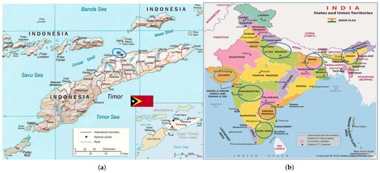
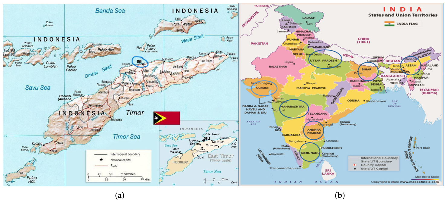
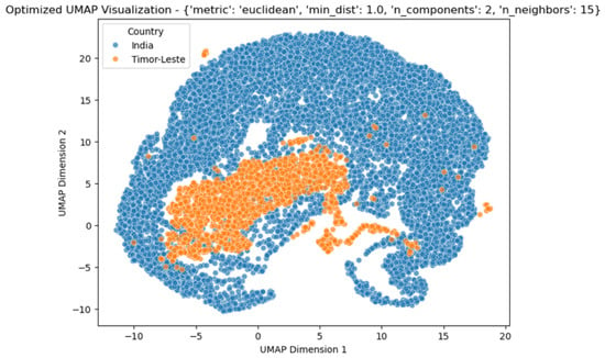
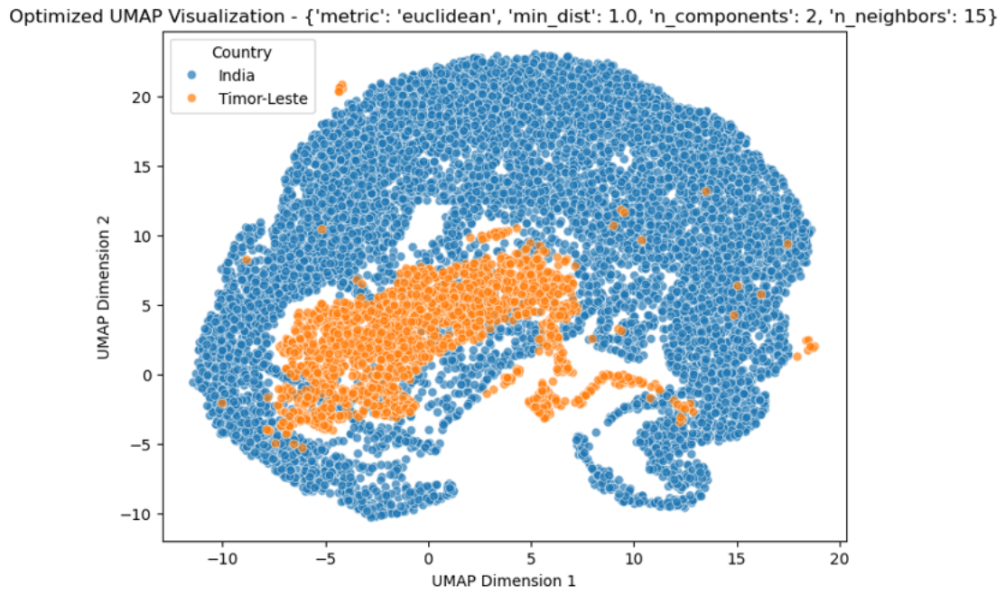
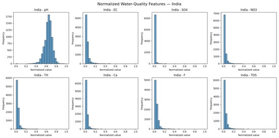
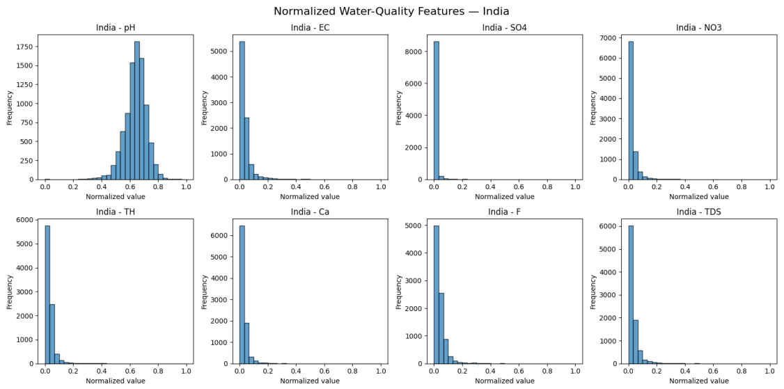
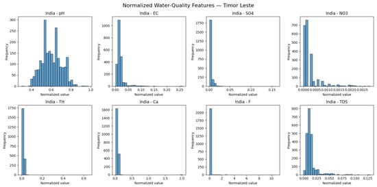
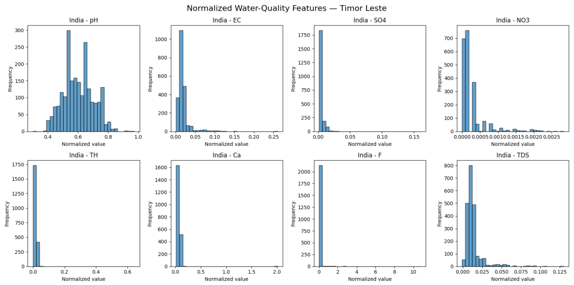
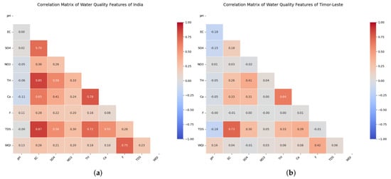
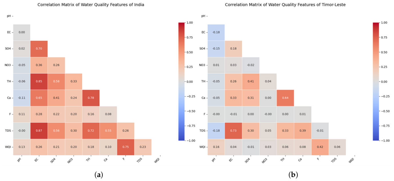
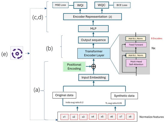
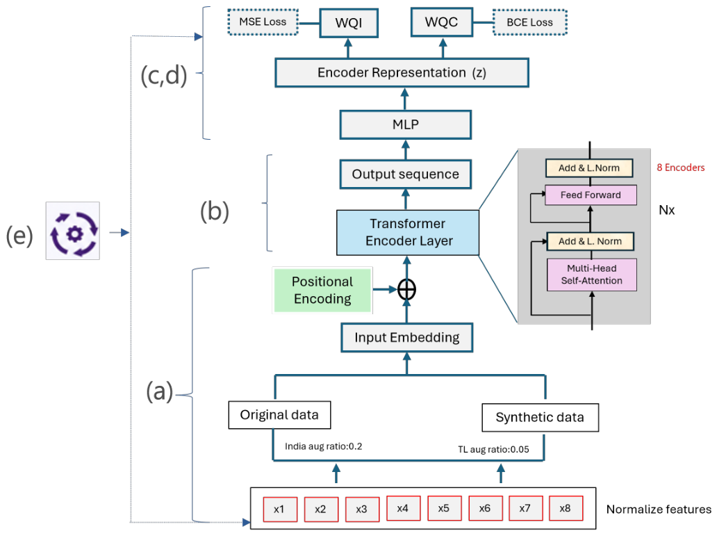
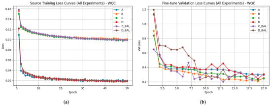
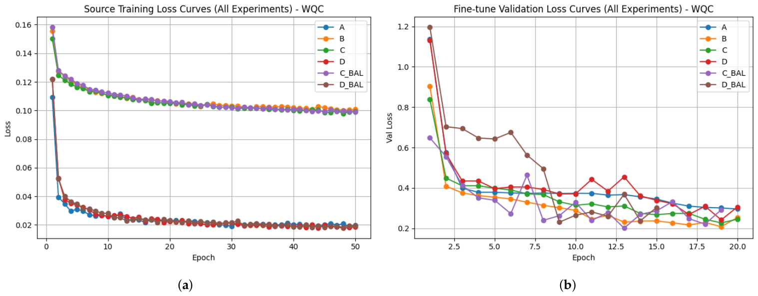
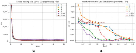
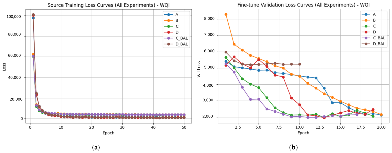
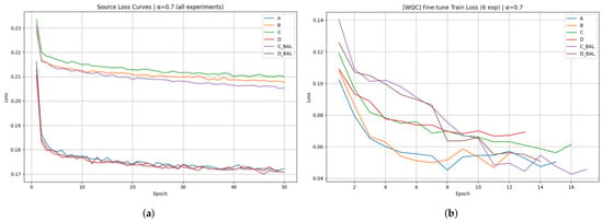
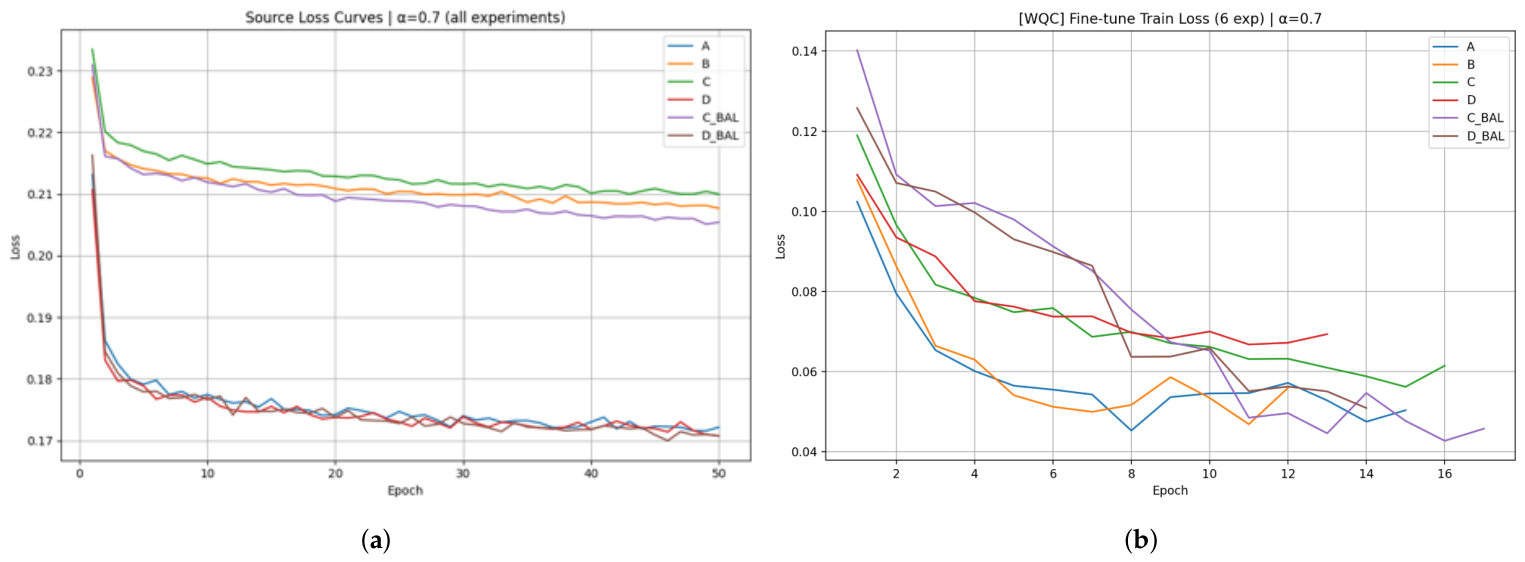
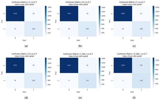
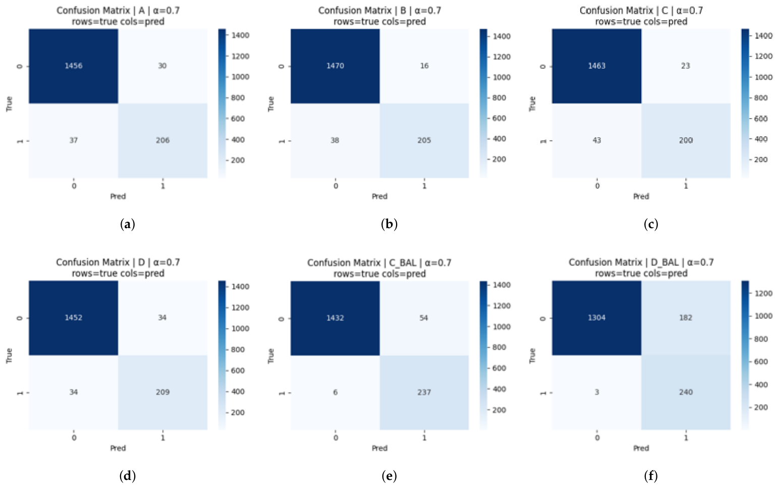
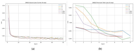
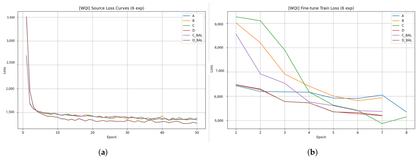
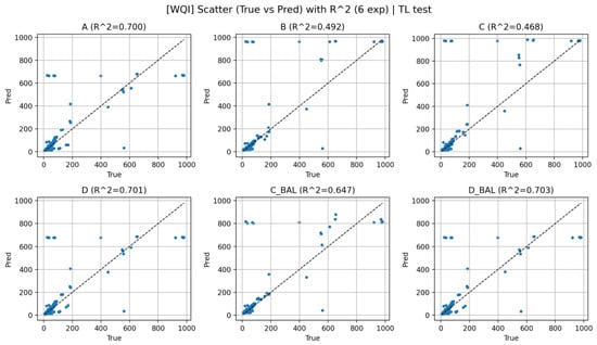
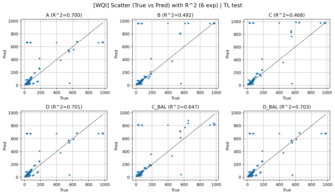
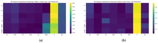
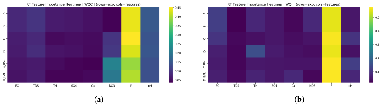

Disclaimer/Publisher’s Note: The statements, opinions and data contained in all publications are solely those of the individual author(s) and contributor(s) and not of MDPI and/or the editor(s). MDPI and/or the editor(s) disclaim responsibility for any injury to people or property resulting from any ideas, methods, instructions or products referred to in the content. |
© 2026 by the authors. Licensee MDPI, Basel, Switzerland. This article is an open access article distributed under the terms and conditions of the Creative Commons Attribution (CC BY) license.