


Abstract
Environmental monitoring in hazardous indoor zones conventionally relies on fixed-sensor networks or manual inspections, both of which suffer from spatial blind spots and increased human exposure risks. This paper addresses the problem of transforming sparse, mobile sensor measurements into spatially resolved risk assessments in GPS-denied environments. We propose a Hazard Index (HI) framework that normalizes environmental parameters against established safety thresholds into a unified, graduated risk metric with computational complexity, where N is the number of monitored parameters. The framework is designed for multi-parameter hazard assessment; the present work validates the computational pipeline, spatial mapping methodology, and classification logic through single-parameter CO2 detection () deployed on a LiDAR-guided robotic platform integrating an MQ-135 gas sensor interfaced via a NodeMCU ESP8266 microcontroller. Experimental validation across a 144 sq ft indoor area achieved a trajectory-following RMSE of 0.54 ft relative to planned waypoints using Hector SLAM without odometry, detected CO2 concentrations ranging from 0.02% to 0.25%, and identified a hazardous region encompassing eight measurement points () using a three-tier classification scheme (Safe, Elevated, Hazardous) within 225 s of active mapping. The framework provides a lightweight computational footprint suitable for real-time evaluation on an NVIDIA Jetson Nano. The proposed approach establishes a cost-effective, reproducible methodology for autonomous indoor environmental monitoring, with the modular architecture designed for future expansion to multi-parameter sensing.
1. Introduction
Environmental monitoring in hazardous zones represents a critical challenge at the intersection of industrial safety, public health, and autonomous systems. The detection and spatial mapping of hazardous gas concentrations in indoor and confined spaces have become increasingly urgent due to the growing frequency of industrial accidents attributed to inadequate monitoring systems. India has witnessed several devastating industrial disasters due to inadequate gas leakage monitoring, including the 1984 Bhopal gas tragedy resulting in over 3700 immediate fatalities [1], the 2020 Visakhapatnam styrene leak causing 12 deaths [2], and recurring incidents at waste management facilities such as Mumbai’s Deonar dumping ground [3] and Delhi’s Ghazipur landfill [4]. These incidents underscore a fundamental question: how can we transform sparse mobile sensor measurements into spatially resolved risk assessments that reliably detect localized hazards in GPS-denied environments?
The challenge lies not merely in gas detection, but in the spatiotemporal complexity of gas distribution. As illustrated in Figure 1, traditional fixed-sensor networks suffer from inherent spatial discontinuities that create dangerous blind spots between sensor nodes [5,6]. Gas plumes develop complex three-dimensional structures influenced by air currents, structural obstacles, and thermal gradients that point-source sensors cannot adequately characterize [7,8]. Manual inspection methods require inspectors to enter hazardous environments, accepting occupational exposure risks [9,10], while discrete inspection intervals create temporal gaps during which hazardous conditions may emerge undetected [6]. Human factors including fatigue and attention limitations introduce variability in assessment quality [5].
Figure 1.
Spatial sampling density comparison. Fixed-sensor networks (left) create discrete sensing zones with coverage gaps and occluded regions where gas accumulations remain undetected. Mobile robotic platforms (right) achieve comprehensive coverage through systematic area traversal, eliminating blind spots through dense, adaptive sampling. The fundamental advantage lies in transforming discontinuous point measurements into continuous spatial fields.
Mobile robotics offers a solution to these spatial limitations by enabling continuous coverage [5]. However, the deployment of autonomous systems in GPS-denied indoor environments remains theoretically and practically constrained by three fundamental challenges:
Challenge 1: Leveraging Consumer Robotics for Industrial Sensing: Precise localization is fundamental for hazard mapping, yet industrial-grade autonomous mobile robots (AMRs) typically require expensive, custom-built navigation stacks [11]. While GPS is inaccessible indoors, developing proprietary Simultaneous Localization and Mapping (SLAM) algorithms for low-cost IoT edge devices introduces significant computational overhead. This raises a critical operational question: How can commercially available, LiDAR-guided consumer platforms be effectively retrofitted to achieve sub-foot spatial resolution for hazardous gas distribution mapping without modifying their core navigation firmware?
Challenge 2: Multi-Parameter Risk Quantification: Current robotic approaches largely focus on detecting individual gas species in isolation, without integrating contextual environmental factors such as temperature, humidity, and airflow that critically influence hazard levels [7,9]. Most existing systems rely on simple threshold-based alerts [12], lacking a unified risk assessment model. The theoretical question is: How can we formalize multi-parameter hazard assessment into a mathematically rigorous framework that quantifies risk across heterogeneous environmental conditions?
Challenge 3: Spatial Reconstruction from Sparse Mobile Measurements: Mobile platforms generate sparse measurements at discrete waypoints, whereas hazard assessment requires continuous spatial fields. Reconstructing such fields introduces uncertainty that propagates into risk classifications, particularly when sampling density is limited. This raises a practical question: how reliably can interpolated hazard maps represent the underlying concentration distribution from sparse mobile measurements using computationally efficient methods suitable for real-time deployment on resource-constrained platforms?
To address these challenges, this paper proposes an autonomous spatiotemporal environmental monitoring framework that makes the following contributions:
- Integrated LiDAR-Guided Mapping Framework with Geometric Detection Bound: We present a modular system architecture integrating a custom MQ-135 sensing node with an Ackermann-steered mobile platform equipped with RPLIDAR A1M8, and demonstrate that scan-matching SLAM (Hector SLAM) achieves spatially correlated hazard mapping (RMSE < 0.55 ft) without wheel odometry. We further derive a geometric bound (Proposition 1, Section 3.4) establishing that for a ft grid spacing, the minimum reliably detectable hazard zone area is sq ft, providing a principled design rule linking grid spacing to detection capability.
- Multi-Parameter Hazard Index Model: We propose a generalized Hazard Index (HI) framework that synthesizes gas concentration, temperature, humidity, and airflow into a unified risk metric. The framework’s computational efficiency and classification logic are validated using single-parameter CO2 detection, demonstrating architectural readiness for multi-sensor expansion. This approach enables graduated risk classification (safe, elevated, hazardous) beyond conventional binary threshold-based detection.
- Scalable Architecture Validation: We demonstrate that consumer-grade robotic platforms can be adapted for professional environmental monitoring, proving the algorithm’s computational efficiency on resource-constrained hardware.
- Experimental Validation and Method Selection: Through CO2 concentration mapping across 144 square feet with a 2.88 sq ft measurement density, we validate the framework’s ability to: (i) complete comprehensive domain coverage in 225 s (±16s), (ii) detect concentration gradients from 0.02% to a source peak of 0.25%, (iii) identify hazardous zones (HI ≥ 1.0) that would remain undetected by sparse fixed-sensor networks, and (iv) achieve reliable wireless data transmission with minimal packet loss. A leave-one-out cross-validation against nearest-neighbour and Gaussian process regression baselines further demonstrates the effectiveness of the proposed method. IDW achieves near-zero bias (+15.1 ppm) at orders of magnitude lower runtime than GPR (0.02 ms vs. ∼350 ms per evaluation), justifying its selection for real-time deployment on resource-constrained hardware.
Figure 2 illustrates the proposed framework’s architecture. The system employs a custom Ackermann-steered platform equipped with RPLIDAR A1M8 for scan-matching localization via Hector SLAM, coupled with an MQ-135 multi-gas sensor for CO2 detection. Environmental data are processed through the Hazard Index model to generate spatially-resolved risk assessments, transforming raw sensor readings into actionable intelligence for facility managers and safety personnel.
Figure 2.
Conceptual framework of the LiDAR-guided environmental monitoring system. The autonomous platform integrates internal LiDAR-based spatial mapping with multi-parameter environmental sensing to generate georeferenced hazard assessments.
The current implementation validates this integrated approach through CO2 concentration mapping, demonstrating proof-of-concept feasibility under controlled indoor conditions. The modular architecture supports straightforward expansion to additional gas species (CH4, H2S, CO, VOCs) and full multi-parameter environmental sensing for comprehensive hazard assessment.
The use of a custom-configured platform built from commercial off-the-shelf components (COTS hardware: RPLIDAR A1M8, Jetson Nano, MQ-135) demonstrates that sophisticated, safety-critical monitoring can be achieved without requiring specialized, high-cost robotic platforms or high-performance computing hardware.
The remainder of this paper is structured as follows. Section 2 reviews related work in mobile robotics, gas sensing technologies, and environmental monitoring systems. Section 3 presents the system architecture, hardware configuration, and Hazard Index formulation. Section 4 discusses experimental validation, including spatial mapping, navigation accuracy, and comparative analysis. Section 5 examines operational implications and deployment considerations. Section 6 summarizes key contributions and identifies future research directions.
2. Related Work and Technical Gaps
The development of autonomous environmental monitoring systems requires integration across three research domains: autonomous robotic navigation, gas sensing technologies, and spatial risk assessment. This section reviews the state-of-the-art in each domain and identifies critical gaps that motivate our integrated framework.
2.1. Localization Strategies for Indoor Navigation
Precise localization is a fundamental capability for autonomous robots operating in GPS-denied environments. While SLAM approaches such as GMapping [13], Hector SLAM [14], and Cartographer [15] have achieved centimeter-level accuracy in structured environments, they often impose significant computational overheads unsuitable for lightweight IoT edge devices. More recent approaches incorporating particle filters and graph optimization have improved loop closure detection [11], yet the deployment of these complex algorithms on low-cost, resource-constrained hardware remains a practical challenge. Beyond LiDAR-based methods, feature-based visual SLAM approaches such as ORB-SLAM2 and ORB-SLAM3 have demonstrated strong performance on embedded platforms, providing rich feature-based mapping and loop closure capabilities using monocular, stereo, or RGB-D inputs. However, their performance depends on sufficient illumination and scene texture, which may be limited in industrial confined or hazardous environments. In such conditions, LiDAR-based scan-matching methods provide more consistent localization performance independent of lighting variability.
The Semantic Mapping Gap: Contemporary LiDAR-based algorithms have achieved high proficiency in generating accurate geometric occupancy grids. However, a critical limitation in current autonomous safety protocols is the decoupling of geometric mapping from dynamic environmental assessment. Standard navigation frameworks treat the environment as binary (occupied vs. free space) and lack standardized layers for embedding dynamic, non-geometric hazard variables. While recent research into semantic mapping attempts to label objects (e.g., distinguishing doors from tables), there remains a significant gap regarding real-time hazard semantics, specifically, the ability to augment static geometric maps with dynamic, multi-parameter risk gradients that enable instantaneous safety decisions during exploration [11]. Our work addresses this by coupling commercial LiDAR-guided navigation with environmental risk assessment, transforming geometric maps into actionable hazard intelligence. More recent surveys indicate that scan-matching and graph-based SLAM continue to be widely adopted paradigms for indoor mobile robotics, while highlighting the trade-off between localization accuracy and computational cost on resource-constrained embedded platforms [5].
2.2. Gas Sensing Technologies and Risk Assessment
Gas detection technologies have evolved from single-point electrochemical sensors to distributed sensor networks and mobile robotic platforms [7]. Metal oxide semiconductor (MOS) sensors, including the commercially ubiquitous MQ series, offer cost-effective detection across multiple gas species [16]. However, these sensors are characteristically limited by high cross-sensitivity to interfering gases and baseline drift over time [16]. Non-dispersive infrared (NDIR) sensors provide higher specificity for CO2 detection with improved long-term stability [17]. Recent work on electronic nose systems demonstrates multi-gas discrimination through sensor arrays and machine learning [18,19]. Recent studies have also explored data-driven approaches to address the spatial sparsity of mobile measurements. Winkler et al. [20] proposed a deep learning-based super-resolution framework that reconstructs high-resolution gas distribution maps from sparse robotic samples, demonstrating the potential of learned priors to complement geometric interpolation methods. Ojeda et al. [21] introduced a probabilistic gas distribution mapping technique that explicitly models measurement uncertainty and sensor noise, addressing a key limitation of deterministic approaches.
The Multi-Parameter Integration Gap: While the development of sophisticated metal-oxide (MOX) sensors has enabled mobile gas detection, a significant theoretical challenge remains in the effective, real-time integration of heterogeneous environmental data. Current literature on Gas Distribution Mapping (GDM) is predominantly focused on probabilistic estimation techniques to generate 2D concentration maps (ppm) [7,8]. While some studies address environmental factors like humidity and temperature, they typically treat these variables solely as calibration parameters to correct sensor drift [17], rather than as distinct, contributing factors to an overall environmental hazard state. There is a notable scarcity of frameworks that mathematically integrate these environmental gradients into a unified risk model during active robotic exploration. Most existing approaches rely on simple threshold-based alerts [12,22], lacking comprehensive risk quantification that accounts for contextual factors collectively determining hazard levels [9].
Beyond gas sensing specifically, the broader robotics literature on multimodal sensing and sequential perception provides useful context for integrating heterogeneous sensor modalities within unified decision-making frameworks. Prior work in this area highlights the benefits of combining complementary sensing channels and leveraging temporal structure to improve robustness and interpretability.
While such approaches are not directly applied in the present work, they suggest promising directions for extending the proposed framework toward multi-parameter fusion and temporally aware hazard assessment.
2.3. Mobile Robotic Environmental Monitoring Systems
Several research efforts have explored mobile robots for environmental monitoring. Lilienthal et al. [7,23] pioneered gas distribution mapping using mobile robots, demonstrating the feasibility of spatial concentration profiling. Subsequent work by Reggente and Lilienthal [8] improved mapping accuracy through predictive models of gas dispersion incorporating wind information. More recent implementations incorporate UAVs for atmospheric monitoring [24,25] and ground robots for confined space assessment [9,10,22]. Recent work has extended mobile gas sensing to more challenging operational scenarios. Nordström et al. [10] demonstrated autonomous UAV-based safety inspections and gas monitoring in hazardous mining environments, validating robotic environmental assessment under conditions unsafe for human entry. Góngora et al. [26] proposed an information-driven exploration strategy in which sampling locations are selected to maximize information gain, reducing coverage time compared to fixed traversal patterns. Francis et al. [5] provide a comprehensive recent survey of gas source localization and mapping, identifying adaptive sampling and uncertainty-aware mapping as key emerging research directions.
Table 1 summarizes key mobile monitoring systems. These systems exhibit common limitations: reliance on odometry-based localization with accumulated drift or GPS unsuitable for indoor environments [23,24], single-parameter monitoring without contextual environmental factors [7,25], threshold-based detection without comprehensive risk models [12,22], and use of custom robotic platforms limiting practical deployment [9,24].
Table 1.
Comparison of mobile gas monitoring approaches.
2.4. Spatial Interpolation for Environmental Fields
Environmental monitoring requires transforming sparse mobile measurements into continuous spatial fields. Inverse Distance Weighting (IDW) [27] provides computational efficiency but assumes smooth spatial variation. Kriging methods offer uncertainty quantification but require spatial correlation models [28]. Prior mobile gas mapping work [23,29] applies interpolation without quantifying detection confidence or deriving minimum sampling density requirements. Recent probabilistic frameworks [21] and learning-based reconstruction methods [20] have begun to address these limitations by incorporating uncertainty modeling and data-driven spatial priors. However, such approaches typically involve increased computational complexity, which may limit their applicability for real-time deployment on resource-constrained embedded platforms.
The Theoretical Gap: Existing work lacks formal analysis linking measurement density, interpolation method, and hazard detection reliability. No prior research derives error bounds on interpolated risk estimates as a function of sensor characteristics and spatial sampling. This theoretical gap prevents principled determination of coverage requirements for safety-critical applications.
2.5. Summary: The Framework Integration Gap
The existing body of work demonstrates robust individual solutions for navigation and gas concentration estimation. However, the literature reveals a fundamental disconnect when merging these domains for safety applications: no established theoretical framework unifies real-time localization data, multi-sensor environmental fusion, and a formal spatial risk model into a single deployable system validated on resource-constrained hardware.
The novelty of the proposed framework does not reside in the individual algorithmic components—Hector SLAM and IDW interpolation are established methods deliberately selected for computational tractability on embedded hardware—but in the integrated realization of three core contributions not simultaneously addressed in prior mobile gas mapping literature. First, a spatiotemporal Hazard Index is formulated as a continuous spatial risk field evaluated at each robot pose during active exploration, structurally distinct from the EPA’s static population-level Hazard Index [30], which produces a single scalar per exposure scenario. Second, a geometric minimum-zone detection bound (Proposition 1, Section 3.4) provides a principled sampling density criterion for safety-critical mobile gas mapping, derived from grid geometry. Third, a sensor-noise-aware uncertainty propagation framework (Section Uncertainty Propagation and Classification Confidence) enables probabilistic characterization of classification confidence under realistic sensor imprecision. Together, these contributions establish a framework with quantifiable detection guarantees (Proposition 1), explicit treatment of sensor-induced classification uncertainty (Section Uncertainty Propagation and Classification Confidence), and a spatial risk representation that differs in formulation from prior population-level indices [30].
The aim of this work is therefore not to propose a new SLAM or interpolation algorithm, but to establish a theoretically grounded and experimentally validated framework for real-time hazard mapping with quantifiable detection guarantees on resource-constrained hardware. The present study addresses this integration gap through an experimentally validated system-level framework (Section 4).
3. Materials and Methods
This section presents the theoretical framework, system architecture, and experimental protocol for autonomous spatiotemporal hazard mapping. We first formulate the Multi-Parameter Hazard Index model that transforms heterogeneous sensor data into unified risk assessments (Section 3.1). We then describe the hardware configuration and SLAM-based localization pipeline (Section 3.2), experimental protocol and coverage strategy (Section 3.3), and spatial interpolation methodology with validation metrics (Section 3.4).
3.1. Multi-Parameter Hazard Index Framework
Existing gas distribution mapping approaches generate concentration fields without standardized risk quantification tied to a conservative threshold [23,29]. Most systems employ binary threshold-based alerts [12,22] that trigger only when a single parameter exceeds a fixed limit, failing to account for the combined influence of multiple environmental stressors on overall hazard severity. To address this gap, we propose a Multi-Parameter Hazard Index (HI) that models environmental risk as a continuous scalar function of multiple sensor inputs with explicit regulatory normalization.
For a spatial location at time t, the Hazard Index is defined as
where N is the number of monitored hazard parameters, is the measured value of parameter i (e.g., gas concentration, temperature, humidity, airflow velocity) at the robot’s current pose, is the maximum permissible safety threshold for parameter i derived from regulatory standards such as OSHA Permissible Exposure Limits [31,32] or ASHRAE ventilation guidelines, is a normalized weight coefficient () representing the relative criticality of each parameter, and is an environmental correction factor accounting for synergistic effects among ambient conditions.
Temperature risk is bidirectional; a single-ratio normalization is therefore insufficient. The piecewise temperature hazard function is defined as
within the safe temperature band , the function contributes zero to HI. Deviations below or above produce a positive contribution proportional to the magnitude of exceedance, capturing the physical effect that extreme temperatures increase gas volatility and impair human physiology. The airflow term in Equation (1) is similarly non-trivial: low airflow increases HI, reflecting the physical reality that stagnant air promotes localized gas accumulation.
The formulation in Equation (1) possesses several properties relevant to safety-critical deployment. The ratio normalizes each parameter to a common dimensionless scale, ensuring that HI = 1.0 corresponds to the adopted safety threshold used for hazard classification regardless of the physical units of individual sensors. The linear summation structure yields computational complexity per spatial evaluation, where N is the number of monitored parameters; for the intended four-parameter configuration this corresponds to a constant-time operation per grid point, enabling real-time evaluation on embedded hardware such as the Jetson Nano. The index is monotonically increasing with respect to each parameter: any increase in produces a proportional increase in HI, ensuring that deteriorating conditions are reflected in elevated risk scores. Furthermore, incorporating a new sensor requires only specifying the corresponding , , and without modification to the computational architecture.
The proposed formulation shares structural similarity with the U.S. Environmental Protection Agency’s Hazard Index for chemical mixtures [30], defined as the sum of Hazard Quotients (exposure divided by reference dose) across multiple substances. However, the EPA framework is designed for population-level chronic exposure assessment using time-weighted average concentrations, and produces a single scalar per exposure scenario. In contrast, the framework proposed here operates at spatiotemporal resolution: is computed at each robot pose during active exploration, producing a continuous spatial risk field rather than a population summary statistic. Additionally, the inclusion of the environmental correction factor and non-chemical parameters (temperature, humidity, airflow) extends the formulation beyond chemical-only risk aggregation. While individual parameters are normalized with respect to established safety thresholds, the composite Hazard Index itself is not a standardized regulatory metric but a unified, application-specific indicator for spatial risk interpretation.
The weight vector enables context-dependent prioritization across different industrial scenarios. In petrochemical environments, flammable gas concentration may warrant higher weight, whereas in confined-space entry scenarios, oxygen displacement and toxic gas exposure may take precedence. For the intended four-parameter configuration (: gas concentration, temperature, humidity, airflow), domain-specific weight assignment can be informed by regulatory risk hierarchies or historical incident data.
The correction factor models how ambient conditions modulate hazard severity; for instance, elevated temperature increases gas volatility, while low airflow promotes localized accumulation. Under the controlled laboratory conditions of this study (stable temperature and humidity), reduces to unity. Empirical characterization of for the multi-parameter configuration is discussed in Section 5.4.
Spatial locations are classified into discrete risk categories based on the computed HI:
The primary threshold at demarcates the indoor hazard boundary, where measured conditions equal or exceed the adopted 2000 ppm indoor screening limit [31]. The elevated threshold at HI = 0.7 is derived from established occupational safety practice: OSHA mandates that employers initiate monitoring and exposure control measures when airborne concentrations reach 50% of the Permissible Exposure Limit (the Action Level), while the 0.7 threshold provides an intermediate warning tier between this action level and the compliance boundary. This three-tier scheme enables graduated response protocols: safe zones require routine monitoring only, elevated zones warrant increased surveillance and proactive mitigation, and hazardous zones demand immediate corrective action.
Worked Example: Table 2 illustrates the HI computation for a hypothetical waypoint with the following measurements and illustrative weights: , , , and .
Table 2.
Hypothetical multi-parameter HI computation.
This example illustrates that even when no single parameter greatly exceeds its threshold, the combined multi-parameter assessment produces an Elevated classification. Had the gas concentration been 75 ppm instead of 60 ppm, HI would rise to 1.194, classifying the location as Hazardous.
Although the composite HI map is the primary output, the framework is designed to log individual parameter maps alongside the composite index. In the current validation, the individual CO2 concentration map demonstrates this capability. For the full configuration, equivalent maps for temperature, humidity, and airflow would be generated independently at each waypoint, enabling post hoc diagnosis of which parameter drove an elevated HI classification before corrective action is taken.
For the experimental validation presented in Section 4, the framework is instantiated for (CO2 detection only) to isolate and verify the core mapping pipeline, SLAM localization accuracy, and computational performance independently of multi-sensor fusion complexity:
where is the measured CO2 concentration and (2000 ppm) is adopted as the hazard threshold consistent with confined-space pre-entry assessment practice. The correct OSHA 8-h time-weighted average Permissible Exposure Limit (PEL) for CO2 is 5000 ppm [32]; the 2000 ppm threshold employed here is deliberately more conservative and is justified on two grounds. First, the OSHA Technical Manual for Indoor Air Quality Investigations specifies 0–2000 ppm as the standard indoor CO2 screening range for workplace assessments, making 2000 ppm the upper boundary of OSHA’s own indoor air quality screening band [31]. Second, peer-reviewed evidence identifies the 1500–2500 ppm range as the interval at which measurable cognitive performance decrements and physiological symptoms such as headaches and drowsiness arise, which occur consistently in enclosed-space occupants [33]. The adopted threshold therefore represents a conservative precautionary screening level appropriate for confined-space pre-entry assessment, where thresholds below the chronic occupational PEL are standard practice to account for poor ventilation, elevated physical activity, and the absence of continuous atmospheric monitoring during occupancy.
To consolidate the mathematical formulation into an executable procedure, Algorithm 1 presents the complete SLAM-based hazard mapping pipeline. The algorithm integrates the Hazard Index formulation (Equation (1)), the piecewise temperature model (Equation (2)), and airflow inversion with SLAM-based localization, per-parameter spatial interpolation, and three-tier classification.
This representation highlights that the proposed framework is a structured, modular pipeline, in which data acquisition, spatial referencing, parameter-wise interpolation, and risk evaluation are treated as distinct computational stages.
| Algorithm 1 SLAM-based hazard mapping framework |
| Require: LiDAR scans , sensor vector , waypoints W, thresholds , weights , correction |
| Ensure: Per-parameter maps , hazard map , classification map |
|
The algorithm proceeds in three stages. In the acquisition stage (lines 2–6), the robot traverses predefined waypoints, estimates its pose using Hector SLAM, and stores averaged multi-parameter measurements together with spatial coordinates. Averaging over k samples reduces transient sensor noise.
In the interpolation stage (lines 8–10), each parameter is interpolated independently using IDW to generate continuous spatial fields . This per-parameter formulation preserves traceability, allowing identification of the specific variable responsible for elevated risk levels.
In the evaluation stage (lines 12–21), the Hazard Index is computed at each grid point using parameter-specific transformations: standard normalization for concentration-like variables, the piecewise temperature response (Equation (2)), and airflow inversion. The aggregated score is scaled by the environmental correction factor and mapped to the three-tier classification scheme defined in Equation (3).
The modular structure supports extensibility, as additional sensors can be incorporated by augmenting the measurement vector and defining corresponding thresholds and transformations, without altering the overall pipeline.
Uncertainty Propagation and Classification Confidence
Building upon the Hazard Index defined in Equation (1), the deterministic formulation is extended here to account for sensor imprecision; practical deployment requires quantification of how measurement uncertainty propagates into HI values and affects zone classification. Two structurally distinct uncertainty sources are present in the MQ-135 implementation and must be treated separately.
- Precision uncertainty:
Measurement-to-measurement variability at a fixed location is characterized by the coefficient of variation , measured empirically as 7.5% across five replicate measurements at the origin (Section 4.4). This gives at any measurement point with concentration G. Applying standard first-order error propagation [34] to the instantiation ,
For the general N-parameter formulation, assuming mutually independent sensor noise across parameters, which is reasonable given the use of physically distinct sensing modalities,
- Systematic calibration bias:
MQ-135 sensors exhibit unit-to-unit variability of ±15–20% [16], characterized here as (midpoint estimate). Unlike precision uncertainty, systematic bias scales all measurements by a spatially invariant factor . Because is linear in G, the entire HI field is scaled uniformly: . Critically, the relative spatial structure of the hazard field—the gradient direction, the location of peak concentration, and the rank ordering of waypoints by risk—is preserved under any spatially uniform scale factor. Spatial hazard zone boundaries are therefore expected to remain approximately stable under systematic offset, which justifies the use of MQ-135 measurements for hazard zone delineation despite the absence of independent NDIR cross-calibration in the present proof-of-concept study.
- Classification confidence:
The 95% confidence interval on any HI value under precision uncertainty alone is
A waypoint is defined as robustly classified (with respect to precision uncertainty) if its entire 95% CI lies within a single tier of Equation (3), and marginally classified otherwise. Applying Equation (7), the tier-boundary conditions are
- Robustly Hazardous (): Lower CI bound .
- Robustly Safe (): Upper CI bound .
- All other waypoints are marginally classified and may cross a tier boundary under an unfavourable sensor reading.
Classification confidence results for the experimental dataset are summarized in the results section (Section 4.1).
3.2. System Architecture and Hardware Configuration
The system integrates an autonomous navigation platform with a wireless environmental sensing module, operating within the ROS Noetic middleware framework. Figure 3 presents the assembled robotic platform with labeled hardware components alongside the data processing pipeline.
Figure 3.
(Left) Custom Ackermann-steered robotic platform with labeled components. (Right) Data processing pipeline from sensor acquisition through SLAM localization, sensor-pose fusion, spatial interpolation, and Hazard Index computation to three-tier risk classification.
As shown in Figure 3, the platform carries both navigation and sensing hardware in a compact configuration (350 × 280 × 120 mm, 230 mm wheelbase). The RPLIDAR A1M8 is elevated above the chassis to maintain an unobstructed 360-degree scan field, while the MQ-135 sensing module is positioned at chassis height (150 mm) to sample the zone relevant to ground-level gas accumulation. The processing pipeline operates sequentially: sensor data acquisition feeds into Hector SLAM for scan-matching localization, which provides georeferenced pose estimates fused with gas concentration readings at each waypoint. The fused measurement tuples are spatially interpolated using Inverse Distance Weighting and transformed into Hazard Index values through Equation (4), culminating in the three-tier classification defined by Equation (3).
The navigation platform is a custom Ackermann-steered four-wheeled robot controlled by an NVIDIA Jetson Nano (4 GB RAM, quad-core ARM Cortex-A57) executing ROS Noetic. An L298N H-bridge motor driver provides PWM control (1 kHz) for independent left/right propulsion. Power is supplied by an 11.1 V 3S LiPo battery (2200 mAh) through a 5 V/4 A LM2596 buck converter, providing approximately 90 min of autonomous operation.
An RPLIDAR A1M8 (5.5 Hz scan rate, 360°
coverage, 0.15–12 m range, 1° angular resolution) provides laser scan data via USB 2.0. Hector SLAM was selected for several reasons specific to this platform. The Ackermann steering geometry introduces coupled kinematic constraints and wheel slip on smooth indoor surfaces that degrade odometry accuracy [11]; Hector SLAM eliminates this dependence by relying exclusively on scan matching. Its multi-resolution occupancy-grid formulation enables efficient convergence on resource-constrained hardware without particle filters or graph optimization, supporting real-time execution on the Jetson Nano, while its centimetre-level accuracy in structured environments [14] satisfies the sub-foot requirement at the planned 2 ft grid resolution. The 2D LiDAR-only sensing configuration also precludes feature-based visual SLAM methods such as ORB-SLAM2/3, which would require a calibrated visual sensor and depend on adequate scene illumination and texture that conditions not guaranteed in target deployment environments with low light, dust, or limited visual texture.
At each time step t, Hector SLAM estimates the robot pose by minimizing the alignment error between laser scan endpoints and the occupancy map M:
The optimization employs Gauss-Newton iteration with a convergence threshold of 0.001 m/rad over multi-resolution occupancy grids (coarse: 0.20 m, medium: 0.10 m, fine: 0.05 m per cell). The multi-resolution hierarchy enables efficient scan matching while maintaining fine-grained spatial detail; pose estimates reported in Section 4 are derived from the finest 0.05 m resolution grid. The ROS tf framework maintains coordinate transforms between /map (global fixed frame), /odom, /base_link (robot center), and /laser (LiDAR center) frames, with Hector SLAM publishing corrected /map→/odom transforms at 5.5 Hz.
For environmental sensing, an MQ-135 tin dioxide (SnO2) semiconductor gas sensor (10–10,000 ppm CO2 range, <60 s response time to 90% step change) is interfaced to a NodeMCU ESP8266 microcontroller with integrated Wi-Fi (IEEE 802.11 b/g/n). The NodeMCU serves as a wireless analog-to-digital bridge, necessary because the Jetson Nano lacks native analog input pins required for the MQ-135 resistive output. The sensor resistance relates to output the voltage via:
where V and kΩ. The NodeMCU samples voltage at 1 Hz through its 10-bit ADC, applies a 10-sample moving average filter, and converts readings to CO2 concentration using the manufacturer calibration: , where is the sensor resistance in clean air. Timestamped data are transmitted to the Jetson Nano via HTTP POST over a localized Wi-Fi connection (Flask server, port 5000). A separate 9 V battery powers the sensing module for electrical isolation from the navigation platform. The MQ-135 sensor requires a 5-min warm-up period prior to data acquisition and operates within −10 to 50 °C and 15–90% relative humidity (RH).
The MQ-135 is a low-cost metal-oxide (MOX) gas sensor that provides indicative concentration estimates based on resistance variation. Such sensors are known to exhibit cross-sensitivity to multiple gases and unit-to-unit variability, and their output depends on calibration conditions. In the present implementation, CO2 concentration values are derived using the manufacturer-provided calibration curve without independent cross-validation against a reference-grade instrument. Accordingly, the reported values should be interpreted as indicative measurements suitable for spatial trend analysis rather than precise quantitative concentrations.
ROS-Based System Integration
The system is implemented within the ROS Noetic middleware, which provides the communication layer, coordinate-frame management, and message synchronization infrastructure for the overall pipeline. The architecture follows a modular publish–subscribe paradigm, enabling real-time data exchange between the sensing, localization, navigation, and hazard mapping components.
The ROS graph comprises five principal nodes executing on the Jetson Nano: an RPLIDAR driver publishing laser scans, a Hector SLAM node producing pose estimates and the occupancy grid, a waypoint navigation node issuing velocity commands, a motor control node translating these commands into actuator signals, and a custom gas_mapping_node performing sensor–pose fusion. Table 3 summarizes the node-level interactions.
Table 3.
ROS node interactions in the proposed system.
Coordinate consistency across nodes is maintained through the ROS tf framework, which manages transforms between the global /map frame, the robot /base_link, and the /laser sensor frame. Gas sensor readings (1 Hz) and SLAM pose estimates (5.5 Hz) are associated using approximate time synchronization with a tolerance of s. At each waypoint, the robot halts for 3 s, during which multiple sensor readings are acquired and averaged to reduce measurement noise. This synchronized sensor–pose fusion produces a spatially consistent dataset that serves as input to subsequent interpolation and Hazard Index computation.
This node-based decomposition underpins the modularity of the framework. Additional sensors can be incorporated by introducing new publisher nodes and corresponding subscriptions within gas_mapping_node, without modifying the SLAM or mapping pipeline. Similarly, the waypoint-based exploration strategy can be replaced by adaptive or information-driven planning methods without affecting the remaining system components, supporting the sensor-agnostic and exploration-agnostic design described in Section 3.1.
Additionally, the platform is equipped with a TF Luna 1D LiDAR time-of-flight sensor interfaced to an Arduino Uno, mounted at the front of the chassis for forward-facing distance measurement. This module is physically integrated but was not activated during the current experimental validation; it is intended for reactive obstacle avoidance in future deployments targeting unstructured environments with dynamic obstacles.
3.3. Experimental Protocol and Coverage Strategy
Experiments were conducted in a controlled rectangular indoor laboratory measuring 18 ft × 8 ft (144 sq ft, 13.38 m2) at Veermata Jijabai Technological Institute, Mumbai. Environmental conditions were maintained at 24 ± 2 °C and 55 ± 10% relative humidity. A localized CO2 emission source (dry ice sublimation) was established at coordinates (10 ft, 8 ft) to generate peak concentrations of approximately 2500 ppm (0.25%). The room was isolated from mechanical ventilation to minimize uncontrolled advective transport. The coordinate system origin was established at (0, 0) in the southwest corner, with the x-axis oriented east (0–18 ft) and the y-axis oriented north (0–8 ft).
The robot executed a boustrophedon (zig-zag) coverage path, a systematic traversal strategy selected for two reasons: it guarantees complete area coverage without gaps, and the regular grid pattern produces uniformly spaced measurements amenable to spatial interpolation without requiring non-uniform sampling corrections. The trajectory consisted of row-major waypoints: traverse x from 0 to 18 ft at ft, increment y by 2 ft, reverse traverse x from 18 to 0 ft at ft, and repeat until ft. This strategy yielded 50 discrete measurement waypoints arranged in a 10 × 5 grid with 2 ft (0.61 m) spacing, corresponding to a measurement density of 2.88 sq ft per point. Proportional navigation (, s−1) limits velocity to 0.15 m/s linear and 0.5 rad/s angular. Total mission duration was 4.5 ± 0.3 min (270 ± 18 s), comprising 225 s of active traversal and measurement, with the remainder allocated to SLAM initialization (approximately 20 s) and post-mission data transmission (approximately 25 s).
The MQ-135 manufacturer specification indicates a response time of approximately 60 s to reach 90% of a full-scale step change, but this represents a worst-case scenario not encountered during systematic traversal. Adjacent waypoints are separated by 2 ft, where mean inter-waypoint concentration differences are approximately 150 ppm (about 6% of the observed dynamic range), resulting in smaller sensor responses and faster effective equilibration. The 3-s averaging window at each waypoint was empirically determined to yield a coefficient of variation below 8% across replicate measurements at fixed positions, indicating sufficient stabilization for the spatial gradients encountered. While this approach does not fully eliminate transient response artifacts, the systematic traversal pattern suggests that residual bias is likely to affect measurements in a broadly consistent manner, thereby preserving the relative spatial structure of the concentration field that determines hazard zone delineation. It should be noted, however, that this protocol represents a pragmatic compromise rather than a formal validation of sensor dynamics; residual transient artifacts attributable to sensor lag cannot be fully excluded, and this limitation is discussed further in Section 5.3.
3.4. Spatial Interpolation and Validation Metrics
It is important to note that the objective of this work is not to propose a new gas distribution model, but to demonstrate an integrated real-time hazard mapping framework on resource-constrained hardware; IDW is selected as a computationally appropriate interpolation method consistent with this objective.
The 50 discrete measurements must be transformed into a continuous spatial field for hazard zone delineation. We employ Inverse Distance Weighting (IDW), selected over geostatistical alternatives for three reasons: IDW requires no training data or variogram fitting, making it suitable for single-pass mapping missions where spatial correlation structure cannot be pre-estimated; it is computationally lightweight ( per query point), consistent with the resource-constrained deployment objective (a quantitative comparison against nearest-neighbour and Gaussian process regression baselines is presented in Section 4.6.1); and for monotonically varying concentration fields emanating from a localized source, IDW produces physically plausible interpolations without the risk of negative concentration estimates that unconstrained kriging may produce [27].
For an arbitrary query point , the estimated concentration is:
where is the Euclidean distance from the query point to measurement point i, and is the power parameter. The choice of balances local fidelity with regional smoothness and approximates the inverse-square attenuation characteristic of diffusive gas transport from a point source. When , direct assignment is applied. Interpolated fields are evaluated on a 0.1 ft × 0.1 ft grid (181 × 81 = 14,661 points) for visualization and hazard delineation.
IDW estimates near domain boundaries have fewer contributing neighbors and may exhibit reduced accuracy; however, the emission source and primary hazardous zones are located in the interior of the mapped area. While IDW is computationally appropriate for real-time implementation on resource-constrained platforms, it assumes smooth spatial variation and relies solely on geometric proximity, without modeling the underlying physical processes governing gas dispersion such as advection, turbulence, or airflow dynamics. The reconstructed concentration fields should therefore be interpreted as approximate spatial estimates rather than physically grounded gas distribution models. More advanced approaches including probabilistic gas distribution mapping, physics-informed models, and learning-based reconstruction methods can provide improved fidelity at increased computational cost, and are identified as directions for future work in Section 5.4.
Navigation accuracy is quantified by comparing planned waypoints to SLAM-recorded positions using Root Mean Square Error:
Component-wise RMSE along the x- and y-axes is computed to identify directional bias. Sensor repeatability is assessed via the coefficient of variation (CV ) from replicate measurements at the origin (0, 0). Communication reliability is evaluated via the packet delivery ratio (PDR ). All processing was implemented in Python 3.8 (NumPy 1.21.5, SciPy 1.7.3, Matplotlib 3.5.1, Pandas 1.3.5) with ROS Noetic on the Jetson Nano.
Minimum Detectable Hazard Zone Size
A formal relationship between measurement grid spacing and detection capability can be derived from geometric coverage principles. This provides a quantitative basis for the sampling density selected in Section 3.3, which has not been explicitly addressed in prior mobile gas mapping work [23,29].
Proposition 1
(Minimum Detectable Hazard Zone Area). For a boustrophedon measurement grid with uniform spacing , under the assumption of spatially continuous hazard regions, the minimum area of a circular hazard zone that is guaranteed (in a geometric sense) to contain at least one measurement waypoint is
Proof.
Consider a circular hazard zone of radius centred at an arbitrary location within the mapped domain. For a uniform rectangular grid with spacing , the maximum possible distance from any domain point to its nearest measurement waypoint is the half-diagonal of one grid cell:
For the hazard zone to contain at least one waypoint regardless of source position, the necessary and sufficient condition is , yielding the minimum detectable radius:
The minimum detectable area follows directly as . □
Remark: This guarantee is geometric in nature and assumes that the hazard region is spatially continuous and stationary over the measurement interval. It does not account for turbulent dispersion, transient plume dynamics, or sensor uncertainty at the measurement point; these aspects are addressed separately in Section Uncertainty Propagation and Classification Confidence.
Corollary 1.1
(Deployment Design Rule). To guarantee geometric coverage of a hazard zone of target area , the measurement grid spacing must satisfy
For the experimental configuration employed in this study ( ft, 0.61 m), Equation (12) yields sq ft (0.58 m2). A grid spacing of 2 ft was selected to ensure reliable geometric coverage of hazard zones larger than this minimum, directly informed by Corollary 1.1. The experimentally observed hazard zone of 18–20 sq ft exceeds by a factor of approximately 3, providing a sufficient detection margin under the controlled conditions of this study. Representative spacing requirements for other target zone sizes are summarized in Table 4.
Table 4.
Grid spacing required to guarantee geometric coverage of hazard zones of given target area (Corollary 1.1).
To our knowledge, prior mobile gas mapping work does not explicitly formulate grid spacing requirements in terms of geometric coverage guarantees for hazard detection; instead, measurement density is typically selected empirically or based on platform speed constraints [9,23,29].
4. Experimental Validation and Results
This section presents the experimental validation of the SLAM-based hazard mapping framework. The current experimental validation focuses on CO2 () to isolate the mapping pipeline, while multi-parameter integration is demonstrated analytically.
4.1. Spatial CO2 Mapping and Hazard Classification
The autonomous system mapped CO2 concentrations across the 144 sq ft experimental area using the boustrophedon coverage strategy described in Section 3.3. Table 5 summarizes the key mapping and classification outcomes.
Table 5.
CO2 concentration mapping and hazard classification results.
All concentration values reported in Table 5 and subsequent figures are derived from the manufacturer-provided MQ-135 calibration curve without independent verification against a reference CO2 instrument. MQ-135 sensors exhibit typical unit-to-unit variability of ±15–20% [16], and consequently, absolute concentration values carry corresponding uncertainty. As the objective of the present experiments is to evaluate the integrated SLAM–sensing–mapping pipeline rather than to obtain metrologically precise CO2 measurements, these values are used to reconstruct spatial gradients and identify indicative high-concentration regions, rather than to provide compliance-grade exposure assessment. While systematic calibration offsets may affect absolute values, they are expected to influence measurements in a broadly consistent manner, thereby preserving the relative spatial structure that governs hazard zone delineation.
Table 6 reveals that classification robustness is highest at the extremes of the HI distribution. The peak measurement ( at the source location) is the sole robustly hazardous waypoint, with a lower 95% CI bound of 1.066, confirming hazardous classification under any realization of precision noise. The seven remaining hazardous waypoints () are marginally classified; their lower CI bounds fall below 1.0, indicating that an unfavourable sensor reading could place them in the elevated tier. However, all eight waypoints maintain on the mean measurement, and their upper CI bounds confirm elevated risk even under the most conservative scenario. The 25 robustly safe waypoints (, upper CI ) provide high-confidence safe-zone delineation independent of measurement noise. This uncertainty-aware classification enables differentiated operational responses: robustly hazardous zones demand immediate corrective action, while marginally classified zones warrant repeated measurement before a compliance decision is made.
Table 6.
Hazard Index classification confidence under precision uncertainty (CV = 7.5%). The 95% CI is computed using Equation (7). Robustness thresholds: for robustly hazardous; for robustly safe.
Figure 4 presents the spatial CO2 distribution obtained through IDW interpolation (, Equation (10)) from 50 discrete measurements. The concentration field exhibits a pronounced gradient from 0.02% at the southwest corner to a peak of 0.25% at (10 ft, 8 ft), consistent with the positioned dry ice emission source. A distinct high-concentration ridge extends along the northern boundary ( ft) from to 14 ft, with concentration decreasing monotonically with distance from the peak. The near-source gradient of 0.015%/ft transitions to less than 0.003%/ft at the periphery, indicating localized accumulation rather than uniform dispersion. The measurement density of 2.88 sq ft per point enables detection of such localized accumulation zones that would be missed by typical fixed-sensor networks with 10–15 ft spacing between nodes.
Figure 4.
Spatial CO2 concentration distribution. IDW interpolation () from 50 measurements (dots). Color scale: 0.02% (blue) to 0.25% (yellow). Peak at (10 ft, 8 ft) indicates localized accumulation near the emission source.
Figure 5 presents the Hazard Index spatial distribution with the three-tier risk classification defined in Equation (3). Application of Equation (4) with threshold identified 8 of 50 measurement points (16%) as hazardous (HI ≥ 1.0), 14 points (28%) as elevated risk (0.7 ≤ HI < 1.0), and 28 points (56%) as safe (HI < 0.7).
Figure 5.
Hazard Index spatial distribution with three-tier classification. Color gradient: 0.1 (green, safe) to 1.25 (red, hazardous). Black contour: HI = 1.0 threshold. Eight points exceed the hazardous threshold, concentrated in a 10 ft × 4 ft region at (6–16 ft, 6–8 ft).
The hazardous zones form an approximately elliptical pattern centered at (10.0 ft, 7.1 ft) with a major axis of 10 ft and a minor axis of 3 ft. When evaluated on the discrete measurement grid, 8 of 50 waypoints (16%) exceed the HI ≥ 1.0 threshold; spatial interpolation reveals that these points correspond to a continuous hazardous region occupying approximately 18–20 sq ft (12–14% of the total area). The maximum HI of 1.25 at the source location indicates 25% exceedance above the adopted conservative threshold, corresponding to a CO2 concentration of 2500 ppm against the adopted 2000 ppm indoor screening threshold [31]. Notably, this exceedance would remain undetected by systems calibrated to the OSHA occupational PEL of 5000 ppm [32], illustrating the practical advantage of a conservative precautionary threshold for confined-space assessment. The black contour line demarcating HI = 1.0 visually separates zones requiring immediate corrective action from those in the warning and safe categories. The elongated shape of the hazard zone suggests anisotropic diffusion influenced by the room geometry (18:8 aspect ratio) and CO2 density stratification near the floor.
The transformation from the continuous concentration field (Figure 4) to the classified hazard map (Figure 5) demonstrates the operational value of the Hazard Index framework: raw sensor data in heterogeneous units are converted into dimensionless risk scores directly interpretable for safety decision-making. The graduated classification enables differentiated response protocols, where the 14 Elevated points (28%) represent early-warning zones amenable to proactive ventilation adjustment before regulatory limits are breached.
4.2. Navigation Performance and Trajectory-Following Consistency
Consistent spatial referencing is essential for correlating gas readings with physical locations. Figure 6 compares the planned waypoints against the positions recorded by Hector SLAM during traversal. Table 7 summarizes the resulting trajectory-following metrics. It should be noted that these metrics quantify the agreement between commanded and SLAM-reported poses and do not constitute an absolute localization accuracy evaluation against an independent ground-truth reference; this limitation is discussed in Section 5.3.
Figure 6.
Planned waypoints (red) vs. actual SLAM-recorded positions (blue). Boustrophedon pattern maintained with RMSE < 0.55 ft. Larger deviations occur at trajectory endpoints during turning maneuvers.
Table 7.
Navigation accuracy metrics across 50 waypoints.
Hector SLAM achieved a combined trajectory-following RMSE of 0.54 ft (0.17 m) relative to planned waypoints, computed using Equation (11). This consistency is well within the 2 ft grid spacing, ensuring that each gas measurement is attributed to the correct spatial cell in the reconstructed hazard map. The lower y-axis RMSE (0.40 ft) compared to the x-axis (0.53 ft) reflects the difference in traversal distances: x-axis segments span up to 18 ft, allowing more cumulative scan-matching drift, whereas y-axis increments are only 2 ft. The maximum positioning error of 2.05 ft occurred during turning maneuvers at trajectory endpoints, consistent with the kinematic constraints of Ackermann steering where tight turns produce momentary scan discontinuities. Hector SLAM recovers accurate localization within 1–2 scans (0.2–0.4 s) after such events. The mean absolute error of 0.47 ft confirms reliable positioning throughout the mapped area.
The navigation system demonstrated consistent repeatability across five independent trials, with an RMSE standard deviation of 0.04 ft. Complete 50-waypoint coverage was achieved in every trial, confirming robustness of the scan-matching localization approach on the Ackermann platform without odometry input. This result indicates that Hector SLAM provides sufficient trajectory-following consistency for the spatial resolution requirements of hazard mapping at 2.88 sq ft per measurement point. Absolute localization accuracy was not evaluated in the present study and requires validation against an independent ground-truth reference.
4.3. Temporal Response Analysis
The temporal evolution of the Hazard Index over the mission duration provides insight into the system’s sensitivity to spatial concentration gradients. Figure 7 shows the HI profile recorded over the 225-s autonomous mapping mission.
Figure 7.
Hazard Index temporal profile over 225-s mission. Five oscillation peaks correspond to sequential row traversals ( to ft). Monotonic peak increase from 0.75 to 1.25 reflects proximity to the emission source. Peak HI = 1.25 at s coincides with source arrival.
The temporal profile in Figure 7 reveals three characteristics of the measurement pipeline. First, the HI trace exhibits oscillatory behavior with five distinct peaks corresponding to the five horizontal traversal rows of the boustrophedon path. Each oscillation captures a cross-section of the gas plume at the corresponding y-coordinate, with approximately 45-s intervals between peaks (one horizontal pass plus turning maneuver). Second, the peak HI values increase monotonically from 0.75 (first pass, ft, approximately 8 ft from the source) to 1.25 (final pass, ft, at the source), validating that the measured concentrations correlate with physical distance to the emission source. Third, the distinct troughs between peaks (HI: 0.2–0.4) demonstrate that the MQ-135 sensor recovers sufficiently between traversal rows, preventing signal saturation from artificially elevating readings in low-concentration zones. This recovery behavior is consistent with the incremental concentration argument presented in Section 3.3: as the robot moves from high to low-concentration areas, the sensor tracks the decreasing gradient without residual bias.
The monotonic escalation pattern also serves as an implicit validation of the spatial mapping: if the SLAM localization were introducing significant positional errors, the correlation between traversal row number (distance to source) and peak HI would be disrupted. The preserved monotonic trend across all five trials confirms that the combined SLAM-sensor pipeline produces spatially consistent measurements.
4.4. System Reliability and Energy Performance
Table 8 summarizes the system reliability metrics and energy budget assessed across five experimental trials.
Table 8.
System reliability and energy performance metrics.
The MQ-135 sensor exhibited a coefficient of variation of 7.5% across five replicate measurements at the origin (0, 0), within the acceptable range for metal-oxide semiconductor sensors (typical: 5–10%) [16]. This repeatability ensures that concentration differences exceeding 0.005% (50 ppm) between adjacent waypoints are statistically distinguishable.
Wireless communication between the NodeMCU ESP8266 and the Jetson Nano achieved a packet delivery ratio exceeding 99% (248 out of 250 transmitted packets across five trials), with the two failed transmissions recovered on first retry via exponential backoff within 2 s. The average communication latency of 45 ± 15 ms is negligible relative to the 1 Hz sampling rate and 3-second measurement periods, confirming that the wireless link does not introduce meaningful data loss or temporal misalignment.
The navigation platform consumed 15% of the 2200 mAh LiPo battery capacity during the 4.5-min mission (270 s total, including 225 s of active mapping), projecting 6–7 complete missions per charge covering approximately 900–1000 sq ft. The continuous operation time of approximately 90 min exceeds typical pre-shift hazard assessment requirements in industrial settings. The sensing module (NodeMCU + MQ-135, average current draw 250 mA) provides 2.2 h of autonomy with a 9 V alkaline battery, extendable to 6+ h with a rechargeable 9 V LiPo (800–1200 mAh). The coverage rate of 31.4 sq ft/min is compatible with 5–10 min pre-shift inspection workflows. The time allocation breakdown shows that approximately half the mission time is spent in transit between waypoints, with the other half dedicated to stationary measurement, suggesting that reducing the halt duration or increasing transit speed could improve coverage rate in future iterations without compromising measurement quality.
4.5. Comparison with Existing Approaches
Comparisons presented in Table 9 are qualitative and based on reported characteristics in the literature, as the referenced systems differ in hardware platforms, sensing modalities, and experimental conditions. Accordingly, this analysis is intended to position the proposed framework within the broader design space rather than to establish direct performance superiority through controlled experimental benchmarking.
Table 9.
Comparison with existing mobile gas monitoring systems.
The proposed system offers several distinguishing characteristics relative to the existing literature. Unlike odometry-dependent approaches [8,9,23,29], the scan-matching localization eliminates accumulated drift, which is particularly advantageous for Ackermann-steered platforms where kinematic modeling complexity compromises odometry accuracy. The positioning RMSE of 0.17 m is comparable to the best reported odometry-based results while avoiding the need for wheel encoders or inertial measurement units. Unlike GPS-based outdoor systems [24,25], the approach operates in GPS-denied indoor environments.
The Hazard Index framework introduces graduated risk classification absent in threshold-based systems [12,24,25], where the proportional HI scale (0.1–1.25 in this experiment) enables quantitative ranking of risk severity rather than binary safe/unsafe decisions.
The measurement density of 2.88 sq ft (0.27 m2) per point substantially exceeds the effective spatial coverage of typical fixed-sensor networks, where sensors are commonly deployed on the order of several metres apart and thus yield measurement densities one to two orders of magnitude coarser than the mobile approach presented here. It further surpasses most mobile gas mapping systems by a factor of 2–4× (cf. Lilienthal [23]: ∼1 m grid; Monroy [29]: ∼0.5 m grid). The implementation on a custom-configured COTS Ackermann platform with a total hardware cost of approximately $500 (RPLIDAR A1M8: $300, MQ-135: $5–10, NodeMCU: $5, excluding Jetson Nano) reduces deployment barriers compared to custom research platforms reported in the literature ($3000–$10,000+) [9,35].
4.6. Interpolation Validation and Comparative Risk Assessment
4.6.1. Leave-One-out Cross-Validation of Spatial Interpolation
To evaluate interpolation fidelity against the withheld measurement at each waypoint, leave-one-out (LOO) cross-validation was applied to the 50-point dataset: each waypoint was removed in turn, the concentration field reconstructed from the remaining 49 points, and the predicted value compared against the withheld measurement. IDW (, Equation (10)) was evaluated against two reference methods spanning the deterministic–probabilistic spectrum: nearest-neighbour (NN) interpolation as an elementary baseline, and Gaussian process regression (GPR) with a radial basis function (RBF) kernel as a representative geostatistical method mathematically equivalent to ordinary kriging [36,37] and employed in recent probabilistic gas distribution mapping work [21]. GPR hyperparameters (length scale, signal variance, and noise variance) were fit by maximizing the marginal log-likelihood on the 49-point training set in each LOO iteration; no hand-tuning was performed. Results are summarized in Table 10.
Table 10.
Leave-one-out cross-validation results for IDW (), nearest-neighbour (NN), and Gaussian process regression (GPR, RBF kernel) across all 50 measurement waypoints. RMSE, MAE, and bias are reported in parts per million (ppm). LOO tier misclassifications are reported as the number of points whose predicted Hazard Index falls in a different tier of Equation (3) than the measured value. Hazardous-tier and elevated-tier columns indicate the fraction of true tier members misclassified under LOO.
Table 10 reveals three findings. First, GPR substantially outperforms IDW on every accuracy metric: RMSE is reduced by a factor of 4.3 (67.6 vs. 288.3 ppm), mean bias is near-zero (+2.0 ppm), and the RBF kernel’s ability to extrapolate beyond the convex hull of observed values allows recovery of held-out high-concentration points that IDW cannot. This finding is robust to the choice of GPR kernel; substituting Matérn-3/2 or Matérn-5/2 yields RMSE values of 55.8 and 58.5 ppm respectively, both well below the IDW result. Second, IDW LOO misclassifies all 8 of 8 hazardous-tier points (HI ≥ 1.0) to the elevated tier, including the single robustly hazardous waypoint (true HI = 1.25 at the source location, IDW LOO prediction HI = 0.91). Third, despite this LOO performance gap, NN exhibits a substantial systematic bias of −206 ppm, whereas IDW’s bias is near-zero (+15.1 ppm). Expressed relative to the dataset mean (≈1200 ppm), these correspond to −17.2%, +1.3%, and +0.2% for NN, IDW, and GPR, respectively. IDW’s runtime is also several orders of magnitude lower than GPR’s (0.02 ms vs. approximately 350 ms per LOO iteration on the Jetson Nano test platform), reflecting the cubic training cost of GPR.
These findings warrant careful interpretation. The IDW LOO misclassification of the source peak is a structural, not algorithmic, property: any interpolation method whose prediction is bounded above by the maximum value in its training set, which includes IDW, NN, and standard linear or spline interpolators, cannot recover a held-out global extremum. In deployment, the peak is measured (not held out), and the resulting hazard map (Figure 5) correctly classifies the source as hazardous. The LOO test therefore quantifies the framework’s resilience to missing-waypoint failures, not its in-deployment classification accuracy. This observation reinforces, and provides empirical motivation for, the geometric design rule of Corollary 1.1: ensuring that the grid spacing is sufficiently fine to capture hazard zones of the target size eliminates this LOO failure mode in practice. Of the 11 IDW misclassifications, all are downward shifts (hazardous→elevated or elevated→safe), consistent with IDW underestimation under local data removal rather than a systematic framework error, and 8 of the 11 are spatially concentrated in the high-gradient source region where LOO is structurally pessimistic for any locally bounded interpolator [38].
The accuracy advantage of GPR comes at substantial computational cost: GPR training scales as in the number of waypoints, making it incompatible with the real-time, online evaluation requirement on the Jetson Nano target platform when the waypoint set grows beyond the present scale or when frequent retraining is required. IDW has zero training cost and per-query complexity, preserving sub-second hazard-map evaluation throughout the mission. The deployed framework therefore adopts IDW as a deliberate computational design choice, with GPR-based probabilistic gas distribution mapping [21] identified as the natural extension when computational budget permits or when the target environment violates the smoothness assumptions of IDW; this is identified as a future work direction in Section 5.4. Additionally, the GPR posterior variance provides a per-prediction uncertainty estimate that could be propagated into the classification confidence framework of Section Uncertainty Propagation and Classification Confidence in a future probabilistic extension.
4.6.2. Graduated Hazard Index Versus Binary Threshold Detection
To complement the interpolation-method comparison in Section 4.6.1, the value of the graduated HI framework is now evaluated against alternative risk representation strategies on the identical 50-waypoint dataset. Three reference strategies are compared in Table 11: a binary threshold system (alert only when , equivalent to , as employed by [12,22,24]); the graduated three-tier HI framework proposed in this work; and a representative fixed-sensor network with 10 ft node spacing across the 18 × 8 ft domain, consistent with typical industrial fixed-sensor deployment densities reported in prior work [6].
Table 11.
Quantitative comparison of risk assessment approaches applied to the 50-waypoint experimental dataset. FNR: false-negative rate among all at-risk waypoints ().
The binary threshold approach detects 8 at-risk waypoints (16% of the mapped area), missing all 14 elevated-tier waypoints (28% of the area), yielding a false-negative rate of 63.6% among at-risk zones. The graduated HI framework identifies all 22 at-risk waypoints (44%), a 2.75× improvement in at-risk detection, and, by design, captures sub-threshold elevated concentrations that are not represented in binary threshold models. The practical consequence is early-warning capability: elevated-tier detection at occurs before the regulatory compliance boundary at is breached, enabling proactive ventilation adjustment across the 14 transitional zones (28% of the area) that binary systems miss entirely. A fixed-sensor network with 10 ft spacing across the test domain would deploy approximately 6 nodes; at most one node falls within the 18–20 sq ft hazardous region, providing a single concentration reading with no spatial extent information, no gradient data, and no early-warning capability.
5. Discussion
The experimental results presented in Section 4 validate the core proposition of this research: that scan-matching SLAM can be integrated with a mathematically formalized hazard assessment framework to produce spatially-resolved risk maps on resource-constrained embedded hardware. This section interprets the key findings in the context of the research challenges identified in Section 1, examines practical deployment implications, and addresses methodological limitations.
5.1. Framework Validation and Significance
The Hazard Index framework (Equation (1)) was designed to bridge the gap between raw sensor measurements and actionable safety decisions. The single-parameter validation () confirmed three architectural claims. First, sub-second computational latency on the Jetson Nano demonstrates that the linear summation structure is viable for real-time evaluation during autonomous navigation, a prerequisite for scaling to the full four-parameter configuration. Second, the successful transformation of continuous concentration data into graduated risk classifications (Figure 5) demonstrates that the framework produces operationally meaningful output beyond what conventional threshold-based systems provide. The 14 Elevated-zone points (28%) represent a category absent in binary detection approaches [12,22,24], yet these transitional zones are precisely where proactive intervention can prevent regulatory violations. Third, the direct correspondence between and the OSHA indoor air quality screening threshold [31] ensures that the framework output is interpretable within established indoor environmental assessment practice. The conservative threshold design, set below the occupational PEL, ensures that spatially resolved hazardous zones are detected before occupational compliance limits are reached, providing actionable intelligence that PEL-based binary systems would miss entirely.
The monotonic escalation pattern observed in the temporal response (Figure 7) provides an indirect but important validation of the integrated pipeline. The preserved correlation between robot proximity to the source and measured HI across all five trials indicates that SLAM localization errors do not introduce systematic spatial distortion at the measurement density employed. This finding supports the claim that Hector SLAM, operating without odometry on an Ackermann platform, achieves sufficient accuracy for hazard mapping applications at 2.88 sq ft resolution.
5.2. Practical Implications
The validated framework supports potential deployment scenarios within the scope of confined-space pre-entry atmospheric assessment. The sub-five-minute mapping time for 144 sq ft is consistent with typical pre-entry evaluation workflows, where rapid characterization of environmental conditions is required [31,32]. The spatially resolved hazard maps provide timestamped, spatially referenced representations of environmental conditions, while the dimensionless Hazard Index enables intuitive interpretation without requiring direct knowledge of sensor units. In controlled emergency-response scenarios involving small enclosed spaces, such a system may assist in preliminary assessment by identifying relative concentration gradients and potential hotspots without direct human exposure.
The observed coverage rate of 31.4 sq ft/min and platform autonomy of approximately 90 min correspond to a projected single-charge coverage capacity of approximately 2800 sq ft under similar operating conditions. This suggests suitability for small indoor environments such as confined workspaces, laboratory settings, or enclosed industrial areas. The dual-battery architecture, in which the navigation platform and sensing module are independently powered, enables modular operation and prevents sensing workloads from directly reducing platform mobility.
5.3. Limitations
The present study is a controlled proof-of-concept validation of the integrated SLAM–sensing–mapping pipeline, and several limitations should be noted.
Sensing fidelity: While Section Uncertainty Propagation and Classification Confidence introduces first-order uncertainty propagation with closed-form confidence intervals, the Hazard Index remains deterministic and does not yet incorporate full probabilistic modeling. The MQ-135 sensor contributes additional uncertainty through cross-sensitivity to reducing gases, unit-to-unit variability of ±15–20% [16], baseline drift, and a slow response time that the 3-s stop-and-average protocol only partially mitigates. Reported concentrations are derived from the manufacturer calibration without independent NDIR validation and should be interpreted as indicative measurements suitable for spatial trend analysis rather than compliance-grade quantities; the reconstructed field may also contain residual artifacts attributable to sensor lag in regions with sharp gradients.
Localization and spatial reconstruction: The reported RMSE of 0.54 ft quantifies trajectory-following consistency between commanded waypoints and SLAM-reported poses, not absolute localization accuracy against an independent reference such as motion capture or surveyed fiducials. As discussed in Section 3.4, the IDW interpolation relies on smoothness assumptions appropriate for the controlled quasi-static single-source conditions of this study and may not adequately capture turbulence-dominated dispersion in more complex or dynamic industrial environments.
Experimental scope: Validation was conducted in a single 144 sq ft environment with one CO2 source, sensing at a single chassis-level height, and represents an instantiation of the multi-parameter Hazard Index framework for the special case . Generalization to larger areas, multiple simultaneous sources, dynamic ventilation, varying room geometries, vertically stratified gas distributions, and the full configuration with empirically characterized weights and correction factor requires further validation. The framework is therefore most appropriate for pre-entry atmospheric assessment in confined spaces with controlled ventilation. The current waypoint-based boustrophedon coverage with stop-and-measure sampling also scales sub-optimally to large environments and does not exploit measurement-driven adaptivity. An alternative exploration strategy based on gradient-guided depth-first search has been developed by our group in a parallel simulation study [39], and its integration with the present hardware framework is identified as a key direction for future work in Section 5.4. While direct empirical generalization across diverse geometries is deferred to follow-on studies, the geometric design rule of Corollary 1.1 (Table 4) provides a principled, environment-independent basis for selecting grid spacing in larger or differently shaped deployments, parameterized only by the target hazard zone size.
Taken together, these limitations position the present work as a controlled proof-of-concept validation of the integrated mapping framework, rather than a fully calibrated or deployment-ready safety monitoring system.
5.4. Future Research Directions
Building on the identified limitations, several directions for future research are outlined below.
Multi-parameter validation and sensing fidelity: The most immediate priority is multi-parameter validation () through integration of temperature, humidity, and airflow sensors, enabling empirical characterization of the weight vector and environmental correction factor . This will be coupled with parallel deployment of reference-grade NDIR CO2 sensors alongside the MQ-135 to quantify bias and drift, and formal step-response characterization to mitigate transient sensing artifacts. Building on this, future work will extend the Hazard Index toward probabilistic formulations, including Bayesian sensor fusion and confidence-weighted indices, enabling explicit modeling of measurement uncertainty and uncertainty-aware spatial risk estimation.
Spatial mapping and adaptive exploration: Replacing IDW with physics-informed or probabilistic models such as time-variant gas distribution mapping or Conditional Random Fields would extend applicability to dynamic environments where turbulent advection dominates dispersion. In parallel, integrating informative path planning and active olfaction would enable adaptive sampling and continuous-motion mapping, particularly when combined with faster-response sensing modalities. Future work will also include formal cross-validation of interpolation methods, comparison with probabilistic approaches such as Gaussian process regression, and the development of uncertainty-aware spatial mapping frameworks.
Localization benchmarking: Quantitative validation of localization performance using external ground-truth references (motion capture, fiducial markers, or total-station measurements) is essential, alongside systematic benchmarking of LiDAR-based and visual SLAM approaches (Hector SLAM, Cartographer, and ORB-SLAM2/3) on embedded platforms to characterize accuracy–computation–robustness trade-offs.
Deployment scope and validation: Multi-environment validation across diverse room geometries, larger areas (500+ sq ft), obstacle-rich layouts, and operational settings is necessary to establish generalizability. Activation of the platform’s TF Luna LiDAR for reactive obstacle avoidance would support deployment in unstructured environments, and direct experimental benchmarking against reimplemented baseline methods on shared datasets would enable quantitative performance comparison.
Initial work in this direction has been developed in a parallel study by the authors [39], focusing on adaptive exploration strategies for larger multi-source environments; integration of these strategies with the present hazard mapping framework is the subject of ongoing research.
6. Conclusions
This research proposed and validated an autonomous environmental monitoring framework integrating Hector SLAM with a Multi-Parameter Hazard Index for spatially-resolved risk assessment in GPS-denied indoor environments. Experimental validation on a custom Ackermann-steered platform equipped with RPLIDAR A1M8 and MQ-135 gas sensor demonstrated a trajectory-following RMSE of 0.54 ft relative to planned waypoints, CO2 detection across 0.02–0.25%, and identification of eight hazardous zones () using a graduated three-tier classification scheme within 225 s of active mapping. The framework achieves computational efficiency on resource-constrained hardware, eliminates odometry dependence for Ackermann platforms, and provides safety-threshold-normalized risk quantification beyond the binary detection used in existing approaches. The modular architecture supports direct expansion to multi-parameter sensing (: CO2, temperature, humidity, airflow), establishing a reproducible and cost-effective methodology for autonomous indoor environmental monitoring with potential applicability to confined-space pre-entry assessment. The present results should be interpreted as a controlled proof-of-concept validation of the proposed framework, with quantitative accuracy dependent on the use of calibrated sensing modalities and validation in larger, more complex environments in future deployments.
Author Contributions
P.S., M.S. and N.M. conceptualized the work. P.S. and M.S. conducted a literature review, collected data, and performed formal analysis. P.S. and N.M. were responsible for hardware building and programming. P.S. drafted the manuscript. M.S. and N.M. reviewed and edited the manuscript. P.S., M.S. and N.M. contributed to the graphic designs and figures. All authors have read and agreed to the published version of the manuscript.
Funding
This research received no external funding.
Institutional Review Board Statement
Not applicable.
Data Availability Statement
The data generated and/or analyzed during the current study are available from the corresponding author on reasonable request.
Conflicts of Interest
The authors declare no conflicts of interest.
References
- Broughton, E. The Bhopal disaster and its aftermath: A review. Environ. Health 2005, 4, 6. [Google Scholar] [CrossRef] [Scilit] [PubMed]
- Sivaraman, S.; Tauseef, S.; Siddiqui, N. Investigative and probabilistic perspective of the accidental release of styrene: A case study in Vizag, India. Process Saf. Environ. Prot. 2022, 158, 55–69. [Google Scholar] [CrossRef] [Scilit]
- Singh, S.K.; Chokhandre, P.; Salve, P.S.; Rajak, R. Open dumping site and health risks to proximate communities in Mumbai, India: A cross-sectional case-comparison study. Clin. Epidemiol. Glob. Health 2021, 9, 34–40. [Google Scholar] [CrossRef] [Scilit]
- Yadav, S.; Negi, M.S. The Impacts on Environment and Health of Residents: A Case Study of Ghazipur Dumpsite (Landfill), East Delhi. In Population, Sanitation and Health: A Geographical Study towards Sustainability; Springer: Berlin/Heidelberg, Germany, 2023; pp. 125–135. [Google Scholar]
- Francis, A.; Li, S.; Griffiths, C.; Sienz, J. Gas source localization and mapping with mobile robots: A review. J. Field Robot. 2022, 39, 1341–1373. [Google Scholar] [CrossRef] [Scilit]
- Alnajjar, F.; Almukhtar, A.; Al-Mansouri, M. Mobile detection and alarming systems for hazardous gases and volatile chemicals in laboratories and industrial locations. Sensors 2021, 21, 8128. [Google Scholar] [CrossRef] [Scilit]
- Lilienthal, A.J.; Loutfi, A.; Duckett, T. Airborne chemical sensing with mobile robots. Sensors 2006, 6, 1616–1678. [Google Scholar] [CrossRef] [Scilit]
- Reggente, M.; Lilienthal, A.J. The 3D-Kernel DM+ V/W algorithm: Using wind information in three dimensional gas distribution modelling with a mobile robot. In Proceedings of the 2010 IEEE SENSORS, Waikoloa, HI, USA, 1–4 November 2010; pp. 999–1004. [Google Scholar]
- Burgués, J.; Hernández, V.; Lilienthal, A.J.; Marco, S. Towards gas discrimination and mapping in emergency response scenarios using a mobile robot with an electronic nose. Sensors 2019, 19, 685. [Google Scholar] [CrossRef] [Scilit]
- Nordström, C.; Kanellakis, C.; Koval, A.; Lindqvist, B.; Nikolakopoulos, G. Safety inspections and gas monitoring in hazardous mining areas shortly after blasting using autonomous UAVs. J. Field Robot. 2025, 42, 2076–2094. [Google Scholar] [CrossRef] [Scilit]
- Cadena, C.; Carlone, L.; Carrillo, H.; Latif, Y.; Scaramuzza, D.; Neira, J.; Reid, I.; Leonard, J.J. Past, present, and future of simultaneous localization and mapping: Toward the robust-perception age. IEEE Trans. Robot. 2016, 32, 1309–1332. [Google Scholar] [CrossRef] [Scilit]
- Das, T.; Sut, D.J.; Gupta, V.; Gohain, L.; Kakoty, P.; Kakoty, N. A mobile robot for hazardous gas sensing. In Proceedings of the 2020 IEEE Applied Signal Processing Conference (ASPCON), Shillong, India, 2–4 July 2020; pp. 214–218. [Google Scholar]
- Grisetti, G.; Stachniss, C.; Burgard, W. Improved techniques for grid mapping with rao-blackwellized particle filters. IEEE Trans. Robot. 2007, 23, 34–46. [Google Scholar] [CrossRef] [Scilit]
- Kohlbrecher, S.; Von Stryk, O.; Meyer, J.; Klingauf, U. A flexible and scalable SLAM system with full 3D motion estimation. In Proceedings of the 2011 IEEE International Symposium on Safety, Security, and Rescue Robotics, Kyoto, Japan, 1–5 November 2011; pp. 155–160. [Google Scholar]
- Hess, W.; Kohler, D.; Rapp, H.; Andor, D. Real-time loop closure in 2D LIDAR SLAM. In Proceedings of the 2016 IEEE International Conference on Robotics and Automation (ICRA), Stockholm, Sweden, 16–21 May 2016; pp. 1271–1278. [Google Scholar]
- Fine, G.F.; Cavanagh, L.M.; Afonja, A.; Binions, R. Metal oxide semi-conductor gas sensors in environmental monitoring. Sensors 2010, 10, 5469–5502. [Google Scholar] [CrossRef] [Scilit] [PubMed]
- Martin, C.R.; Zeng, N.; Karion, A.; Dickerson, R.R.; Ren, X.; Turpie, B.N.; Weber, K.J. Evaluation and environmental correction of ambient CO 2 measurements from a low-cost NDIR sensor. Atmos. Meas. Tech. 2017, 10, 2383–2395. [Google Scholar] [CrossRef] [Scilit]
- Karakaya, D.; Ulucan, O.; Turkan, M. Electronic nose and its applications: A survey. Int. J. Autom. Comput. 2020, 17, 179–209. [Google Scholar] [CrossRef] [Scilit]
- Ye, Z.; Liu, Y.; Li, Q. Recent progress in smart electronic nose technologies enabled with machine learning methods. Sensors 2021, 21, 7620. [Google Scholar] [CrossRef] [Scilit]
- Winkler, N.P.; Kotlyar, O.; Schaffernicht, E.; Matsukura, H.; Ishida, H.; Neumann, P.P.; Lilienthal, A.J. Super-resolution for gas distribution mapping. Sens. Actuators B Chem. 2024, 419, 136267. [Google Scholar] [CrossRef] [Scilit]
- Ojeda, P.; Monroy, J.; Gonzalez-Jimenez, J. Robotic gas source localization with probabilistic mapping and online dispersion simulation. IEEE Trans. Robot. 2024, 40, 3551–3564. [Google Scholar] [CrossRef] [Scilit]
- Faisal, M.; Alsulaiman, M.; Al-Muteb, K.; Hedjar, R.; Mathkour, H.; Emaduddin, M. Gas detection and mapping using an autonomous mobile robot. In Proceedings of the 2015 International Conference on Industrial Engineering and Operations Management (IEOM), Orlando, FL, USA, 10–11 September 2015; pp. 1–5. [Google Scholar]
- Lilienthal, A.J.; Duckett, T. Building gas concentration gridmaps with a mobile robot. Robot. Auton. Syst. 2004, 48, 3–16. [Google Scholar] [CrossRef] [Scilit]
- Neumann, P.P.; Bennetts, V.H.; Lilienthal, A.J.; Bartholmai, M.; Schiller, J.H. Autonomous gas-sensitive microdrone: Wind vector estimation and gas distribution mapping. IEEE Robot. Autom. Mag. 2013, 20, 50–61. [Google Scholar] [CrossRef] [Scilit]
- Rossi, M.; Brunelli, D. Autonomous gas detection and mapping with unmanned aerial vehicles. IEEE Trans. Instrum. Meas. 2015, 65, 765–775. [Google Scholar] [CrossRef] [Scilit]
- Gongora, A.; Monroy, J.; Rahbar, F.; Ercolani, C.; Gonzalez-Jimenez, J.; Martinoli, A. Information-driven gas distribution mapping for autonomous mobile robots. Sensors 2023, 23, 5387. [Google Scholar] [CrossRef] [Scilit]
- Watson, D.; Philip, G. A refinement of inverse distance weighted interpolation. Geoprocessing 1985, 2, 315–327. [Google Scholar]
- Lu, G.Y.; Wong, D.W. An adaptive inverse-distance weighting spatial interpolation technique. Comput. Geosci. 2008, 34, 1044–1055. [Google Scholar] [CrossRef] [Scilit]
- Monroy, J.G.; Blanco, J.L.; Gonzalez-Jimenez, J. Time-variant gas distribution mapping with obstacle information. Auton. Robot. 2016, 40, 1–16. [Google Scholar] [CrossRef] [Scilit]
- U.S. Environmental Protection Agency. Supplementary Guidance for Conducting Health Risk Assessment of Chemical Mixtures; Technical Report EPA/630/R-00/002; U.S. Environmental Protection Agency: Washington, DC, USA, 2000. [Google Scholar]
- Occupational Safety and Health Administration. Indoor Air Quality Investigations; OSHA Technical Manual, Section III, Chapter 2 TED 01-00-015; U.S. Department of Labor, OSHA: Washington, DC, USA, 1999. [Google Scholar]
- Occupational Safety and Health Administration. Carbon Dioxide: Chemical Sampling Information; Technical report; U.S. Department of Labor, OSHA: Washington, DC, USA, 2023. [Google Scholar]
- Satish, U.; Mendell, M.J.; Shekhar, K.; Hotchi, T.; Sullivan, D.; Streufert, S.; Fisk, W.J. Is CO2 an indoor pollutant? Direct effects of low-to-moderate CO2 concentrations on human decision-making performance. Environ. Health Perspect. 2012, 120, 1671–1677. [Google Scholar] [CrossRef] [Scilit]
- Taylor, J.R. An Introduction to Error Analysis: The Study of Uncertainties in Physical Measurements; MIT Press: Cambridge, MA, USA, 2022. [Google Scholar]
- Neumann, P.P.; Hernandez Bennetts, V.; Lilienthal, A.J.; Bartholmai, M.; Schiller, J.H. Gas source localization with a micro-drone using bio-inspired and particle filter-based algorithms. Adv. Robot. 2013, 27, 725–738. [Google Scholar] [CrossRef] [Scilit]
- Williams, C.K.; Rasmussen, C.E. Gaussian Processes for Machine Learning; MIT Press: Cambridge, MA, USA, 2006; Volume 2. [Google Scholar]
- Stein, M.L. Interpolation of Spatial Data: Some Theory for Kriging; Springer Science & Business Media: New York, NY, USA, 1999. [Google Scholar]
- Li, J.; Heap, A.D. A review of comparative studies of spatial interpolation methods in environmental sciences: Performance and impact factors. Ecol. Inform. 2011, 6, 228–241. [Google Scholar] [CrossRef] [Scilit]
- Salunkhe, P.; Tilak, A.; Shirole, M.; Mehendale, N. Autonomous Gas Leak Detection in Hazardous Environments Using Gradient-Guided Depth-First Search Algorithm. Automation 2026, 7, 13. [Google Scholar] [CrossRef] [Scilit]
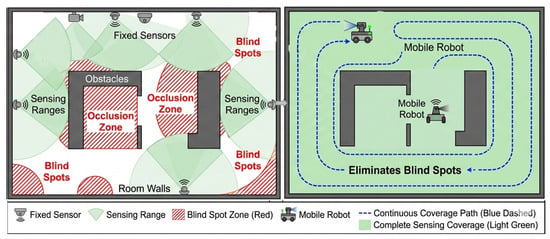
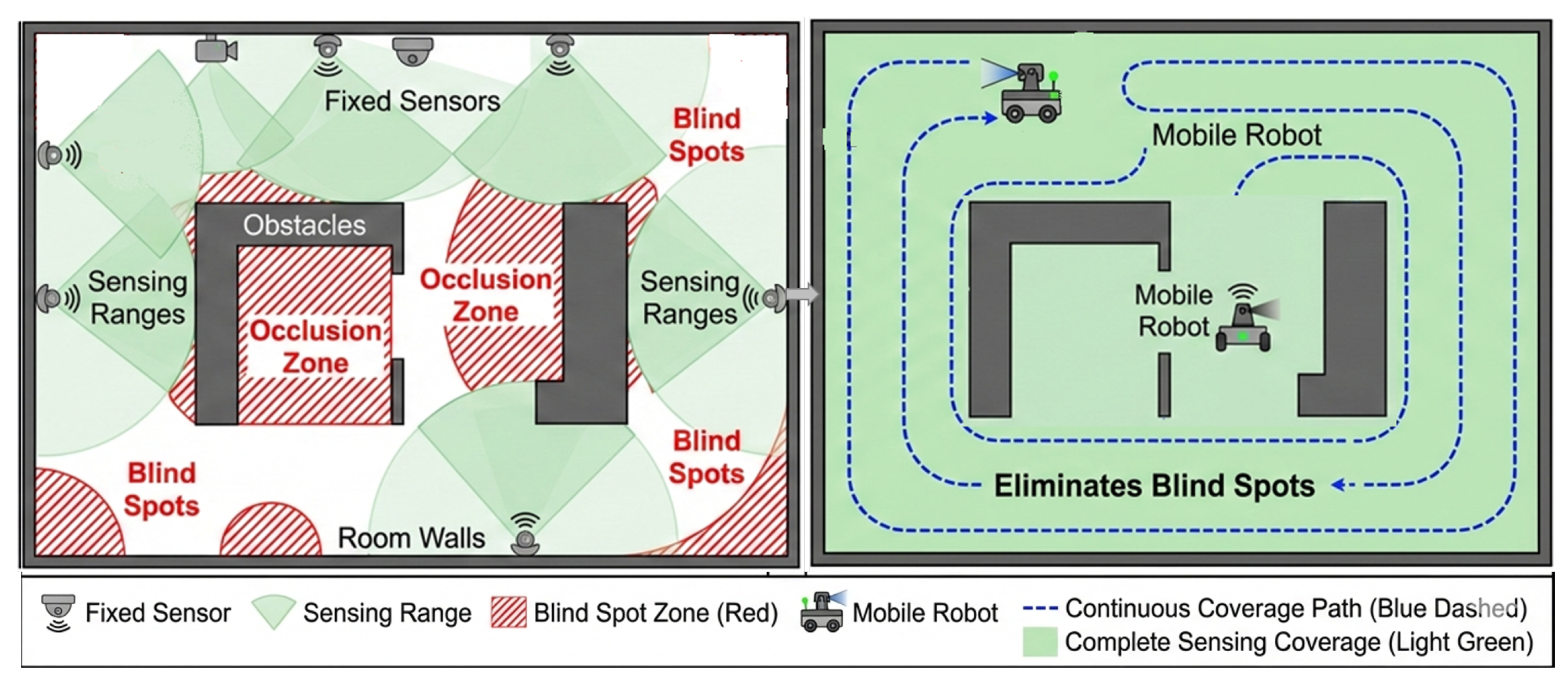
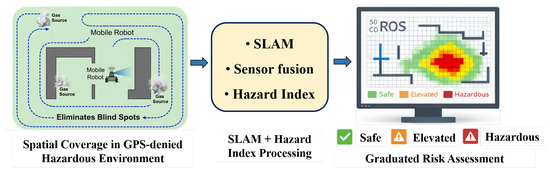
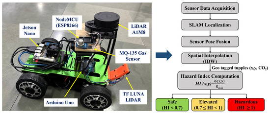
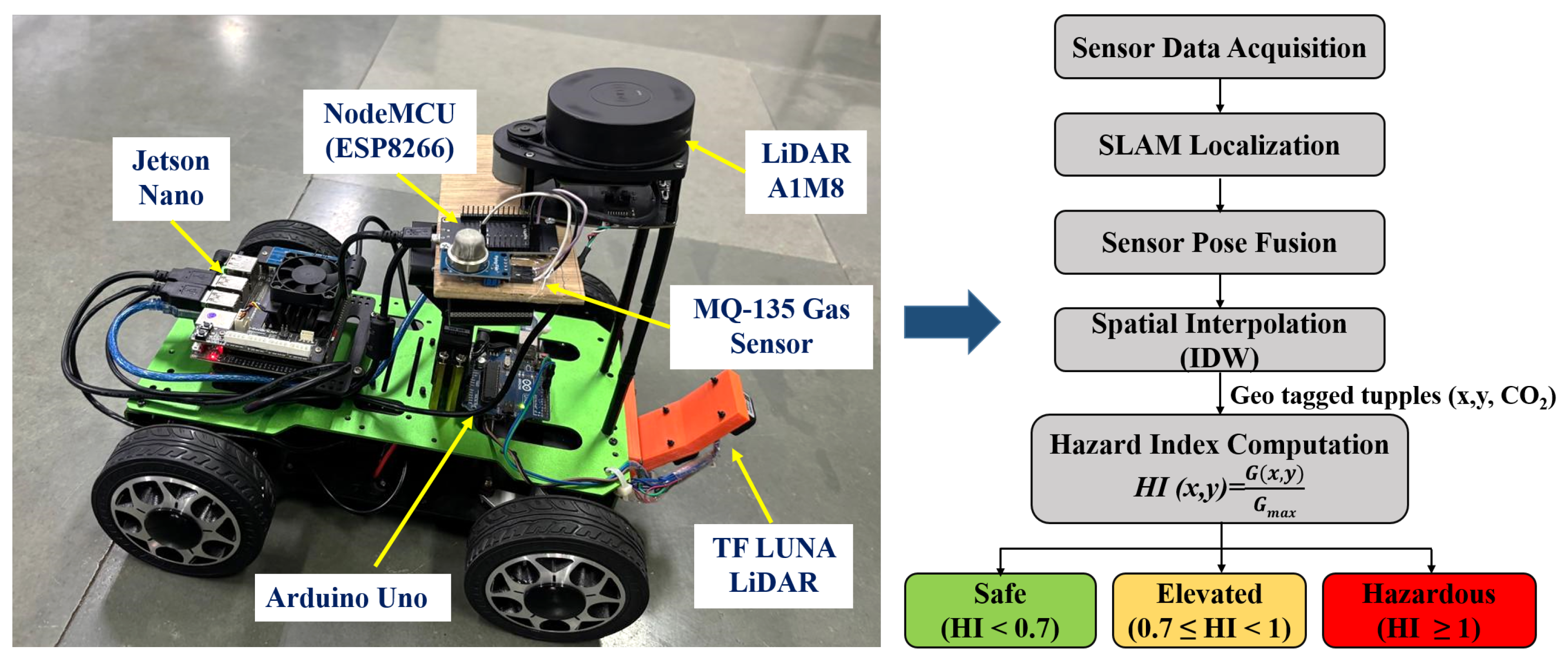
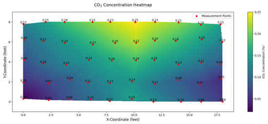
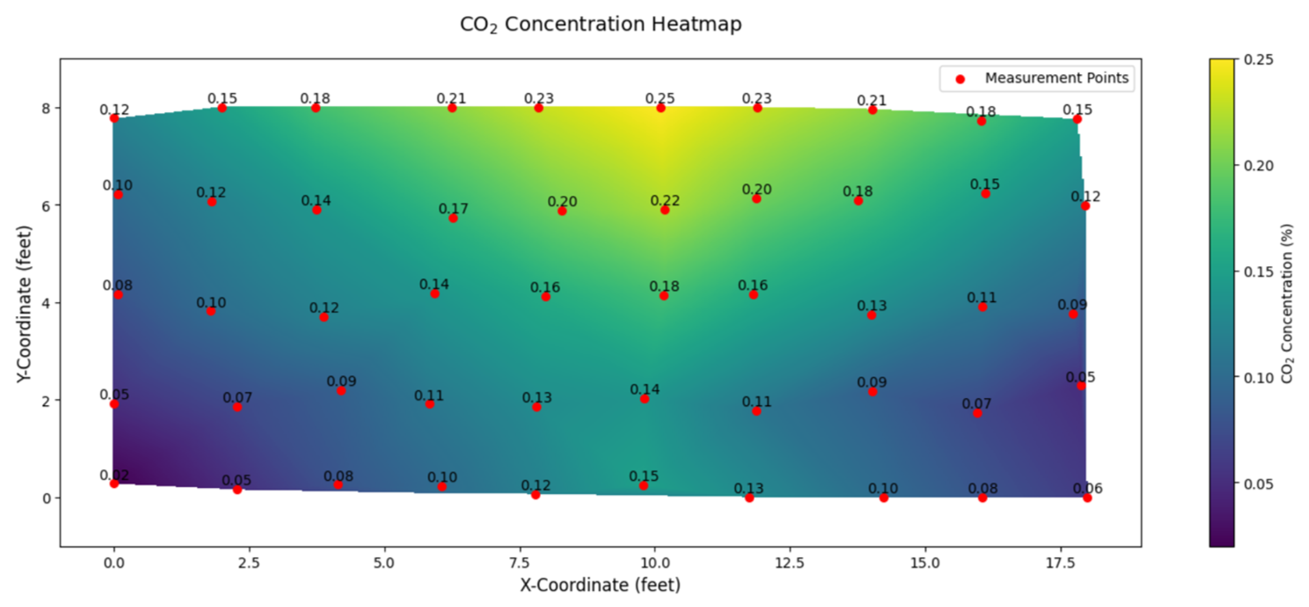
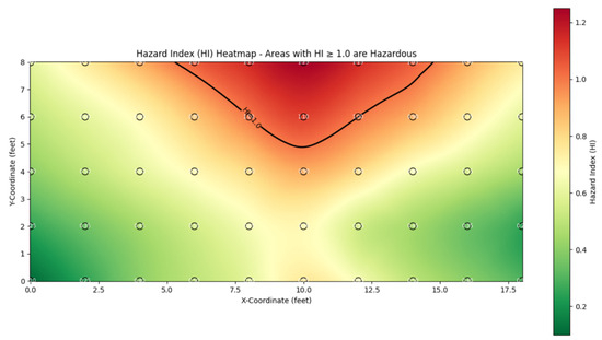
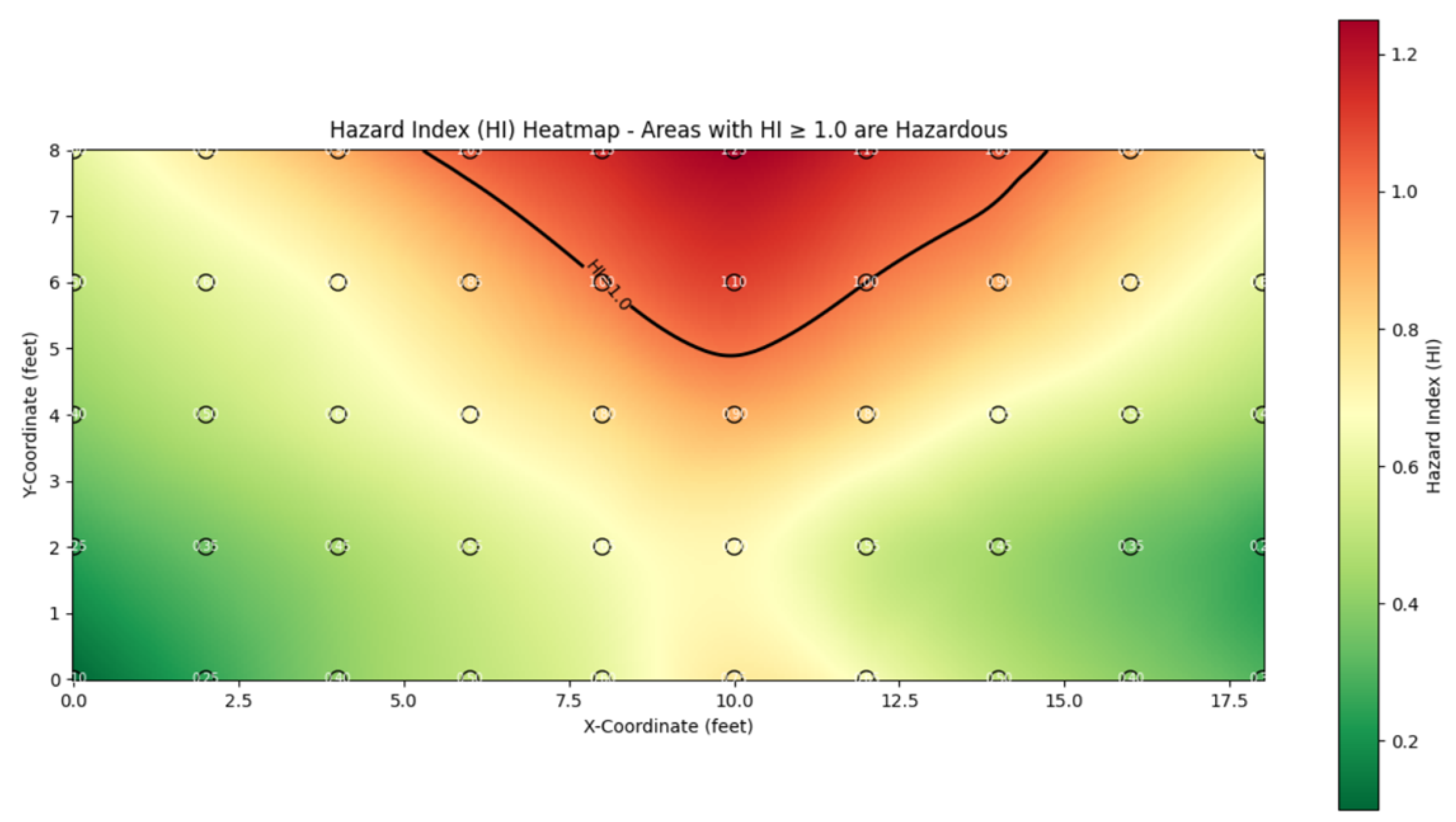
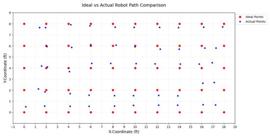
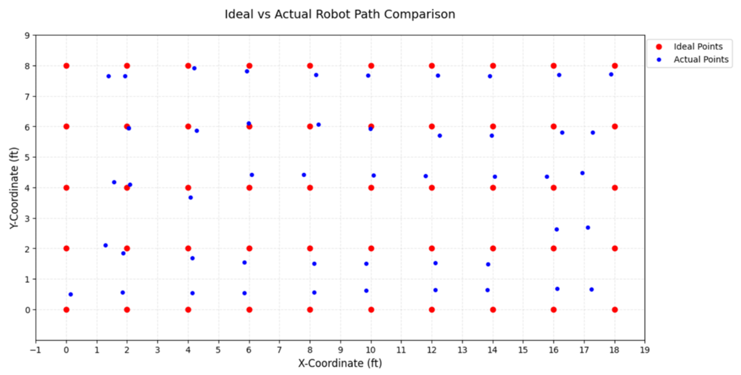
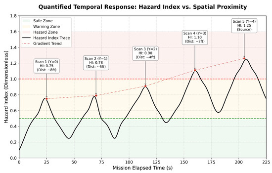
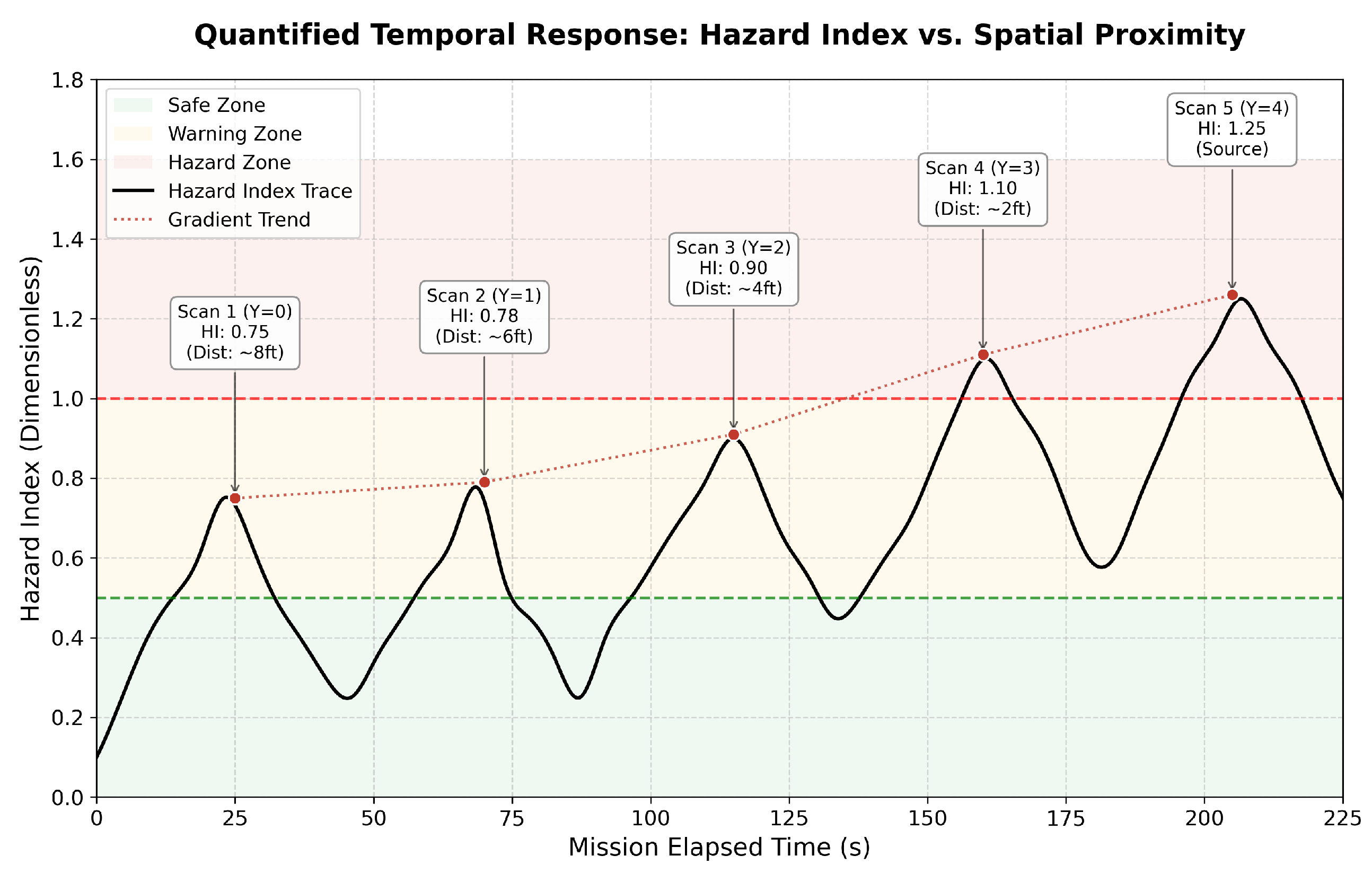

Disclaimer/Publisher’s Note: The statements, opinions and data contained in all publications are solely those of the individual author(s) and contributor(s) and not of MDPI and/or the editor(s). MDPI and/or the editor(s) disclaim responsibility for any injury to people or property resulting from any ideas, methods, instructions or products referred to in the content. |
© 2026 by the authors. Licensee MDPI, Basel, Switzerland. This article is an open access article distributed under the terms and conditions of the Creative Commons Attribution (CC BY) license.