A Multi-Fault Diagnosis System Through Hybrid QuNN-LSTM Deep Learning Models

Abstract

Industrial maintenance and predictive diagnostics constitute fundamental pillars of modern manufacturing that prevent equipment failures, minimize operational downtime, and optimize maintenance costs across diverse industrial environments. Vibration-based fault classification plays an important role in industrial operations, necessitating highly sophisticated diagnostic methodologies. This research addresses these industrial imperatives through a comprehensive investigation of novel hybrid deep learning architectures for vibration-based fault classification. This study introduces a strategic integration of Quadratic Neural Networks (QNNs), which demonstrate superior non-linear feature extraction capabilities on a vibration signal compared to traditional convolutional approaches. A systematic evaluation of seven sophisticated architectures establishes a clear performance hierarchy, with QuCNN-LSTM-Transformer emerging as the optimal model achieving 99.26% average accuracy. All proposed models demonstrate excellence, with test accuracies consistently surpassing 95% across all evaluated scenarios. The data analyzed is emprical utilizing sensor data collected from an experimental rig and shows exceptional performance consistency on CWRU and HUST datasets. This investigation establishes a new paradigm in intelligent diagnostics, offering functional guidance and definitive analysis of hybrid architectures that advance industrial fault classification applications.

1. Introduction

The manufacturing industry has evolved through four industrial revolutions from stream power to digital automation advancing technology [1]. Artificial Intelligence (AI) is fundamental in actualizing Industry 4.0, as it uses data to enable smarter decision making and automation for manufacturing industries, improving production, ensuring consistency, lowering costs, and preventing errors [2]. AI is substantially reshaping Industry 4.0, through predictive machinery maintenance applications, by the early identification of faults and forecasting potential breakdowns, translating directly into significant benefits like increased machine uptime, better cost management, and the effective prevention of operational interruptions [3]. The development and implementation of robust and intelligent machinery Fault Detection and Diagnosis (FDD) methodologies represent a cornerstone of contemporary engineering and industrial asset management. Traditionally, the fault detection and diagnosis system has focused on physics-based modeling and conventional signal processing techniques. Physics-based approaches rely more on the mathematical models, which are susceptible to inaccuracies, whereas signal processing techniques focus on extracting features from sensor data and demand subject expertise. Such methods are effective in identifying distinct signatures of various fault modes but struggle with heterogeneity high dimensionality from sensor data [4].

Machine Learning (ML) has upgraded these FDD strategies by applying algorithms to determine patterns, correlations, and fault signatures from sensor data directly, thereby eliminating the need for manually engineered features [5]. These FDD systems make use of an extensive collection of ML techniques on signal data, such as conventional learning algorithms like Support Vector Machines and Random Forest along with shallow and deep neural networks for classifying known fault types [6,7,8,9]. This integration of machine learning with a machinery fault detection framework helps move industrial systems towards intelligent automation and prognostic health management, enabling comprehensive fault management for enhanced operational efficiency, safety, resilience, and sustainability [10].

Fault diagnostics systems based on signal processing, especially vibrational signals, are an established and still evolving engineering problem. They focus on the analysis of vibrational patterns to precisely detect the operational faults of a machine, specifically rotating equipment [11]. The measured vibration signals of a machine through an accelerometer sensor contain its operating conditions, which can be characterized as vibration signatures, and they are able to provide early warnings of mechanical faults. The critical mechanical faults include various bearing rolling element degradation stages, misalignment, unbalance, cracks, rotor breaks and looseness [12]. Traditionally, the vibration-based fault diagnostics systems have followed signal processing techniques w.r.to time, frequency and time-frequency domains combined with machine learning. The statistical parameters from time domain analysis, utilization of Fast Fourier Transform (FFT) spectra from frequency domain and wavelet transforms, and Short Time Fourier Transform (STFT) from time-frequency domain analysis are the foundations for classifying fault scenarios [13]. Many advanced Deep Learning (DL) approaches are also applied to automate the diagnostic process by enabling the system to learn fault patterns directly from vibration datasets without manual feature extraction as in traditional signal processing but are trained on time-frequency spectrogram images of signals converted through various wavelet transforms [14]. While neural networks are integrated into the system, the raw signal operation is not directly reflected. To enhance this scenario, the recent literature on fault diagnostics systems based on vibrational signals can be seen in the following section.

2. Literature Review

The research on fault diagnosis of vibration signals is majorly characterized by the extensive application of machine learning and deep learning methodologies. A fundamental methodological distinction in these approaches lies in the preliminary processing and feature representation of the raw vibration data, which is typically classified into two predominant paradigms: methods that leverage two-dimensional (2D) transformations, such as converting signals into image or map-based representations, and those that operate directly on one-dimensional (1D) time-series signals. A comprehensive review of the literature for each of these two paradigms is provided in the subsequent subsections.

2.1. Fault Diagnosis Using 2D Image-Based Methods

The following research papers first transformed the 1D time-series vibration data into a 2D image-like format before analysis, typically using a 2D-CNN architecture for fault diagnosis. Ref. [15] et al. introduces a fault diagnosis method that converts signals into RGB images using a Signal-to-RGB Image Mapping (STRIM) technique. These images are then processed by a multichannel multi-scale CNN (MCMS-CNN) for fault classification. The method was tested on the CWRU bearing dataset and achieved a mean classification accuracy of 97.2%. Ref. [16] et al. proposed a deep learning model where one-dimensional vibration signals from the CWRU dataset are converted into two-dimensional images using a Continuous Wavelet Transform (CWT). The model achieved perfect 100% accuracy and maintained performance above 90% even in high-noise environments. Ref. [17] et al. proposed a hybrid CNN and Transformer model where the CWRU data is sampled into spectrograms, which are then used to train the model, and the accuracy was 99.62%. Ref. [18] et al. proposed a method that first uses Local Maximum Synchro squeezing Wavelet Transform (LMSWT) to get a two-dimensional time-frequency image. This image is then fed to a CNN that incorporates a channel attention mechanism (SE-MSCNN), which is validated on the CWRU, Paderborn, and HUST datasets, achieving an accuracy that exceeds 98.06%. Ref. [19] et al. proposed a methodology by converting signals into Log Mel-spectrograms, which is then run on a VGG model, achieving an accuracy above 92.11% for the CWRU dataset and over 99.25% for the PU dataset.

2.2. Fault Diagnosis Using 1D Signal-Based Methods

The following research papers use the time-series vibration data directly as input. Ref. [20] et al. proposed a method named S-AlexNet, a lightweight convolutional neural network (CNN) validated on the CWRU dataset and a self-built experimental dataset. The S-AlexNet model demonstrated high accuracy and efficiency, achieving 94.40% on the CWRU data and 99.84% on the self-built data. Ref. [21] et al. compared the performance of CNN and Long Short-Term Memory (LSTM) models for bearing fault diagnosis on the CWRU dataset, which focused on how hyperparameter tuning can enhance accuracy and robustness against varying Signal-to-Noise Ratios (SNRs). The CNN achieved an accuracy of 97.96%, whereas the LSTM model only reached 94.46%. Ref. [22] et al. presented a diagnostic model with a CNN and LSTM validated on the CWRU dataset, with an accuracy of 99.83%. Ref. [23] et al. proposed a simplified Wide Convolutional Neural Network (WDCNN) with a Random Forest (RF) classifier for bearing fault diagnosis on the CWRU dataset, which resulted in 99.6% accuracy. Ref. [24] et al. presented a Convolutional Long-Short-Term-Memory Recurrent Neural Network (CRNN) that was validated on two datasets, CWRU and IMS, with overall classification accuracies of 99.77% for the CWRU dataset and 97.13% for the IMS dataset. Ref. [25] et al. proposed a hybrid model that combines CNN and LSTM and was validated on the Jiangnan University dataset, with an accuracy of 95% on single-load conditions. Ref. [26] et al. proposed a multitask deep learning model that merges a CNN and LSTM on the HUST motor bearing dataset, which resulted in both fault diagnosis and classification accuracy.

Across both 1D signal-based and 2D image-based paradigms, firstly, common research was focused on the benchmark dataset, with the CWRU and, to a lesser extent, HUST datasets being predominant. While this is the basis for comparison, it also highlights a critical need for more diverse and challenging datasets to ensure broader model generalization. Secondly, researchers address the critical challenges of noise robustness and performance under varying load conditions. A key distinction in their methodology remains, however; while many deep learning models in both 1D and 2D categories aim for automated, end-to-end feature learning directly from the data, a subset of 1D techniques continues to leverage traditional, explicit feature engineering steps. Addressing these, the primary objectives of this work are defined as follows:

• To develop a generalizable fault diagnosis model that must accurately identify a comprehensive range of fault conditions, including both single and compound (simultaneous) faults across diverse datasets.
• To design an end-to-end learning architecture that directly processes raw 1D time-series signals, which will enable the model to learn and capture temporal dynamics of fault signatures automatically, thereby eliminating the need for manual feature extraction and selection.

3. Proposed Methodology

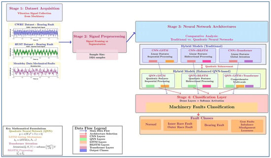
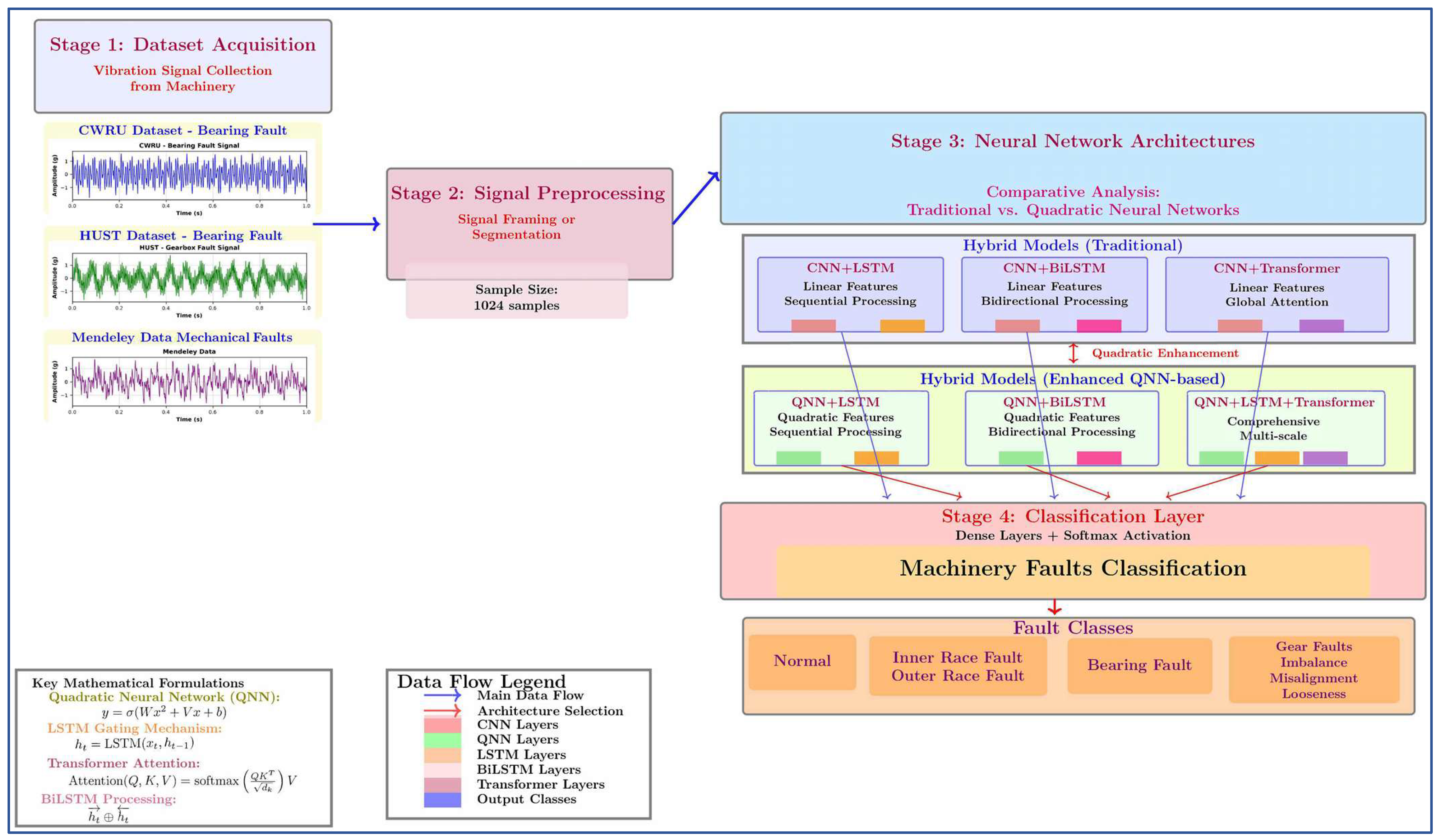
The methodological framework for this study is structured as a systematic, multi-stage process, as shown in Figure 1. The procedure commences with the acquisition of raw time-series vibration data from three heterogenous repositories. The development phase employs a comparative architectural analysis between traditional hybrid models (CNN-LSTM, CNN-BiLSTM, CNN-Transformer) and novel quadratic neural network-enhanced variants (QuCNN-LSTM, QuCNN-BiLSTM, QuCNN-LSTM-Transformer), where the quadratic layers introduce non-linear quadratic feature transformations to capture complex machinery dynamics that conventional linear approaches may inadequately represent. The systematic preprocessing stage implements signal segmentation with 1024-sample segments, while the classification layer utilizes dense neural architectures with softmax activation for multi-class fault categorization, encompassing normal conditions, bearing defects (inner race, outer race, ball faults), and additional mechanical anomalies including gear faults, imbalance, misalignment, and looseness.

Figure 1. Vibration-based fault detection workflow.

The architectural design demonstrates the methodology through its incorporation of attention mechanisms via transformer components and bidirectional temporal modeling through BiLSTM layers, making this a comprehensive solution for intelligent condition monitoring in industrial machinery systems. Each step implemented is described in the following subsections.

3.1. Datasets

To implement the primary objective of our work, three benchmark datasets are considered to address the diverse datasets and comprehensive range of fault conditions with both single and compound faults. Although industrial production scale does not directly apply to the generated signals data from electromechanical test rigs, these datasets are standardized for real world machinery. The experimental setup is on continuous rotating machinery with manufacturing environments for evaluating bearing components driven by motors. The scale and complexity of diagnostic challenges are based on the operating states and severity. The empirical data collected is high frequency time series vibration data from accelerometer sensors on a physical experimental test rig for reliable diagnostics closer to industrial reality. The technical specifications and empirical data descriptions of each dataset are shown below.

3.1.1. Case Western Reserve University Dataset (CWRU) [27,28]

The first dataset considered in this study is the Case Western Reserve University (CWRU) 48 kHz dataset. It has 47 distinct fault data files and four additional normal baseline files, all provided in the MATLAB 5.0 (.mat) format. Each file is a raw time-series signal with a substantial number of samples at a sampling rate of 48 kHz, typically over 480,000 data points, primarily from an accelerometer at the motor’s drive end. The experimental setup was running a 2 hp motor with four distinct motor loads (0 to 3 hp) and three types of artificially induced bearing defects: inner race, ball, and outer race faults in three different diameters (0.007, 0.014, and 0.021 inches). For a model to learn the relevant diagnostic patterns effectively and to maintain consistency, all files of 48 KHz signals are divided into 420 smaller segments of 1024 samples without overlap to generate hundreds of individual training instances, which is essential for training deep learning models.

3.1.2. HUST Bearing Dataset [29,30]

Another dataset considered in this study is the HUST bearing dataset, which consists of 99 vibration signals from five bearing types: bearing 6204 to 6208. It encompasses six classes of defects, including individual inner, outer, and ball cracks as well as their two-fault combinations. Data was captured under three distinct load conditions (0 W, 200 W, and 400 W), and each vibration signal was sampled for 10 s at a high rate of 51,200 Hz to capture detailed signal changes. The experiments were run on a 750 W induction motor test bench with a powder brake to simulate loads and an accelerometer to measure vertical vibration.

3.1.3. Mechanical Faults in Rotating Machinery Dataset from Mendeley [31]

The third dataset considered in this study is the mechanical faults in rotating machinery dataset from Mendeley data, with four fundamental operational conditions: a baseline normal state and three common fault scenarios—unbalance, misalignment, and mechanical looseness. Data was collected from a dedicated test rig, which included a motor run for 20 distinct test sets, with five repetitions for each of the four conditions at four accelerometer positions. The two accelerometer positions are at pulley on vertical (VSCP) and horizontal sides (HSCP), and the other two are at disk vertical (VSOCD) and horizontal opposite sides the coupling (HSOCD). There are a total of 420 signals in .npy (NumPy data array) format from each side where each signal is sampled at 25 kHz, resulting in 25,000 data points per signal file, which consists of 8400 signals per accelerometer. The 420 signals data is combined and saved as a single compressed archive named array .npz file, and all signal files are arranged into folders as per test accelerometer positions with 5 test runs. Each file is renamed to indicate the test run, fault case, and the accelerometer position. The file name 1_Misalignment_HSCP signifies that it is first run and misalignment fault and horizontal side of the coupling pulley accelerometer position. The data is renamed for all files for each test run and is given as input to the models. For a model to learn the relevant diagnostic patterns effectively and to maintain consistency, all signals are divided into smaller segments of 1024 samples without overlap to generate hundreds of individual training instances, which is essential for training deep learning models. The technical specifications of these three datasets are depicted in Table 1.

Table 1. Technical specifications and empirical data of three experimental bearings used in this study.

Dataset	CWRU [27]	Mendeley [31]	HUST [29]
Source	CWRU Bearing Data Laboratory Center	-	Hanoi University of Science and Technology Laboratory Center
Acquisition Setup	Experimental Test Rig	Experimental Test Rig	Experimental Test Rig
Motor Model	2 hp Reliance Motor	3 Ph Induction Motor	750 W Induction motor
Accelerometer	PCB 353B33	PCB 325C33	PCB 325C33
Bearing	SKF 6205-2RS JEM	Bearing 1205	KG 6204 to 6208
Frequency	48 kHz	25 kHz	52 kHz
Format	.mat	.npy	.mat
No. of files	47	20	99
Faults	Bearing Inner Race Outer Race	Looseness Misalignment Unbalance	Bearing Inner Race Outer Race

3.2. Classification Models

To implement the second objective of our work, hybrid deep learning models are considered to classify the diverse datasets and comprehensive range of fault conditions with both single and compound faults. The description of each model and architecture is shown in the following subsections.

3.2.1. CNN-Based Hybrid Models

CNN-LSTM

The first model implemented in this work combines convolutional and LSTM layers to process signal sequential data by CNN and discerning long-range temporal dependencies. In essence, the CNN-LSTM paradigm works by first employing the CNN to act as a hierarchical feature extractor of signals and LSTM to remember these temporal dependencies [32,33,34]. Initially, the model takes one-dimensional signal inputs of shape 1024 × 1 vector (x) employed by convolutional layers to capture spatial patterns as it effectively transforms raw signals into a more abstract, temporal format [34]. The subsequent integration of LSTM layers are these recurrent units designed to retain information and overcome the vanishing gradient problem inherent in simpler recurrent networks [35]. The sequences are then transformed via an LSTM layer, expressed as in Equation (1), which adeptly models sequence dependencies by learning patterns of signals across time. Throughout the layers, strategically applied dropout mechanisms provide crucial regularization and ReLU activation, defined within layers by x_relu= relu(x), ensuring non-linearity and efficient gradient propagation. This multi-layered approach is suitable as it follows a hierarchical learning process, where initial layers detect features and deeper layers synthesize these into more complex representations [36].

$$h_t=LSTM\_Layer\left(x_{conv}\right)$$

(1)

The model accepts a 1D signal (x) with a shape of (1024, 1), representing 1024 timesteps with a single feature. There are two convolutional blocks. The first Conv1D layer has 64 filters, and the second has 128 filters, both with a kernel size of 5, and each is followed by BatchNormalization, MaxPooling1D. These layers apply filters to detect local patterns and features within the signal and to stabilize learning by normalizing the activations. MaxPooling1D down-samples the feature maps, reducing computational complexity. This CNN part acts as a powerful feature extractor, transforming the raw signal into a higher-level representation that is more informative for the subsequent recurrent layer represented as (x_conv). The LSTM layer consists of an LSTM unit with 128 cells that learns signal long-term dependencies and serves a hidden state output (h_t). The input is the feature map from the CNN part (256, 128). The output is a vector of size 256. This layer is critical for modeling the temporal dynamics of the features extracted by the CNN and to understand the sequence of patterns, which is essential for classifying signal data. Next, two Dense layers with 128 and 64 units respectively act as a classifier, taking the features from the LSTM and learning non-linear combinations of them. They map the learned sequential features to a space where the classes are separable. A final Dense layer with num_classes and a ‘softmax’ activation function produces the final classification result.

CNN-BiLSTM

The CNN-BiLSTM model elevates the temporal pattern recognition capabilities by incorporating bidirectional sequence learning by analyzing information in both forward and backward directions of each data point. The initial convolutional layers are vital in this process, performing essential feature extraction; their operation follows the expression x_conv1D = relu(conv1D(x)). This setup allows the model to leverage CNN for initial spatial detection, providing compressed representation of the input, while the subsequent BiLSTM layers perform forward and 1 backward pattern analysis [37,38], defined as,

$$h_t=BiLSTM\_layer\left(x_{conv}\right)$$

(2)

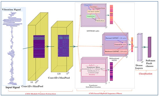
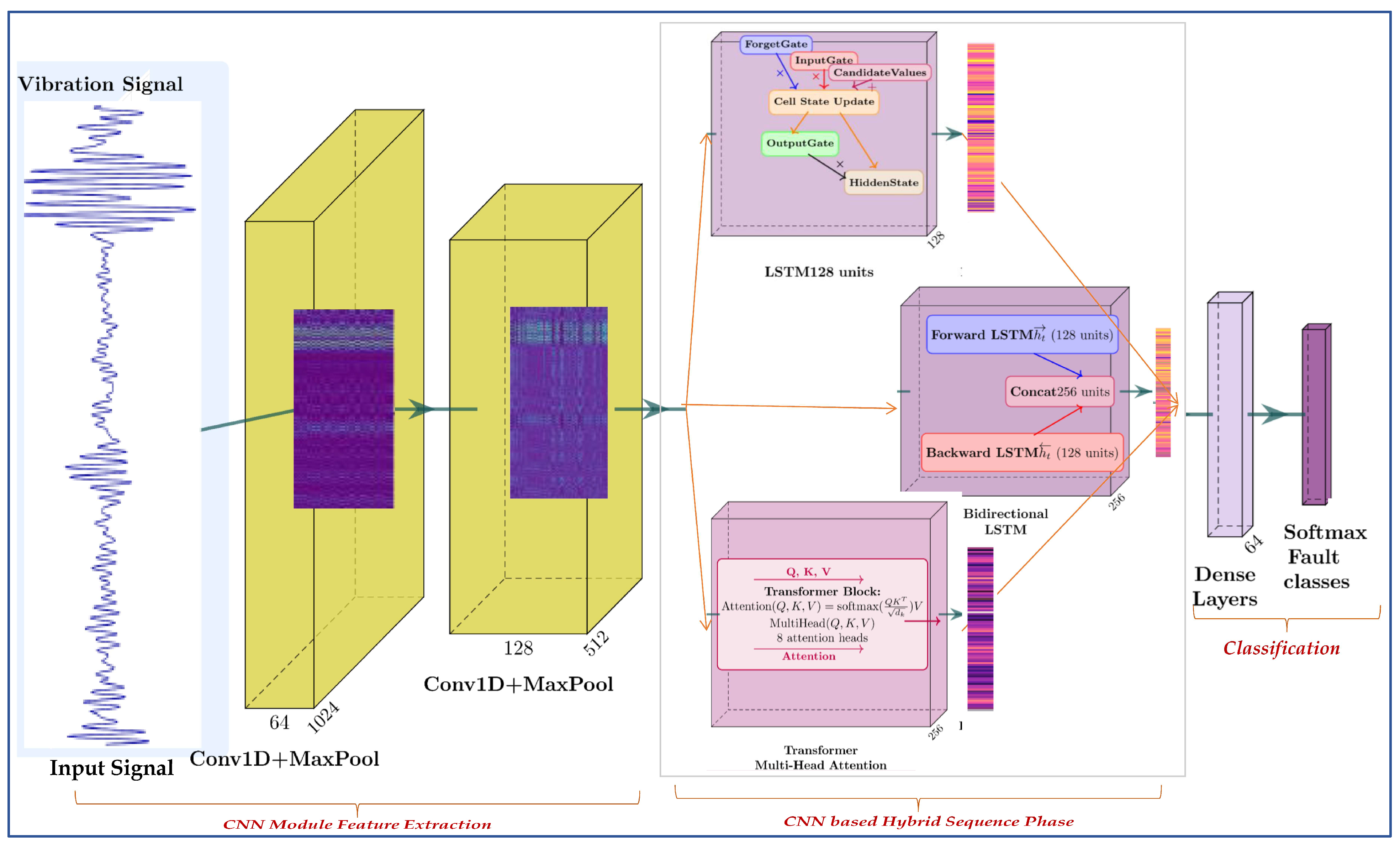
The bidirectional flow captures dependencies that might be missed by a unidirectional approach, offering a more complete picture of the signal sequence. The combination effectively transforms raw signals into a representation that leads to more informed predictions and classifications [39]. A Conv1D layer (x_conv) with 64 filters scans the input signal (1024, 1) to detect 64 distinct patterns. MaxPooling1D then down-samples the sequence by half, reducing computational load. This block repeats with 128 filters to learn more complex features, resulting in a feature of 256 sequences. The bidirectional wrapper with two LSTM networks—one forward and one backward—process the features and outputs (h_t), which is crucial for differentiating complex signal classes. This layer returns a 256-dimensional vector forwarded to a series of dense layers to map to the final class probabilities. The model architecture is depicted in Figure 2.

Figure 2. Detailed architecture of CNN-based hybrid models.

CNN-Transformer

The CNN-Transformer model represents a paradigm shift in signal processing by integrating the local feature extraction of convolutional neural networks with the global attention mechanism of transformer architectures, enabling comprehensive analysis of both spatial and temporal dependencies in vibration signal data. This hybrid approach leverages the strengths of CNNs for hierarchical feature learning while employing transformer blocks to capture signal long-range dependencies through self-attention mechanisms. Initially, the model processes one-dimensional signal inputs of shape 1024 × 1 through convolutional layers that extract localized patterns and features, followed by max-pooling operations. The subsequent transformer block implements multi-head self-attention mechanisms, mathematically defined as,

$$Attention\left(Q,K,V\right)=softmax\left({\displaystyle \frac{QKT}{\sqrt{d_k}}}\right)V$$

(3)

where Q, K, and V represent query, key, and value matrices respectively [40]. The multi-head attention with 8 attention heads allows parallel processing, enhancing the model’s ability to capture diverse signal characteristics simultaneously, which contributes to accurate classification.

3.2.2. QuCNN-Based Hybrid Models

The proposed model utilizes the quadratic function to enhance and extract fault features, as the mechanical faults prohibit non-linear dynamics of the machinery impacting the vibration amplitude. This captures the physical severity and degradation of the faults than linear approximations of the model. The proposed models with quadratic function implementation used in this study are described in the following subsections.

QuCNN-LSTM

This is a paradigm-shifting model integrating custom Quadratic Neural Network (QuNN) layers to activate sophisticated non-linear transformations, marking a fundamental break from conventional network designs. This approach extends the expressive power of neural networks beyond simple linear combinations of inputs, allowing for the capture of more intricate relationships within the data. The standard layers are replaced with quadratic neurons, expressed as,

$$y=\sigma (W{x}^2+Vx+b)$$

(4)

where, x is an input signal, W, V, represents weights, b is bias and y is the output of quadratic layer. This formulation enables the model to inherently learn second-order relationships and interactions between features, which can be crucial for understanding complex and high-dimensional data signals. Remarkably, with reduced parameters, the QuCNN-LSTM maintains considerable expressive power, optimizing computational resources while boosting analytical depth. The LSTM layers regulate information flow, enabling the learning of long-term patterns [41], defined as

$$h_t=LSTM\_layer\left(x_{qnn}\right)$$

(5)

The QuCNN layers contribute to a richer feature representation space, allowing the LSTM to operate on more highly informative signal inputs [42]. The unique quadratic operation provides a novel mechanism for information processing. The model takes raw fault signals data as input (1024, 1), where 1024 represents the number of data points in each signal sample. The first QConv1D with 32 filters is applied to the signal with ‘relu’ maxpooling to down-sample the feature, resulting in the dimensions (126, 32). A second Qconv block with 64 filters learns more complex and higher-level feature combinations from the initial features of signals. The output is a sequence of feature vectors represented as (x_qnn) processed by the LSTM layer. This layer contains 128 LSTM units that process the sequence of 62 feature vectors (each of size 64) with 40% dropout ratio for regularization with a dense layer for classification, introducing higher-order feature interactions. The model learns both linear and quadratic relationships between the features extracted by the LSTM, potentially capturing more complex decision boundaries. It has 128 units and uses a ‘relu’ activation. A standard fully connected layer outputs a probability distribution over the fault classes possible categories.

QuCNN-BiLSTM

The QuCNN-BiLSTM model utilizes the power of quadratic transformations with bidirectional sequence learning, which enables the model to simultaneously uncover non-linear relationships within features and capture dependencies across both past and future contexts in signal data [43]. Its bidirectional sequencing provides dual-dimensional pattern analysis, and its enhanced by the quadratic dynamics, as defined in Equation (4). The quadratic layers imbue the model with capacity to learn second-order features, which can be critical for understanding complex data signal behaviors often overlooked by linear models. The BiLSTM component process sequences in both forward and backward directions, which provides deeper temporal correlations and more non-linear representations particularly effective for highly variable signal data.

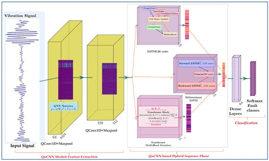
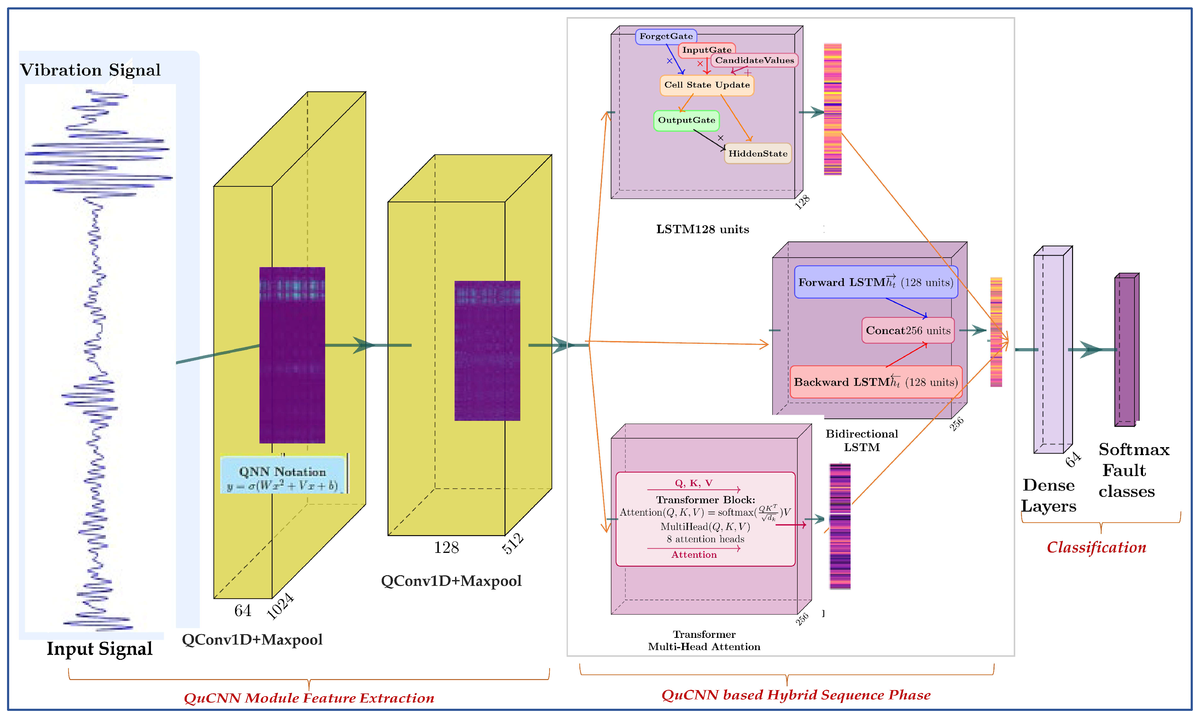
The model takes raw fault signals data as input (1024, 1), where 1024 represents the number of data points in each signal sample. The first QConv1D with 32 filters is applied to the signal with max-pooling to down-sample the features and to capture broad, low-level patterns. The second QConv1D layer uses 64 filters to learn higher-level features. A BiLSTM uses two separate LSTM networks (each with 128 units) and concatenates their output (256) by processing the sequence in both the forward and backward directions simultaneously. The custom Quadratic Layer allows the model to learn second-order relationships and features, which include both a standard linear and quadratic transformation of its input features, leading to a better decision boundary. The dense layer takes the (256) vector from the BiLSTM and produces a final probability fault class, as depicted in Figure 3.

Figure 3. Detailed architecture of QuCNN-based hybrid models.

QuCNN-Transformer

The QuCNN-Transformer model, a self-attention mechanism with quadratic layers, provides both global contextual understanding and enhanced non-linear feature processing designed to overcome the limitations of traditional sequential models by processing entire sequences in parallel, thereby improving efficiency for long dependencies. It adopts a multi-head attention framework, a core component of the Transformer, which is further augmented by the potent quadratic power, allowing the model to weigh the importance of all parts of the input signals simultaneously for each data point [35]. The model predominantly focuses on long-range dependency analysis and is executed through its self-attention mechanism as in Equation (3). The quadratic layers then infuse the attention-derived non-linear capabilities to form correlations from the attended features of varied signal data. The Transformers parallel processing capability makes it significantly faster for long sequences [37]. The QuCNN layers, in turn, can model subtle interactions between features discovered by the attention mechanism.

QuCNN-LSTM-Transformer Model

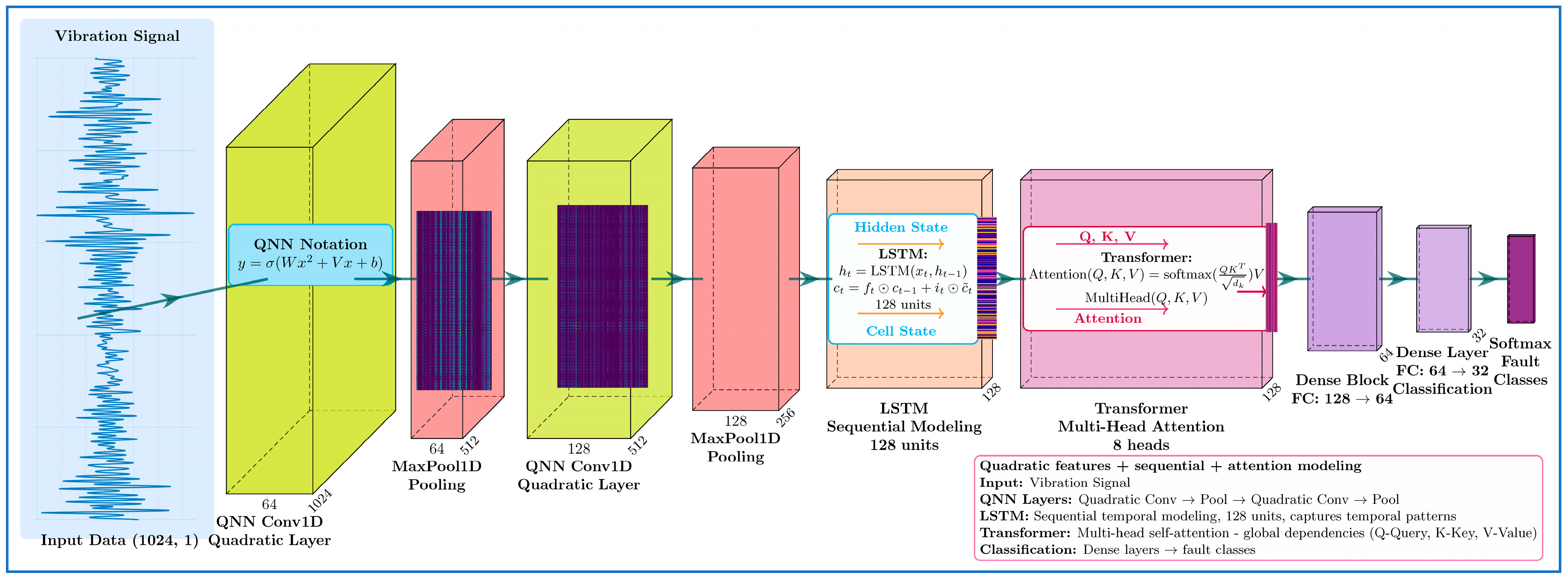
This architecture represents a hierarchical deep learning paradigm that integrates quadratic feature transformation, sequential temporal modeling, and global attention mechanisms for enhanced vibration-based fault detection. The quadratic neural network component performs sophisticated non-linear feature extraction through second-order polynomial operations, as in Equation (4), enabling the capture of complex quadratic relationships inherent in mechanical fault signatures while maintaining computational efficiency [44].

Sequential processing through LSTM layers addresses temporal dependencies via gating mechanisms, effectively modeling long-term information flow across extended vibration sequences. The transformer module applies self-attention mechanisms to LSTM outputs, creating comprehensive representations that capture both local quadratic relationships and global temporal dependencies. This tri-layered architecture excels at multi-scale temporal analysis, where progressive feature refinement through each specialized component contributes to superior fault detection performance in complex mechanical systems.

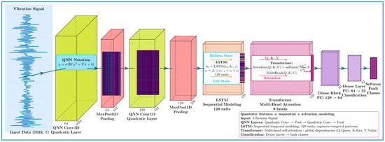
The hierarchical design enables the model to simultaneously process short-term quadratic interactions, medium-range temporal patterns, and long-range global dependencies, making it particularly effective for sophisticated fault diagnosis scenarios. This effectiveness of the model is demonstrated where the raw vibration input signal is initiated to the process. The Quadratic convolution layer maps the signal into 64-dimensional feature space, and by the transformer stage, the self-attention mechanism adds weights to the faults. This ensures each fault category is unique. Figure 4 illustrates the flow of the proposed diagnostic system, where the raw vibration signal from the CWRU bearing dataset is given as input. The input signal features passed through quadratic convolution filters are learnt, and the feature maps and learning probabilistic diagnostic outputs are shown.

Figure 4. Detailed architecture of QuCNN-LSTM-Transformer model.

4. Experimentation Results

An advanced deep learning investigation was conducted on a high-performance desktop system, and the processing power was driven by a 12th Gen Intel Core i5-12400F CPU (Intel, Santa Clara, CA, USA). This x64-based PC was configured for intensive computational tasks, leveraging a dedicated, high-performance NVIDIA GeForce RTX 4060 Ti (NVIDIA, Santa Clara, CA, USA) graphics processing unit that possesses a substantial 16.0 GB of dedicated GDDR VRAM, enabling it to handle large datasets and complex models essential for deep learning and high-resolution texturing. The memory architecture is further augmented by access to 15.9 GB of shared memory, bringing the total addressable GPU memory to 31.9 GB within a Jupyter Notebook version 7.2.2 environment to accelerate model training. The experimental framework was built upon TensorFlow 2.x with Keras API for rapid prototyping and streamlined model development. A robust data preprocessing pipeline was established using NumPy and Pandas for numerical transformations and data manipulation, respectively.

The dataset files were first loaded and split into distinct training and testing based on two-stage sampling prior to the segmentation process, preserving the integrity of the data files to prevent data leakage. In stage 1, the samples are split in 85% (train–validation) and 15% for testing by isolating it first. At stage 2, the train–validation is split into 70% train and 15% validation. The train–test split samples for the datasets used are shown in the following Table 2.

Table 2. Train–test samples of the datasets.

Dataset	Filename	Total Files	Total Segments	Train (70%)	Val (15%)	Test (15%)
CWRU	7	23	9660	7140	1680	1680
	14	16	6720	5040	840	840
	21	23	9660	7140	1680	1680
	all	62	26,040	19,320	4200	4200
HUST	4	16	6720	5040	840	840
	5	16	6720	5040	840	840
	6	16	6720	5040	840	840
	7	16	6720	5040	840	840
	all	64	26,880	20,160	3360	3360
Mendeley	HSCP_Test	20	201,600	141,120	30,240	30,240
	VSCP_Test	20	201,600	141,120	30,240	30,240
	HSOCD_Test	20	201,600	141,120	30,240	30,240
	VSOCD_Test	20	201,600	141,120	30,240	30,240
	all	80	806,400	564,480	120,960	120,960

4.1. Experimental Setup and Hyperparameters

To ensure transparency of the proposed methodology, the model was trained on standard configurations. The network was optimized using the Adam optimizer, well suited for hybrid architectures due to its adaptive learning capabilities, with early stopping to prevent overfitting. The complete architectural hyperparameters are detailed in Table 3 below.

Table 3. Training hyperparameters.

Parmeter	Value	Justification
Optimizer	Adam	Adams adaptive learning navigates the mechanical fault impacts
Learning rate	0.001	Ensures steady convergence preserving high frequency signal features
Batch size	32	Enhances unseen fault conditions
Max Epochs	50	Sufficient iterations to learn fault patterns
Loss function	Categorical Cross entropy	Fault classes
Dropout rate	0.3	To learn distinct fault features

4.2. CWRU Dataset Results

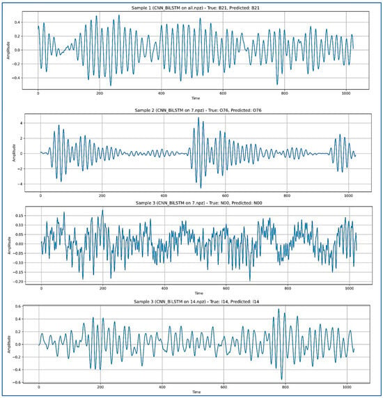
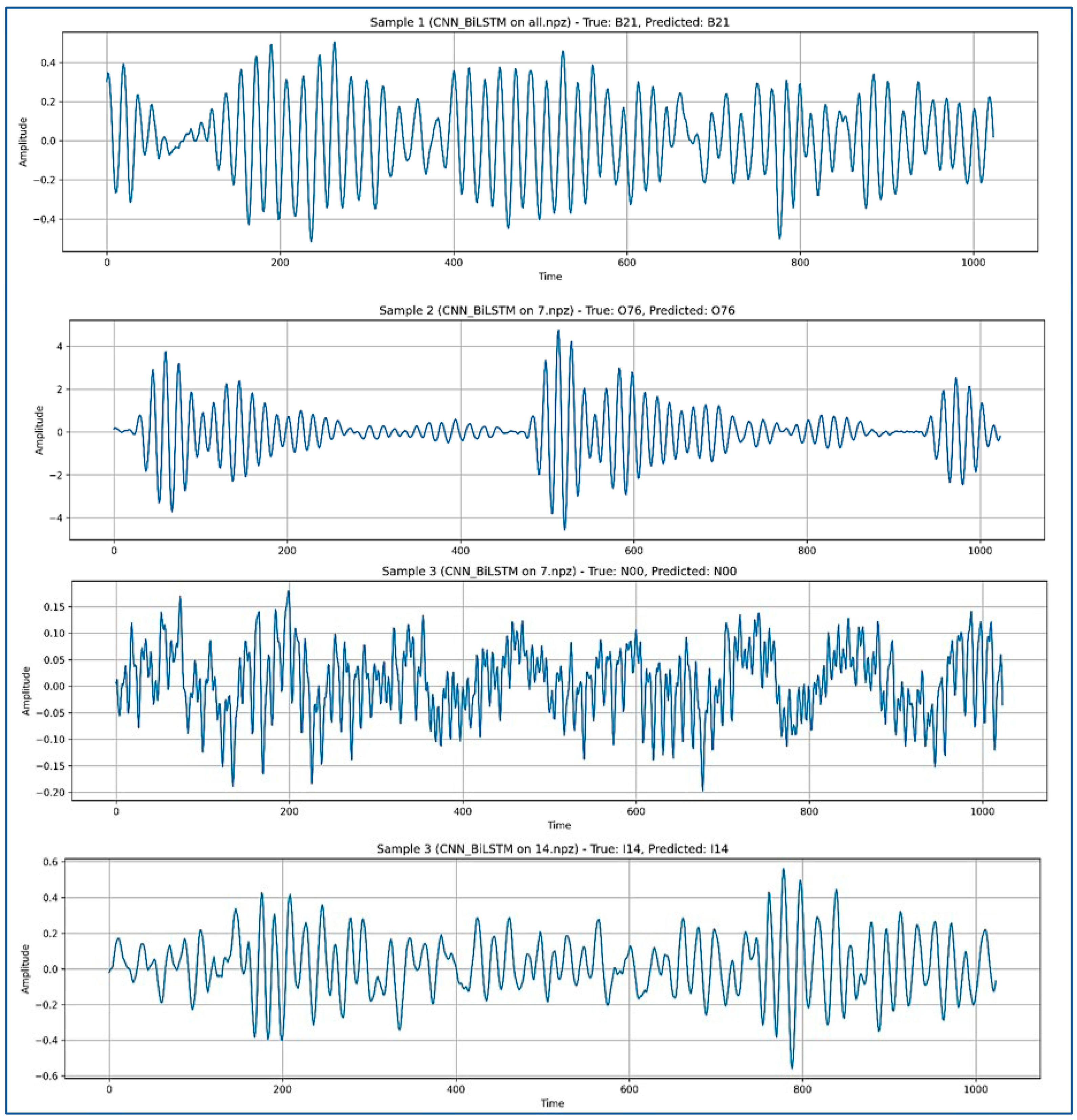
The results show a comparative analysis of hybrid deep learning models on a faults classification, evaluated across four distinct cases categorized by fault diameter (7, 14, and 21 mils) of the CWRU dataset, as shown in Table 4. Every architectural configuration surpasses the 96% accuracy threshold, affirming the suitability of deep learning for capturing complex patterns within vibration signal data. When paired with sequential modules, the QUCNN-based models consistently demonstrate performance that is superior to their CNN-based models, which establishes the QUCNN as a viable alternative for signal feature extraction in modeling non-linear relationships of signal data. Figure 5 shows the samples of the vibration signals tested true for bearing, outer and inner race faults along with normal signal of CWRU data.

Table 4. Summary of CWRU dataset results.

CWRU Dataset	7 Mils		14 Mils		21 Mils		All
Model Accuracy	Val	Test	Val	Test	Val	Test	Val	Test
CNN + LSTM	100	100	99.38	99.18	99.93	99.73	98.59	98.71
CNN + BiLSTM	99.93	100	99.49	99.38	99.93	100	98.73	98.75
CNN + Transformer	99.86	99.93	99.38	99.38	99.86	99.45	97.15	96.91
QNN + LSTM	99.93	99.93	99.44	99.37	99.93	99.93	96.94	96.68
QNN + BiLSTM	99.93	100	98.56	98.15	99.93	100	98.76	98.71
QNN + Transformer	99.86	99.93	99.38	99.38	99.86	99.45	97.15	96.91
QNN + LSTM + Transformer	100	100	99.59	99.49	100	99.93	98.76	98.94

Val—Validation.

Figure 5. CWRU data’s sample signals predicted by CNN_BiLSTM model.

The choice of the sequential processing unit also yields good performance variations, where the BiLSTM variants achieve perfect 100% test accuracy in multiple scenarios, such as the CNN-BiLSTM and QUCNN-BiLSTM models on the 7 and 21 mils datasets. The QUCNN-LSTM-Transformer architecture represents a sophisticated fusion of the novel QUCNN feature extractor, the proven sequential modeling of LSTM, and the powerful attention mechanism of the Transformer. This configuration consistently delivers stable results across all test conditions. It achieves the highest test accuracy on the ‘14 mils’ subset case, with 99.49%, where the other models showed slightly reduced performance. Even more significantly, it attains the top score of 98.94% on the ‘all’ dataset case, demonstrating its robustness with many fault severities.

4.3. HUST Dataset Results

The empirical investigation demonstrates exceptional diagnostic performance across hybrid deep learning architectures on the HUST dataset. All configurations systematically exceed the 96% accuracy threshold, achieving near-optimal results, with test accuracies spanning 99.88% to 100%. This exemplary performance validates the profound analytical capacity of deep learning frameworks in deconstructing complex vibrational phenomena. The architectural analysis reveals sequential processing units as pivotal performance determinants. Bidirectional Long Short-Term Memory (BiLSTM) implementations, particularly CNN-BiLSTM and QUCNN-BiLSTM variants, consistently achieve statistical perfection. The bidirectional temporal processing paradigm enhances contextual comprehension of embedded fault signatures within time-series architectures. The QUCNN-LSTM-Transformer configuration exemplifies synergistic architectural excellence. This hybrid framework integrates advanced quadratic feature mapping, robust sequential dependency modeling, and global attention mechanisms.

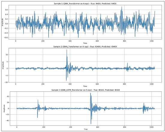
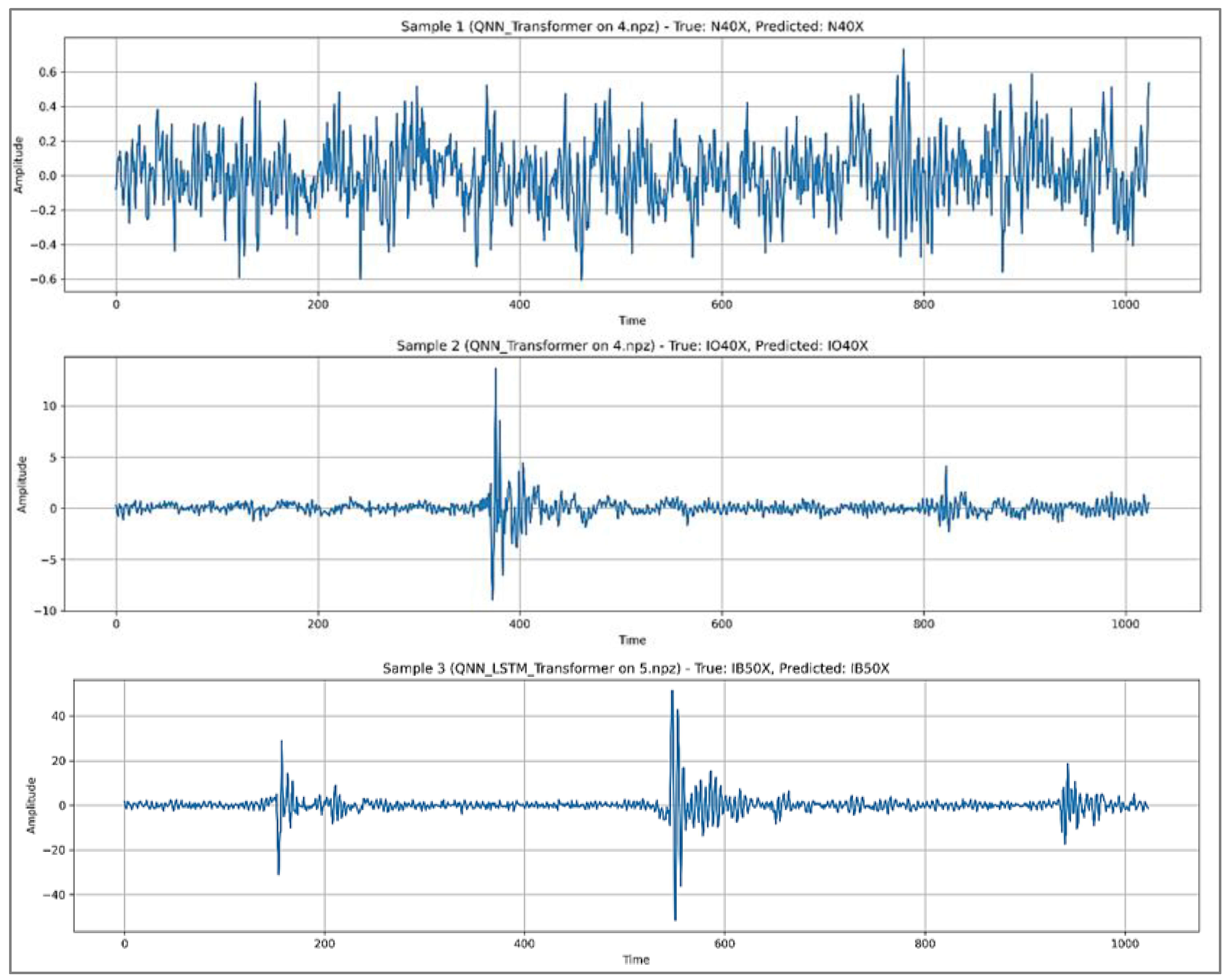
The architecture achieves perfect classification accuracy across three distinct datasets. This consistent performance validates the combinatorial hypothesis that heterogeneous but complementary technologies yield superior diagnostic capabilities with enhanced generalizability. Figure 6 shows the samples of the vibration signals tested true for bearing, outer and inner race faults along with normal signal of HUST data. Results are shown in Table 5. The proposed architecture achieves superior performance when subjected to varying operational conditions of industrial machines.

Figure 6. HUST data’s sample signals predicted by QuNN_LSTM_Transformer model.

Table 5. Summary of HUST dataset results.

HUST Dataset	4		5		6		7
Model Accuracy	Val	Test	Val	Test	Val	Test	Val	Test
CNN + LSTM	100	99.88	100	100	100	99.88	100	99.88
CNN + BiLSTM	100	99.88	100	100	100	100	100	99.88
CNN + Transformer	100	99.88	100	100	100	100	100	99.88
QNN + LSTM	100	99.88	100	100	100	100	100	99.88
QNN + BiLSTM	100	99.88	100	99.88	100	99.76	99.88	99.88
QNN + Transformer	100	100	100	100	100	100	100	100
QNN + LSTM + Transformer	100	100	100	100	100	100	100	100

Val—Validation.

4.4. Mendeley Data Results

Table 6 presents a detailed comparative analysis of hybrid deep learning models, assessing validation and test accuracies across the HSCP, HSOCD, VSCP, and VSOCD datasets. A clear observation is the consistent superiority of Quantum-inspired Neural Network (QuCNN)-based models over their classical Convolutional Neural Network (CNN) counterparts. On the HSCP dataset, the QuCNN-BiLSTM model achieves a 98.79% test accuracy, significantly outperforming the CNN_BiLSTM’s 97.28%.

Table 6. Summary of Mendeley dataset results.

Mendeley Dataset	HSCP		HSOCD		VSCP		VSOCD
Model Accuracy	Val	Test	Val	Test	Val	Test	Val	Test
CNN + LSTM	94.59	94.49	98.23	98.09	95.75	95.65	98.67	98.75
CNN + BiLSTM	97.38	97.28	98.85	98.72	99.52	99.51	99.60	99.59
CNN + Transformer	96.76	96.67	98.60	98.56	99.19	99.17	99.44	99.47
QuNN + LSTM	98.54	98.32	99.64	99.59	99.39	99.31	99.70	99.72
QuNN + BiLSTM	98.94	98.79	99.70	99.71	99.57	99.53	99.80	99.78
QuNN + Transformer	98.54	98.79	99.50	99.51	99.60	99.58	99.70	99.79
QNN-LSTM-Transformer	98.99	98.99	99.80	99.71	99.77	99.63	99.80	99.88

Val—Validation.

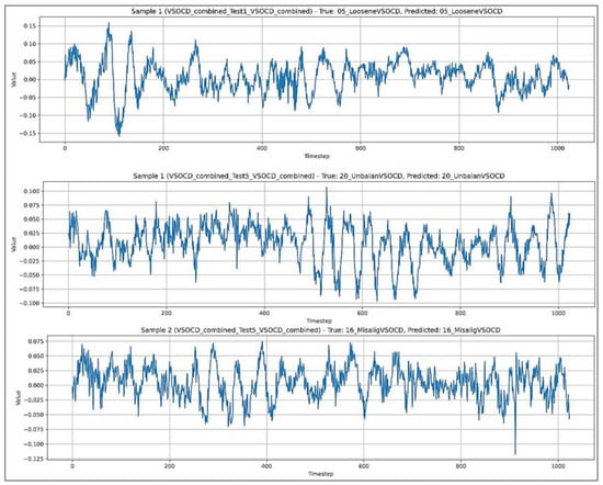
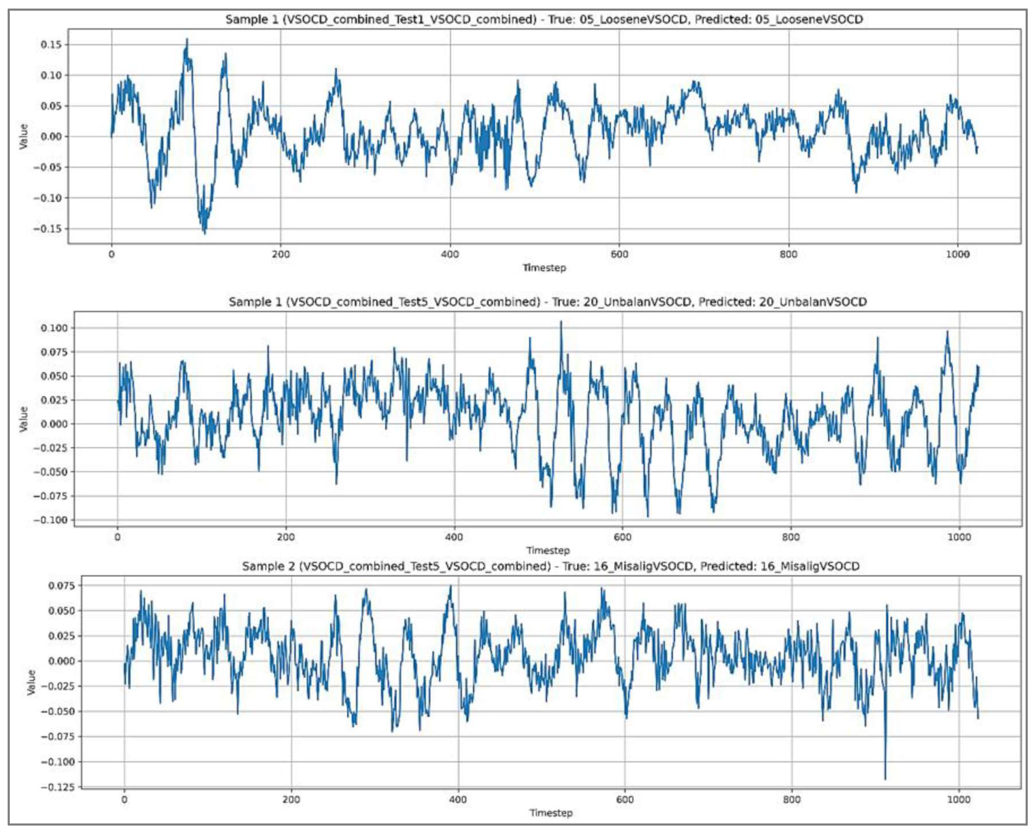
The integration of a Bidirectional LSTM (BiLSTM) provides a marked advantage over a standard LSTM, visible within both CNN and QUCNN frameworks. This enhancement is particularly significant when comparing the CNN-LSTM’s 95.65% test accuracy on VSCP to the CNN_BiLSTM’s 99.51%. While the Transformer architecture enhances performance in all combinations, the BiLSTM pairing often proves slightly more effective in these specific tests. All models demonstrate excellent generalization, with minimal deviation between validation and test accuracies across the board. The QUCNN-based models consistently achieve exceptional results, frequently exceeding 99.5% accuracy on the HSOCD, VSCP, and VSOCD datasets. Specifically, the QUCNN-BiLSTM model showcases outstanding performance, reaching 99.71% on HSOCD and 99.78% on VSOCD test sets. The combination of QUCNN with both LSTM and Transformer components proves to be a particularly potent architecture. This hybrid QUCNN-LSTM-Transformer model represents the pinnacle of performance in this evaluation. It secures top-tier accuracies across multiple datasets, culminating in the highest recorded score of 99.88% on the VSOCD test set. In conclusion, the results strongly affirm that hybridizing QUCNNs with advanced sequential models like BiLSTM and Transformer yields a state-of-the-art advantage, establishing a new performance benchmark for these tasks. Figure 7 shows the samples of the vibration signals tested true for looseness, unbalance and misalignment faults along with normal signal of Mendeley data.

Figure 7. Mendeley mechanical fault data’s sample signals predicted by QuNN_BiLSTM model.

4.5. Results Comparison

In the literature, several preprocessing steps have been applied to extract features from the data. The classification algorithms are applied on the features. Table 7 shows the proposed models’ performance to existing methods on three different datasets. The proposed model achieves an accuracy of 98.9% on all varying condition cases of the CWRU dataset, slightly lower than the existing methods. However, on individual fault diameters, it achieved at least higher than 99.4%. On HUST and the Mendeley mechanical faults dataset, the model achieved superior performance, maintaining its precise stability for reliable solution for industrial fault diagnosis. The proposed methodology maintains its performance when applied to complex hybrid industrial datasets.

Table 7. Results comparison with existing approaches.

Authors	Dataset	Model	Accuracy
[20]	CWRU	CNN	94.40
[21]		CNN_LSTM	94.46
[22]		CNN_LSTM	99.83
[23]		SWDCNN-RF	99.6
[24]		CRNN	99.7
[25]		CNN_LSTM	95
Proposed		QNN-LSTM-Transformer	98.9
[26]	HUST	CNN-LSTM	97.63
Proposed		QNN-LSTM-Transformer	100
[45]	Mendeley	CNN-GRU	96.79
[46]		U-Net	89%
[47]		Wavelet-Correlation	95%
Proposed		QNN-LSTM-Transformer	99.58

4.6. Misclassification and Error Analysis

The proposed architecture maintains consistent accuracy on the CWRU dataset, but an error rate of 1.06% occurs between ball bearing fault and outer race faults due to slight amplitude changes, which does not compromise a failure. A 100% safety recall measure for normal state indicates the requirements for industrial maintenance even under varying fault severities, as depicted in Table 8.

Table 8. Error analysis for CWRU dataset.

CWRU	7 Mils		14 Mils		21 Mils		All
Model Accuracy	Prec	Rec	Prec	Rec	Prec	Rec	Prec	Rec
Normal	100	100	100	100	100	100	100	100
Ball Fault	100	100	99.69	98.49	99.90	99.86	97.93	97.38
Inner Race	100	100	99.9	100	100	100	100	100
Outer Race	100	100	99.10	99.79	100	99.86	99.83	98.40

The proposed architecture shows 100% accuracy on the HUST dataset, showing excellent feature separability. However, the diagnostic conditions may not always be incorporated in a practical industrial environment. The physical properties of fault signatures would degrade the algorithmic performance due to material inconsistencies and high amplitudes during the processing. Material-induced misclassifications are to be isolated, ensuring no false alarms during the prediction.

The proposed architecture achieves nearly perfect diagnostic accuracy under different fault conditions for the Mendeley dataset, as shown in Table 9; there is a 0.13% to 3% error for a normal state to fault conditions like misalignment and unbalance, as there is a baseline vibration difference. This highly sensitive change is caused by sensor placement, and the algorithm can be misclassifying these transitional states of faults.

Table 9. Error analysis for Mendeley dataset.

Mendeley	HSCP		HSOCD		VSCP		VSOCD
Model Accuracy	Prec	Rec	Prec	Rec	Prec	Rec	Prec	Rec
Normal	98	97.02	99.6	99.6	100	100	99.87	99.87
Unbalance	100	100	99.90	99.84	99.10	99.07	100	100
Looseness	100	100	99.75	99.90	100	100	100	100
Misalignment	97.9	98.94	99.27	99.54	99.47	99.47	99.66	99.66

4.7. Ablation Study

A comprehensive ablation study is conducted to show the proposed model architecture and its analysis of each layer importance proving the necessity. Table 10 shows the performance in average accuracies of each model on three datasets on varying architecture configuration. The standard convolution layers when replaced with Quadratic neurons yielded a significant performance increase in two datasets. The non-linear interactions of amplitude fault frequencies were successfully extracted in the case of a huge dataset apt for real-time industrial environment. The LSTM layer tracking temporal patterns combined with transformers attention mechanism achieved nearly 99.5% accuracy across the three datasets.

Table 10. Ablation study performance results.

Model	Configuration	CWRU	HUST	Mendeley
Conv	With LSTM	99.40	99.94	96.745
Conv	With Transformer	99.59	99.94	98.692
Quadratic	With LSTM	98.97	99.94	99.235
Quadratic	With Transformer	98.92	100	99.4
Quadratic	With LSTM and Transformer	99.59	100	99.55

4.8. Computational Complexity

All models were evaluated using a batch size of 32 and signal sample of 1024 segments, as it captures full rotational cycle capturing fault impacts and to maintain computational efficiency. The no. of parameters utilized in CNN-LSTM are 215,236 parameters, approximately 0.21 million parameters, and QNN-LSTM-Transformer model utilizes 0.249 million parameters. While there is an increase in the no. of parameters, the proposed model is lightweight. The computational cost increases to 68.54 MFLOPs, with an algorithmic complexity of O(N2) over 256-step temporal sequence. Table 11 gives the computational complexity of the baseline model and the proposed model. The inference times are based on the computer speed with core GPU, scaled on 32 batch size.

Table 11. Computational complexity parameters.

Model	Parameters (M)	Computational Cost (MFLOPs)	Inference Time (ms/Segment)
CNN-LSTM	0.215	15.24	0.31
QNN-LSTM	0.212	44.80	0.58
QNN-LSTM-Transformer	0.249	68.54	0.85

4.9. Limitations and Future Work

While the proposed architecture demonstrates exceptional feature fault signatures tested on varying operational conditions of three datasets, the current study is limited by the absence of analysis under noise degradation. The background noise in industrial environments is frequent, and it might affect the early-stage defect signatures. Therefore, our future work will focus on a Signal-Noise-Ration sensitivity analysis. The architecture will be subjected to varying levels of noise conditions from favorable to severe noise (+10 dB to −10 dB) environments. The future work will also be validated against continuous empirical data acquired directly from active industrial environments by integrating Explainable Artificial Intelligence (XAI) techniques. The practical utility of Industrial Internet of Things computing node will be developed for predictive maintenance.

5. Conclusions

This comprehensive performance analysis establishes a new paradigm for hybrid deep learning approaches in vibration-based fault classification. Through systematic evaluation across heterogeneous datasets, the proposed methodologies demonstrate exceptional accuracy and reliability, validating their applicability under diverse operational conditions and complex fault signatures. The architectural progression from CNN-LSTM to QuCNN-LSTM-Transformer demonstrates clear performance enhancement for diagnostic accuracy, with all architectures exceeding 96% accuracy thresholds. The CNN versus QuCNN architecture comparison demonstrates a consistent advantage, where QUCNN architectures average 98.11% on the Mendeley data compared to 96.15% for CNN approaches, representing a significant 1.96% improvement. Overall, the QuCNN-LSTM-Transformer architecture emerges as the optimal solution for comprehensive fault classification, while the complete architectural spectrum provides flexibility for deployment across diverse operational requirements and computational constraints. This work offers a strategic framework in selecting an optimal architecture to various operational requirements of variable industrial datasets and performance objectives of vibration-based fault classification.

References

- Xu, M.; David, J.M.; Kim, S.H. The fourth industrial revolution: Opportunities and challenges. Int. J. Financ. Res. 2018, 9, 90–95. [Google Scholar] [CrossRef] [Scilit]
- Javaid, M.; Haleem, A.; Singh, R.P.; Suman, R. Artificial intelligence applications for industry 4.0: A literature-based study. J. Ind. Integr. Manag. 2022, 7, 83–111. [Google Scholar] [CrossRef] [Scilit]
- Akinbolajo, O. Predicting Equipment Failures Using Artificial Intelligence: A Proactive Approach. Int. J. Adv. Eng. Manag. 2025, 7, 513–521. [Google Scholar] [CrossRef] [Scilit]
- Gangsar, P.; Tiwari, R. Signal based condition monitoring techniques for fault detection and diagnosis of induction motors: A state-of-the-art review. Mech. Syst. Signal Process. 2020, 144, 106908. [Google Scholar] [CrossRef] [Scilit]
- Chemseddine, R.; Boualem, M.; Djamel, B.; Semchedine, F. Gear fault feature extraction and classification of singular value decomposition based on Hilbert empirical wavelet transform. J. Vibroeng. 2018, 20, 1603–1618. [Google Scholar] [CrossRef] [Scilit]
- Cerrada, M.; Zurita, G.; Cabrera, D.; Sánchez, R.V.; Artés, M.; Li, C. Fault diagnosis in spur gears based on genetic algorithm and random forest. Mech. Syst. Signal Process. 2016, 70–71, 87–103. [Google Scholar] [CrossRef] [Scilit]
- Dhakar, A.; Singh, B.; Gupta, P. Diagnosing faults in rolling bearings of an air compressor set up using local mean decomposition and support vector machine algorithm. J. Vib. Eng. Technol. 2024, 12, 6635–6648. [Google Scholar] [CrossRef] [Scilit]
- Li, X.; Wang, Y.; Yao, J.; Li, M.; Gao, Z. Multi-sensor fusion fault diagnosis method of wind turbine bearing based on adaptive convergent viewable neural networks. Reliab. Eng. Syst. Saf. 2024, 245, 109980. [Google Scholar] [CrossRef] [Scilit]
- Lee, C.Y.; Maceren, E.D. Induction motor bearing fault classification using deep neural network with particle swarm optimization-extreme gradient boosting. IET Electr. Power Appl. 2024, 18, 297–311. [Google Scholar]
- Zhang, L.; Lin, J.; Liu, B.; Zhang, Z.; Yan, X.; Wei, M. A review on deep learning applications in prognostics and health management. IEEE Access 2019, 7, 162415–162438. [Google Scholar] [CrossRef] [Scilit]
- Glowacz, A.; Sulowicz, M.; Kozik, J.; Piech, K.; Glowacz, W.; Li, Z.; Brumercik, F.; Gutten, M.; Korenciak, D.; Kumar, A.; et al. Fault diagnosis of electrical faults of three-phase induction motors using acoustic analysis. Bull. Pol. Acad. Sci. Tech. Sci. 2024, 72, e148440. [Google Scholar]
- Randall, R.B. State of the art in monitoring rotating machinery—Part 1. Sound Vib. 2004, 38, 14–21. [Google Scholar]
- Randall, R.B. Vibration-Based Condition Monitoring: Industrial, Automotive and Aerospace Applications; John Wiley & Sons: Hoboken, NJ, USA, 2021. [Google Scholar]
- Łuczak, D. Machine fault diagnosis through vibration analysis: Continuous wavelet transforms with complex morlet wavelet and time–frequency RGB image recognition via convolutional neural network. Electronics 2024, 13, 452. [Google Scholar] [CrossRef] [Scilit]
- Xu, M.; Gao, J.; Zhang, Z.; Wang, H. Bearing-fault diagnosis with signal-to-rgb image mapping and multichannel multiscale convolutional neural network. Entropy 2022, 24, 1569. [Google Scholar] [CrossRef] [Scilit]
- Yang, W.; Wu, Z.; Ma, L.; Guo, L.; Chang, Y. EffiMultiOrthoBearNet: An Efficient Lightweight Architecture for Bearing Fault Diagnosis. Electronics 2024, 13, 3081. [Google Scholar]
- Saeed, A.; Akram, M.U.; Khattak, M.; Khan, M.B. An interpretable hybrid framework combining convolution latent vectors with transformer-based attention mechanism for rolling element fault detection and classification. Heliyon 2024, 10, e38993. [Google Scholar]
- Fan, Y.; Fu, Z.; Li, H.; Yang, Y. Motor bearing fault diagnosis based on LMSWT with improved multi-scale convolutional neural network. IEEE Trans. Instrum. Meas. 2025, 74, 3537011. [Google Scholar]
- Chennana, A.; Megherbi, A.C.; Bessous, N.; Sbaa, S.; Teta, A.; Belabbaci, E.O.; Rabehi, A.; Guermoui, M.; Agajie, T.F. Vibration signal analysis for rolling bearings faults diagnosis based on deep-shallow features fusion. Sci. Rep. 2025, 15, 9270. [Google Scholar] [CrossRef] [Scilit]
- Ding, X.; Wang, H.; Cao, Z.; Liu, X.; Liu, Y.; Huang, Z. An edge intelligent method for bearing fault diagnosis based on a parameter transplantation convolutional neural network. Electronics 2023, 12, 1816. [Google Scholar] [CrossRef] [Scilit]
- Masih, B. Classification of Bearing Failure in Adverse Industrial Conditions. Master’s Thesis, Chulalongkorn University, Bangkok, Thailand, 2024. Available online: https://digital.car.chula.ac.th/chulaetd/12232 (accessed on 1 July 2023).
- Wei, L.; Peng, X.; Cao, Y. Enhanced fault diagnosis of rolling bearings using an improved inception-lstm network. Nondestruct. Test. Eval. 2025, 40, 3274–3293. [Google Scholar] [CrossRef] [Scilit]
- Zhang, Q.; Yao, Y.; Huang, Y.; Liu, Y.; Wu, L. A Bearing Fault Diagnosis Model Based on a Simplified Wide Convolutional Neural Network and Random Forrest. Sensors 2025, 25, 752. [Google Scholar] [CrossRef] [Scilit] [PubMed]
- Khorram, A.; Khalooei, M.; Rezghi, M. End-to-end CNN+ LSTM deep learning approach for bearing fault diagnosis: End-to-End CNN+ LSTM Deep Learning Approach for Bearing Fault Diagnosis. Appl. Intell. 2021, 51, 736–751. [Google Scholar] [CrossRef] [Scilit]
- Sun, H.; Fan, Y. Fault diagnosis of rolling bearings based on CNN and LSTM networks under mixed load and noise. Multimed. Tools Appl. 2023, 82, 43543–43567. [Google Scholar] [CrossRef] [Scilit]
- Abbasi, M.A.; Huang, S.; Khan, A.S. Fault detection and classification of motor bearings under multiple operating conditions. ISA Trans. 2025, 156, 61–69. [Google Scholar] [CrossRef] [Scilit]
- Smith, W.A.; Randall, R.B. Rolling element bearing diagnostics using the Case Western Reserve University data: A benchmark study. Mech. Syst. Signal Process. 2015, 64–65, 100–131. [Google Scholar] [CrossRef] [Scilit]
- Case School of Engineering. Available online: https://engineering.case.edu/bearingdatacenter/welcome (accessed on 1 July 2023).
- Thuan, N.D.; Hong, H.S. HUST Bearing: A Practical Dataset for Ball Bearing Fault Diagnosis. BMC Res. Notes 2023, 16, 138. [Google Scholar] [CrossRef] [Scilit]
- HUST Bearing Dataset. Available online: https://data.mendeley.com/datasets/cbv7jyx4p9/1 (accessed on 1 July 2023).
- Brito, L.C.; Susto, G.A.; Brito, J.N.; Duarte, M.A. Mechanical Faults in Rotating Machinery Dataset (Normal, Unbalance, Misalignment, Looseness). Available online: https://data.mendeley.com/datasets/zx8pfhdtnb/3 (accessed on 1 July 2023).
- Ng, K.W.; Huang, Y.F.; Koo, C.H.; Chong, K.L.; El-Shafie, A.; Ahmed, A.N. A review of hybrid deep learning applications for streamflow forecasting. J. Hydrol. 2023, 625, 130141. [Google Scholar] [CrossRef] [Scilit]
- Fan, Y.; Tang, Q.; Guo, Y.; Wei, Y. BiLSTM-MLAM: A multi-scale time series prediction model for sensor data based on Bi-LSTM and local attention mechanisms. Sensors 2024, 24, 3962. [Google Scholar] [CrossRef] [Scilit]
- Hajigholam Saryazdi, A. A Novel Hybrid Deep Learning Model for Electricity Price Forecasting. SSRN 2024, 5166713. [Google Scholar] [CrossRef] [Scilit]
- Vaswani, A.; Shazeer, N.; Parmar, N.; Uszkoreit, J.; Jones, L.; Gomez, A.N.; Kaiser, Ł.; Polosukhin, I. Attention is all you need. In Proceedings of the 31st International Conference on Neural Information Processing Systems, Long Beach, CA, USA, 4–9 December 2017; Volume 30. [Google Scholar]
- Wen, Q.; Zhou, T.; Zhang, C.; Chen, W.; Ma, Z.; Yan, J.; Sun, L. Transformers in time series: A survey. arXiv 2022, arXiv:2202.07125. [Google Scholar]
- Saraswat, M.; Dubey, A.K. EBi-LSTM: An enhanced bi-directional LSTM for time-series data classification by heuristic development of optimal feature integration in brain computer interface. Comput. Methods Biomech. Biomed. Eng. 2024, 27, 378–399. [Google Scholar] [CrossRef] [Scilit] [PubMed]
- Arbane, M.; Benlamri, R.; Brik, Y.; Alahmar, A.D. social media-based COVID-19 sentiment classification model using Bi-LSTM. Expert Syst. Appl. 2023, 212, 118710. [Google Scholar] [CrossRef] [Scilit] [PubMed]
- Adefemi, K.O.; Mutanga, M.B. A robust hybrid CNN–LSTM model for predicting student academic performance. Digital 2025, 5, 16. [Google Scholar] [CrossRef] [Scilit]
- Hassan, N.; Miah, A.S.; Shin, J. A deep bidirectional LSTM model enhanced by transfer-learning-based feature extraction for dynamic human activity recognition. Appl. Sci. 2024, 14, 603. [Google Scholar] [CrossRef] [Scilit]
- Song, K.Y.; Tiong, L.C.; Lee, Y. See through the noise: Revolutionizing medical image diagnosis with quadratic convolutional neural network (Q-CNN). Int. J. Mach. Learn. Cybern. 2025, 16, 2615–2633. [Google Scholar] [CrossRef] [Scilit]
- Kim, T.; Vecchietti, L.F.; Choi, K.; Lee, S.; Har, D. Machine learning for advanced wireless sensor networks: A review. IEEE Sens. J. 2020, 21, 12379–12397. [Google Scholar] [CrossRef] [Scilit]
- Peng, H.; Yang, J.; Wang, J.; Wang, T.; Sun, Z.; Song, X.; Luo, X.; Huang, X. Spiking neural P systems with multiple channels. Neural Netw. 2017, 95, 66–71. [Google Scholar] [CrossRef] [Scilit]
- Sarao Mannelli, S.; Vanden-Eijnden, E.; Zdeborová, L. Optimization and generalization of shallow neural networks with quadratic activation functions. In Proceedings of the 34th International Conference on Neural Information Processing Systems, Vancouver, BC, Canada, 6–12 December 2020; Volume 33, pp. 13445–13455. [Google Scholar]
- Zhang, W.; Meng, H.; Wang, R.; Wang, P. Intelligent optimized diagnosis for hydropower units based on CEEMDAN combined with RCMFDE and ISMA-CNN-GRU-attention. Water 2025, 17, 2125. [Google Scholar] [CrossRef] [Scilit]
- Jeong, H.; Kim, S.; Seo, D.; Kwon, J. Source-free domain adaptation framework for rotary machine fault diagnosis. Sensors 2025, 25, 4383. [Google Scholar] [CrossRef] [Scilit]
- Rezazadeh, N.; De Oliveira, M.; Lamanna, G.; Perfetto, D.; De Luca, A. WaveCORAL-DCCA: A Scalable Solution for Rotor Fault Diagnosis Across Operational Variabilities. Electronics 2025, 14, 3146. [Google Scholar] [CrossRef] [Scilit]
Disclaimer/Publisher’s Note: The statements, opinions and data contained in all publications are solely those of the individual author(s) and contributor(s) and not of MDPI and/or the editor(s). MDPI and/or the editor(s) disclaim responsibility for any injury to people or property resulting from any ideas, methods, instructions or products referred to in the content. |
© 2026 by the authors. Licensee MDPI, Basel, Switzerland. This article is an open access article distributed under the terms and conditions of the Creative Commons Attribution (CC BY) license.