Robust Backstepping Control of a Twin Rotor MIMO System via an RBF-Tuned High-Gain Observer

Abstract

The design of robust controllers for complex nonlinear systems remains a formidable challenge, particularly concerning the disparity between simulation performance and real-world implementation constraints. This research investigates the practical implementation of a backstepping controller integrated with a High-Gain Observer (HGO) on a Twin Rotor MIMO System (TRMS). While the control architecture exhibited stability and precise tracking in simulation, physical deployment initially failed due to sensitivity to measurement noise and the peaking phenomenon, resulting in a divergent response with a Yaw RMSE of 2.56 rad. Unlike conventional approaches that attempt to bridge the simulation-to-reality gap by optimizing the controller, we hypothesized that the critical bottleneck lay within the observer dynamics. To address this, a Radial Basis Function (RBF) Neural Network was employed to adaptively tune the observer gains in real time. Experimental results demonstrate that this adaptive mechanism successfully mitigated the effects of unmodeled dynamics and noise, reducing the Root Mean Square Error (RMSE) by over 85% in the pitch axis and 95% in the yaw axis. These findings substantiate that online adaptive observer tuning is a decisive strategy for ensuring the reliability of advanced nonlinear controllers on physical hardware.

1. Introduction

The rapid evolution of modern aerospace and robotics, particularly within the unmanned aerial vehicle (UAV) sector, has imposed increasingly stringent requirements on flight control systems. These platforms are characterized by significant challenges, including high cross-coupling between axes, inherent nonlinearities, and underactuated dynamics, making precise and robust control a formidable task. To validate new control strategies before deployment, researchers frequently utilize laboratory-scale benchmark systems that accurately emulate these complex dynamics. Among these, the Twin Rotor Multiple-Input Multiple-Output (TRMS) system is one of the most widely recognized testing platforms [1]. By simulating the fundamental behavior of a helicopter, the TRMS provides a robust environment for evaluating sophisticated flight control and optimization schemes.

Initial research into TRMS control focused largely on classical and optimal control theories. Proportional–Integral–Derivative (PID) controllers are frequently employed due to their simplicity and reliability in localized operating regions. Additionally, optimal control methods such as the Linear Quadratic Integral (LQI) and Linear Quadratic Gaussian (LQG) controllers have been proposed to meet specific performance objectives while minimizing cost functions [2]. However, because these methods rely on linearized models, their effectiveness often diminishes when the system operates across a wide range or encounters significant nonlinearities.

To address these limitations, the community has shifted toward advanced nonlinear control schemes. Robust techniques, such as Sliding Mode Control (SMC) [3] and Feedback Linearization [4], have been applied to the TRMS to directly manage system nonlinearities. Backstepping control, in particular, has emerged as a powerful recursive design methodology that ensures stability through the strategic selection of Lyapunov functions [5]. Developed originally by Krstic et al. [6], backstepping is uniquely suited for systems in strict-feedback form, allowing for the recursive stabilization of subsystems until a final control law is derived. This approach has been successfully implemented in various domains, including trajectory tracking for mobile robots [7] and motor control [8]. Recent studies have further enhanced backstepping by integrating it with Sliding Mode Control [9] or disturbance observers [10] to handle increased complexity.

Because backstepping requires full-state feedback, an observer is necessary when only outputs are measurable. The High-Gain Observer (HGO) is a popular choice for nonlinear systems due to its rapid convergence properties [11]. However, physical implementation of a standard HGO is often hindered by the peaking phenomenon and extreme sensitivity to measurement noise [11]. To mitigate these issues, advanced structures such as filtered HGOs or multi-observer designs have been developed [12,13,14,15,16]. Despite the theoretical success of combined backstepping and HGO architectures, a significant “simulation-to-real-time” gap often exists due to discrepancies between idealized models and physical hardware [17].

To bridge this gap, this paper proposes a novel adaptive control structure that integrates a Radial Basis Function (RBF) Neural Network with a backstepping controller and an HGO. While previous work explored Type-2 Takagi-Sugeno fuzzy logic for this purpose [18], the transition to hardware requires even faster adaptation. RBF networks are utilized here as universal approximators to counteract unmodeled dynamics that are difficult to characterize analytically [19,20,21,22,23]. The core contribution of this work is the real-time, online tuning of HGO parameters using an RBF network to overcome the implementation bottlenecks of the TRMS. The remainder of this paper is structured as follows: Section 2 details the methodology, including the TRMS model and the design of the adaptive controller; Section 3 presents simulation and experimental results; and Section 4 concludes the study.

2. Materials and Methods

2.1. Plant Model

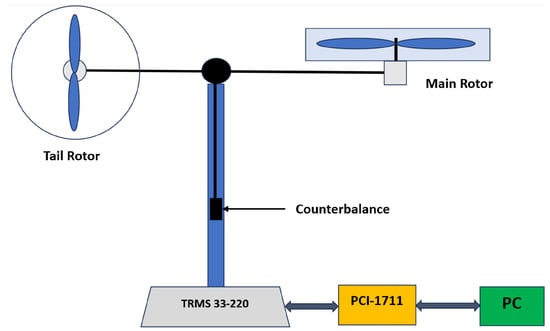
The Twin Rotor Multi-Input Multi-Output System (TRMS), manufactured by Feedback Instruments Ltd. (Crowborough, UK), is a laboratory device which simulates the behavior of a helicopter, as indicated in the manual provided by the manufacturer [22]. The equipment consists of a horizontal beam pivoted on a vertical tower, with the ends of the beam capped by two propellers: a main rotor and a tail rotor. To provide overall static stability, a counterweight is added. This design allows the beam to rotate freely, performing pitch and yaw movements, making the system an appropriate reference point for investigating complex multivariable control problems. The control unit located at the base of the apparatus includes an input/output (I/O) subsystem connecting a computer to a sensor data stream as real-time data, acting as an interface to implement the closed-loop controller. The general form of the nonlinear state space model can be used to describe the dynamics of the system, and the physical architecture of the apparatus is illustrated in Figure 1:

$$\left\{\begin{array}{c}\dot{x}=f(x,u,t)\hfill \\ y=g(x,u,t)\hfill \end{array}\right.$$

(1)

where: $x\in R^n$ is the state vector, $u\in R^m$ is the control input vector, and $y\in R^p$ is the output vector.

Figure 1. Schematic diagram of the Twin Rotor MIMO System (TRMS) illustrating the main rotor, tail rotor, and degrees of freedom.

Following the validated methodology in [24,25], the specific nonlinear model for the TRMS used in this work is described by a set of six first-order differential equations. The state vector is defined as $x={[x_1,x_2,x_3,x_4,x_5,x_6]}^T={[\psi ,\dot{\psi },\varphi ,\dot{\varphi },{\tau }_1,{\tau }_2]}^T$, where $\psi$ is the pitch angle, $\varphi$ is the yaw angle, and ${\tau }_1$ and ${\tau }_2$ are the torques generated by the main and tail rotors, respectively. The control inputs are the voltages applied to the main and tail motors $u={[U_1,U_2]}^T$. The system dynamics are given by:

$$\left\{\begin{array}{c}{\dot{x}}_1=x_2\hfill \\ {\dot{x}}_2={\displaystyle \frac{1}{I_1}}(a_1{x}_5^2+b_1{x}_5-M_{g}sin{x}_1-B_{1\psi }{x}_2-B_{2\psi }\mathrm{sgn}\left(x_2\right)-K_{gy}{x}_{4}cos\left(x_1\right)(a_1{x}_5^2+b_1{x}_5))\hfill \\ {\dot{x}}_3=x_4\hfill \\ {\dot{x}}_4={\displaystyle \frac{1}{I_2}}(a_2{x}_6^2+b_2{x}_6-B_{1\varphi }{x}_4-B_{2\varphi }\mathrm{sgn}\left(x_4\right)-1.75K_c(a_1{x}_5^2+b_1{x}_5))\hfill \\ {\dot{x}}_5=-{\displaystyle \frac{T_{10}}{T_{11}}}{x}_5+{\displaystyle \frac{K_1}{T_{11}}}{U}_1\hfill \\ {\dot{x}}_6=-{\displaystyle \frac{T_{20}}{T_{21}}}{x}_6+{\displaystyle \frac{K_2}{T_{21}}}{U}_2\hfill \end{array}\right.$$

(2)

The system output vector consists of the directly measurable pitch and yaw angles:

$$y={[x_1,x_3]}^T={[\psi ,\varphi ]}^T$$

(3)

The parameters in Equation (2) represent the physical properties of the system, including moments of inertia ($I_1,I_2$), aerodynamic force and torque constants ($a_1,b_1,a_2,b_2$), gravitational moments ($M_g$), friction coefficients ($B_{1\psi },B_{2\psi },B_{1\varphi },B_{2\varphi }$), gyroscopic cross-coupling gains ($K_{gy},K_c$), and motor dynamics parameters ($T_{10},T_{11},K_1,T_{20},T_{21},K_2$). The specific numerical values for all these parameters are detailed in the manufacturer’s manual [26].

2.2. Backstepping Control

Backstepping is a recognised tool for the design of controllers for nonlinear systems [5,6]. However, the state model given in (2) does not fit the strict-feedback structure, thus creating a mismatch with the standard requisites for backstepping. The way around this is to use a decentralised approach where the dynamics of the pitch and the yaw are handled separately with the intercoupling seen as a disturbance to be rejected by the controller.

The systematic design for both subsystems is explained below:

2.2.1. Backstepping Control for the Pitch Subsystem

For the controller synthesis, the cross-coupling terms are omitted from the state equations and are treated as external disturbances. Thus, the design model differs slightly from the full plant model in (2). The decentralized model for the pitch subsystem is given by:

$$\left\{\begin{array}{c}{\dot{x}}_1=x_2\hfill \\ {\dot{x}}_2={\displaystyle \frac{1}{I_1}}(a_1{x}_3^2+b_1{x}_3-M_{g}sin{x}_1-B_{1\psi }{x}_2-B_{2\psi }\left(x_1\right))\hfill \\ {\dot{x}}_3=-{\displaystyle \frac{T_{10}}{T_{11}}}{x}_3+{\displaystyle \frac{K_1}{T_{11}}}{U}_1\hfill \end{array}\right.$$

(4)

where $x_1=\psi$, $x_2=\dot{\psi }$, $x_3={\tau }_1$, and $U_1$ is the control input. Note: The state indices are redefined locally for this subsystem; specifically, $x_3$ here corresponds to the main rotor torque $x_5$ in the full plant model (2). The backstepping design proceeds in three steps to ensure the state $x_1$ tracks a desired trajectory $x_{1d}$.

Step 1: Primary Tracking Error and First Virtual Control

The design begins by defining the tracking error for the pitch angle, $z_1$, as the difference between the actual state $x_1$ and the desired trajectory $x_{1d}$:

$$z_1=x_1-x_{1d}$$

(5)

To analyze the error dynamics, a candidate Lyapunov function $V_1={\displaystyle \frac{1}{2}}{z}_1^2$ is selected. Its time derivative is found by using the derivative of the error, ${\dot{z}}_1=x_2-{\dot{x}}_{1d}$ as follows:

$${\dot{V}}_1=z_1{\dot{z}}_1=z_1(x_2-{\dot{x}}_{1d})$$

(6)

In this expression, the state $x_2$ acts as a control input for the $z_1$ subsystem. It is therefore treated as a virtual control, and a stabilizing function, ${\alpha }_1$, is designed as follows:

$${\alpha }_1=-c_1{z}_1+{\dot{x}}_{1d}$$

(7)

where $c_1>0$ is a positive design constant. The discrepancy between the state $x_2$ and its stabilizing function ${\alpha }_1$ is defined as a new error variable, $z_2$ given by:

$$z_2=x_2-{\alpha }_1$$

(8)

Substituting this into the derivative of $V_1$ yields:

$${\dot{V}}_1=-c_1{z}_1^2+z_1{z}_2$$

(9)

The term $-c_1{z}_1^2$ is stabilizing, but the indefinite cross-term $z_1{z}_2$ must be addressed in the subsequent step.

Step 2: Stabilization of the Augmented Pitch Subsystem

The second step addresses the stabilization of the $z_2$ error. The dynamics of this error, ${\dot{z}}_2={\dot{x}}_2-{\dot{\alpha }}_1$, must first be evaluated. The dynamic of ${\dot{x}}_2$ is:

$${\dot{x}}_2={\displaystyle \frac{1}{I_1}}(a_1{x}_2^2+b_1{x}_3-M_{g}sin{x}_1-B_{1\psi }{x}_2-B_{2\psi }\left(x_1\right))$$

(10)

The time derivative of the virtual control ${\alpha }_1$ is:

$${\dot{\alpha }}_1={\displaystyle \frac{\partial {\alpha }_1}{\partial z_1}}{\dot{z}}_1+{\displaystyle \frac{\partial {\alpha }_1}{\partial {\dot{x}}_{1d}}}{\ddot{x}}_{1d}=-c_1(x_2-{\dot{x}}_{1d})+{\ddot{x}}_{1d}$$

(11)

Substituting into the expression for ${\dot{z}}_2$ gives its complete form as:

$${\dot{z}}_2={\displaystyle \frac{1}{I_1}}(a_1{x}_2^2+b_1{x}_3-M_{g}sin{x}_1-B_{1\psi }{x}_2-B_{2\psi }\left(x_1\right))+c_1{x}_2-c_1{\dot{x}}_{1d}-{\ddot{x}}_{1d}$$

(12)

Now, the Lyapunov function is augmented to $V_2=V_1+{\displaystyle \frac{1}{2}}{z}_2^2$. Its time derivative is:

$${\dot{V}}_2=-c_1{z}_1^2+z_1{z}_2+z_2({\dot{x}}_2-{\dot{\alpha }}_1)$$

(13)

To continue the recursive design, the terms influenced by the true control input (via $x_3$) are grouped into a new variable, E:

$$E={\displaystyle \frac{1}{I_1}}(a_1{x}_2^2+b_1{x}_3-B_{1\psi }{x}_2)$$

(14)

Now, E is treated as the next virtual control. A second stabilizing function, ${\alpha }_2$, is designed for E, and a final error variable, $z_3=E-{\alpha }_2$, is introduced. The function ${\alpha }_2$ is strategically chosen to ensure stability:

$${\alpha }_2=-c_2{z}_2-z_1+{\displaystyle \frac{1}{I_1}}(M_{g}sin{x}_1+B_{2\psi }\left(x_1\right))-c_1{x}_2+c_1{\dot{x}}_{1d}+{\ddot{x}}_{1d}$$

(15)

where $c_2>0$. With this structure, the derivative of the Lyapunov function simplifies to:

$${\dot{V}}_2=-c_1{z}_1^2-c_2{z}_2^2+z_2{z}_3$$

(16)

Step 3: Derivation of the Final Pitch Control Law

The final step derives the actual control input $U_1$. The complete Lyapunov function for the system is

$$V_3=V_2+{\displaystyle \frac{1}{2}}{z}_3^2$$

(17)

Its time derivative is ${\dot{V}}_3={\dot{V}}_2+z_3{\dot{z}}_3$. The error dynamic ${\dot{z}}_3$ is first established below:

$${\dot{z}}_3=\dot{E}-{\dot{\alpha }}_2$$

(18)

The expression for $\dot{E}$ is found by differentiating (13), which requires the dynamic of ${\dot{x}}_3$ as follows:

$${\dot{x}}_3=-{\displaystyle \frac{T_{10}}{T_{11}}}{x}_3+{\displaystyle \frac{K_1}{T_{11}}}{U}_1$$

(19)

This leads to:

$$\dot{E}={\displaystyle \frac{1}{I_1}}[(2a_1{x}_3+b_1){\dot{x}}_3-B_{1\psi }{\dot{x}}_2]$$

(20)

Substituting (19) into (20) gives $\dot{E}$ as an explicit function of $U_1$:

$$\dot{E}={\displaystyle \frac{1}{I_1}}\left[(2a_1{x}_3+b_1)\left(-{\displaystyle \frac{T_{10}}{T_{11}}}{x}_3+{\displaystyle \frac{K_1}{T_{11}}}{U}_1\right)-B_{1\psi }{\dot{x}}_2\right]$$

(21)

The derivative of the second virtual control, ${\dot{\alpha }}_2$, is also required:

$${\dot{\alpha }}_2={\displaystyle \frac{M_{g}cos\left(x_1\right)}{I_1}}{x}_2-c_1{\dot{x}}_2-(x_2-{\dot{x}}_{1d})-c_2(z_3-z_1-c_2{z}_2)+c_1{\dot{x}}_{1d}+{\ddot{x}}_{1d}$$

(22)

Returning to the Lyapunov derivative, ${\dot{V}}_3$ can be written as:

$${\dot{V}}_3=-c_1{z}_1^2-c_2{z}_2^2+z_3(\dot{E}-{\dot{\alpha }}_2)$$

(23)

To render ${\dot{V}}_3$ negative definite, the control $U_1$ is chosen to enforce the following condition:

$$\begin{array}{c}\hfill {\displaystyle \frac{1}{I_1}}\left[(2a_1{x}_3+b_1)\left(-{\displaystyle \frac{T_{10}}{T_{11}}}{x}_3+{\displaystyle \frac{K_1}{T_{11}}}{U}_1\right)-B_{1\psi }{\dot{x}}_2\right]-[{\displaystyle \frac{M_{g}cos\left(x_1\right)}{I_1}}{x}_2-c_1{\dot{x}}_2-(x_2-{\dot{x}}_{1d})\\ \hfill -c_2(z_3-z_1-c_2{z}_2)+c_1{\dot{x}}_{1d}+{\ddot{x}}_{1d}]=-z_2-c_3{z}_3\end{array}$$

(24)

where $c_3>0$. By substituting the expanded forms of $\dot{E}$ (from (21)) and ${\dot{\alpha }}_2$ (from (22)) into (24) and isolating the $U_1$ term, we obtain the final control law:

$$\begin{array}{c}\hfill U_1=\left({\displaystyle \frac{T_{11}}{K_1(2a_1{x}_3+b_1)}}\right)(-z_2-c_3{z}_3+{\displaystyle \frac{M_{g}cos\left(x_1\right)}{I_1}}{x}_2-c_1{\dot{x}}_2-(x_2-{\dot{x}}_{1d})-c_2(z_3-z_1-c_2{z}_2)\\ \hfill +{\displaystyle \frac{T_{10}}{T_{11}}}{x}_3+{\displaystyle \frac{B_{1\psi }}{I_1}}{\dot{x}}_2+c_1{\dot{x}}_{1d}+{\ddot{x}}_{1d})\end{array}$$

(25)

This control law satisfies the design condition from Equation (24). As a result, it guarantees that the derivative of the Lyapunov function is always negative.

$${\dot{V}}_3=-c_1{z}_1^2-c_2{z}_2^2-c_3{z}_3^2<0,$$

(26)

This result formally proves that the pitch tracking error is globally asymptotically stable. We designed the controller for the yaw subsystem using an analogous three-step procedure.

2.2.2. Backstepping Control for the Yaw Subsystem

We designed the yaw controller using the same process as the pitch controller. It follows the same three-step method to make sure the yaw angle robustly follows its desired path, $x_{2d}$. The simplified model used for the yaw subsystem is shown in (27) as:

$$\left\{\begin{array}{c}{\dot{x}}_4=x_5\hfill \\ {\dot{x}}_5={\displaystyle \frac{1}{I_2}}(a_2{x}_6^2+b_2{x}_6-B_{1\varphi }{x}_5-B_{2\varphi }{x}_4)\hfill \\ {\dot{x}}_6=-{\displaystyle \frac{T_{20}}{T_{21}}}{x}_6+{\displaystyle \frac{K_2}{T_{21}}}{U}_2\hfill \end{array}\right.$$

(27)

where $x_4=\varphi$, $x_5=\dot{\varphi }$, $x_6={\tau }_2$, and $U_2$ is the control input.

Step 1: Tracking Error and First Virtual Control

The tracking error is defined as:

$$z_4=x_4-x_{2d}$$

(28)

The stability of this error is analyzed using the Lyapunov candidate $V_4={\displaystyle \frac{1}{2}}{z}_4^2$, whose time derivative is:

$${\dot{V}}_4=z_4{\dot{z}}_4=z_4(x_5-{\dot{x}}_{2d})$$

(29)

As before, the state $x_5$ is treated as a virtual control, and a stabilizing function ${\alpha }_4$ is designed for it:

$${\alpha }_4=-c_4{z}_4+{\dot{x}}_{2d}$$

(30)

where $c_4>0$. The discrepancy between the state $x_5$ and its virtual control ${\alpha }_4$ is defined as the new error variable, $z_5$:

$$z_5=x_5-{\alpha }_4$$

(31)

Substituting this into ${\dot{V}}_4$ yields:

$${\dot{V}}_4=-c_4{z}_4^2+z_4{z}_5$$

(32)

Step 2: Stabilization of the Augmented System

The second step focuses on stabilizing the $z_5$ error. The analysis requires the derivative ${\dot{z}}_5={\dot{x}}_5-{\dot{\alpha }}_4$, which in turn requires the dynamics of ${\dot{x}}_5$ and ${\dot{\alpha }}_4$:

$${\dot{x}}_5={\displaystyle \frac{1}{I_2}}(a_2{x}_6^2+b_2{x}_6-B_{1\varphi }{x}_5-B_{2\varphi }{x}_4)$$

(33)

$${\dot{\alpha }}_4=-c_4(x_5-{\dot{x}}_{2d})+{\ddot{x}}_{2d}$$

(34)

Substituting these into the ${\dot{z}}_5$ expression gives its full form:

$${\dot{z}}_5={\displaystyle \frac{1}{I_2}}(a_2{x}_6^2+b_2{x}_6-B_{1\varphi }{x}_5-B_{2\varphi }\left(x_4\right))+c_4{x}_5-c_4{\dot{x}}_{2d}-{\ddot{x}}_{2d}$$

(35)

The Lyapunov function is now augmented to $V_5=V_4+{\displaystyle \frac{1}{2}}{z}_5^2$. The term F is introduced to encapsulate the dynamics influenced by the true control input $U_2$ (via $x_6$):

$$F={\displaystyle \frac{1}{I_2}}(a_2{x}_6^2+b_2{x}_6-B_{1\varphi }{x}_5)$$

(36)

A final error variable $z_6=F-{\alpha }_5$ is defined, where ${\alpha }_5$ is the second virtual control, designed as:

$${\alpha }_5=-c_5{z}_5-z_4+{\displaystyle \frac{1}{I_2}}(B_{2\varphi }\left(x_4\right))-c_4{x}_5+c_4{\dot{x}}_{2d}+{\ddot{x}}_{2d}$$

(37)

With $c_5>0$. The term $-z_4$ is included to cancel the $z_4{z}_5$ term that will arise in the Lyapunov derivative. The ${\dot{z}}_5$ dynamic can now be expressed as:

$${\dot{z}}_5=z_6+{\alpha }_5-{\displaystyle \frac{1}{I_2}}(B_{2\varphi }\left(x_4\right))+c_4{x}_5-c_4{\dot{x}}_{2d}-{\ddot{x}}_{2d}$$

(38)

Using this structure, the derivative of the augmented Lyapunov function simplifies to:

$${\dot{V}}_5=-c_4{z}_4^2-c_5{z}_5^2+z_5{z}_6$$

(39)

Step 3: Derivation of the Final Control Law

The final step derives the actual control input $U_2$. The complete Lyapunov function is:

$$V_6=V_5+{\displaystyle \frac{1}{2}}{z}_6^2$$

(40)

Its time derivative is ${\dot{V}}_6={\dot{V}}_5+z_6{\dot{z}}_6$, where ${\dot{z}}_6=\dot{F}-{\dot{\alpha }}_5$. To solve this, the expressions for $\dot{F}$ and ${\dot{\alpha }}_5$ are required. $\dot{F}$ is found by differentiating Equation (36):

$$\dot{F}={\displaystyle \frac{1}{I_2}}\left[(2a_2{x}_6+b_2){\dot{x}}_6-B_{1\varphi }{\dot{x}}_5\right]$$

(41)

where the dynamic of ${\dot{x}}_6$ is given by:

$${\dot{x}}_6=-{\displaystyle \frac{T_{20}}{T_{21}}}{x}_6+{\displaystyle \frac{K_2}{T_{21}}}{U}_2$$

(42)

Substituting (42) into (41) gives $\dot{F}$ as an explicit function of $U_2$:

$$\dot{F}={\displaystyle \frac{1}{I_2}}\left[(2a_2{x}_6+b_2)\left(-{\displaystyle \frac{T_{20}}{T_{21}}}{x}_6+{\displaystyle \frac{K_2}{T_{21}}}{U}_2\right)-B_{1\varphi }{\dot{x}}_5\right]$$

(43)

The derivative of the second virtual control, ${\dot{\alpha }}_5$, is also computed:

$${\dot{\alpha }}_5=-c_4{\dot{x}}_5-(x_5-{\dot{x}}_{2d})-c_5(z_6-z_4-c_5{z}_5)+c_4{\ddot{x}}_{2d}+{\stackrel{⃛}{x}}_{2d}$$

(44)

The full Lyapunov derivative can now be written as:

$${\dot{V}}_6=-c_4{z}_4^2-c_5{z}_5^2+z_5{z}_6+z_6(\dot{F}-{\dot{\alpha }}_5)$$

(45)

To guarantee stability, the control input $U_2$ is chosen to enforce the following condition:

$$\begin{array}{c}\hfill {\displaystyle \frac{1}{I_2}}\left[(2a_2{x}_6+b_2)\left(-{\displaystyle \frac{T_{20}}{T_{21}}}{x}_6+{\displaystyle \frac{K_2}{T_{21}}}{U}_2\right)-B_{1\varphi }{\dot{x}}_5\right]\\ \hfill -\left[-c_4{\dot{x}}_5-(x_5-{\dot{x}}_{2d})-c_5(z_6-z_4-c_5{z}_5)+c_4{\ddot{x}}_{2d}+{\stackrel{⃛}{x}}_{2d}\right]\\ \hfill =-z_5-c_6{z}_6\end{array}$$

(46)

where $c_6>0$. Solving this equation for $U_2$ yields the final control law for the yaw subsystem:

$$\begin{array}{cc}\hfill U_2=\left({\displaystyle \frac{T_{21}}{K_2(2a_2{x}_6+b_2)}}\right)[& (-z_5-c_6{z}_6+(-c_4{\dot{x}}_5-(x_5-{\dot{x}}_{2d})-c_5(z_6-z_4-c_5{z}_5)\hfill \\ \hfill & +c_4{\ddot{x}}_{2d}+{\stackrel{⃛}{x}}_{2d})+{\displaystyle \frac{T_{20}}{T_{21}}}{x}_6+{\displaystyle \frac{B_{1\varphi }}{I_2}}{\dot{x}}_5]\hfill \end{array}$$

(47)

2.3. Design of High-Gain Observer

The backstepping control laws obtained above need complete state feedback. This makes it necessary to use an observer that estimates the unmeasured states of velocities and the torque-rotor motor system (TRMS). The entailment to fit the nonlinearities of the system is additionally heavier in the design of observers in the nonlinear systems compared to the linear systems. High-gain observers are most popular amongst the numerous other methods available. Scientists have reason to support them in large part due to their strength, and also owing to the fact that the design process is systematic and a step-by-step process that can be regarded as an extension of the traditional Luenberger observer in linear systems. This study uses the theoretical framework advanced by Bornard and Hammouri [27] despite the existence of numerous HGOs. We use his structure in the complete, six-state coupled model of the TRMS thus making sure that the dynamics of the estimation of the states are the cross-coupling dynamics of the system. Given a general MIMO nonlinear system characterized by the state-space representation:

$$\left\{\begin{array}{c}\dot{x}=f\left(x\right)+Bu\hfill \\ y=h\left(x\right)\hfill \end{array}\right.$$

(48)

The observer dynamics are given by:

$$\dot{\widehat{x}}=f\left(\widehat{x}\right)+Bu+{\left({\displaystyle \frac{\partial \varphi \left(\widehat{x}\right)}{\partial \widehat{x}}}\right)}^{-1}{\Lambda }^{-1}(\theta ,\delta )L(y-C\widehat{x})$$

(49)

The specific structure of Equation (49) is chosen for its ability to guarantee convergence. The term involving L, scaled by the high-gain matrix ${\Lambda }^{-1}$, acts as a powerful correction term. This high-gain injection is designed to dominate the effects of the system’s nonlinearities, effectively forcing the estimation error dynamics to behave like a stable, fast linear system. This approach ensures exponential convergence of the estimated states to the true states, provided the system meets certain observability conditions [27]. Thus, this formulation systematically extends the Luenberger observer to a class of nonlinear systems while allowing the convergence speed to be tuned via the gain parameter $\theta$.

Remark 1.

While recent advancements have introduced Finite-Time Observers and Sliding Mode Observers [28,29,30], which offer rapid convergence in finite time, we selected the High-Gain Observer for this study due to its well-understood peaking phenomenon. This property allows us to specifically target the transient phase using the RBF network, providing a direct mechanism to balance noise sensitivity vs. convergence speed via the gain θ.

$$\varphi \left(\widehat{x}\right)={\left[L_f^0{h}_1\left(\widehat{x}\right)L_f{h}_1\left(\widehat{x}\right)\cdots L_f^{{\mu }_1-1}{h}_1\left(\widehat{x}\right)\mid \cdots \mid L_f^0{h}_p\left(\widehat{x}\right)L_f{h}_p\left(\widehat{x}\right)\cdots L_f^{{\mu }_p-1}{h}_p\left(\widehat{x}\right)\right]}^T$$

(50)

$${\mu }_1+{\mu }_2+\cdots +{\mu }_p=n$$

(51)

$${\Lambda }^{-1}(\theta ,\delta )=\left[\begin{array}{cc}{\theta }^{{\delta }_1}{\Delta }_1\left({\theta }^{{\delta }_1}\right)& 0\\ 0& {\theta }^{{\delta }_2}{\Delta }_2\left({\theta }^{{\delta }_2}\right)\end{array}\right]$$

(52)

with the scaling matrices defined as:

$${\Delta }_1\left(\theta \right)=\left[\begin{array}{ccc}1& 0& 0\\ 0& 1/{\theta }_1& 0\\ 0& 0& 1/{\theta }_1^2\end{array}\right],{\Delta }_2\left(\theta \right)=\left[\begin{array}{ccc}1& 0& 0\\ 0& 1/{\theta }_2& 0\\ 0& 0& 1/{\theta }_2^2\end{array}\right]$$

(53)

Applied to TRMS, $n=6$, $p=2$ and ${\mu }_1={\mu }_2=3$:

$${\displaystyle \frac{\partial \varphi \left(\widehat{x}\right)}{\partial \widehat{x}}}=\left[\begin{array}{cccccc}1& 0& 0& 0& 0& 0\\ 0& 1& 0& 0& 0& 0\\ {\displaystyle \frac{\partial L_f^2{h}_1\left(\widehat{x}\right)}{\partial {\widehat{x}}_1}}& {\displaystyle \frac{\partial L_f^2{h}_1\left(\widehat{x}\right)}{\partial {\widehat{x}}_2}}& 0& {\displaystyle \frac{\partial L_f^2{h}_1\left(\widehat{x}\right)}{\partial {\widehat{x}}_4}}& {\displaystyle \frac{\partial L_f^2{h}_1\left(\widehat{x}\right)}{\partial {\widehat{x}}_5}}& 0\\ 0& 0& 1& 0& 0& 0\\ 0& 0& 0& 1& 0& 0\\ 0& 0& 0& {\displaystyle \frac{\partial L_f^2{h}_2\left(\widehat{x}\right)}{\partial {\widehat{x}}_4}}& {\displaystyle \frac{\partial L_f^2{h}_2\left(\widehat{x}\right)}{\partial {\widehat{x}}_5}}& {\displaystyle \frac{\partial L_f^2{h}_2\left(\widehat{x}\right)}{\partial {\widehat{x}}_6}}\end{array}\right]$$

(54)

with

$$\begin{array}{cc}\hfill {\displaystyle \frac{\partial L_f^2{h}_1(\widehat{x})}{\partial {\widehat{x}}_1}}& ={\displaystyle \frac{-M_{g}cos({\widehat{x}}_1)+K_{gy}sin({\widehat{x}}_1){\widehat{x}}_4(a_1{\widehat{x}}_2^2+b_1{\widehat{x}}_5)}{I_1}}\hfill \\ \hfill {\displaystyle \frac{\partial L_f^2{h}_1(\widehat{x})}{\partial {\widehat{x}}_2}}& =-{\displaystyle \frac{B_{1\psi }}{I_1}}\hfill \\ \hfill {\displaystyle \frac{\partial L_f^2{h}_1(\widehat{x})}{\partial {\widehat{x}}_4}}& ={\displaystyle \frac{K_{gy}cos({\widehat{x}}_1)(a_1{\widehat{x}}_2^2+b_1{\widehat{x}}_5)}{I_1}}\hfill \\ \hfill {\displaystyle \frac{\partial L_f^2{h}_1(\widehat{x})}{\partial {\widehat{x}}_5}}& ={\displaystyle \frac{2a_1{\widehat{x}}_5+b_1+K_{gy}sin({\widehat{x}}_1){\widehat{x}}_4(a_1{\widehat{x}}_5^2+b_1{\widehat{x}}_5)-(2a_1{K}_{gy}cos({\widehat{x}}_1){\widehat{x}}_5-b_1{K}_{gy}cos({\widehat{x}}_1){\widehat{x}}_4)}{I_1}}\hfill \\ \hfill {\displaystyle \frac{\partial L_f^2{h}_2(\widehat{x})}{\partial {\widehat{x}}_4}}& =-{\displaystyle \frac{B_{1\varphi }}{I_2}}\hfill \\ \hfill {\displaystyle \frac{\partial L_f^2{h}_2(\widehat{x})}{\partial {\widehat{x}}_5}}& ={\displaystyle \frac{-1.75K_c(2a_1{\widehat{x}}_5+b_1)}{I_2}}\hfill \\ \hfill {\displaystyle \frac{\partial L_f^2{h}_2(\widehat{x})}{\partial {\widehat{x}}_6}}& ={\displaystyle \frac{2a_2{\widehat{x}}_6+b_2}{I_2}}\hfill \end{array}$$

(55)

2.3.1. Backstepping Control with Observer

Let us take a closer look at how the backstepping control laws, outlined in Equations (25) and (47), are put into action by replacing the true state x with the estimated state $\widehat{x}$, which comes from the observer Equation (50).

The Pitch Subsystem Controller-Observer Law

$$\begin{array}{c}\hfill U_1=\left({\displaystyle \frac{T_{11}}{K_1(2a_1{\widehat{x}}_3+b_1)}}\right)(-z_2-c_3{z}_3+{\displaystyle \frac{M_{g}cos\left({\widehat{x}}_1\right)}{I_1}}{\widehat{x}}_2-c_1{\widehat{x}}_2-({\widehat{x}}_2-{\dot{x}}_{1d})-c_2(z_3-z_1-c_2{z}_2)\\ \hfill +{\displaystyle \frac{T_{10}}{T_{11}}}{\widehat{x}}_3+{\displaystyle \frac{B_{1\psi }}{I_1}}{\widehat{\dot{x}}}_2+c_1{\dot{x}}_{1d}+{\ddot{x}}_{1d})\end{array}$$

(56)

With

$${\widehat{\dot{x}}}_2={\displaystyle \frac{1}{I_1}}(a_1{\widehat{x}}_3^2+b_1{\widehat{x}}_3-M_{g}sin{\widehat{x}}_1-B_{1\psi }{\widehat{x}}_2-B_{2\psi }({\widehat{x}}_1))$$

(57)

The Yaw Subsystem Controller-Observer Law

$$\begin{array}{c}\hfill U_2=\left({\displaystyle \frac{T_{21}}{K_2(2a_2{\widehat{x}}_6+b_2)}}\right)[(-z_5-c_6{z}_6+(-c_4{\widehat{\dot{x}}}_5-({\widehat{x}}_5-{\dot{x}}_{2d})-c_5(z_6-z_4-c_5{z}_5)+c_4{\ddot{x}}_{2d}\\ \hfill +{\stackrel{⃛}{x}}_{2d})+{\displaystyle \frac{T_{20}}{T_{21}}}{\widehat{x}}_6+{\displaystyle \frac{B_{1\varphi }}{I_2}}{\widehat{\dot{x}}}_5]\end{array}$$

(58)

With

$${\widehat{\dot{x}}}_5={\displaystyle \frac{1}{I_2}}(a_2{\widehat{x}}_6^2+b_2{\widehat{x}}_6-B_{1\varphi }{\widehat{x}}_5-B_{2\varphi }{\widehat{x}}_4)$$

(59)

2.3.2. Stability Analysis

We base our analysis on the principle of time-scale separation for output-feedback control using high-gain observers, as detailed in sources like Khalil and Vidyasagar [31,32]. This approach is effective because the High-Gain Observer can be designed for arbitrarily fast exponential convergence. While the backstepping control law ensures global asymptotic stability under full-state feedback, the combined output-feedback system achieves semi-global practical asymptotic stability. The theory establishes that if the observer error decays sufficiently fast, the trajectories of the closed-loop system recover the performance of the target state-feedback system, ensuring bounded and stable tracking behavior.

Furthermore, it is important to address the robustness of the backstepping controller against the observation error. As established in [27], the HGO estimation error $\tilde{x}=x-\widehat{x}$ converges exponentially to a small ultimate bound (a neighborhood of the origin) that can be made arbitrarily small by increasing $\theta$. This bounded error acts as a disturbance to the controller. Since the backstepping controller possesses Input-to-State Stability (ISS) properties with respect to such disturbances, the closed-loop system maintains stability provided the observer gain $\theta$ is chosen sufficiently high to make the estimation error dynamics faster than the controller dynamics, fulfilling the time-scale separation requirement.

2.4. Implementation of the RBF Neural Network for HGO Parameter Tuning

In order to attain high levels of performance in our real-time experiments, a Radial Basis Functions Neural Network (RBFNN) is used. The main task of the RBFNN is to adjust the parameters of the High-Gain Observer (HGO) online. Being a part of the feedforward network family, the RBFNN is an efficient and rich tool in the field of function approximation, which makes it a suitable solution to this problem [33]. The most notable characteristic of the RBFNN is its localized response, which is especially beneficial when dealing with the complex nonlinear behavior of the TRMS.

2.4.1. Network Architecture and Integration

The network’s implementation begins with the normalization of the input error. To avoid saturation and ensure numerical stability, we normalized the instantaneous tracking error $e\left(k\right)$ using a hyperbolic tangent function:

$$x_{in}\left(k\right)=tanh\left({\displaystyle \frac{e\left(k\right)}{2}}\right)$$

(60)

The activation function for the i-th hidden neuron in the RBF layer is given by the Gaussian function:

$${\varphi }_i\left(k\right)=exp\left(-{\displaystyle \frac{{(x_{in}\left(k\right)-c_i)}^2}{2{\sigma }_i^2}}\right)$$

(61)

where $N=7$ is the number of neurons, $c_i$ is the center of the i-th neuron, and ${\sigma }_i$ is the spread width. The network outputs are computed as a weighted sum:

$$y_{net,j}\left(k\right)=\sum _{i=1}^N{w}_{i,j}{\varphi }_i\left(k\right),j=1,2$$

(62)

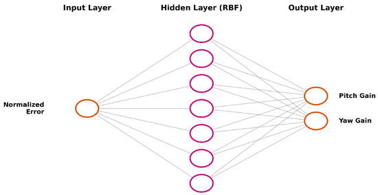
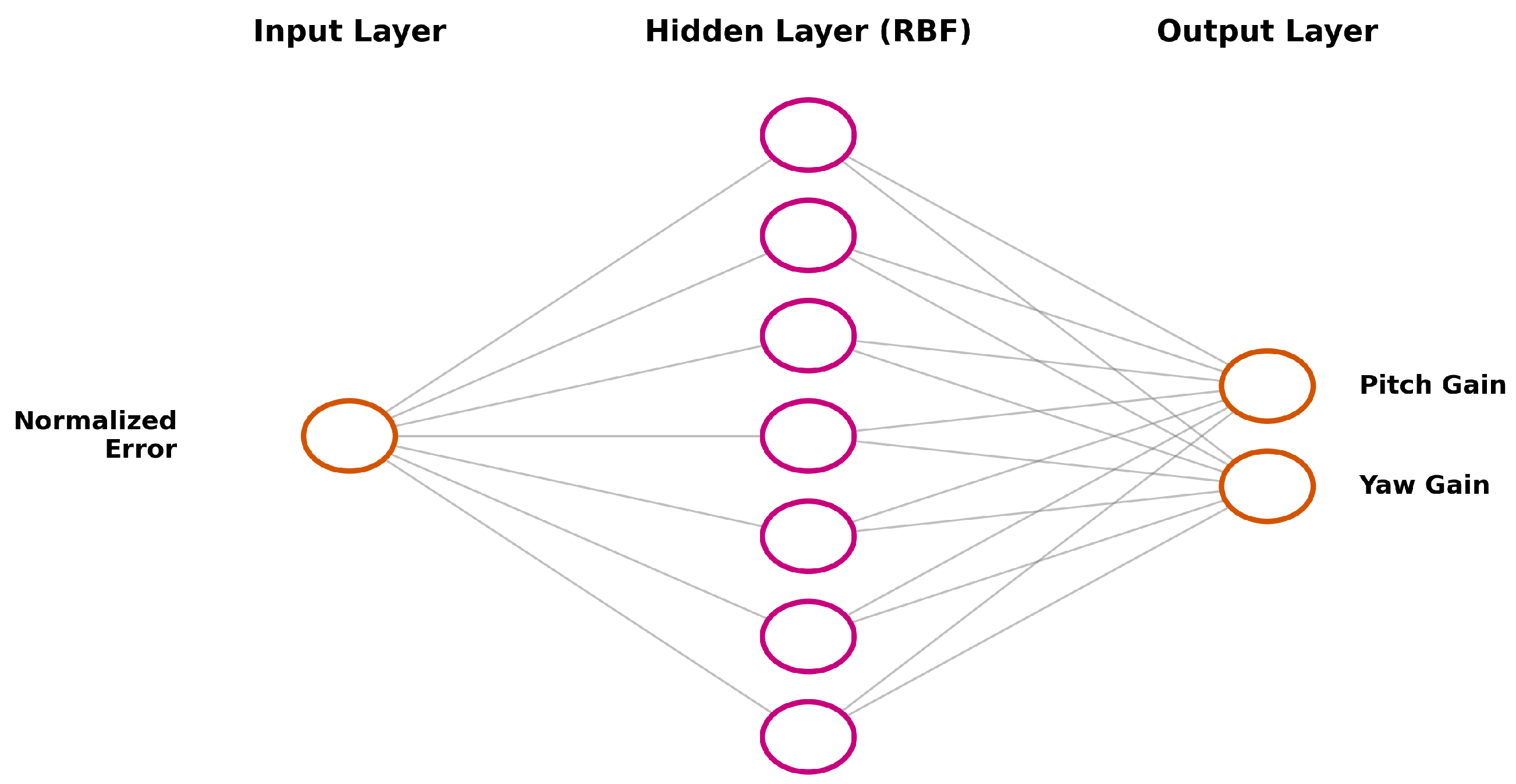
where $w_{i,j}$ are the output weights. The internal structure of this neural network is depicted in Figure 2.

Figure 2. Architecture of the RBF Neural Network used for online tuning. The network takes the normalized tracking error ($x_{in}$) as input, processes it through 7 Gaussian hidden neurons, and outputs the adaptive observer gains for Pitch (${\theta }_p$) and Yaw (${\theta }_y$).

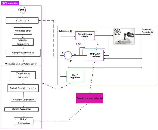
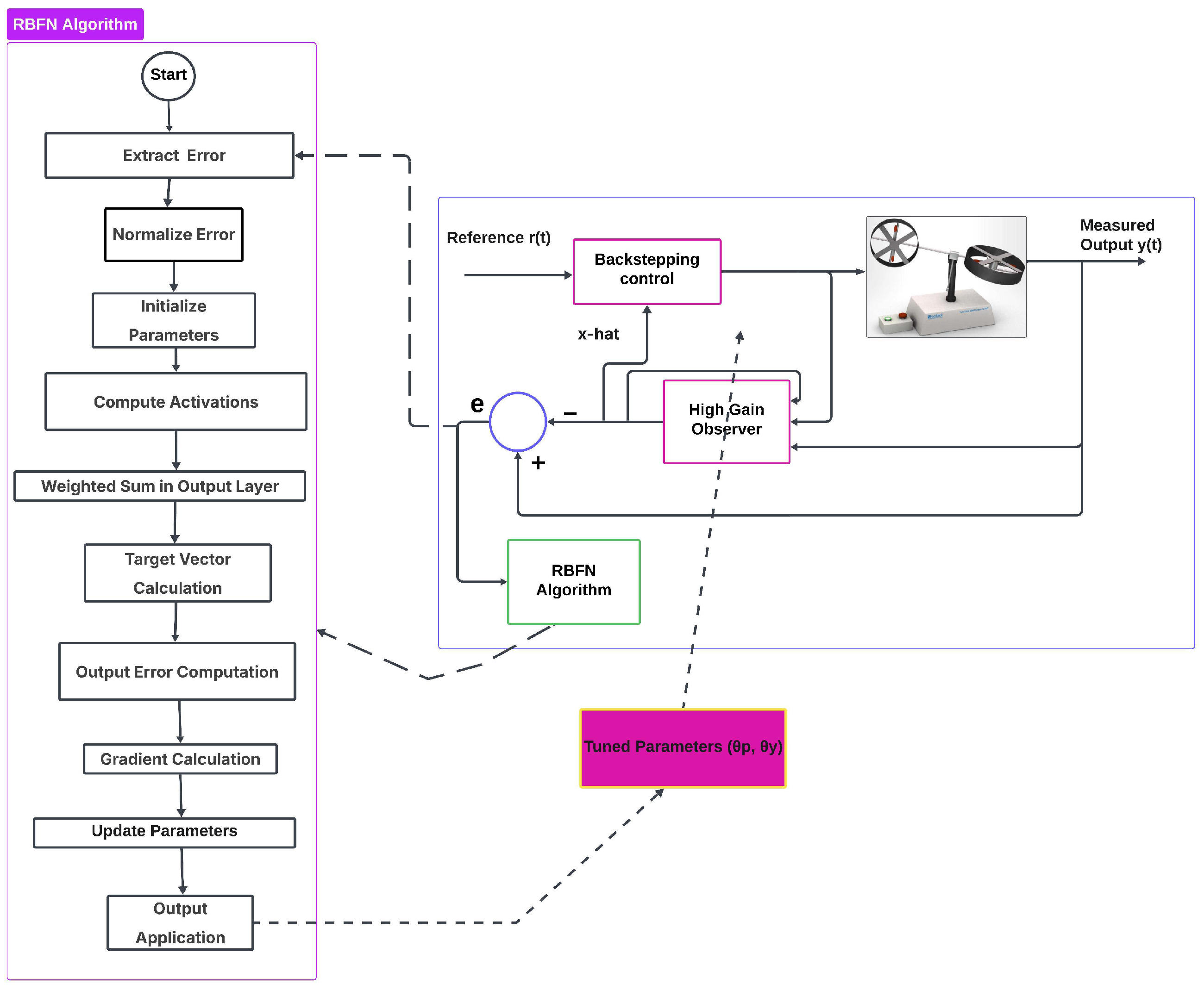
To visualize how this adaptive tuning mechanism interacts with the backstepping controller and the observer in the real-time loop, the complete integration scheme is illustrated in Figure 3.

Figure 3. Flowchart of the RBFNN-HGO tuning mechanism and its integration with the TRMS control loop.

2.4.2. Safety Scaling and Output Smoothing

To guarantee that the observer gains remain within a safe, physical range on the hardware (avoiding the peaking phenomenon), the raw network outputs $y_{net}$ are processed through a final scaling layer:

$${\theta }_{p,raw}=1+4\left({\displaystyle \frac{tanh\left(y_{net,1}\right)+1}{2}}\right)\in [1,5]$$

(63)

$${\theta }_{y,raw}=0.5+1.5\left({\displaystyle \frac{tanh\left(y_{net,2}\right)+1}{2}}\right)\in [0.5,2]$$

(64)

Additionally, a discrete-time low-pass filter is applied to prevent abrupt changes in the observer dynamics:

$$\Theta \left(k\right)=0.8\Theta (k-1)+0.2{\Theta }_{raw}\left(k\right)$$

(65)

where $\Theta ={[{\theta }_p,{\theta }_y]}^T$.

2.4.3. Learning Algorithm

The training process uses a target-based gradient descent approach. The target vector is designed to increase the observer gain when the error is large (to force convergence) and decrease it when the error is small (to reduce noise sensitivity):

$$\mathrm{target}\left(k\right)=\left[\begin{array}{c}1+tanh\left(e\right(k\left)\right)\\ 0.5(1+tanh(e\left(k\right)\left)\right)\end{array}\right]$$

(66)

The parameter gradients for the weights (w), centers (c), and widths ($\sigma$) are derived via the chain rule to minimize the instantaneous cost function $J={\displaystyle \frac{1}{2}}\sum {(targe{t}_j-y_{net,j})}^2$. The complete computational procedure is detailed in Algorithm 1.

Algorithm 1 Online HGO Tuning via RBF Neural Network

Require:  Estimation error $e\left(k\right)$, Previous gains $\Theta (k-1)$, RBF parameters ($c,\sigma ,w$) Ensure:  Tuned HGO parameters $\Theta \left(k\right)={[{\theta }_p,{\theta }_y]}^T$   1: Input Pre-processing:   2: $x_{in}\leftarrow tanh(e\left(k\right)/2)$              ▹ Normalize input to [−1, 1]   3: Forward Pass (RBF):   4: for $i=1$ to N do   5:        ${\varphi }_i\leftarrow exp(-{(x_{in}-c_i)}^2/\left(2{\sigma }_i^2\right))$   6: end for   7: $y_{net}\leftarrow \sum w_i{\varphi }_i$   8: Target Generation:   9: $Target\leftarrow {[1+tanh\left(e\left(k\right)\right);0.5(1+tanh\left(e\left(k\right)\right))]}^T$ 10: Parameter Update (Gradient Descent): 11: Compute Output Error: $E\leftarrow Target-y_{net}$ 12: Update $w\leftarrow w+\eta ·E·\varphi$ 13: Update $c\leftarrow c+\eta ·E·w·\varphi ·(x_{in}-c)/{\sigma }^2$ 14: Output Smoothing & Scaling: 15: ${\theta }_p\leftarrow 1+4\left(0.5(tanh\left(y_{net,1}\right)+1)\right)$ 16: ${\theta }_y\leftarrow 0.5+1.5\left(0.5(tanh\left(y_{net,2}\right)+1)\right)$ 17: $\Theta \left(k\right)\leftarrow 0.8\Theta (k-1)+0.2{[{\theta }_p,{\theta }_y]}^T$ 18: return  $\Theta \left(k\right)$

3. Results and Discussion

3.1. Experimental and Simulation Setup

To bridge the gap between theory and practice, the proposed control strategy was validated through both numerical simulation and physical implementation.

Simulation Platform: Initial validation was performed in MATLAB/Simulink (2014a) (The MathWorks, Inc., Natick, MA, USA). The full nonlinear model (Equation (2)) was simulated using the ode1 (Euler) fixed-step solver with a step size of 0.001s to match the hardware sampling rate.

Experimental Hardware: The physical implementation utilizes a Hardware-in-the-Loop (HIL) architecture, as detailed below:

• Hardware Interface: The TRMS rig is interfaced via an Advantech PCI-1711 data acquisition card. This card features 12-bit Analog Output (DAC) channels to drive the DC motors and high-speed digital inputs to read the optical encoders (2000 pulses/rev) for pitch and yaw angles.
• Real-Time Kernel: The control algorithms were compiled using the Simulink Real-Time Windows Target kernel, allowing the PC to execute the control law deterministically at 100 Hz ($T_s=0.01$ s).
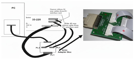
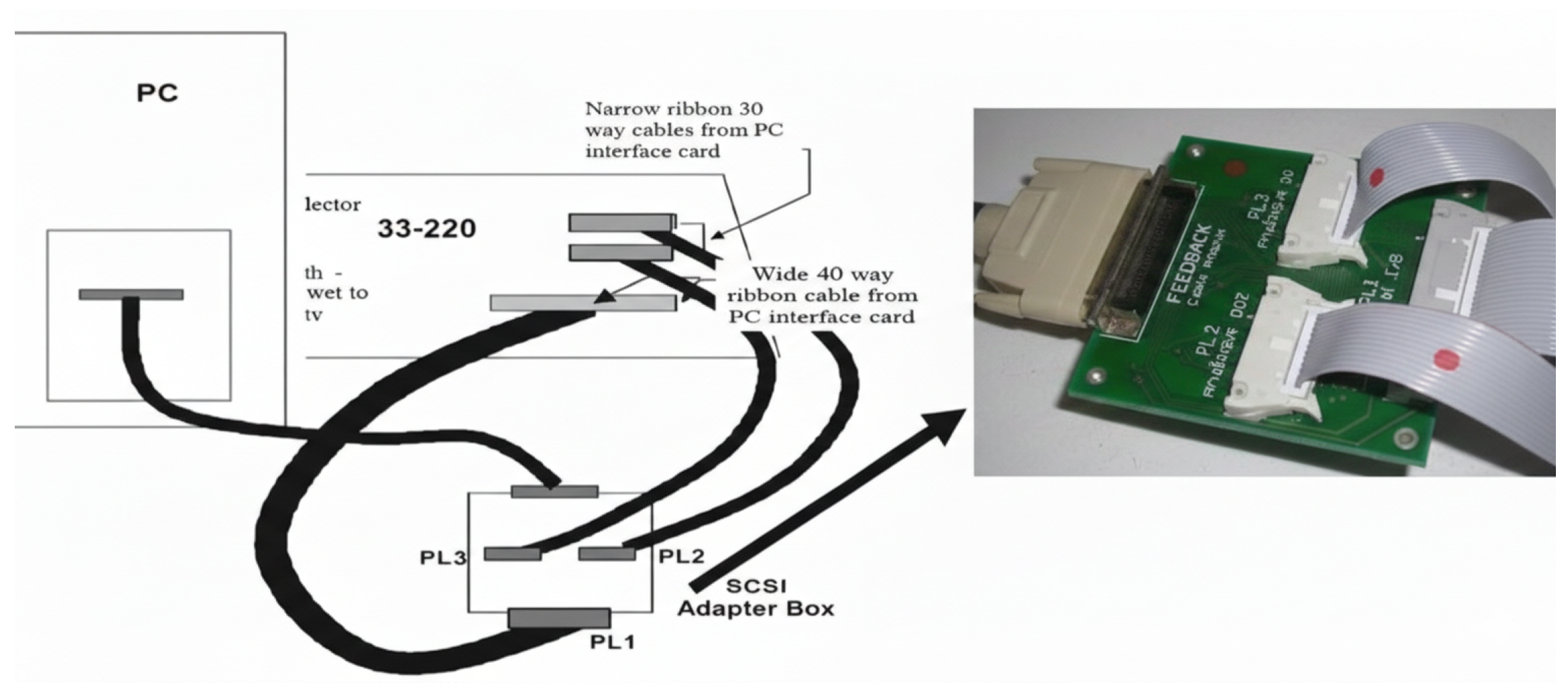
• Signal Conditioning: A SCSI adapter box interfaces the PCI card to the TRMS base unit, routing voltage commands ($U_1,U_2$) and sensor feedback ($\psi ,\varphi$).

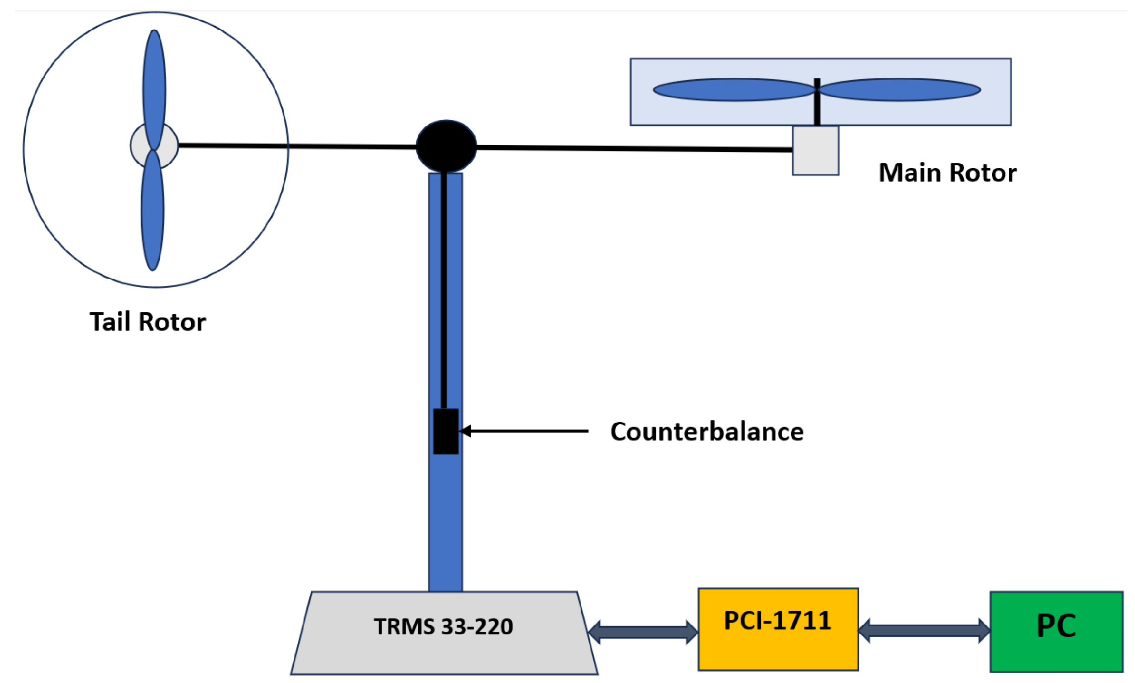
Figure 4 illustrates the schematic of the hardware-in-the-loop connection between the control PC and the TRMS unit.

Figure 4. Experimental hardware interface: detailed connection schematic showing the signal flow between the PC, the Advantech PCI-1711 data acquisition card, and the TRMS base unit. Arrows indicate the direction of signal transmission.

To ensure a fair comparison between the controllers, a standardized tuning protocol was followed. The Baseline HGO gains were manually tuned to the maximum possible value ($\theta \approx 3$) before noise-induced vibration became detrimental to the mechanical structure. The RBF-HGO was initialized with these same conservative base values. This ensures that any performance improvement is solely due to the RBF network’s ability to dynamically increase the gain during transients without causing instability.

3.2. Simulation Results

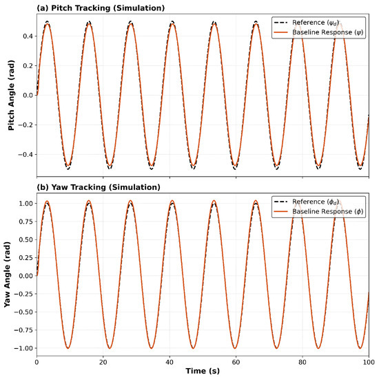
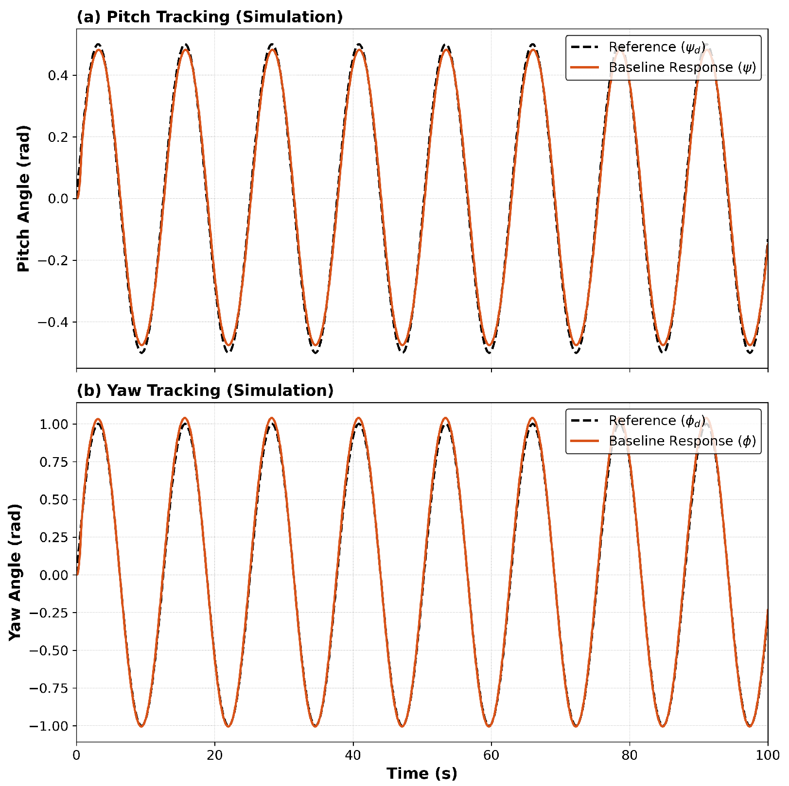
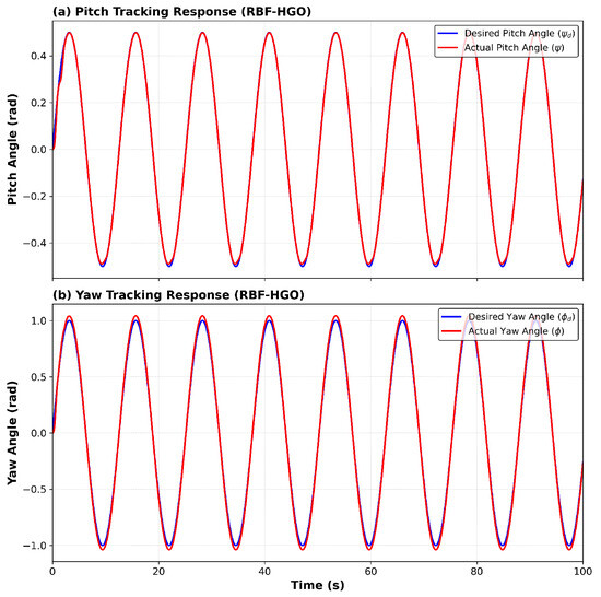
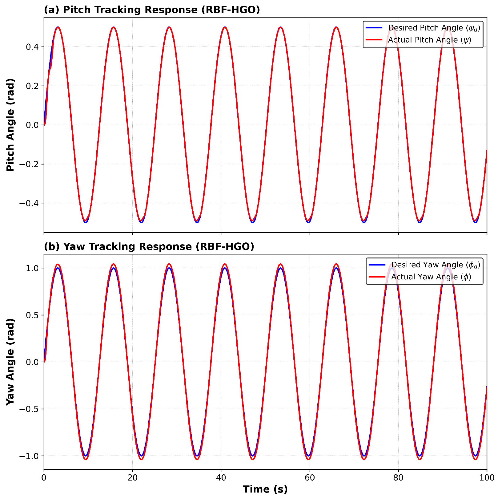
We first simulated the validation of the control strategies. Figure 5 shows that Baseline HGO recorded stability in tracking performance. Figure 6 shows the working performance of the proposed RBFN-HGO, which shows a significant improvement.

Figure 5. Simulated tracking performance of the standard HGO: (a) Pitch axis tracking; (b) Yaw axis tracking.

Figure 6. Simulated tracking performance of the RBFNN-enhanced HGO.

3.3. Experimental Results and Discussion

After that, the controller was put to trial on real hardware. The TRMS set up was used to conduct the experiments. The task was to compare the proposed RBFNN-tuned HGO and the standard fixed gain-tuned observer, also known as the Baseline HGO.

3.3.1. Performance of the Baseline HGO Controller

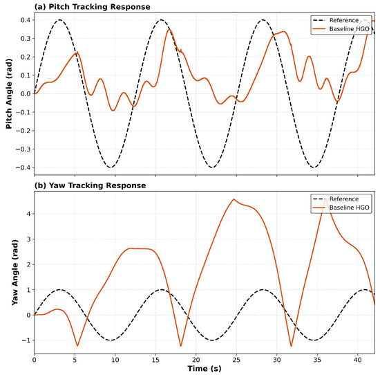
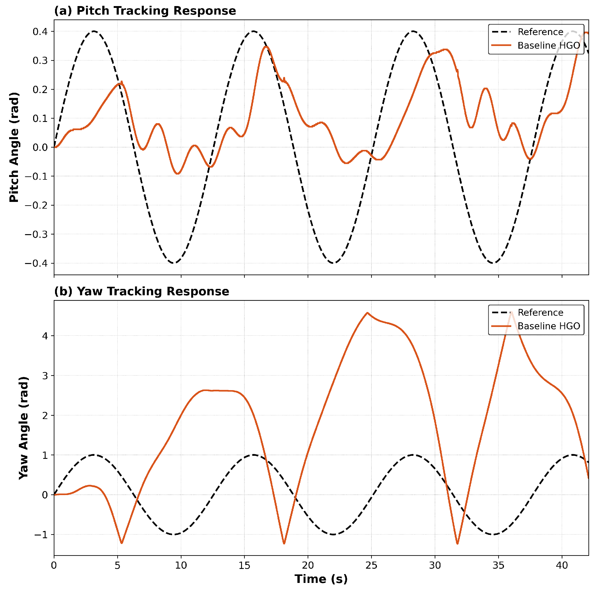
When transitioning from simulation into the implementation of the hardware, the shortcoming of the traditional approach was clear. The behavior is seen as shown in Figure 7. The Baseline HGO controller malfunctioned completely with the resultant destabilization of the whole system. It was therefore stopped to avoid any possible damage to the equipment.

Figure 7. Real-time tracking performance of the standard HGO, showing unstable behavior.

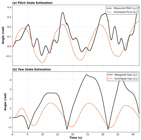
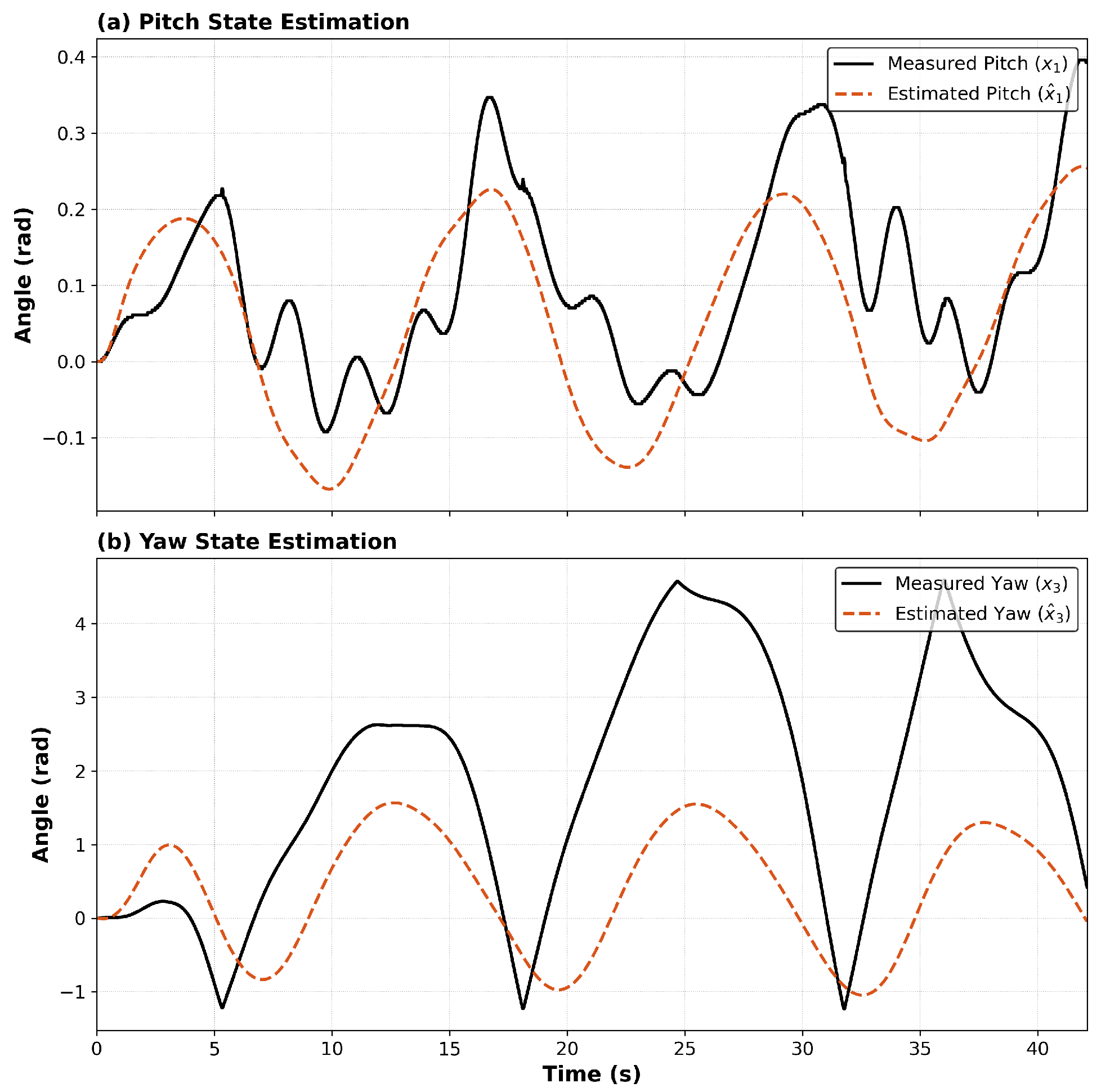
Figure 8 shows the root cause of this failure. The state estimation from the baseline HGO was clearly very poor. The estimates made by the observer quickly diverged from the actual measured angles, so that the observer was providing erroneous estimated states to the backstepping controller. These inaccurate states directly caused the instability of the system.

Figure 8. Real-time observer failure (Baseline).

3.3.2. Performance of the Proposed RBFNN-HGO Controller

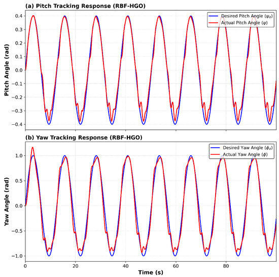
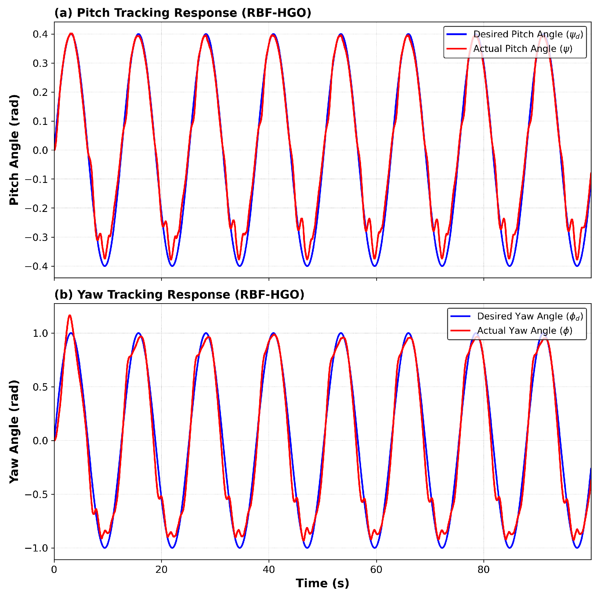
In contrast to the baseline results, the RBFNN-HGO controller displayed an improved and robust performance under the same experimental conditions. The controller maintained accurate and stable control of the reference trajectories over the entire duration of the experiment, as shown in Figure 9.

Figure 9. Real-time tracking performance of the RBFNN-enhanced HGO.

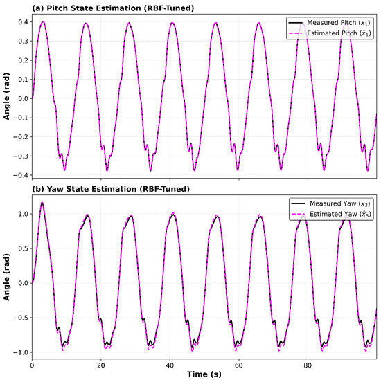
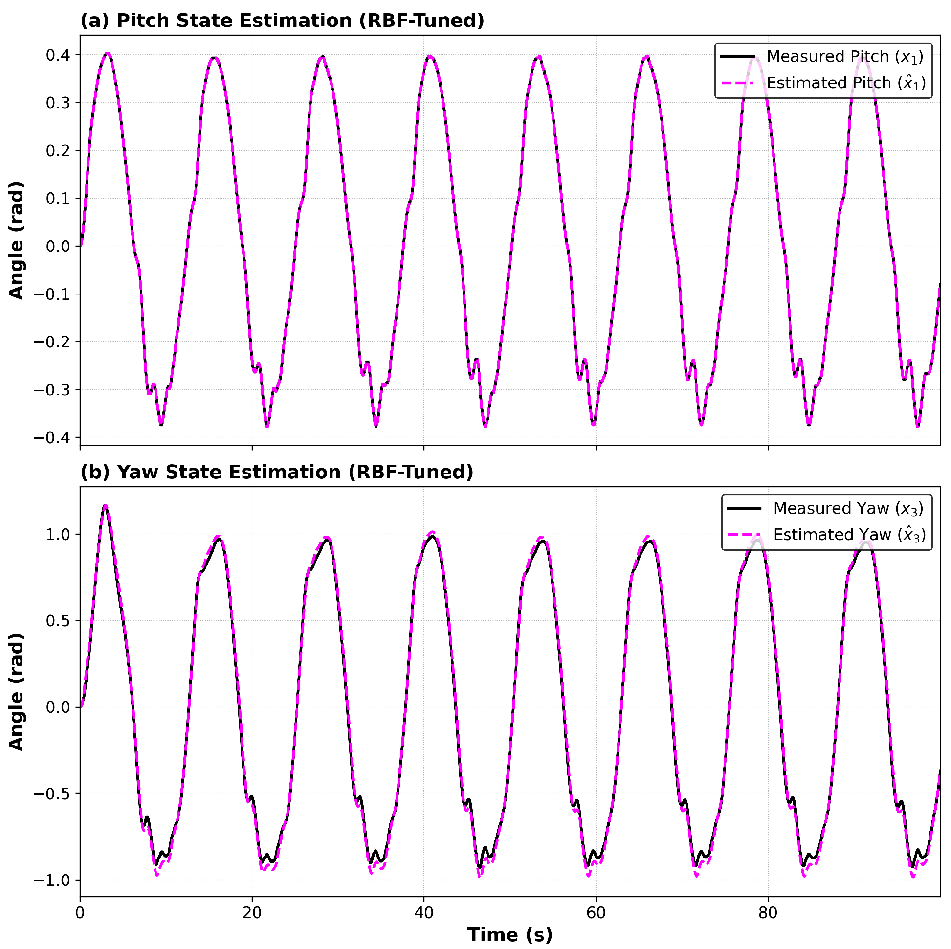
To explain the cause of this performance improvement, Figure 10 illustrates the high-fidelity estimation capabilities of the RBFNN-tuned observer. As the graph shows, the estimated angles of pitch ($\widehat{\psi }$) and yaw ($\widehat{\varphi }$) converge rapidly to the actual measured angles ($\psi ,\varphi$). This accurate state estimation is the cornerstone of the system’s stability, ensuring that the backstepping controller receives precise feedback despite model uncertainties.

Figure 10. Observer angle performance: comparison of estimated states ($\widehat{x}$) vs. measured states (x) using the RBFNN-tuned HGO.

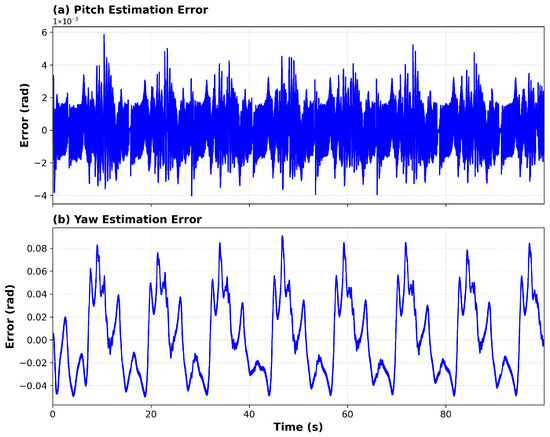
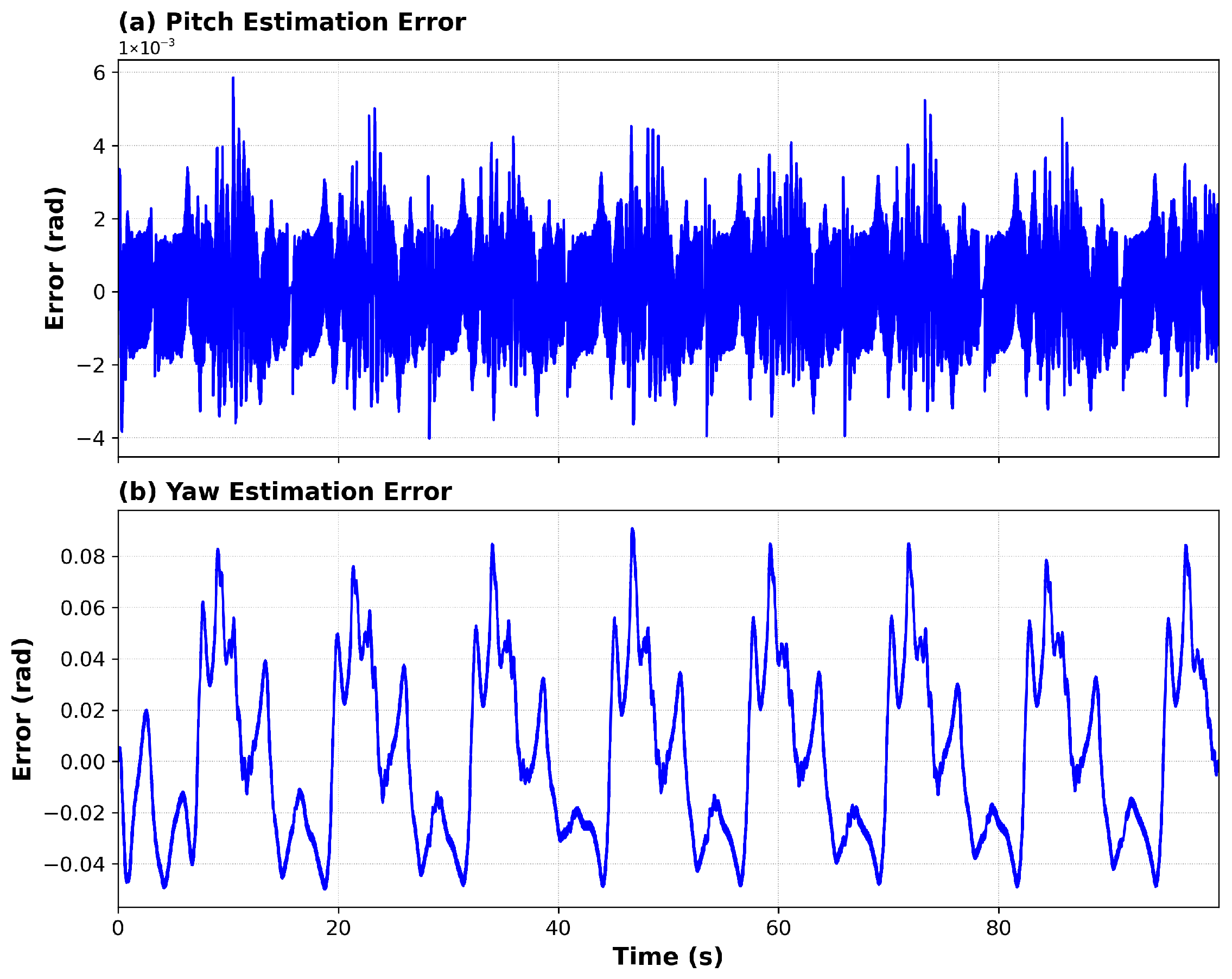
To further quantify this precision, Figure 11 presents the observer estimation error. Unlike the baseline observer, which diverged, the RBF-tuned observer maintains the estimation error within a very narrow bound (pitch error $<\pm 0.005$ rad), effectively rejecting measurement noise.

Figure 11. Evolution of the observer estimation error: (a) Pitch axis estimation error $e_{\psi }$; (b) Yaw axis estimation error $e_{\varphi }$, showing bounded convergence.

3.3.3. Analysis of Adaptive Gains

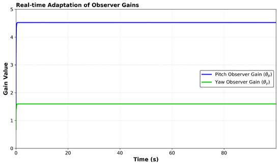
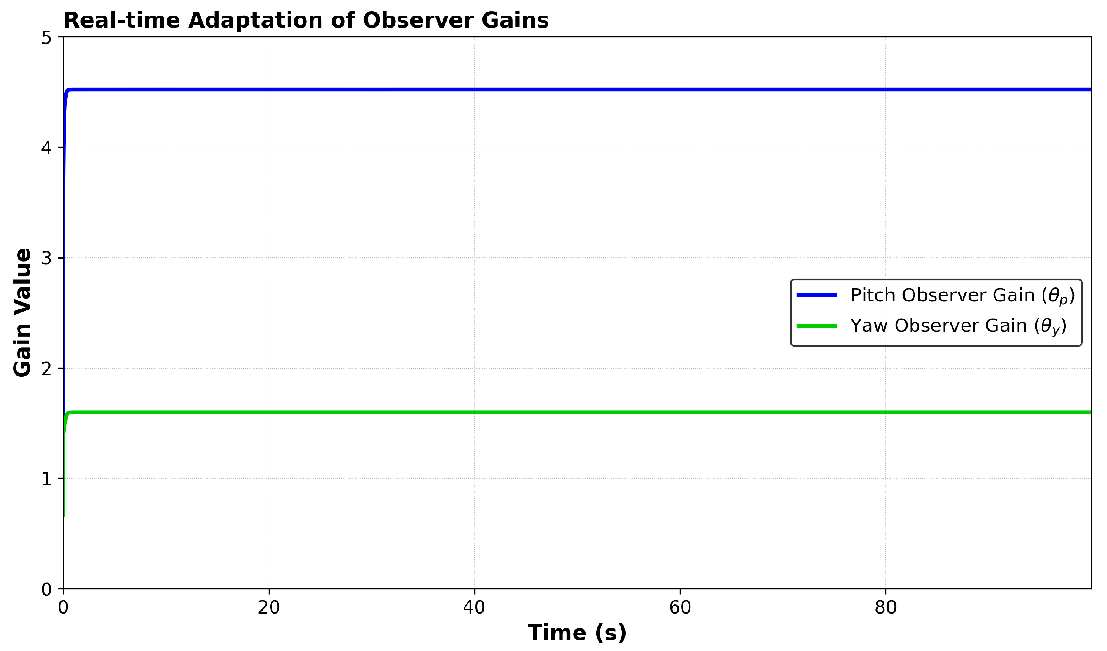
The mechanism behind this stability is revealed in the time evolution of the adaptive gains. Figure 12 illustrates how the RBF network tunes ${\theta }_p$ and ${\theta }_y$ in real time. The gains do not drift to infinity; instead, the pitch gain settles rapidly around 4.5, while the yaw gain stabilizes at a lower value (approx. 1.6). This confirms that the network successfully identified the “sweet spot” where the gain is high enough to track states but low enough to avoid noise amplification.

Figure 12. Real-time adaptation of the High-Gain Observer parameters.

3.3.4. Comparative Analysis and Quantitative Evaluation

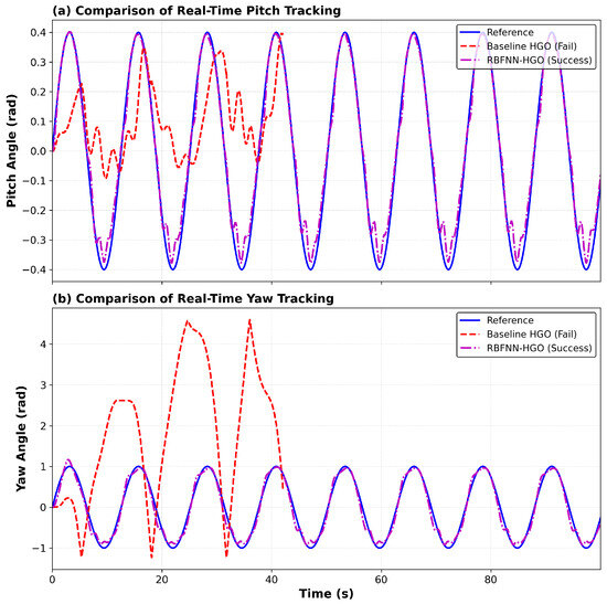
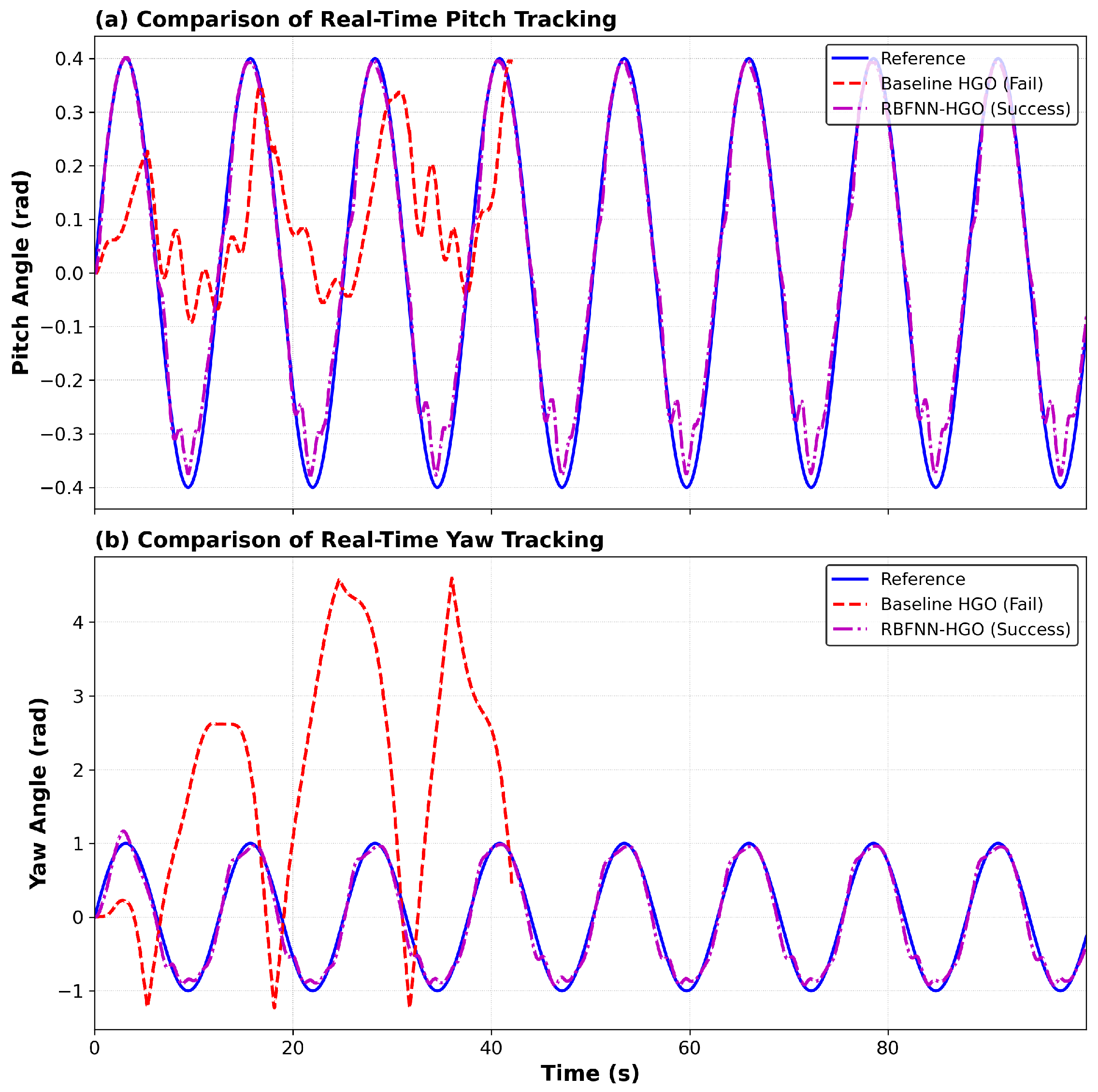
A direct overlay of the two controllers’ tracking responses is presented in Figure 13. This visual comparison definitively highlights the superiority of the proposed method: the Baseline HGO (red, dashed line) exhibits severe oscillations and failure, whereas the RBFNN-HGO (magenta, dash-dot line) adheres tightly to the reference trajectory (blue).

Figure 13. Comparative real-time tracking performance. The Baseline HGO (red) fails, while the proposed RBFNN-HGO (magenta) robustly tracks the reference.

The visual evidence is substantiated by the quantitative comparison in Table 1. The RBFNN-HGO reduced the Root Mean Square Error (RMSE) by **85.0%** in the pitch axis and **95.8%** in the yaw axis compared to the baseline.

Table 1. Quantitative comparison of controller performance in real-time tracking.

Performance Metric	Baseline HGO	RBFNN-HGO	Improvement (%)
RMSE (Pitch) [rad]	0.2571	0.0385	85.0%
RMSE (Yaw) [rad]	2.5624	0.1080	95.8%
ITAE (Pitch) [rad·s]	1990.24	1486.68	25.3%
ITAE (Yaw) [rad·s]	21281.99	4077.79	80.8%
Control Energy (Pitch) [V2·s]	82.83	3636.53	-
Control Energy (Yaw) [V2·s]	352.25	1119.65	-

4. Conclusions

This study addresses the critical challenge of bridging the gap between simulation and real-time implementation for nonlinear control systems. We demonstrated that while a conventional backstepping controller coupled with a fixed-gain High-Gain Observer (HGO) exhibits excellent tracking in simulation, it fails to stabilize the physical Twin Rotor MIMO System (TRMS). This failure is attributed to the observer’s sensitivity to measurement noise and the peaking phenomenon when high gains are applied to a real-world plant with unmodeled dynamics.

To overcome this limitation, a novel adaptive framework employing a Radial Basis Function (RBF) Neural Network was introduced to tune the observer gains in real time. Experimental results validate the efficacy of this approach; the adaptive observer not only restores closed-loop stability but also significantly enhances tracking precision, reducing the Root Mean Square Error (RMSE) by 85.0% in the pitch axis and 95.8% in the yaw axis compared to the baseline configuration.

These findings substantiate that online adaptive tuning of observer gains is a decisive strategy for reconciling the disparity between theoretical design and physical constraints in complex nonlinear systems. Future work will focus on extending this adaptive framework to reject abrupt external disturbances, such as wind gusts, and investigating finite-time convergence properties to further enhance system robustness.

References

- Ezekiel, D.M.; Samikannu, R.; Matsebe, O. Pitch and yaw angular motions (rotations) control of the 1-DOF and 2-DOF TRMS: A survey. Arch. Comput. Methods Eng. 2021, 28, 1449–1458. [Google Scholar] [CrossRef] [Scilit]
- Ahmed, U.; Ahmed, W. Evaluation and Comparison of TRMS Performance for Classical and Optimal Control Strategies. In 2023 International Conference on Robotics and Automation in Industry (ICRAI); IEEE: Piscataway, NJ, USA, 2023; pp. 1–7. [Google Scholar]
- Palepogu, K.R.; Mahapatra, S. Design of sliding mode control with state varying gains for a Benchmark Twin Rotor MIMO System in Horizontal Motion. Eur. J. Control 2024, 75, 100909. [Google Scholar] [CrossRef] [Scilit]
- Kacimi, A.; Senoussaoui, A. Feedback Linearization Controller with Thau Observer. J. Autom. Mob. Robot. Intell. Syst. 2025, 19, 66–74. [Google Scholar] [CrossRef] [Scilit]
- Kokotovic, P.V. The joy of feedback: Nonlinear and adaptive. IEEE Control Syst. Mag. 1992, 12, 7–17. [Google Scholar]
- Krstic, M.; Kokotovic, P.V.; Kanellakopoulos, I. Nonlinear and Adaptive Control Design; John Wiley & Sons: New York, NY, USA, 1995. [Google Scholar]
- Noordin, A.; Basri, M.A.M.; Othman, S.M. Trajectory Tracking of Autonomous Mobile Robot via Backstepping Control Approach. In 2025 IEEE International Conference on Automatic Control and Intelligent Systems (I2CACIS); IEEE: Piscataway, NJ, USA, 2025; pp. 152–157. [Google Scholar]
- El Haissouf, M.; El Haroussi, M.; Ba-Razzouk, A.; Bensaid, M. Processor In the Loop implementation of two stages Backstepping control strategy. EPJ Web Conf. 2025, 330, 02009. [Google Scholar] [CrossRef] [Scilit]
- Purwar, S. Adaptive Terminal Sliding Mode Disturbance Observer Augmented Backstepping Integral Sliding Mode Control for Twin Rotor MIMO System. In 2024 35th Irish Signals and Systems Conference (ISSC); IEEE: Piscataway, NJ, USA, 2024; pp. 1–6. [Google Scholar]
- Tao, X.; Liu, K.; Yang, J.; Chen, Y.; Chen, J.; Zhu, H. Sliding mode backstepping control of excavator bucket trajectory synovial in particle swarm optimization algorithm and neural network disturbance observer. Actuators 2025, 14, 9. [Google Scholar] [CrossRef] [Scilit]
- Khalil, H.K. High-gain observers in feedback control: Application to permanent magnet synchronous motors. IEEE Control Syst. Mag. 2017, 37, 25–41. [Google Scholar]
- Farza, M.; Chehaïbi, O.; Saïd, S.H.; M’Saad, M. Design of a Saturated Filtered High Gain Observer for a Class of Disturbed Nonlinear Systems. Int. J. Robust Nonlinear Control 2025, 35, 6789–6814. [Google Scholar] [CrossRef] [Scilit]
- Mousavi, S.; Guay, M. A low-power multi-high-gain observer design for a class of nonlinear systems. IEEE Trans. Autom. Control 2024, 69, 6405–6412. [Google Scholar] [CrossRef] [Scilit]
- Mahmod, R.A.; Kadhima, R.A.; Nawfal, M.; Al-Khazraji, H. High Gain Observer Based Backstepping Control Design for Nonlinear Single-Axis Driven Systems. Int. J. Robot. Control Syst. 2025, 5, 1886–1899. [Google Scholar] [CrossRef] [Scilit]
- Jafari, R.; Jafari, A.H. Nonlinear Adaptive control with High-Gain Observer. In 2025 International Conference on Control, Automation and Diagnosis (ICCAD); IEEE: Piscataway, NJ, USA, 2025; pp. 1–8. [Google Scholar]
- Alai, H.; Zemouche, A.; Rajamani, R. Vehicle trajectory estimation using a high-gain multi-output nonlinear observer. IEEE Trans. Intell. Transp. Syst. 2024, 25, 5733–5742. [Google Scholar] [CrossRef] [Scilit]
- Tufenkci, S.; Alagoz, B.B.; Kavuran, G.; Yeroglu, C.; Herencsar, N.; Mahata, S. Implementations of TD3 and DDPG Reinforcement Learning Techniques for Tuning PID Controller of TRMS System. J. Syst. Sci. Syst. Eng. 2025, 34, 1–20. [Google Scholar] [CrossRef] [Scilit]
- Kacimi, A.; Beloufa, A.; Tahraoui, S.; Senoussaoui, A. Optimized T-S fuzzy logic 2 enhanced observer for twin rotor backstepping control. Electroteh. Electron. Autom. EEA 2025, 73, 96–103. [Google Scholar] [CrossRef] [Scilit]
- Haykin, S. Neural Networks and Learning Machines, 3rd ed.; Prentice Hall: Upper Saddle River, NJ, USA, 2009. [Google Scholar]
- Kumar, R. Recurrent context layered radial basis function neural network for the identification of nonlinear dynamical systems. Neurocomputing 2024, 580, 127524. [Google Scholar] [CrossRef] [Scilit]
- Kapnopoulos, A.; Kazakidis, C.; Alexandridis, A. Quadrotor trajectory tracking based on backstepping control and radial basis function neural networks. Results Control Optim. 2024, 14, 100335. [Google Scholar] [CrossRef] [Scilit]
- Feedback Instruments. Twin Rotor MIMO System Control Experiments Manual 33-949S. 2006. Available online: http://www.cpdee.ufmg.br/~palhares/33-942rotor.pdf (accessed on 9 December 2025).
- Keighobadi, J.; Mehrjouyan, A.; Alfi, A. Efficient learning control of uncertain nonlinear systems with input constraints: A disturbance observer-based neural network approach. Int. J. Dyn. Control 2024, 12, 3392–3406. [Google Scholar] [CrossRef] [Scilit]
- Senoussaoui, A.; Chenafa, M.; Kacimi, A.; Ne, R.H. Neural Network NARMA L-2 control of a twin rotor MIMO system. In Proceedings of the 2019 International Conference on Advanced Electrical Engineering (ICAEE’19), Algiers, Algeria, 19–21 November 2019. [Google Scholar]
- Senoussaoui, A.; Chenafa, M.; Ahraoui, M.; Kacimi, A.; Houcine, R. LQGi/LTR controller with integrators and feedforward controller applied to a twin rotor MIMO system. Przegląd Elektrotechniczny 2021, 97, 1–6. [Google Scholar]
- Nguyen, N.K.; Bui, Q.V.B.; Nguyen, Q.H.; Luong, T.G.; Nguyen, L.N. Adaptive fuzzy-neural network effectively disturbance compensate in sliding mode control for dual arm robot. EUREKA Phys. Eng. 2024, 2, 79–93. [Google Scholar] [CrossRef] [Scilit]
- Bornard, G.; Hammouri, H. A high gain observer for a class of uniformly observable systems. In Proceedings of the 30th IEEE Conference on Decision and Control, Brighton, UK, 11–13 December 1991; pp. 1494–1496. [Google Scholar]
- Razmjooei, H.; Palli, G.; Abdi, E.; Terzo, M.; Strano, S. Design and experimental validation of an adaptive fast-finite-time observer on uncertain electro-hydraulic systems. Control Eng. Pract. 2023, 131, 105391. [Google Scholar] [CrossRef] [Scilit]
- Lu, H.; Li, J.; Li, S.; Wang, S.; Xiao, Y. Finite-time extended state observer enhanced nonsingular terminal sliding mode control for buck converters in the presence of disturbances: Design, analysis and experiments. Nonlinear Dyn. 2024, 112, 7113–7127. [Google Scholar] [CrossRef] [Scilit]
- Li, M.; Du, J. Finite-Time Observer Based Prescribed Performance Robust Control for Position Stabilization of Offshore Gangway Ends. Int. J. Robust Nonlinear Control 2025, 35, 2235–2245. [Google Scholar] [CrossRef] [Scilit]
- Khalil, H.K.; Grizzle, J.W. Nonlinear Systems, 3rd ed.; Prentice Hall: Upper Saddle River, NJ, USA, 2002. [Google Scholar]
- Vidyasagar, M. Nonlinear Systems Analysis, 2nd ed.; Prentice Hall: Englewood Cliffs, NJ, USA, 1993. [Google Scholar]
- Moody, J.; Darken, C.J. Fast learning in networks of locally-tuned processing units. Neural Comput. 1989, 1, 281–294. [Google Scholar] [CrossRef] [Scilit]
Disclaimer/Publisher’s Note: The statements, opinions and data contained in all publications are solely those of the individual author(s) and contributor(s) and not of MDPI and/or the editor(s). MDPI and/or the editor(s) disclaim responsibility for any injury to people or property resulting from any ideas, methods, instructions or products referred to in the content. |
© 2026 by the authors. Licensee MDPI, Basel, Switzerland. This article is an open access article distributed under the terms and conditions of the Creative Commons Attribution (CC BY) license.