


Abstract
GPU LDPC latency comparisons across implementations are challenging due to variations in decoder schedules, batch granularity, and timing boundaries. Batch completion was characterized for FP32-layered and flooding decoders on a GPU, considering block acquisition, matched outcomes, and three timing boundaries. The schedule study included 600,000 observations. Flooding exhibited higher P50 and P99 in 15 full-boundary matched-cap comparisons, while and did not display uniform schedule ordering. For words satisfying the syndrome under both schedules, layered decoding achieved first satisfaction earlier in every estimable 2- and 4-dB cell. Layered endpoint levels varied among full, decode-only, and transfer-only boundaries. Over six sessions, full-boundary increased by 234.7 μs from batch 64 to 128 (pointwise descriptive 95% percentile interval, 196.1–281.5 μs), which contrasted with two other designs. These results pertain to a single dynamically clocked Windows Subsystem for Linux 2 (WSL2) GPU and do not establish fixed-clock or cross-platform behavior, radio-interface latency, causal attribution, or worst-case bounds.
1. Introduction
Fifth-generation (5G) New Radio (NR) supports services with different throughput, reliability, and delay requirements. Ultra-reliable low-latency communication (URLLC) is a prominent example, but its service latency includes radio-interface, protocol, transport, and application processing rather than a single decoder call [1,2]. Decoder measurements can therefore inform a physical-layer budget without demonstrating URLLC compliance.
Low-density parity-check (LDPC) codes, introduced by Gallager [3], protect the NR data channel [4]. Their sparse quasi-cyclic graphs expose parallelism that maps naturally to graphics processing units (GPUs). Existing GPU implementations demonstrate standards-oriented decoding, high throughput, and integration with virtualized radio-access software [5,6,7,8,9,10]. Cross-platform results also show that data movement and workload granularity affect accelerator performance [11]. Reported latency values nevertheless depend on the graph, precision, stopping rule, batch definition, schedule, and timed software boundary.
Real-time GPU research examines scheduling, interference, resource isolation, and analyzable execution. TimeGraph controls GPU work at the driver level, whereas GPUSync coordinates accelerator access in multicore, multi-GPU systems [12,13]; Gheibi Fetrat et al. survey the broader architectural and scheduling constraints [14]. The present study instead characterizes the empirical distribution of one declared decoder-batch boundary without an intentionally co-scheduled GPU workload. The measurements are not response-time bounds or schedulability tests.
The studies reviewed here do not jointly provide three forms of evidence for one controlled decoder setting: whether schedule differences persist in both latency endpoints and matched decoding outcomes, how those endpoints depend on the declared software timing boundary, and whether an observed batch-tail direction recurs across acquisition sessions. This empirical gap is narrower than the problem addressed by real-time schedulability research. It concerns measured decoder-batch distributions rather than worst-case response-time or interference guarantees.
The primary comparisons evaluate schedule latency, matched schedule outcomes, three timing boundaries, and the batch-64-to-128 direction across six acquisition sessions. Sensitivity analyses vary the algorithm, stopping rule, input mode, channel condition, graph, lifting size, and operating state. Block-placement and CUDA Profiling Tools Interface (CUPTI) records provide supplementary diagnostic evidence: they constrain interpretation but do not identify a hardware mechanism.
The study addresses four questions:
- RQ1.
- How do P50, P99, absolute P99–P50 separation , and the P99-to-P50 ratio differ between the tested layered and flooding implementations at the tested batches and fixed iteration caps?
- RQ2.
- How do the two implementations compare in information-bit error rate (BER), information-word block error rate (BLER), final syndrome success, and first syndrome satisfaction when they decode the same codewords and noise?
- RQ3.
- For the layered implementation, how do these endpoints differ among the full, decode-only, and equal-volume transfer-only boundaries, and does the batch-64-to-128 direction recur across acquisition sessions?
- RQ4.
- How sensitive are the measured endpoints to algorithm, channel, input, graph, lifting size, stopping rule, and starting state?
The study makes three empirical and methodological contributions. Methodologically, it applies established P50, P99, , and endpoints within explicitly declared software boundaries and uses paired block-level resampling to preserve the acquisition-block structure in contrasts. Comparatively, it relates schedule latency to outcomes from matched codeword/noise pairs rather than assuming that equal iteration caps imply equal decoding behavior. Empirically, it finds under the tested conditions that flooding is higher at P50 and P99 in every same-cap schedule cell, whereas and have no uniform schedule ordering, and that the layered batch-64-to-128 direction differs across experimental designs.
Internal checks establish consistency among the encoded words, compiled graph, CPU reference, and GPU outputs; they are not an independent 3GPP conformance certification. The scope is synchronous decoder-batch completion for the tested FP32 implementations on one dynamically clocked RTX 4070 Ti SUPER under WSL2. Native Linux, a second GPU, fixed clocks, and hardware performance counters were unavailable, so the results do not support platform-wide generalization or causal microarchitectural attribution.
2. Background and Related Work
2.1. NR LDPC Graphs and Min-Sum Decoding
Irregular LDPC constructions can approach channel capacity while retaining sparse-graph decoding [15]. NR defines two quasi-cyclic base graphs for different information-block and rate regimes [4]. The primary configuration uses Base Graph 1 (BG1), lifting size , and lifting-set index . We selected because it is the largest standardized lifting size, provides a high-workload case on the available device, and matches the baseline scaling configuration. It yields 26,112 internal values and 121,344 lifted edges per codeword. BG1 contains 46 base-graph rows, 68 columns, and 316 nonzero circulant permutation submatrices. Its systematic region has bits, including the first punctured positions. Controls use BG1 at and BG2 at ; they test sensitivity to lifting size and topology but do not establish representativeness across all NR configurations.
Let denote the channel log-likelihood ratio (LLR), a check-to-variable message, the variables adjacent to check m, and the checks adjacent to variable n. For extrinsic values , the min-sum check rule is
Here, for and otherwise, matching the two-valued sign used by both kernels. The corresponding sum–product magnitude is
It does not exceed the minimum magnitude used by min-sum, so min-sum tends to overstate check-message reliability. Standard min-sum uses ; normalized min-sum uses , with attenuating that overstatement; and offset min-sum uses [16]. The algorithmic-control study tests normalized min-sum at , standard min-sum, and offset min-sum at the fixed engineering control .
The primary value was fixed a priori as a workload parameter. It was not derived by density evolution and is not presented as theoretically optimal. An optimum would require a declared code, rate, channel, precision, stopping rule, and objective. Normalization changes message magnitude without changing the fixed kernel’s loop bounds, whereas parity-check early stopping can change the executed iteration count. The error/convergence experiment therefore accompanies latency sensitivity so that timing is not mistaken for decoding quality; its finite operating points do not turn into an optimized value.
Layered scheduling makes an updated belief available to the next base-graph row [17]. Initialize and ; after the 46th row, set . If is the belief immediately before row m in iteration ℓ, the implementation reads the message retained for that row, applies Equation (1), and updates in place:
The superscript on the retained message identifies its value before the row update; rows already visited in iteration ℓ have already changed the belief. One BG1 iteration comprises 46 ordered row updates. Each row traverses its incident lifted edges once to form signs and the first and second minima, then again to write messages and beliefs. The layered kernel thus performs lifted-edge traversals and 46 block barriers per codeword per fixed iteration.
The flooding implementation does not expose within-iteration updates. It initializes and and retains an immutable channel-LLR array and distinct old and new check-message buffers. Every check update in iteration ℓ reads only the old buffer,
and writes the new buffer through Equation (1). A complete check phase precedes a column-oriented variable phase; the buffers swap only after both phases finish. The check phase makes two lifted-edge traversals and the variable phase one, for traversals and two phase barriers per fixed iteration. At , the graph has 121,344 lifted edges, so one iteration performs 242,688 traversals in the layered kernel and 364,032 in the flooding kernel. A syndrome-observed iteration in either schedule adds one 121,344-edge sweep and three barriers. These operation counts are schedule-specific implementation facts. They do not establish an iteration-equivalence factor or a layered speedup; convergence is compared empirically at the same caps and channel conditions.
2.2. GPU LDPC Decoders and Real-Time GPU Systems
Published GPU LDPC decoders differ substantially in graph configuration, numeric precision, schedule, stopping policy, batch granularity, and treatment of data transfers. Li et al. use a scaled parallel layered decoder, Ling and Cautereels report layered integer and floating-point variants, Tarver et al. and Dai et al. study flooding min-sum implementations, and Liu and Zhao use a memory-reduced layered design [6,7,8,9,10]. Their reported operating points range from per-iteration decoder measurements to host boundaries that include transfers. DecodeX likewise separates kernel and orchestration boundaries across several accelerator platforms [11]. These differences preclude a direct ranking of the published latency values.
System-level studies place accelerator performance in a wider radio-access context. Kelkar et al. describe a GPU-hosted 5G radio access network (RAN), Notari et al. review Open RAN deployment and cost, Arabian et al. compare waveform families, and Lin et al. discuss accelerated computing in an AI-native RAN [18,19,20,21]. Cellular latency analyses allocate delay across network and protocol stages [2], whereas real-time GPU research examines scheduling and response-time control under contention [12,13,14]. The present work addresses a narrower question: empirical quantiles of a specified decoder-batch boundary without an intentionally competing GPU workload.
Appendix A provides four detailed comparison matrices (Table A1, Table A2, Table A3 and Table A4). Values are included only when a source reports them; “N/R” denotes not reported. The matrices document configuration and timing-boundary differences rather than imply a performance ranking.
3. Materials and Methods
3.1. Platform and Decoder Implementation
All experiments used an Intel Core i7-14700KF host and an NVIDIA RTX 4070 Ti SUPER with 16 GiB. The software environment was Ubuntu 24.04.4 under WSL2, kernel 6.18.33.1-microsoft-standard-WSL2, CUDA 12.0 with nvcc 12.0.140, and NVIDIA driver 610.62. The GPU has compute capability 8.9 and 66 streaming multiprocessors (SMs), and the device code targets sm_89.
FP32 provides a validation-oriented reference rather than a model of commercial decoder efficiency. In this implementation, the active layered state is one -value belief array and one -value message array, or FP32 values per BG1 codeword. At , this is 147,456 floats, 0.5625 MiB per codeword, or 288 MiB at batch 512 before output and ancillary buffers. The implemented flooding state contains the current belief, an immutable -value channel array, and two -value message buffers: floats, 1.125 MiB per codeword, or 576 MiB at batch 512. These buffer choices are not lower bounds for every implementation of either schedule. The common implementation allocates the flooding superset for both schedules, so 576 MiB—not 288 MiB—is the decoder-state allocation in either batch-512 timing condition. The smaller layered value describes its active payload requirement, not the allocation used for the comparison. INT8 would use one quarter of these payload bytes, but a width change also alters traffic, instruction mix, occupancy, and possibly convergence. We therefore make no FP16 or INT8 timing generalization.
For BG1 , either decoder kernel launches one CUDA block per codeword with 384 threads (12 warps). Batch size B means gridDim.x for one decoder-kernel grid: the codewords are submitted together but need not be resident simultaneously. The hard-decision kernel uses a separate grid. Static compiler evidence gives 40 registers per thread for layered decoding and 38 for flooding; both kernels use 4 bytes of shared memory per block and have no spills. With the device limits of 1536 threads and 65,536 registers per SM, either kernel has a static resource-limit ceiling of four decoder blocks per SM, or 264 across 66 SMs. This is not achieved occupancy and does not predict a latency change at batch 264. The schedules have different instruction and storage paths; achieved occupancy and memory traffic require hardware-counter measurements, which were unavailable in this environment.
3.2. Inputs and Experimental Factors
The base-graph tables were generated from the lifting-set-index-1 matrices distributed with NVIDIA Sionna. Runtime validation checks dimensions, index ranges, row uniqueness, and column-adjacency consistency. These checks establish consistency between the compiled tables and both decoder implementations; they are not an independent reconstruction or certification of the standardized shifts.
A systematic quasi-cyclic encoder specialized to the compiled BG1 and BG2 matrices generates random codewords for both graphs. Its four leading parity groups use the sparse structure of those matrices, and lower parity groups follow by sparse circulant multiplication. Every generated codeword is checked against the corresponding expanded parity-check matrix. A zero syndrome establishes internal consistency between this encoder and the compiled matrix; it is not an independent 3GPP conformance test. For a linear code on output-symmetric AWGN, exact-arithmetic min-sum decoding with sign-symmetric updates has a codeword-invariant error distribution under the corresponding sign transformation. That symmetry concerns decoding outcomes; it does not prove execution-time invariance for a finite-precision GPU kernel with data-dependent control flow. The all-zero-to-random timing comparison is therefore an empirical sensitivity check rather than a consequence of the symmetry theorem. Random valid codewords remain the input for the schedule comparison.
The first positions are punctured; every remaining bit is mapped to a unit-energy BPSK symbol and passed through additive white Gaussian noise. The experiments use one fixed transmission rule for each graph configuration: no filler bits, shortening, repetition, additional puncturing, or cyclic-redundancy-check (CRC) bits are applied. Thus, the configurable NR rate-matching chain is not implemented beyond the fixed first- omission, and each remaining mother-code bit is transmitted once. With systematic base-graph columns and total columns, the effective transmitted rate used for noise scaling is . BG1 has , transmitted , and an internal 26,112-value lifted vector; BG1 has , transmitted , and 13,056 internal values. BG2 has , transmitted , and 19,968 internal values. Thus, for BG1, and for BG2. For ,
The first punctured LLRs are zero. The master seed is 20260828. Each timing input seed is derived from the study, global block, graph, lifting size, batch, , and input mode. Schedule, timing boundary, clock mode, and iteration cap are omitted. A codeword/noise batch is regenerated outside timing for each visit, is byte-identical across its intended within-study contrasts, and is reused for that visit’s 10 warm-ups and 200 retained trials. Each configuration visit runs in a fresh benchmark process and CUDA context. Buffer allocation, context establishment, topology upload, and input generation occur outside the declared timing boundary; process and stream state are not reused across visits.
The schedule-timing study executes exactly 5, 10, or 20 iterations without a syndrome sweep. These levels span a fourfold controlled-work range; they are neither standardized traffic settings nor assumed to be equivalent across schedules.
The matched error/convergence study is untimed and uses no warm-ups. Each 20,000-codeword cell is decoded in chunks of at most 256 codewords (78 full chunks and a final 32-codeword chunk), rather than as one 20,000-block grid. It runs the full cap but evaluates the syndrome after every iteration. It records final-output syndrome validity separately from whether a codeword ever satisfied the syndrome and reports the first-satisfied iteration only for the latter codewords. It does not stop at first success because later min-sum iterations can change the hard decision. The timing-control early-stopping mode remains distinct: it stops a codeword at first syndrome satisfaction, subject to a cap of 20, so the slowest unfinished codeword can govern synchronous batch completion.
For W decoded codewords with K information bits, let . The reported information-bit and information-word error rates are
Final syndrome success is for the final decoded mother-code vector. Thus, is an information-word error rate, not transport-block BLER, and syndrome failure is a separately reported event.
3.3. Timing Boundaries and Instrumentation
End-to-end batch latency refers only to the full host boundary (Figure 1). It is the host monotonic interval from immediately before the initial CUDA-event enqueue and pinned host-to-device (H2D) submission until the final stream-synchronization call returns after reset, decoding, hard decision, and device-to-host (D2H) copies of information bits and iteration counts. Allocation, graph upload, encoding, noise generation, input validation, clock settling, telemetry setup, event-time queries, and file output are outside this boundary.
Figure 1.
Host timing boundaries. Solid boxes lie inside the host monotonic interval; dashed boxes are excluded. Same-stream CUDA events delimit the named device operations. The final synchronization is host-timed and measures blocking while queued work completes.
The decode-only boundary prepares input and reset state and synchronizes before its start. It times the decoder submission and blocking stream synchronization, then performs hard decision and D2H outside timing. The transfer-only boundary prepares zero output buffers, then times the same H2D and D2H byte volumes as the full path plus final synchronization, without reset, decode, or hard decision. It measures completion of those transfer calls, not a subtraction-derived transfer contribution.
The full schedule comparison is an implementation-level comparison, not a pure decoder-kernel contrast. After H2D has populated the belief array, layered reset clears one message array, and the iteration counters. Flooding H2D instead populates the immutable channel array; its reset also copies that array device-to-device into the belief array, clears two message arrays, and clears the iteration counters. The full-boundary schedule contrast therefore includes the state-preparation asymmetry of these implementations; it is not an unavoidable cost of every flooding design. Decode-only timing begins after the corresponding reset, but the three-boundary ablation itself is layered only.
Host-call timing ends when an asynchronous CUDA runtime API returns; the final synchronization field instead measures the blocking wait while queued work completes. Same-stream CUDA events separately delimit H2D, reset, decode, hard decision, and D2H activity. The common-clock enclosure check described in Section 4.2 failed under WSL2. Raw event intervals are therefore reported only as descriptions on the CUDA-event clock; they were not cross-calibrated to host elapsed time. Neither a host–event difference nor the synchronization wait are interpreted as an independent execution or synchronization component.
Two perturbative diagnostics provide additional timing context for layered decoding. Block instrumentation records the SM identifier and %globaltimer at the start and end of each CUDA block. Because cross-SM timestamp comparability was not validated, analysis is restricted to assignments, within-SM durations, and within-SM overlap. CUPTI activity records correlated CUDA runtime API, synchronization, kernel, and memory-copy intervals for the three layered boundaries. Its inclusive runtime interval overlaps the synchronization call, and host- and device-origin timestamps are not subtracted. Detailed timer fields and diagnostic validation are given in Appendix C.
3.4. Experimental Design and Inclusion Criteria
Table 1 summarizes the experiments. The schedule-latency, matched-outcome, timing-boundary, and session-replication studies provide the primary comparisons. Algorithmic, configuration, and operating-state studies assess sensitivity, while block-placement and CUPTI studies provide diagnostic evidence only.
Table 1.
Experimental design. NMS: normalized min-sum. Timing studies use 10 warm-ups and 200 retained observations per visit; CUPTI trials form a separate perturbative diagnostic sample.
Within each timing block, a seeded permutation determines visit order. Standard timing visits use 10 warm-ups followed by 200 retained observations; the error study is untimed, and each warmed CUPTI invocation contains 100 traced trials. The schedule and boundary studies contain 100 ordered blocks per configuration. Six additional acquisition sessions, each initiated separately, contain 40 blocks per configuration at batches 64 and 128. As stated above, every configuration visit within a session runs in its own benchmark process and CUDA context. Conditions within a batch share input seeds, whereas the two batches are separately seeded and therefore block-matched rather than input-paired.
The baseline scaling and component-timing studies used a layered-only executable and the smaller layered allocation. The schedule/boundary and session-replication studies retained BG1 , FP32 normalized min-sum with , the 2-dB channel condition, 20-iteration layered kernel geometry, and the full host boundary. Their executable additionally supported flooding and multiple boundaries and allocated the larger flooding-state superset during layered visits. The designs also used different input seeds and either 100 or 40 acquisition blocks. Comparisons among these study groups therefore assess consistency across specified designs; they are not exact software reproductions or estimates of a single isolated design change.
The operating-state study uses 30 matched batch-512 cycles. Each cycle randomizes idle-cooled and preheated starts and then randomizes full and decode-only visits within each state. The idle condition requires 60 s at or below 45 °C with at most 5% GPU utilization; preheating uses untimed decoder executions to reach 58–62 °C. Inputs are matched across the four visits. This contrast measures the combined effect of temperature, clock, power, and recent workload history rather than temperature alone. Continuous NVIDIA Management Library (NVML) telemetry records temperature, clocks, power, P-state, utilization, aggregate PCIe rates, and clock-event masks at a nominal 100-ms interval.
The block-placement study compares instrumented and uninstrumented kernels with matched inputs. The instrumented kernel produced identical decoded outputs, no spills, and the same static occupancy limit. Start and end SM identifiers agreed for every block, but cross-SM timestamp comparability was not established. The resulting evidence is therefore limited to SM assignments and within-SM timing. The CUPTI diagnostic recovered the expected correlated API, synchronization, kernel, and memory-copy records with zero dropped records. Neither diagnostic is part of the unprofiled latency sample or supplies hardware performance counters.
Before acquisition, self-tests validate graph dimensions and adjacency, encoded-codeword syndromes, deterministic inputs, state reset, fixed-versus-early output consistency, and CPU–GPU agreement for both schedules. A timing block enters analysis only when it contains the planned configuration visits and observation counts, finite timings, consistent paired-condition identifiers, stable decoded outputs, and the required telemetry. No observation is trimmed, winsorized, or excluded because of its magnitude. The inferential samples contain the prespecified retained observations from complete experimental units; warm-up observations and the incomplete operating-state cycle are excluded.
Two separately executed 360,000-row outcome acquisitions used the same 60,000 deterministic codeword/noise pairs: 20,000 pairs at each of three channel conditions, each decoded by two schedules at three caps. Corresponding decoded outcomes and convergence fields were identical for every row identifier. The analysis uses one acquisition; pooling both would duplicate every input and decoding condition without adding an independent input realization. The operating-state sample contains 30 complete cycles. One additional cycle ended when a software-power condition appeared; it is excluded from the primary sample and enters only the omission/substitution sensitivity analysis described in Appendix C. Fixed-clock control and privileged performance-counter measurements were unavailable and contribute no inferential observations.
3.5. Statistical Analysis
For sorted observations , quantiles use the nearest-rank convention
For even N, Equation (6) therefore defines P50 as the lower of the two central order statistics, rather than their average. The four primary quantitative endpoints are P50, P99, , and :
P95, P97.5, P99.5, P99.9, and maximum are used only as finite-sample distribution or survival diagnostics rather than as additional primary endpoints. has time units and scales by c if all observations are multiplied by c. is the P99-to-P50 ratio; it is dimensionless and unchanged by that pure scaling. The median-relative separation is . This identity is algebraic and does not dictate empirical directions when shape also changes. P99 was prespecified as the primary tail level. A 20,000-observation primary cell has 200 order positions in its upper 1%, and an 8000-observation session cell has 80; P99.9 would leave only 20 and 8, respectively. These are finite-sample positions, not independent tail events. The interquartile range describes the central 50% rather than the P99 region, while the coefficient of variation replaces the declared quantile with mean-relative whole-distribution spread. Neither answers the absolute P99-minus-median separation measured by ; itself is not a latency budget. Extreme-value inference requires a declared tail model, threshold diagnostics, and assumptions about the relevant extremal regime [22]. We did not prespecify those elements, so we do not extrapolate beyond the observed quantiles.
For the 100-block control, schedule, and boundary studies, pointwise 95% percentile intervals use 5000 paired circular moving-block bootstrap replicates over ordered acquisition blocks. Block resampling follows the dependent-data rationale of Künsch and Lahiri, with circular wrapping as described by Politis and Romano [23,24,25]. The prespecified length is . Each replicate draws circular runs until 100 positions are filled and applies the same block weights to every configuration in a study. For endpoint , the replicate contrast is . Its variance satisfies
Common weights retain block-level covariance induced by shared global block identifiers and, where the design uses them, shared input seeds. In the six-session batch contrast, input seeds are shared among the four conditions within a batch but not between batches 64 and 128; that contrast is block-matched, not input-paired. It estimates a difference between latency distributions generated by separately seeded random batches, not the within-input effect of appending codewords to the same batch. The latter would require a nested-input design. Separately resampling two configurations would remove the retained block-level covariance by construction and could misstate contrast variability. Contrasted visits are nevertheless randomized, nonsimultaneous, and executed in fresh processes, so common weights do not eliminate within-block drift or make the visits simultaneous controls. Circular runs preserve local ordered-block dependence. Resampling individual observations would instead treat the 200 repeated timings within a block as independent.
Sensitivities use , , and paired independent whole-block resampling; the last retains common weights but removes the neighboring-run construction. The value was prespecified rather than estimated as coverage-optimal. Circular wrapping avoids endpoint truncation, but it proves neither stationarity nor mixing and does not remove nonstationary drift.
Each 40-block replication session is analyzed separately with , plus , , and paired whole-block sensitivities. If is a session-specific quantile contrast, the reported estimand is the equal-weight session mean , not the contrast between quantiles of pooled observations. Its two-stage bootstrap first resamples sessions and then draws paired circular block runs within each selected session. With only six sessions, session-level resampling is a descriptive stability analysis for this set; its nominal 95% percentiles do not demonstrate calibrated coverage for a population of future sessions. Session ranges and leave-one-session-out values are therefore reported alongside the interval.
The 30 operating-state cycles retain their acquisition order. Their primary intervals use 5000 paired circular moving-block replicates with ; sensitivities use , , and paired independent whole-cycle resampling. The full-minus-decode treatment response is a difference-in-differences computed with the same cycle weights. The block-placement timing and trace-tail contrasts use paired whole-block resampling; the upper host-latency 1% is selected anew inside each replicate.
Schedule and boundary contrasts use the same four endpoints and resampled block weights; a qualified clock contrast would have used the same method, but no clock acquisition qualified. Contrasts are made only between tested levels. We classify a contrast as an increase when its complete interval is above zero, a decrease when its complete interval is below zero, and uncertain otherwise. Intervals are pointwise descriptions conditional on their acquisition sessions and resampling schemes; they are not multiplicity-adjusted tests, worst-case bounds, equivalence intervals, or evidence about untested levels. Because only discrete levels were tested, the analysis assigns neither hypothesis-test significance nor monotonic behavior over a continuum.
The matched error/convergence analysis uses the codeword/noise pair, rather than an acquisition block or decoded-row count, as its resampling unit and analyzes one of the two 360,000-row acquisitions described above. Each acquisition contains 20,000 unique pairs per condition; each pair contributes outcomes from both schedules at all three caps. Within each condition, a paired bootstrap draws pair identifiers with replacement and applies the same multiplicity to both schedules and all three caps. Separate point estimates are reported for each schedule’s information-bit BER, information-word BLER, final syndrome-success probability, ever-satisfied probability, and conditional first-satisfied iteration. Pointwise 95% percentile intervals are reported for estimable paired flooding-minus-layered differences. When every matched pair has the same binary outcome under both schedules, the empirical paired bootstrap has zero discordance and cannot estimate population uncertainty; the contrast interval is reported as N/E rather than . Treating the generated codeword/noise pairs as independent and identically distributed word-level Bernoulli trials, a zero event count in a 20,000-codeword cell is accompanied by the exact one-sided 95% Clopper–Pearson upper bound. Conditional first-iteration differences and ratios use only matched pairs whose decoded words satisfy the syndrome under both schedules; the ratio is empirical at the tested cap and channel point, not an iteration-equivalence constant.
OpenAI Codex assisted with code review, analysis validation, artifact regeneration, and language editing (GPT-5.6 Sol, OpenAI, San Francisco, CA, USA; accessed 26 July–31 August 2026). The authors directed and verified its use and retain responsibility for all scientific decisions and content.
4. Results
4.1. Schedule Latency and Convergence
At the same batch and fixed iteration cap, the flooding implementation had higher P50 and P99 in all 15 tested cells under the prespecified analysis. The flooding-minus-layered differences were 153.9 s [150.0, 158.1] for P50 and 170.9 s [126.9, 201.2] for P99 at batch 16 and five iterations. At batch 512 and 20 iterations, they were 12,812.3 s [12,777.0, 12,846.7] and 13,102.3 s [12,288.5, 14,214.7]. These are controlled same-cap comparisons between the tested implementations, not comparisons at equal error performance.
Tail separation did not follow one schedule ordering. For , 3 of the 15 flooding-minus-layered intervals indicated an increase, 1 a decrease, and 11 an uncertain direction. For the P99-to-P50 ratio , 2 indicated a decrease and 13 were uncertain. Thus, the schedule that took longer at P50 and P99 did not have a consistently wider absolute separation or P99-to-P50 ratio (Figure 2).
Figure 2.
Flooding-minus-layered latency contrasts for BG1 , FP32 NMS with , random valid codewords at 2 dB, and the five tested batches and three fixed iteration caps. Error bars are pointwise descriptive 95% percentile intervals from 5000 paired circular moving-block bootstrap replicates over ordered acquisition blocks (); they are not multiplicity-adjusted.
Complete schedule endpoint and contrast matrices are reported in Appendix A.
At 0 dB, neither schedule produced a syndrome-satisfying codeword at any cap, so first-satisfaction summaries are marked not applicable (NA). At 2 dB and cap 5, layered decoding reached a valid final syndrome for 23.87% of codewords, whereas flooding reached none; their information-word BLERs were 0.2797 and 1.0000. At cap 10, layered decoding had zero observed erroneous information words and full final-syndrome success. Flooding had two erroneous information words and 93.93% final-syndrome success. At cap 20, both schedules had zero observed information-word errors and full final-syndrome success. Information-word BLER can be lower than syndrome-failure rate because it ignores parity-only errors, whereas the syndrome evaluates the entire decoded mother-code vector. Under the stated word-level Bernoulli model, a zero BLER in 20,000 codewords has a one-sided exact 95% upper bound of ; it is not evidence of equivalence. Conditional on the 20,000 matched codewords that ever satisfied under both schedules by cap 20, mean first satisfaction was 5.78 iterations for layered and 9.64 for flooding, an empirical ratio of 1.667 [1.666, 1.669].
At 4 dB and cap 5, layered decoding had zero observed information-word errors and full final-syndrome success. Flooding had information-word BLER 0.0002 and final-syndrome success 0.2684. Both schedules had zero observed information-word errors and full final-syndrome success at caps 10 and 20. Conditional on the 20,000 matched codewords that ever satisfied under both schedules by cap 10 or 20, their mean first-satisfaction iterations were 3.13 and 5.74, giving a flooding-to-layered ratio of 1.836 [1.833, 1.839]. These ratios describe only the tested code, channel, cap, and implementation.
The untimed 2-dB outcome sample provides a descriptive error-performance screen for a cross-cap timing overlay. In that sample, layered decoding at cap 10 and flooding decoding at cap 20 both had zero observed information-word errors and full final-syndrome success. In the separate timing acquisition, flooding at cap 20 had higher P50 and P99 than layered at cap 10 at all five batches. Its P50 excess ranged from 1.390 ms at batch 16 to 23.509 ms at batch 512; the corresponding P99 excess ranged from 1.456 to 24.808 ms. The outcome cells were not stratified by the five timing batch sizes, and the timing trials used separately generated words and noise. This overlay therefore does not establish batch-specific equal error performance, an equivalence margin, or an iteration-conversion rule.
Complete schedule-outcome point estimates and estimable paired contrasts are reported in Appendix A.
4.2. Timing Boundaries and Session Replication
Decode-only P50 and P99 were lower than their full-boundary counterparts at every batch. At batch 512, the paired differences were s [, ] and s [, ]. Transfer-only was also lower than full at every batch (Figure 3); at batch 512 the differences were s [, ] and s [, ]. These paired contrasts compare separately acquired boundaries. They are not terms in an additive decomposition.
Figure 3.
Decode-only-minus-full and transfer-only-minus-full endpoint contrasts for layered BG1 decoding at 20 fixed iterations, with random valid codewords at 2 dB. Error bars are pointwise descriptive 95% percentile intervals from 5000 paired circular moving-block bootstrap replicates over ordered acquisition blocks (); they are not multiplicity-adjusted. Boundaries are compared as separate measurements, not subtracted as a physical component decomposition.
At batch 256, the separately acquired P50 values were 12.283 ms for the full boundary, 10.786 ms for decode-only, and 1.280 ms for transfer-only. These values show that the measured distribution depends on the declared software boundary, but they cannot apportion the full-boundary value among decode, transfer, driver, and synchronization causes.
The batch-64-to-128 direction differed across study designs. The baseline scaling and component-timing studies produced decreases of 9016.3 and 8863.3 s, respectively. In the 100-block boundary study, instead increased by 505.8 s [74.6, 792.0] for the full boundary, 788.3 s [143.8, 1154.1] for decode-only, and 88.9 s [33.2, 110.6] for transfer-only. The schedule study also produced a positive layered full-boundary estimate of 340.2 s [6.3, 565.4] under the primary analysis, although two sensitivity intervals included zero. Because the study groups differ in executable, allocation footprint, input seeds, and block design, this is evidence of design-dependent direction rather than a direct reproduction comparison.
At batch 512, the median raw event-delimited decode interval was 21.809 ms in the full cell and 21.812 ms in decode-only, while transfer-only had a 2.285-ms median raw H2D interval. The corresponding host medians were 24.480, 21.555, and 2.478 ms. These values occupy two timer domains and come from different visits; neither equality nor subtraction identifies a host, transfer, or execution contribution.
An observation-level host-clock calculation replaces any comparison of marginal quantiles. At batch 512, the synchronization-wait/host-total ratio had P50 and P99 values of 0.9973 and 0.9984 for the full boundary, 0.9991 and 0.9994 for decode-only, and 0.9897 and 0.9931 for transfer-only. The P99 of host total minus synchronization wait was 169.4, 72.7, and 74.7 s, respectively. These paired quantities show that the host spent most of the measured interval blocked while queued work completed; they do not measure an independently separable synchronization overhead. In the finite-sample upper-1% diagnostic, batch-512 full-boundary observations selected by host total had mean raw decode intervals of 24.657 ms, compared with 21.877 ms among the other 99%. Decode-only values were 24.410 and 21.871 ms. The co-occurrence does not distinguish active execution, device scheduling, memory stalls, or timer behavior and has no bootstrap interval.
The synchronized host total was shorter than the raw CUDA-event interval in 447,282 of the 900,000 schedule and boundary observations. In the five batch-512 cells shown in Table A17, the cell frequencies ranged from 42.2% to 98.1%, and mean host-minus-CUDA differences ranged from to s. Host and CUDA events therefore did not satisfy the proposed common-clock consistency check. Because no cross-domain calibration was established, raw CUDA-event intervals are used only as event-clock descriptions. Their absolute scale (Figure 4) is not compared with host elapsed time, and their difference from host time is not interpreted as a component.
Figure 4.
Finite-sample component means for all observations and the 200 batch-512, 20-iteration observations selected into each cell’s upper host-total 1%. Operations outside a declared boundary are omitted, not treated as measured zeros. The raw CUDA-event panel was not cross-calibrated to host elapsed time and is not compared in scale with the host panel. This diagnostic has no bootstrap interval and does not identify active execution, synchronization overhead, PCIe contention, or a causal source of tail observations.
Complete boundary endpoint, contrast, event-component, and host-call matrices are reported in Appendix A.
Table A7 reports the prespecified batch-64-to-128 contrast in every replication session. All 24 point estimates were positive (Figure 5). Intervals for the layered full boundary, flooding full boundary, and layered decode-only boundary were above zero in all six sessions. The layered transfer-only interval was above zero in sessions 2, 3, and 6 and uncertain in the other three. Across the 240 rows covering batch, schedule, and boundary contrasts for all four endpoints, six classifications changed only between an indicated direction and uncertainty under , , , or paired whole-block resampling; none reversed from an increase to a decrease or vice versa.
Figure 5.
Session-specific estimates of for four block-matched schedule/boundary configurations. Points and horizontal bars show the estimate and pointwise descriptive 95% percentile interval from 5000 paired circular moving-block replicates over the 40 ordered acquisition blocks in each session (). Sessions are discrete experimental replications rather than observations in a time series.
The equal-weight two-stage summary in Table 2 preserves session-level variation rather than pooling raw trials. For the layered full boundary, P50 rose by 3660.3 s and P99 by 3895.0 s, giving s [196.1, 281.5]. The positive contrast coexists with a negative contrast because the median increased proportionally more; this is the scale distinction in Equation (7). All four two-stage directions remained positive with , , and paired whole-block inner resampling. Because the upper-level sample contains six sessions, the interval summarizes stability within this experiment rather than coverage for future sessions.
Table 2.
Equal-weight two-stage batch-64-to-128 contrasts under the schedule-generalized benchmark. Each entry is an estimate with its pointwise 95% percentile interval from 5000 replicates that resample the six acquisition sessions and then paired circular moving-block runs over the 40 ordered blocks in each selected session (). The estimand is the equal-weight mean of six session-specific contrasts, not a contrast between pooled-observation quantiles. With six sessions, the intervals are descriptive stability summaries, not calibrated population-coverage intervals or multiplicity-adjusted tests.
The same sessions also provide a repeated schedule comparison at each batch. Flooding-minus-layered was s [46.9, 101.0] at batch 64 and s [143.9, 417.8] at batch 128 in the equal-session two-stage analysis. These estimates concern the two tested batches at 20 iterations; they do not define a schedule-wide tail ordering.
All 24 session-specific point estimates were positive, and no sensitivity analysis reversed a direction. These sessions used the schedule/boundary executable and allocation, unlike the baseline and component-timing designs. Because batches 64 and 128 also used separately seeded inputs, the repeated increase is a contrast between sampled latency distributions rather than the effect of enlarging the same nested batch. The evidence cannot distinguish session variability from effects of the differing executable, allocation, seeds, or block design, and it does not identify a scheduling, memory, clock, or transfer mechanism.
4.3. Operating-State and Algorithmic Sensitivity
Both starting-state conditions were achieved in all 30 analyzed cycles. Idle-cooled visits began at 32–38 °C, and preheated visits began at 58–62 °C. During measurement, mean temperature was 49.4–49.8 °C after idle cooling and 58.0 °C after preheating. Mean SM clocks fell from 2743.8–2744.7 to 2734.9–2735.5 MHz, while mean power rose from 207.2–209.0 to 214.7–215.5 W. The treatment therefore changed temperature, clock, power, and recent workload history together.
Under the prespecified analysis, the full-boundary P99 and contrasts were s [7.2, 935.9] and s [0.1, 917.6]. The remaining 10 endpoint and difference-in-differences intervals included zero (Figure 6). Whole-cycle resampling made the P99 direction uncertain, and both and whole-cycle resampling made the direction uncertain. The evidence is therefore sensitive to the dependence model and does not identify a temperature-only effect. Appendix A reports the complete endpoint and incomplete-cycle sensitivity results.
Figure 6.
Preheated-minus-idle-cooled contrasts at batch 512. Points and error bars show pointwise descriptive 95% percentile intervals from 5000 paired circular moving-block bootstrap replicates over the 30 ordered acquisition cycles (); they are not multiplicity-adjusted tests or equivalence intervals. The regimen bundles temperature, clock, power, and recent-workload history.
4.3.1. Algorithm, Stopping, Input, and Graph Controls
The algorithmic-control studies provide the stopping, input, channel, graph, and lifting-size comparisons. Across the seven fixed-loop min-sum variants, batch-16 P50 ranged from 1786.4 to 1792.2 s and P99 from 12,644.9 to 13,265.0 s. At batch 256, the corresponding ranges were 12,347.7–12,364.0 and 13,047.9–13,192.0 s. No variant minimized both endpoints at both batches. Decoding quality also differed: at 2 dB, standard min-sum had information-bit BER 0.08128, information-word BLER 0.3230, and syndrome success 0.6764, whereas the tested normalized and offset variants had no observed information-word errors and full syndrome success in their 20,000-word samples. These finite operating points do not establish an optimal normalization.
At 0 dB, every fixed and early observation executed all 20 iterations. For random inputs, early-minus-fixed P50 was s [520.9, 539.7] at batch 16 and s [402.5, 464.0] at batch 256. P99 moved in opposite directions: s [, ] and s [264.6, 450.5]. The batch-16 decrease saved no decoding iterations and incurred syndrome-check work, so it is not latency saved by early termination. The randomized fixed-versus-early-mode contrast combines the altered syndrome-check path with between-visit system variation; this design does not separate those sources. The early path added 20 syndrome sweeps, equal to 2,426,880 lifted-edge visits and 60 barriers per codeword at . For random inputs at 2 and 4 dB, early stopping reduced executed iterations and both P50 and P99, but increased because P50 fell proportionally faster. At batch 256, was uncertain at 2 dB and increased by s [3782.4, 6078.0] at 4 dB.
Of the 48 all-zero-to-random input endpoint contrasts, 45 primary intervals included zero. The three exceptions occurred together in the batch-256, 0-dB early cell. Expressed as random minus all-zero, P99, , and were s [, ], s [, ], and [, ], respectively. Input mode enters the seed derivation, so the two modes are aligned by acquisition block but do not share codewords or noise samples. The contrasts therefore compare separately sampled latency distributions rather than isolate a within-noise payload effect. The 48 pointwise intervals were not multiplicity-adjusted, and channel symmetry constrains error distributions rather than GPU execution time. The three exceptions cannot be attributed to payload values or to noise realization from this design. The data show no uniform input-mode direction and do not establish equivalence. A direct payload-timing test would require all-zero and random codewords constructed with matched sign-transformed noise; the complete 12-cell contrast matrix is reported in Appendix B.
At batch 256, BG1 and BG2 had P50 values of 5.702 and 7.626 ms, compared with 12.264 ms for BG1 . These are tested-configuration differences. BG1 and BG2 change topology, rate, transmitted length, and work jointly, so the table does not isolate a causal base-graph effect or establish generality across NR codes.
4.3.2. Operating-State Monitoring
The schedule and boundary studies contained 66,334 and 30,585 valid telemetry samples. Temperatures spanned 34–63 and 39–63 °C, respectively, and the sampled SM and memory clocks varied. Only the informational GPU-idle clock-event bit was observed. Across 107,538 numeric-valid samples from the nine session-replication telemetry sets, temperature ranged from 32 to 64 °C, SM clock from 210 to 2760 MHz, memory clock from 405 to 10,501 MHz, and power from 7.528 to 229.898 W. The clock-event mask was zero in 56,962 samples and GPU-idle only in 50,575; the remaining sample carried the software-power-cap bit that terminated the incomplete operating-state cycle.
For the baseline layered batch-256, 20-iteration acquisition, the block-P99 Spearman associations with temperature and acquisition order were and ; memory clock was constant. In the algorithmic-control acquisitions, the corresponding temperature associations were at batch 256 and at batch 512, while the power associations were and . These acquisition-specific correlations differ in magnitude and were computed from operating variables that covaried. They neither establish nor exclude a thermal or power mechanism. The telemetry is also too coarse to exclude changes between samples. Appendix A Table A22 reports the block-mean and block-P99 associations, and Table A21 and Table A23 report operating ranges and clock-event counts.
4.4. Diagnostic Timing Evidence
The block-placement trace was informative only within an SM. Batch 64 assigned one block to each of 64 SMs, whereas batches 128 and above used all 66 observed SMs. The inferred maximum overlap within one SM rose from one block at batch 64 to four blocks at batches 256–512. Within each batch, the unique-SM count and inferred maximum overlap were constant across trials, so neither quantity explains which observations entered that cell’s host-latency tail. Instrumentation changed P50 by s [15.6, 21.2] at batch 64 and by to s at batches 128–512; all P99, , and perturbation intervals included zero. In the instrumented sample, mean within-SM block duration in the upper host-latency 1% exceeded the remaining observations by 1.069 ms [0.689, 1.301] at batch 64 and 1.573 ms [1.342, 1.746] at batch 128. These associations do not measure achieved occupancy or identify a scheduling mechanism.
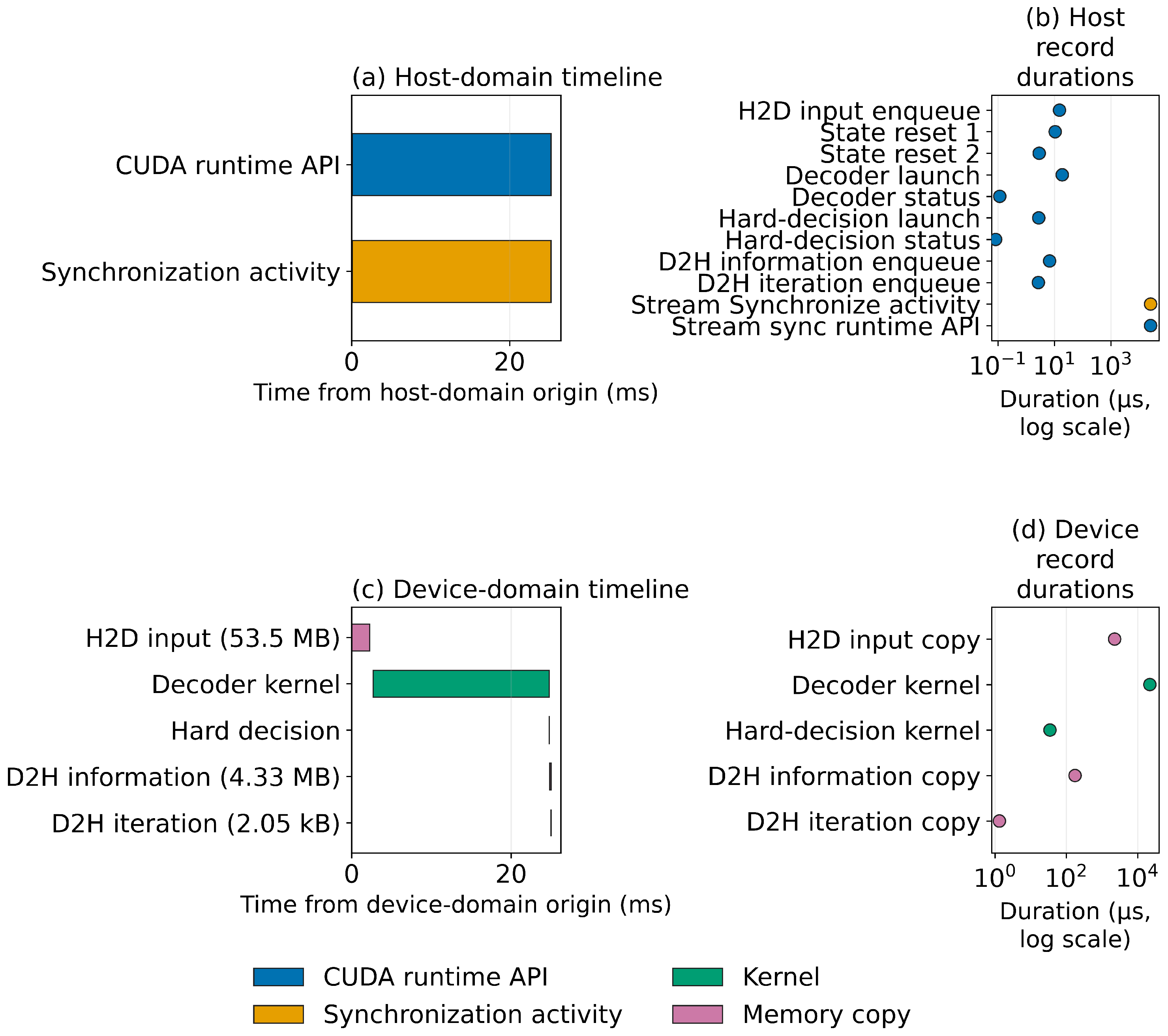
CUPTI recovered correlated records with no dropped activities in 3600 traced layered trials. At batch 512 under the layered full boundary, P50/P99 durations were 24.951/26.235 ms for the inclusive runtime API, 24.881/26.168 ms for the overlapping synchronization call, 21.894/23.218 ms for summed kernels, and 2.423/2.514 ms for summed memory copies. The records locate activity within the diagnostic execution, but their overlapping intervals and separate host/device origins prevent an additive decomposition. Figure A2 and Figure A3 in Appendix C provide the complete diagnostic views. Fixed-clock control and privileged counters remained unavailable, so driver delay, PCIe contention, memory stalls, and active-SM execution cannot be separated causally.
5. Discussion
5.1. Interpretation of Schedule and Repeated-Session Results
The flooding implementation required more time at P50 and P99 in every same-cap cell. Its kernel makes three lifted-edge traversals per iteration rather than two, maintains old and new message buffers, and uses a different reset path. These implementation differences are consistent with the observed ordering, although the experiment does not estimate their individual contributions. The matched outcome study adds an important qualification: among words that satisfied the syndrome under both schedules by the tested cap, the layered implementation had a lower conditional first-satisfaction iteration in every estimable 2- and 4-dB cell. This comparison is cap-dependent and does not include words censored by failure to satisfy the syndrome. Both schedules used the same prespecified ; schedule-specific parameter tuning could alter the convergence comparison. The result therefore compares these implementations and settings, not intrinsically optimal versions of the two schedules.
The batch-64-to-128 result was not invariant to experimental design. The baseline scaling and component-timing designs produced large contractions, whereas the schedule/boundary design and all six replication sessions produced positive layered full-boundary estimates. The positive session-specific direction persisted under the resampling sensitivities and leave-one-session-out summaries, but six sessions do not support population-level coverage. Moreover, separately seeded batches do not estimate the effect of appending codewords to a fixed input set, and the executable and allocation footprint differ between the two design groups. The evidence therefore establishes design sensitivity, not the reason for it. The theoretical 264-block resource ceiling cannot explain either direction without an achieved-residency measurement.
For layered decoding, endpoint levels differed across the separately acquired full, decode-only, and transfer-only boundaries. The comparison documents boundary-specific distributions, not additive transfer or non-decoder contributions. In instrumented runs, upper host-latency observations were associated with longer within-SM block durations; in separate traced runs, CUPTI located overlapping API, kernel, memory-copy, and synchronization intervals. Neither diagnostic maps additively to the unprofiled tail sample or distinguishes driver scheduling, dynamic clocks, memory behavior, PCIe contention, or active execution. Preheating changed several variables together, and its two narrowly positive full-boundary intervals were not stable across all resampling schemes.
5.2. Practical Meaning of the Metrics
expresses the absolute separation between P50 and P99, whereas is the P99-to-P50 ratio; the median-relative separation is . Equation (7) shows why their empirical directions can differ when the median changes. They are two interpretations of the same quantiles rather than independent outcomes. P99 remains the latency endpoint; neither derived metric defines a budget or supports interpolation between the tested batches.
The full-boundary measurement is synchronous decoder-batch completion, not per-codeword or receiver latency. A batch of B codewords is submitted as one decoder-kernel grid with B CUDA blocks, one per codeword; the reported time ends when the entire batch completes. A physical-layer budget would also include CRC processing and hybrid automatic repeat request (HARQ) control:
Percentiles of dependent stages cannot generally be added to obtain the percentile of their sum. The measured P99 values therefore characterize one decoder term in Equation (9), not full-PHY, radio-interface, application, or URLLC latency.
At 2 and 4 dB, early stopping reduced latency when it reduced the iteration count, but rose because P50 fell proportionally faster. At 0 dB, it saved no iterations, added 20 syndrome sweeps, and moved P50 and P99 in opposite directions at batch 16. Evaluation therefore depends on channel condition, iteration cap, batch size, and syndrome-check schedule.
5.3. Limitations and Future Work
All measurements use one consumer GPU under dynamically clocked WSL2. Six separately initiated acquisition sessions provide repeated measurements within this installation but do not substitute for operating-system restarts, native Linux, or independent device replication. No intentionally competing GPU workload was launched, but the experiment did not establish exclusive control of host, desktop, driver, or virtualization activity. With only six sessions, the two-stage bootstrap is a descriptive stability analysis rather than a calibrated population inference. Unavailable fixed clocks and privileged counters leave achieved occupancy, active warps, cache and memory traffic, per-trial PCIe use, and virtualization effects unresolved.
The benchmark excludes rate recovery, traffic arrivals, multi-stream overlap, other physical-layer kernels, and application integration. FP32 is a validation reference. Across the graph and schedule studies, only three graph/lifting configurations, one implemented rate per base graph, and three channel conditions were tested. The schedules share one normalization value rather than separately optimized parameters, and the experiment does not factor schedule from every implementation choice or establish equal optimization maturity. The all-zero and random input modes use separate codeword and noise seeds, so that control compares distributions rather than matched-noise payload effects; codeword symmetry does not remove this timing-design limitation. Within each timing visit, 200 repetitions reuse one input batch; they measure execution variability but are not 200 independent channel realizations. The block bootstrap resamples 100 visit blocks per primary cell and 40 per replication session, so its intervals remain conditional on those blocks and the dependence model. P99.9 and maxima are finite-sample descriptions, not worst-case bounds.
The next platform experiments should test native Linux, a second GPU architecture, and fixed clocks with performance-counter access. Counter-enabled profiling should measure achieved occupancy, active warps, cache and memory traffic, and per-trial PCIe activity. Reduced-precision comparisons should evaluate FP16 and INT8 at matched information-bit BER and information-word BLER. Multi-stream studies should report transfer–computation overlap, and fuller-receiver studies should include rate recovery. Matched CPU and FPGA comparisons require the same code configuration, precision, stopping rule, error target, and timing boundary.
6. Conclusions
GPU LDPC latency comparisons depend on decoder schedule, batch granularity, convergence behavior, and timing boundary. We used a boundary-explicit empirical framework that combined P50, P99, , , paired-block resampling, matched decoding outcomes, three timing boundaries, and session replication. Flooding had higher P50 and P99 in 15 same-cap cells, although and had no uniform ordering. At batch 512 and 20 iterations, flooding exceeded layered decoding by 12.812 ms at P50 and 13.102 ms at P99. At 2 dB and cap 20, the mean first-satisfaction iteration among the 20,000 matched words satisfying the syndrome under both schedules was 5.78 for layered decoding and 9.64 for flooding. At batch 512, layered decode-only P50 and P99 were 2.925 and 3.265 ms below the separately acquired full-boundary endpoints; these differences are not additive component estimates. Across six sessions, full-boundary increased by s from batch 64 to 128 (pointwise descriptive 95% interval, –s), whereas the baseline scaling and component-timing designs produced decreases. Together, these findings show that schedule, decoding-outcome context, timing boundary, and acquisition design must be reported together. They apply to the tested FP32 implementations with on one dynamically clocked GPU under WSL2 and do not establish microarchitectural causation, worst-case or cross-platform behavior, or URLLC compliance.
Author Contributions
Conceptualization, S.J. and E.K.; methodology, S.J.; software, S.J.; validation, S.J. and E.K.; formal analysis, S.J.; investigation, S.J.; resources, S.J.; data curation, S.J.; writing—original draft preparation, S.J.; writing—review and editing, S.J. and E.K.; visualization, S.J.; supervision, E.K.; project administration, E.K. All authors have read and agreed to the published version of the manuscript.
Funding
This research received no external funding.
Institutional Review Board Statement
Not applicable.
Informed Consent Statement
Not applicable.
Data Availability Statement
The source code and baseline timing dataset are publicly available at https://github.com/pz1004/5G-NR-BG1-LDPC-Decoding (accessed on 10 September 2026). The additional raw datasets supporting the algorithmic-control, schedule, timing-boundary, operating-state, and diagnostic analyses are available from the corresponding author upon reasonable request.
Acknowledgments
The authors acknowledge the use of OpenAI Codex as described in Materials and Methods. The authors retain full responsibility for the content of the publication.
Conflicts of Interest
The authors declare no conflicts of interest.
Appendix A. Detailed Comparison Matrices
The following tables provide the complete schedule, outcome, boundary, component, and operating-state matrices summarized in the main text. They are derived from the experimental observations described in Methods and Appendix C.
Appendix A.1. Literature Comparison Matrices
Table A1.
Configuration and algorithm fields reported for cited GPU LDPC operating points. Length and rate follow each source’s convention. N/R means not reported; no missing value is inferred.
Table A2.
Stopping, precision, and software fields reported for the same GPU LDPC operating points. N/R means not reported; no missing value is inferred.
Table A3.
Reported execution granularity, performance, software, and timing boundaries for the same operating points. Latency and throughput values may come from different points within a source and are not ranked against this work. DTP: data-transfer process.
Table A4.
Reported execution granularity, performance, software, and timing boundaries (continued). Values may come from different operating points within a source and are not ranked against this work. DTP: data-transfer process.
Appendix A.2. Experimental and Statistical Matrices
Table A5.
Zero-observed-error cross-cap timing contrasts: flooding at cap 20 minus layered at cap 10, at 2 dB. Pointwise 95% percentile intervals use 5000 paired circular moving-block replicates over acquisition blocks (). The zero observed bit and information-word errors and full final-syndrome success come from separate, untimed, non-batch-stratified 20,000-word outcome cells; the latency contrasts come from the listed timing-batch cells with separately generated inputs. This overlay is not a joint equal-performance or equivalence analysis.
Table A6.
Acquisition-specific batch-64-to-128 evidence. Pointwise 95% percentile intervals use 5000 paired circular moving-block replicates over acquisition blocks (). Acquisitions are displayed separately and are not pooled or meta-analyzed.
Table A7.
Session-specific batch-64-to-128 differences in s. Entries are estimates with pointwise 95% percentile intervals from 5000 paired circular moving-block bootstrap replicates over the 40 ordered blocks in each session ().
Table A8.
Preheated-minus-idle-cooled endpoint contrasts and the full-minus-decode difference-in-differences at batch 512. Entries are estimates with pointwise 95% percentile intervals from 5000 paired circular moving-block bootstrap replicates over 30 ordered cycles ().
Table A9.
Schedule latency endpoints. Pointwise 95% percentile intervals use 5000 paired circular moving-block replicates with the acquisition block as the resampling unit and ordered circular runs of length ; they are descriptive and not multiplicity-adjusted.
Table A10.
Schedule paired endpoint contrasts (right minus left). Pointwise 95% percentile intervals use 5000 paired circular moving-block replicates with the acquisition block as the resampling unit and ordered circular runs of length ; they are descriptive and not multiplicity-adjusted.
Table A11.
Paired random-valid-codeword decoding outcomes for the layered and flooding implementations. Each 20,000-word cell was decoded in chunks of at most 256 words (78 full chunks and one 32-word chunk). “Final syndrome” tests the decoder output after the stated fixed cap; “ever satisfied” records whether the syndrome was satisfied at least once by that cap. Because fixed decoding continues after a first success, these indicators can differ. Under an independent and identically distributed word-level Bernoulli model, parenthetical limits are one-sided 95% exact Clopper–Pearson bounds for a zero event rate or, when the observed event rate is one, for the zero complementary-failure rate. Zero BER denotes no observed information-bit errors; no independent-bit confidence bound is claimed. First-satisfied-iteration summaries are conditional on ever-satisfied words. These word-level results are not organized as acquisition blocks and do not use the acquisition-block bootstrap.
Table A12.
Paired schedule outcome contrasts (flooding minus layered). Pointwise 95% percentile intervals use 5000 paired ordinary bootstrap replicates of matched words; they are descriptive and not multiplicity-adjusted. A binary contrast with no discordant paired-word outcomes is marked N/E because an empirical bootstrap point mass at zero does not quantify population uncertainty. First-iteration differences and the empirical flooding/layered convergence ratio are conditional on ever satisfying the syndrome under both schedules. The ratio is specific to each tested SNR/cap cell and is not an iteration-equivalence factor. This word-level bootstrap is separate from the ordered-block latency bootstrap.
Table A13.
Boundary latency endpoints. Pointwise 95% percentile intervals use 5000 paired circular moving-block replicates with the acquisition block as the resampling unit and ordered circular runs of length ; they are descriptive and not multiplicity-adjusted.
Table A14.
Boundary paired endpoint contrasts (right minus left). Pointwise 95% percentile intervals use 5000 paired circular moving-block replicates with the acquisition block as the resampling unit and ordered circular runs of length ; they are descriptive and not multiplicity-adjusted.
Table A15.
Boundary-study component medians. The synchronized host total uses the host steady clock. The raw components, signed remainder, and event-zero-to-event-five total use the CUDA-event clock, which was not cross-calibrated to host elapsed time. Observation by observation, the five named raw components plus the signed remainder equal the separately queried total by construction; this is an arithmetic within-stream identity check, not evidence of an independent decomposition. Separately computed medians need not obey the observation-level identity.
Table A16.
Component P99 values for the tested batch-512, 20-iteration cells. Panel A uses the synchronized host steady-clock domain; Panel B gives raw CUDA-event-clock values that were not cross-calibrated to host elapsed time. Values across panels are not compared or combined. The CUDA total is separately queried using the same event-zero and event-five endpoint events; the signed remainder is that total minus the five named component intervals. This arithmetic within-stream identity check does not constitute independent decomposition evidence.
Table A17.
Observation-level timer consistency for the five batch-512, 20-iteration dynamic-clock cells. The synchronization ratios and host-total-minus-wait P99 values use paired host-clock observations. The host-shorter count and host-minus-CUDA mean test cross-domain enclosure; because that check failed, the CUDA-event values are not treated as calibrated to host elapsed time. These diagnostics are not an additive timing decomposition.
Table A18.
Six-session stability summary for the batch-64-to-128 contrasts under the schedule-generalized benchmark. The estimand is the equal-weight mean of the six session-specific contrasts, not a pooled-observation quantile contrast. Intervals are pointwise descriptive 95% percentile intervals from a two-stage bootstrap that resamples sessions and then paired ordered blocks within the selected session (5000 replicates; inner primary ); they are neither calibrated population-coverage intervals nor multiplicity-adjusted tests.
Table A19.
Operating-state resampling sensitivity. Direction labels compare the primary paired circular moving-block result at with , , and paired independent whole-cycle resampling. Each method uses 5000 replicates and pointwise descriptive 95% percentile intervals; no interval is multiplicity-adjusted.
Table A20.
Timer-consistency diagnostics for selected session-replication cells. Synchronization fractions and host-total-minus-wait values use paired host-clock observations. Host-shorter counts test enclosure across distinct clock domains; failure of that check precludes treating the raw CUDA-event values as calibrated to host elapsed time. Ranges span the listed cells or sessions.
Table A21.
Operating ranges from continuous 100-ms telemetry. Statistics use samples with a valid metric-specific status; valid and total sample counts are stated in each panel heading.
Table A22.
Descriptive Spearman associations between block-level latency summaries and operating-condition summaries for the baseline and algorithmic-control layered BG1 , 20-iteration acquisitions. Each row contains 100 acquisition blocks. Baseline telemetry comprises one before/after pair per complete block; algorithmic-control telemetry uses visit-level samples. Temperature, clocks, power, utilization, and order covary, so these coefficients neither isolate a causal effect nor provide a fixed-clock comparison. N/E denotes a coefficient that is not estimable because memory clock was constant.
Table A23.
NVML clock-event counts among valid samples. The GPU-idle bit is informational rather than a thermal or power-throttling event. Every other documented bit—application clock setting, software power cap, hardware slowdown, synchronized boost, software or hardware thermal slowdown, power brake, and display clock setting—was zero in both studies.
Appendix B. Algorithmic and Configuration Sensitivity
The following tables and Figure A1 report the complete workload, algorithm, convergence, stopping, channel, input, graph, and lifting-size controls summarized in the main text.
Table A24.
Primary BG1, end-to-end batch-latency results. Panel A reports observation accounting. Pointwise 95% percentile intervals in Panels B and C use 5000 paired circular moving-block bootstrap replicates over ordered acquisition blocks (); they are descriptive and not multiplicity-adjusted. Ten planned warm-ups preceded retention at every visit; no retained observation was excluded after acquisition.
Table A25.
Finite-sample primary tail descriptions in s from 20,000 retained observations per cell; no retained observation was excluded. P99.9 and the observed maximum have no bootstrap intervals and are not used to classify configuration contrasts or as worst-case bounds.
Figure A1.
BG1 scaling endpoints at batches 4, 16, 64, 128, 192, 256, 320, and 512 and fixed iteration counts 5, 10, and 20. Error bars are pointwise descriptive 95% percentile intervals from 5000 paired circular moving-block bootstrap replicates over ordered acquisition blocks (L = 5); they are not multiplicity-adjusted. The categorical horizontal axis displays every tested batch.
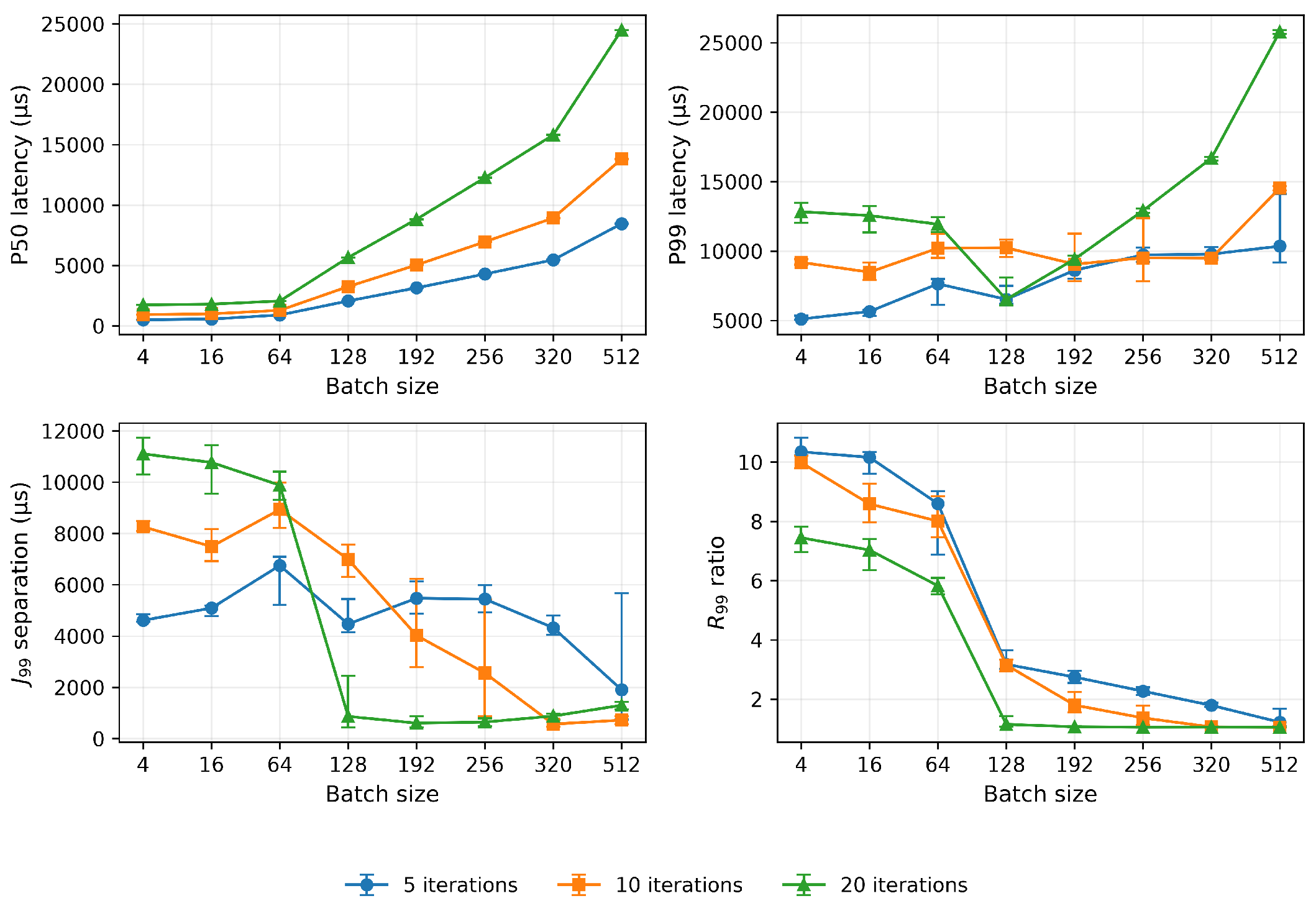
Table A26.
Algorithm sensitivity at 20 fixed iterations, dB, and BG1 . Panel A reports algorithm parameters and observation counts. Pointwise 95% percentile intervals in Panels B and C use 5000 paired circular moving-block bootstrap replicates over ordered acquisition blocks (); they are descriptive and not multiplicity-adjusted. Each cell has zero post-acquisition exclusions.
Table A27.
Untimed error and convergence study for 20,000 random valid BG1 codewords per cell with a 20-iteration cap. Panel A reports information-bit BER, information-word BLER, and syndrome-success rate. Panel B reports first-satisfied-iteration summaries conditional on words that satisfied the syndrome within the cap; NA denotes no successful word. The OMS 0-dB convergence summaries are conditional on one successful word.
Table A28.
Channel, input, and stopping-policy sensitivity (20-iteration cap, BG1 ). Panel A reports the configuration and mean executed iterations. Pointwise 95% percentile intervals in Panels B–D use 5000 paired circular moving-block bootstrap replicates over ordered acquisition blocks (); they are descriptive and not multiplicity-adjusted. Random-minus-all-zero contrasts are reported separately.
Table A29.
Random-minus-all-zero input contrasts. Panel A reports mean executed-iteration differences. Pointwise 95% percentile intervals in Panels B and C use 5000 paired circular moving-block bootstrap replicates over ordered acquisition blocks (); they are descriptive and not multiplicity-adjusted. Mean-iteration differences are point estimates.
Table A30.
Finite-sample 0-dB tail diagnostics. Panel A reports executed iterations, P97.5, and P99. Every observation reached the 20-iteration cap. P97.5 is descriptive and is not an additional primary endpoint. Panel B reports the upper tail quantiles and the probability of exceeding the fixed-cap P99.
Table A31.
Base-graph and lifting-size controls at 20 fixed iterations. Panel A reports location and tail quantiles. Pointwise 95% percentile intervals use 5000 paired circular moving-block bootstrap replicates over ordered acquisition blocks (); they are descriptive and not multiplicity-adjusted. Panel B reports the corresponding and separation measures.
Appendix C. Measurement Validation and Supplementary Methods
The scientific samples comprise 1,840,000 algorithmic-control timings, 600,000 schedule timings, 300,000 boundary timings, 384,000 session-replication timings, 24,000 operating-state timings, and 72,000 block-placement timings. The matched outcome analysis contains 360,000 decoded rows representing 60,000 unique codeword/noise pairs. No timing observation was excluded because of its magnitude. CUPTI supplied a separate diagnostic sample of 3600 traced trials with no dropped activity records.
The operating-state sample contains 30 complete cycles. In one additional cycle, a sampled software-power-cap event appeared after the preheated visits and before the idle-cooled visits. That incomplete cycle contains 400 timing records, 500 untimed preconditioning executions, and 4856 telemetry samples; none enters the primary analysis. Table A19 reports analyses that omit the corresponding complete cycle or substitute the available preheated records. The 41,000 preconditioning executions reported for the primary dataset are the total across its 30 complete cycles.
The two matched outcome acquisitions used identical codeword/noise pairs and produced identical decoded outcomes and convergence records for every word. One acquisition is analyzed, and the second establishes deterministic repeatability; they are not pooled. Their latency and visit-level telemetry are not used for inference because the experiment was designed as an untimed outcome comparison.
Four timer sources appear in the supplementary analyses: the host monotonic clock, same-stream CUDA events, %globaltimer, and CUPTI activity timestamps. The WSL2 host/CUDA enclosure check failed, and cross-SM %globaltimer comparability was not established. Cross-domain differences and cross-SM spans are therefore not interpreted as physical components. Fixed application clocks, achieved occupancy, active-warps measurements, privileged DRAM/L2 traffic counters, and per-trial PCIe attribution were unavailable. CUPTI supplied runtime, synchronization, kernel, and memory-copy intervals but no performance counters.
Figure A2.
Mean inferred maximum overlapping blocks per SM in the instrumented layered-decoder diagnostic. Values use within-SM %globaltimer comparisons only. Cross-SM timing was not validated, and the trace changed P50; the figure is not an achieved-occupancy or device-wide concurrency measurement.
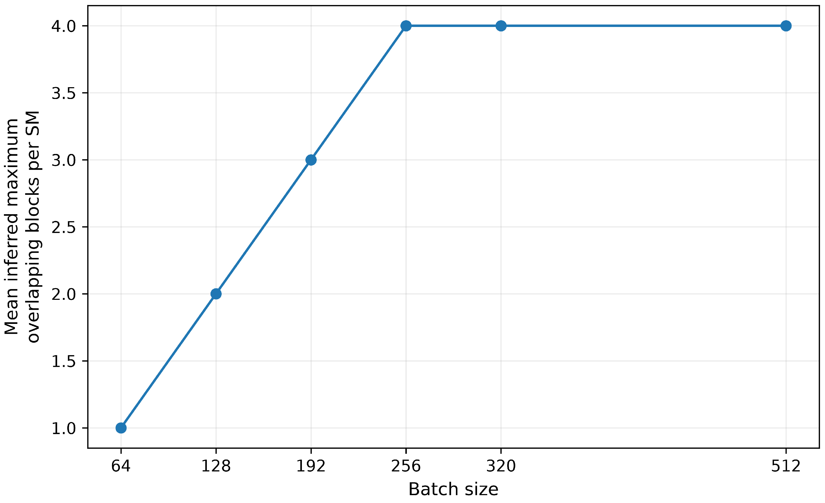
Figure A3.
CUPTI Activity records for the first retained traced trial of invocation 1 at batch 512 under the layered full boundary (external correlation identifier 901). Panels (a,c) show the host- and device-domain timelines, respectively, using independent timestamp origins. Panels (b,d) report the duration of every corresponding record on logarithmic axes. Blue, orange, green, and purple identify CUDA runtime API, synchronization activity, kernel, and memory-copy records; lane and operation labels provide the same distinctions without reliance on color. The cudaStreamSynchronize runtime-API interval and the stream-synchronization activity interval cover the same blocking period and must not be added. CUPTI-traced trials are excluded from the unprofiled latency sample.
References
- 5G Americas. New Services & Applications with 5G Ultra-Reliable Low Latency Communications; Technical Report; 5G Americas: Bellevue, WA, USA, 2018; Available online: https://www.5gamericas.org/new-services-applications-with-5g-ultra-reliable-low-latency-communications/ (accessed on 27 July 2026).
- Liang, B.; Gregory, M.A.; Li, S. Latency Analysis for Mobile Cellular Network uRLLC Services. J. Telecommun. Digit. Econ. 2022, 10, 39–57. [Google Scholar] [CrossRef] [Scilit]
- Gallager, R.G. Low-Density Parity-Check Codes. IRE Trans. Inf. Theory 1962, 8, 21–28. [Google Scholar] [CrossRef] [Scilit]
- 3rd Generation Partnership Project (3GPP). NR; Multiplexing and Channel Coding. 3GPP Technical Specification 38.212, European Telecommunications Standards Institute, 2026. Release 18; ETSI TS 138 212 V18.8.0. Available online: https://www.etsi.org/deliver/etsi_ts/138200_138299/138212/18.08.00_60/ts_138212v180800p.pdf (accessed on 27 July 2026).
- Aronov, A.; Kazakevich, L.; Mack, J.; Schreider, F.; Newton, S. 5G NR LDPC Decoding Performance Comparison Between GPU & FPGA Platforms. In Proceedings of the 2019 IEEE Long Island Systems, Applications and Technology Conference (LISAT); IEEE: New York, NY, USA, 2019; pp. 1–6. [Google Scholar] [CrossRef] [Scilit]
- Li, R.; Zhou, X.; Pan, H.; Su, H.; Dou, Y. A High-Throughput LDPC Decoder Based on GPUs for 5G New Radio. In Proceedings of the 2020 IEEE Symposium on Computers and Communications (ISCC); IEEE: New York, NY, USA, 2020; pp. 1–7. [Google Scholar] [CrossRef] [Scilit]
- Ling, J.; Cautereels, P. Fast LDPC GPU Decoder for Cloud RAN. IEEE Embed. Syst. Lett. 2021, 13, 170–173. [Google Scholar] [CrossRef] [Scilit]
- Tarver, C.; Tonnemacher, M.; Chen, H.; Zhang, J.; Cavallaro, J.R. GPU-Based, LDPC Decoding for 5G and Beyond. IEEE Open J. Circuits Syst. 2021, 2, 278–290. [Google Scholar] [CrossRef] [Scilit]
- Dai, J.; Yin, H.; Lv, Y.; Xu, W.; Yang, Z. Multi-Gbps LDPC Decoder on GPU Devices. Electronics 2022, 11, 3447. [Google Scholar] [CrossRef] [Scilit]
- Liu, Z.; Zhao, L. High-Throughput Software LDPC Decoder on GPU. EURASIP J. Adv. Signal Process. 2024, 2024, 91. [Google Scholar] [CrossRef] [Scilit]
- Qi, Z.; Yao, Y.; Li, Y.; Tung, C.H.; Zheng, J.; Zhuo, D.; Chen, T. DecodeX: Exploring and Benchmarking of LDPC Decoding across CPU, GPU, and ASIC Platforms. In HotMobile ’26: Proceedings of the 27th International Workshop on Mobile Computing Systems and Applications, Atlanta, GA, USA, 25–26 February 2026; Association for Computing Machinery: New York, NY, USA, 2026; pp. 127–132. [Google Scholar] [CrossRef] [Scilit]
- Kato, S.; Lakshmanan, K.; Rajkumar, R.; Ishikawa, Y. TimeGraph: GPU Scheduling for Real-Time Multi-Tasking Environments. In Proceedings of the 2011 USENIX Annual Technical Conference (USENIX ATC 11), Portland, OR, USA, 15–17 June 2011; pp. 17–30. Available online: https://www.usenix.org/conference/usenixatc11/timegraph-gpu-scheduling-real-time-multi-tasking-environments (accessed on 29 August 2026).
- Elliott, G.A.; Ward, B.C.; Anderson, J.H. GPUSync: A Framework for Real-Time GPU Management. In Proceedings of the 2013 IEEE 34th Real-Time Systems Symposium, IEEE Computer Society, Vancouver, BC, Canada, 3–6 December 2013; IEEE: New York, NY, USA, 2013; pp. 33–44. [Google Scholar] [CrossRef] [Scilit]
- Gheibi-Fetrat, A.; Safari, S.; Hessabi, S.; Sarbazi-Azad, H. RTGPU: Real-Time Computing with Graphics Processing Units: Architectures, Challenges, and Solutions for Time-Critical GPU Systems; Synthesis Lectures on Computer Architecture; Springer Nature: Cham, Switzerland, 2026. [Google Scholar] [CrossRef] [Scilit]
- Richardson, T.J.; Shokrollahi, M.A.; Urbanke, R.L. Design of Capacity-Approaching Irregular Low-Density Parity-Check Codes. IEEE Trans. Inf. Theory 2001, 47, 619–637. [Google Scholar] [CrossRef] [Scilit]
- Chen, J.; Dholakia, A.; Eleftheriou, E.; Fossorier, M.P.C.; Hu, X.Y. Reduced-Complexity Decoding of LDPC Codes. IEEE Trans. Commun. 2005, 53, 1288–1299. [Google Scholar] [CrossRef] [Scilit]
- Hocevar, D.E. A Reduced Complexity Decoder Architecture via Layered Decoding of LDPC Codes. In Proceedings of the IEEE Workshop on Signal Processing Systems (SIPS), Austin, TX, USA; IEEE: New York, NY, USA, 2004; pp. 107–112. [Google Scholar] [CrossRef] [Scilit]
- Kelkar, A.; Dick, C. NVIDIA Aerial GPU Hosted AI-on-5G. In Proceedings of the 2021 IEEE 4th 5G World Forum (5GWF); IEEE: New York, NY, USA, 2021; pp. 64–69. [Google Scholar] [CrossRef] [Scilit]
- Notari, E.F.; Travassos, X.L. 5G New Radio Open Radio Access Network Implementation in Brazil: Review and Cost Assessment. Telecom 2025, 6, 24. [Google Scholar] [CrossRef] [Scilit]
- Arabian, F.; Shoushtari, M. A Comparative Study of Waveforms Across Mobile Cellular Generations: From 0G to 6G and Beyond. Telecom 2025, 6, 67. [Google Scholar] [CrossRef] [Scilit]
- Lin, X.; Kundu, L.; Cammerer, S.; Huang, Y.; Dick, C.; Santhosam, C.; Gadiyar, R.; Wiesmayr, R.; Studer, C. AI-Native 6G: Empowering Intelligent RAN with Accelerated Compute. IEEE Wirel. Commun. 2025, 32, 11–14. [Google Scholar] [CrossRef] [Scilit]
- Coles, S. An Introduction to Statistical Modeling of Extreme Values; Springer Series in Statistics; Springer: London, UK, 2001. [Google Scholar] [CrossRef] [Scilit]
- Künsch, H.R. The Jackknife and the Bootstrap for General Stationary Observations. Ann. Stat. 1989, 17, 1217–1241. [Google Scholar] [CrossRef] [Scilit]
- Politis, D.N.; Romano, J.P. A Circular Block-Resampling Procedure for Stationary Data. In Exploring the Limits of Bootstrap; LePage, R., Billard, L., Eds.; Wiley Series in Probability and Mathematical Statistics; John Wiley & Sons: New York, NY, USA, 1992; pp. 263–270. [Google Scholar]
- Lahiri, S.N. Resampling Methods for Dependent Data; Springer Series in Statistics; Springer: New York, NY, USA, 2003. [Google Scholar] [CrossRef] [Scilit]
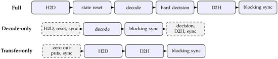
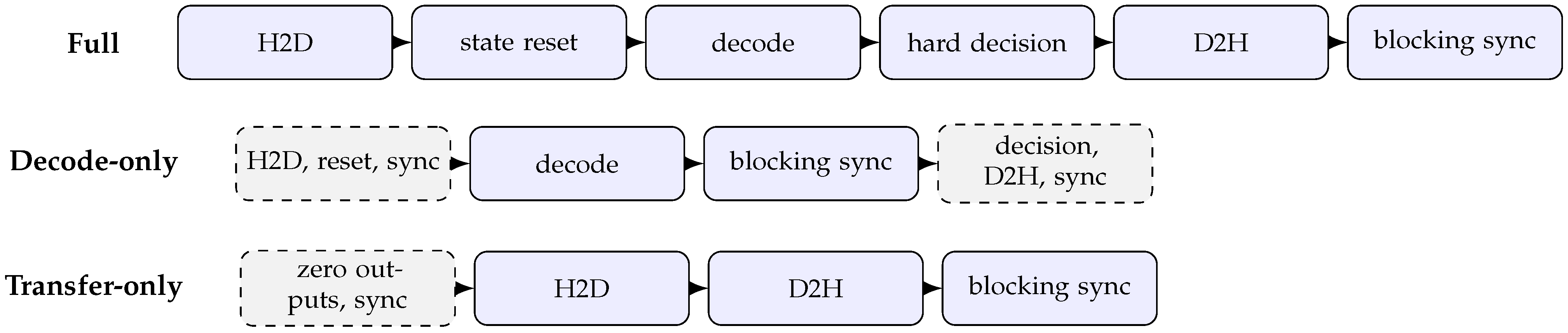
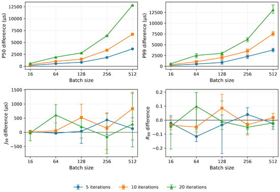
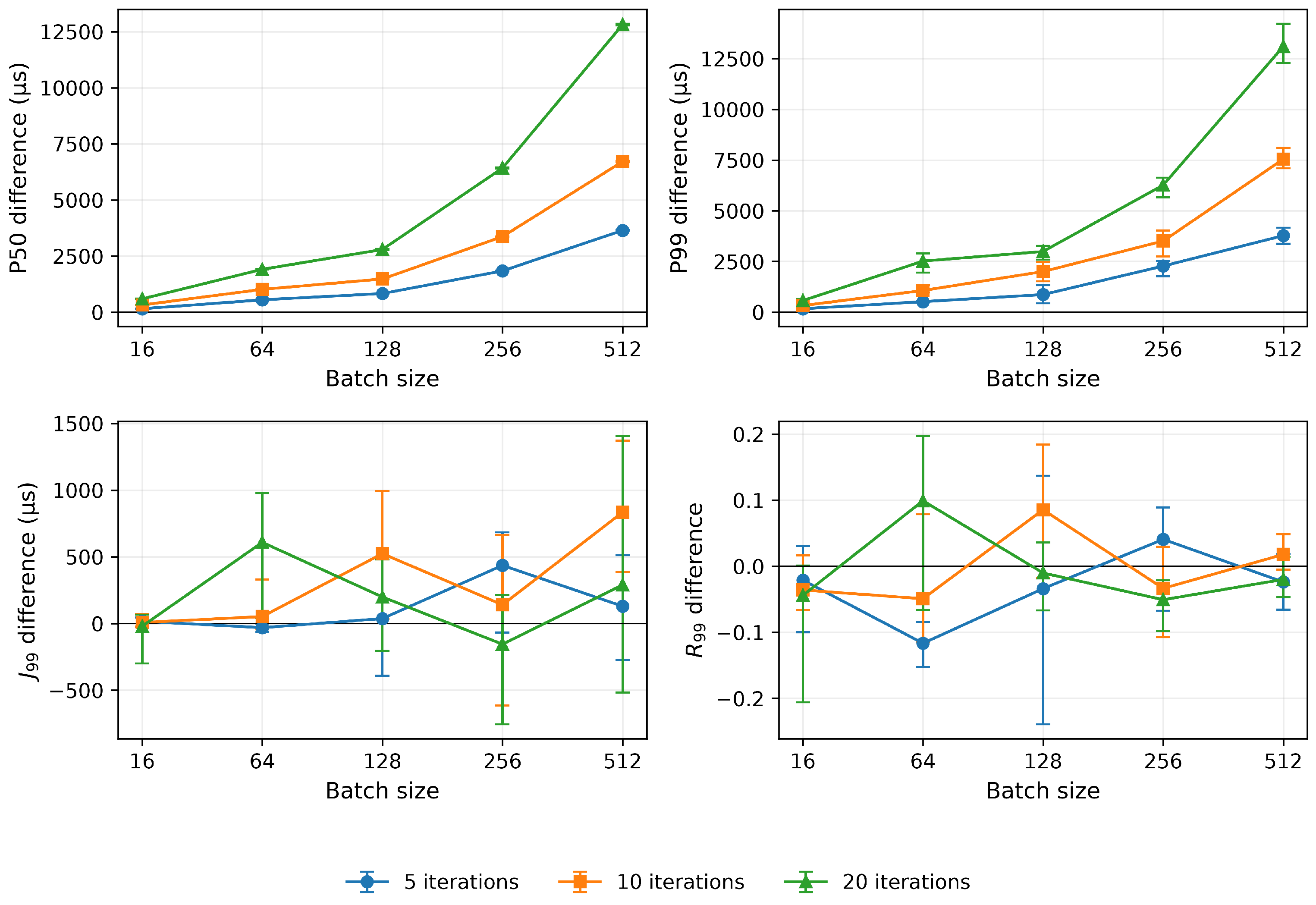
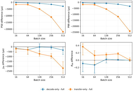
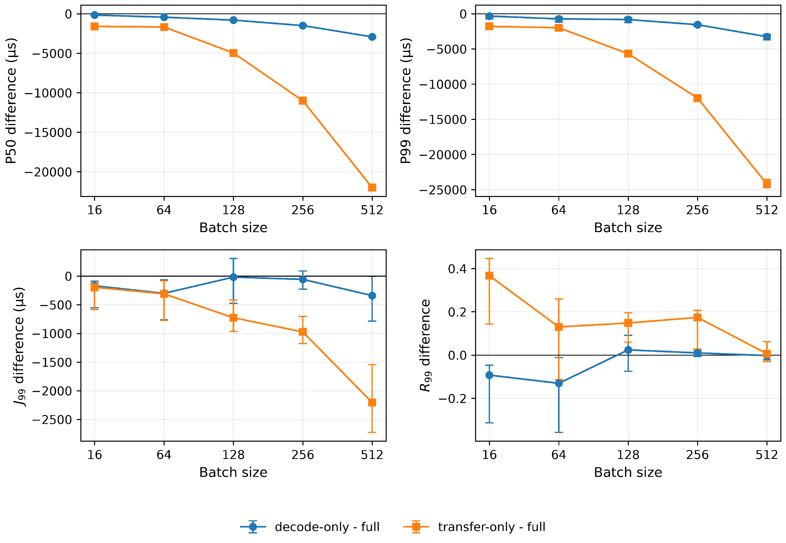
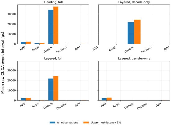
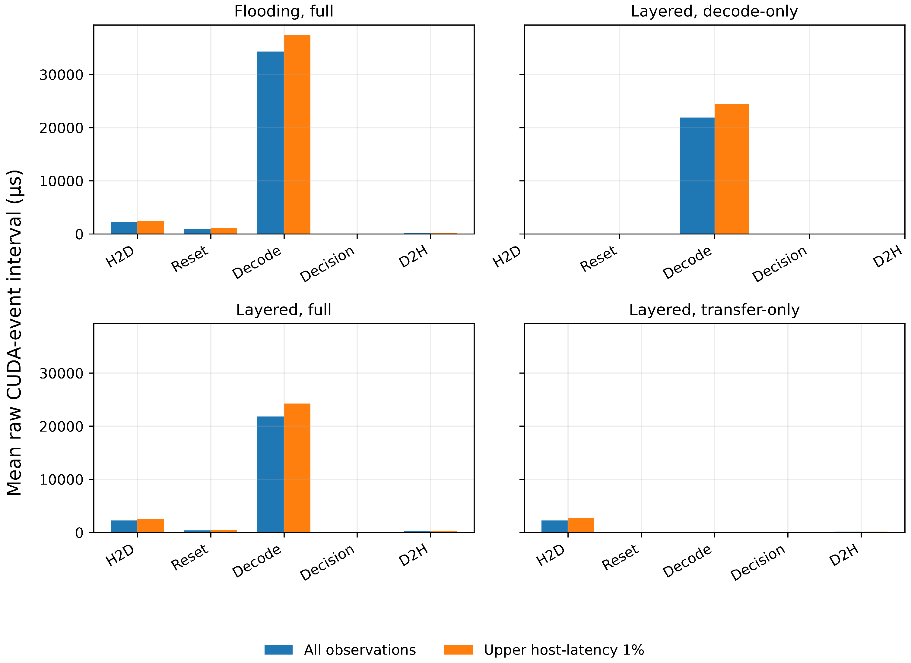
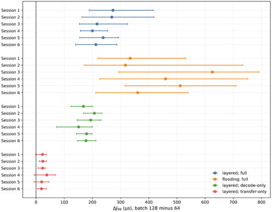
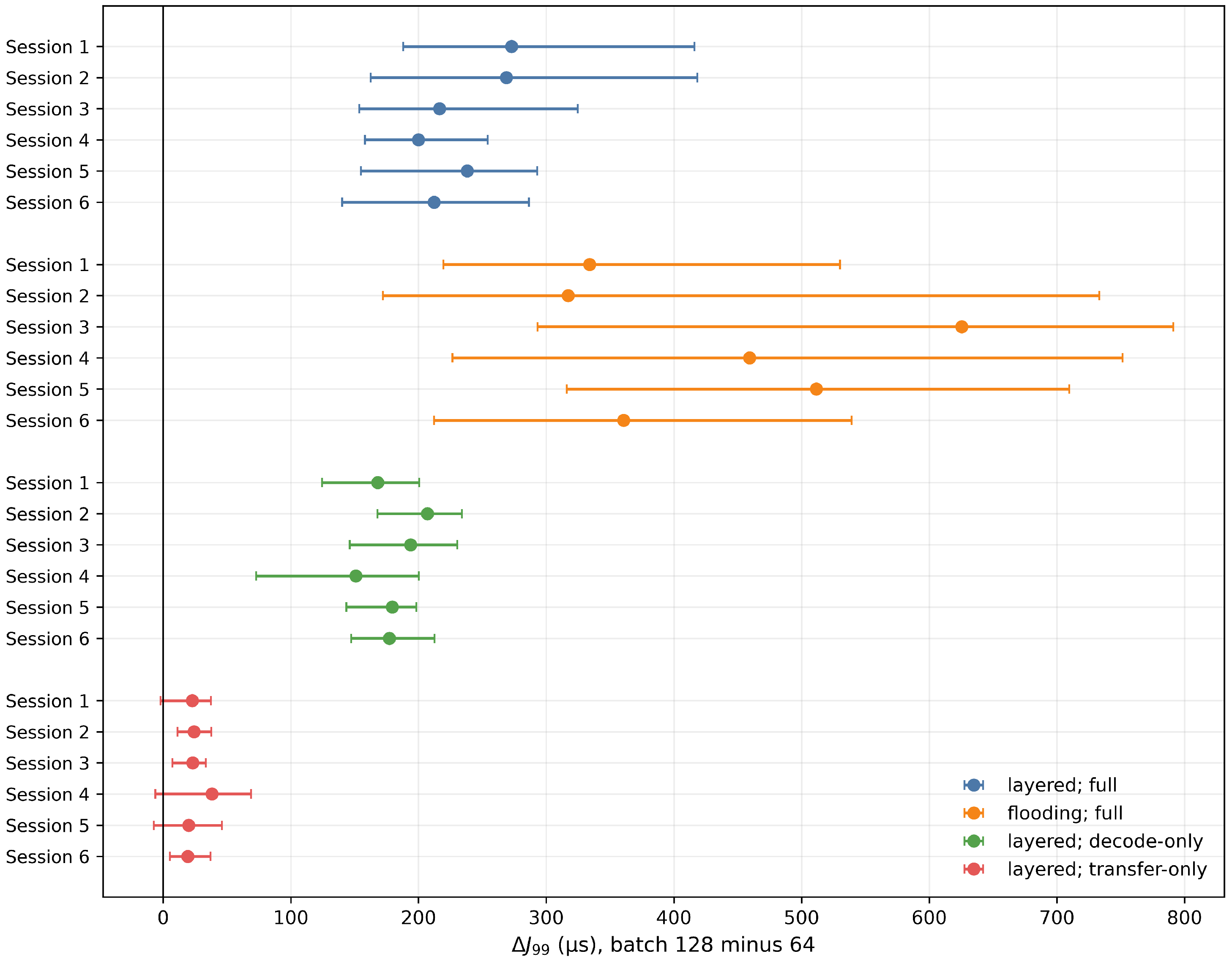
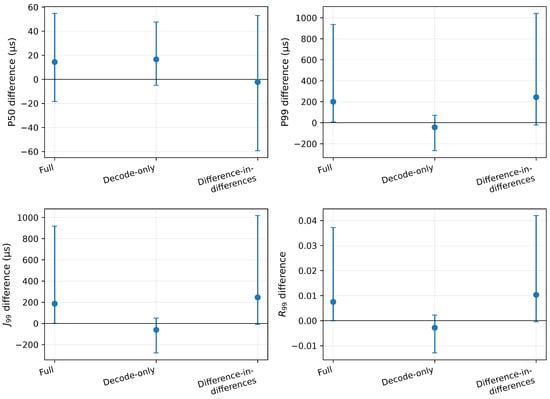
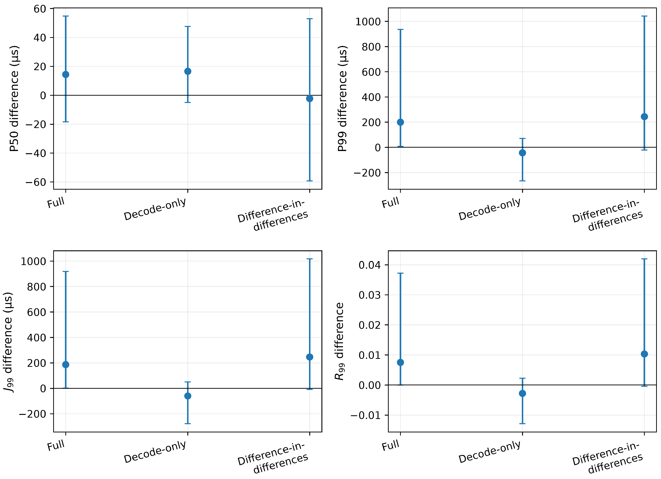

Disclaimer/Publisher’s Note: The statements, opinions and data contained in all publications are solely those of the individual author(s) and contributor(s) and not of MDPI and/or the editor(s). MDPI and/or the editor(s) disclaim responsibility for any injury to people or property resulting from any ideas, methods, instructions or products referred to in the content. |
© 2026 by the authors. Licensee MDPI, Basel, Switzerland. This article is an open access article distributed under the terms and conditions of the Creative Commons Attribution (CC BY) license.