


Abstract
Reliable dynamic spectrum access in wide-area cognitive radio networks (CRNs) is challenged by sparse and erroneous spectrum-sensing measurements. This work formulates spatial-spectrum occupancy reconstruction as an image inpainting problem and proposes two cascaded deep learning models: a bidirectional long short-term memory-based image inpainting model (BiLSTM-IIM) and a binary diffusion-based image inpainting model (Diff-IIM). In both models, Stage 1 corrects sensing errors at observed locations, while Stage 2 reconstructs missing entries. The models are evaluated using simulations of a cognitive radio network with 50–200 secondary users, five primary users, and three spatial resolutions under representative wireless conditions. Both models generally outperform total variation and matrix completion baselines under sparse and noisy observations. Under moderate sensing errors, BiLSTM-IIM achieves accuracies of 92.91%, 93.66%, and 91.17% at the , , and resolutions, respectively, while Diff-IIM achieves lower false-alarm rates with fewer parameters. Stage 1 reduces the sensing-error rate by approximately 58% for BiLSTM-IIM and 61% for Diff-IIM. These results support deep learning-based inpainting for wide-area spectrum occupancy reconstruction under the evaluated conditions.
1. Introduction
Efficient spectrum utilization has become a pressing issue due to the rapid growth of wireless devices and services. Cognitive radio networks (CRNs) have emerged as a promising paradigm to improve spectrum availability by enabling secondary users (SUs) to opportunistically access licensed frequency bands without interfering with primary users (PUs) [1,2].
CRNs utilize a dynamic spectrum access framework which relies critically on accurate spectrum occupancy prediction to ensure reliable operation and efficient resource allocation [3,4]. However, spectrum prediction remains highly challenging, particularly in wide-area deployments where measurements are sparse and inaccurate. The vast geographical scale of CRNs, coupled with temporal variability in spectrum usage and the prohibitive cost of continuous sensing, and hardware limitations of sensing devices, leads to incomplete occupancy estimates [5,6,7]. Sparse observations result in missed opportunities, increased interference risks, and degraded quality of service. Hence, the precise detection of spectrum band occupancy is vital for cognitive radio (CR) functionality since it underpins all secondary transmission strategies [8].
To address this challenge, we reformulate spectrum prediction as an image inpainting problem [5]. With this formulation, the frequency bands are represented as image channels and spatial locations as pixels. Incomplete spectrum maps are treated as images with missing pixels, and the task becomes reconstructing missing occupancy information [9,10]. Since spectrum sensing in wide-area cognitive radio networks [11,12] is generally sparse, incomplete and noisy [13,14,15,16], this formulation enables CRNs to benefit from advances in image-based inpainting methods. In addition, this image representation enables the prediction model to exploit both spatial correlations across neighboring locations and spectral correlations across licensed frequency bands [17,18].
In this work, two deep learning models are explored: a Bidirectional Long Short-Term Memory-based image inpainting model (BiLSTM-IIM) and a Binary Diffusion-based image inpainting model (Diff-IIM). The BiLSTM-IIM is suitable because it learns contextual dependencies in flattened spatial-spectrum representations from both forward and backward directions [19,20]. Also, the Diff-IIM is suitable because spectrum occupancy is binary in nature, corresponding to idle or occupied states [6]. By using a bit-flip diffusion process, the model preserves the discrete structure of the spectrum occupancy map while learning to reconstruct missing binary occupancy values from sparse observations [21,22].
Although prior studies have investigated spectrum prediction using statistical, machine learning, and deep learning techniques, most existing methods formulate the problem as temporal forecasting, regression, or channel-state prediction at selected locations. In contrast, the reconstruction of a complete wide-area spatial-spectrum occupancy map from sparse measurements remains less explored. Our prior work demonstrated the feasibility of spectrum inpainting using Total Variation minimization [5]; however, optimization-based inpainting methods may struggle under highly sparse sensing conditions. This motivates the use of learning-based image inpainting models that can exploit spatial and spectral dependencies learned from historical data for more accurate spectrum occupancy reconstruction.
The novelty of this work lies in extending spectrum occupancy prediction from conventional temporal forecasting or regression-based formulations to a deep learning-based image inpainting framework for wide-area spectrum map reconstruction [2,6,19,23,24,25]. Unlike traditional spectrum prediction approaches that mainly estimate channel states at selected locations or time instances, the proposed approach reconstructs a complete spatial-spectrum occupancy map from sparse measurements. Compared with prior Total Variation-based spectrum inpainting [5] and Matrix Completion (MC) [26] baselines, this work introduces and evaluates two learning-based inpainting models, BiLSTM-IIM and Diff-IIM, which are capable of learning complex spatial and spectral dependencies from data [21,24]. Furthermore, this work provides insight into the effects of sensing errors, sparsity and spatial resolution on spectrum occupancy reconstruction.
We make the following contributions:
- Image inpainting-based formulation: We formulate spectrum occupancy prediction in cognitive radio networks as an image inpainting problem, where spatial locations are treated as pixels and frequency channels as image channels. This enables complete spectrum maps to be reconstructed from sparse and imperfect secondary-user observations.
- Cascaded deep learning models for noisy observations: We develop and evaluate two-stage learning-based image inpainting models: BiLSTM-IIM and Diff-IIM. In both models, Stage 1 refines noisy known observations caused by sensing false alarms and missed detections, while Stage 2 completes the missing entries.
- Analysis of sparsity, resolution, and sensing errors: We analyze reconstruction performance across different grid resolutions (, , and ), different numbers of SUs, and multiple sensing-error scenarios. This allows the effects of observation density, spatial resolution, and sensing reliability to be jointly evaluated.
- Stage 1 error correction ablation: We verify the role of the Stage 1 correction module by comparing the original incomplete observations with the Stage 1 corrected outputs at known locations.
The remainder of this paper is organized as follows. Section 2 reviews related work on spectrum occupancy prediction, image inpainting techniques, and deep learning applications in cognitive radio networks. Section 3 presents the system model, data generation procedure, and formulation of the spectrum occupancy reconstruction problem. Section 4 describes the proposed image inpainting-based methodology, including BiLSTM-IIM, Diff-IIM, and the Total Variation (TV) and Matrix Completion (MC) baselines. Section 5 details the experimental setup, including the datasets, model training, model configurations, and evaluation metrics. Section 6 presents and discusses the experimental results, including dataset characteristics, reconstruction performance, sensing-error analysis, and ablation studies. Finally, Section 7 concludes the paper and outlines directions for future work.
2. Related Work
Research on spectrum occupancy prediction has evolved from early statistical modeling techniques to advanced deep learning approaches [19]. While image inpainting techniques [9] have proven effective for reconstructing missing data in image processing applications, their application to wireless networks remains largely unexplored, with the notable exception of our previous work [5]. The rapid adoption of deep learning in cognitive radio networks has opened promising avenues for achieving reliable spectrum prediction under sparse sensing conditions. In the following subsections, we review prior studies across three key areas: spectrum occupancy prediction methods, image inpainting techniques, and deep learning applications in CRNs. This review highlights the limitations of existing approaches and establishes the motivation for our proposed method.
2.1. Spectrum Occupancy Prediction
Accurate spectrum occupancy prediction is essential in cognitive radio networks (CRNs), as it enables secondary users (SUs) to opportunistically access available channels while avoiding unwanted interference with primary users [27]. Early approaches relied on statistical and signal processing models such as hidden Markov models [28,29], autoregressive models [30,31], and Kalman filtering [32]. These methods provided useful temporal forecasts but were limited in their ability to generalize under practical network conditions.
More recently, machine learning and deep learning approaches have been introduced, including support vector machines, decision trees, convolutional neural network (CNN)-based models, long short-term memory (LSTM)-based models, hybrid LSTM-multilayer perceptron (MLP) models, graph neural networks, and Transformer-based architectures [14,23,24,25,33,34,35]. These approaches have improved spectrum prediction accuracy by learning nonlinear temporal, spectral, and spatial correlations in spectrum usage data. Recent studies have also explored advanced deep learning frameworks, such as 3D vision Transformer-based spectrum prediction, to capture the evolution of spectrum usage patterns across time, frequency, and space [14]. In addition, spectrum cartography and radio-map completion studies have investigated the reconstruction of spectrum or radio maps from limited measurements using matrix completion and learned neural models [16,18,33]. However, most existing spectrum prediction studies still focus primarily on temporal forecasting, channel-state prediction, or radio-map estimation, rather than reconstructing a complete binary spatial-spectrum occupancy map from sparse secondary-user observations. This distinction motivates the proposed image inpainting-based formulation.
2.2. Image Inpainting Techniques
Image inpainting is the task of reconstructing missing or corrupted regions of an image by making use of information from other surrounding pixels. Early inpainting techniques were optimization-based, including total variation minimization. These methods are effective for smooth areas but tend to oversmooth structures and lose detail when large portions of data are missing.
With the rise of machine learning, data-driven methods such as sparse coding, dictionary learning, and more recently, convolutional neural networks [36] have been applied to inpainting. Modern advances include generative adversarial networks [37] and diffusion models [38,39], which learn high-level structural priors from data and produce realistic reconstructions even under severe corruption. These approaches have proven far more effective than traditional optimization methods in preserving texture and global structure.
The connection of image inpainting to spectrum occupancy prediction emerges when spectrum sensing maps are treated as images. Missing or incomplete measurements correspond to corrupted pixels, and the goal becomes reconstructing the complete occupancy map, similar to a prior work that converted power spectrum map estimation into an image reconstruction task [40].
In our previous work [5], spectrum prediction was formulated as an image recovery problem and solved using Total Variation (TV) inpainting. This demonstrated the feasibility of treating sparse spectrum sensing as an image reconstruction problem. However, TV inpainting is an optimization-based method and may degrade under highly sparse observations. Matrix completion is another classical optimization-based reconstruction approach for recovering missing entries from incomplete observations [26]. It assumes that the unknown complete matrix has an underlying low-rank structure, so the missing entries can be inferred from correlations among the observed entries. However, this assumption may be limited for sparse, binary, and noisy spectrum occupancy maps with heterogeneous PU coverage and sensing errors.
These limitations motivate the use of learning-based reconstruction methods, namely BiLSTM-IIM and Diff-IIM, which are designed to learn spatial and spectral dependencies from data and improve reconstruction accuracy under sparse and noisy sensing conditions.
3. Problem Formulation and Data Generation
The spectrum occupancy prediction problem we aim to solve in this work is shown in Figure 1. We formulate the problem as an image inpainting task, and the goal is to reconstruct missing or unobserved spectrum occupancy based on a partially known and noisy spectrum pattern or map. In our formulation, SUs act as distributed spectrum sensors, and their local observations are aggregated into a sparse grid, with ten frequency channels. In the spectrum maps, red indicates PU-occupied regions, green shows detected idle areas, and gray represents unknown status due to partial sensing. The incomplete, spatial–spectral map is fed into a deep learning model, which predicts the full spectrum occupancy.
Figure 1.
Spectrum occupancy prediction problem formulated as an image inpainting task: from partial sensing to complete spectrum reconstruction.
3.1. Network Area Discretization and Image Mapping
The network area considered in this work spans . Five primary users are randomly placed within the region, while the number of secondary users varies from 50 to 200 in increments of 10. To evaluate the effect of spatial granularity on spectrum occupancy reconstruction, the continuous network area is discretized into three spatial grid resolutions: , , and .
For a given grid, the corresponding spatial step sizes are defined as
Thus, the , , and grids correspond to spatial step sizes of , , and , respectively.
After the spatial step size is determined, each user located at continuous spatial coordinates is mapped to a discrete grid location using the rounding operation:
The resulting values are then clipped to remain within the valid grid range:
where and are the final clipped grid indices.
The resulting discrete grid can be expressed as an image of size , where each grid cell corresponds to one pixel in the image domain. Lower resolutions, such as , reduce computational cost and provide higher observation density for a fixed number of secondary users. Higher resolutions, of , provide finer spatial granularity but increase sparsity and computational costs. In this study, all three grid resolutions are considered to evaluate their impact on spectrum occupancy reconstruction.
3.2. Simulation of Complete Spectrum Occupancy
The complete spectrum occupancy dataset was generated using a realistic cognitive radio simulation framework motivated by prior studies on cognitive radio networks [41,42], spectrum sensing [43,44], primary-user activity modeling [45], wireless propagation [46,47], radio environment maps [48], and sparse spectrum reconstruction [49]. The simulation incorporates heterogeneous primary-user coverage, shadowing-based irregular propagation, random PU activity, contiguous channel occupation, clustered secondary-user deployment, probabilistic sensing, multi-channel sensing, and imperfect sensing. All of these are considered to better reflect practical cognitive radio sensing conditions and to generate incomplete spectrum observations that are both sparse and noisy.
Following the discretization procedure in Section 3.1, the complete spectrum occupancy map is generated separately for , , and grid resolutions. For each grid resolution, the number of licensed channels is . Since this work focuses on one-shot spectrum occupancy reconstruction, each input sample corresponds to a single spectrum snapshot rather than a temporal prediction sequence. Therefore, for a given grid, the complete spectrum occupancy map is represented as
where , and . For each grid location and channel, c, denotes a truly idle channel, while denotes a truly occupied channel. The binary occupancy representation is used as a decision-level abstraction of spectrum availability. This directly follows from the objective of this work: to predict whether each spatial-channel entry is idle or occupied for dynamic spectrum access, and not to estimate raw RF signal power or waveform-level measurements.
Five primary users are deployed in the network area. To model heterogeneous PU coverage, each PU is assigned an interference radius
This allows different PUs to have different interference radius that shows variation in transmit power, antenna characteristics, and propagation conditions. In addition, to model propagation variability and avoid perfectly circular coverage regions, a spatially varying shadowing factor is introduced as
so that the effective coverage radius of PU p at grid location becomes
The heterogeneous PU radii represent variations in transmit power and propagation range, while the spatially varying variable changes the effective coverage boundaries to represent large-scale spatial propagation variability caused by terrain, obstructions, scattering, and shadow fading [47,49]. Accordingly, the spatial effects of path loss and shadowing in practical wireless propagation are incorporated in the simulation through variations in the effective PU coverage boundaries rather than through a received-power model [50]. Figure 2 compares ideal circular PU coverage with the heterogeneous, shadowing-based PU coverage adopted in the simulation.
Figure 2.
Illustration of heterogeneous and shadowing-based PU coverage. The left panel shows idealized circular PU coverage with fixed interference radius. The right panel shows the realistic PU coverage model used in this work. The heterogeneous interference radii and spatially varying shadowing indicate irregular coverage boundaries.
For each generated spectrum snapshot, each PU p is assigned an activity state , where represents an inactive PU and represents an active PU. The activity state is generated according to the PU activity model used in the simulation. When a PU is active, it occupies a contiguous block of licensed channels. The number of occupied channels is selected as
and the starting channel is randomly chosen such that the occupied block remains within the available channels. A PU-to-PU channel-conflict check is also applied to prevent nearby PUs with overlapping interference regions from being assigned the same channel.
The complete occupancy map is generated by marking a grid location as occupied if it lies within the effective coverage region of at least one active PU using the corresponding channel. Formally, if there exists at least one PU p such that
where is the set of channels occupied by PU p, is the distance between grid location and PU p in pixel units, and is the resolution-dependent spatial step size. Otherwise, . For each active PU, all possible contiguous channel blocks are first generated and randomly shuffled. Each candidate block is then compared with the channel blocks already assigned to previously processed active PUs. Let denote the distance between PU p and a previously assigned PU q in pixel units. The two PUs are considered nearby if
If two nearby PUs share at least one channel, the candidate channel block is rejected. Otherwise, the candidate block is assigned to PU p. If no valid channel block is available after checking all candidates, PU p is treated as inactive for that snapshot.
The complete spectrum occupancy map for one spectrum snapshot is generated using Algorithm 1. In this work, , , and . The same procedure is repeated independently to generate the dataset for each grid resolution.
3.3. Simulation of Incomplete Spectrum Occupancy
The incomplete spectrum observation map is generated to model the real-world sparse and imperfect information available to the CRNs. In practical deployments, SUs are generally nonuniformly distributed over a wide area [51]. They may concentrate around buildings, roads, campuses, residential areas, or other high-traffic hotspots, resulting in uneven observation density where some regions are either well sensed or poorly observed [51]. In addition, SUs may not sense or report at every sensing instant due to battery limitations, mobility, hardware limitations, or temporary communication failure [51,52]. Practical SUs may also have different sensing capabilities, where some devices sense only one channel while others scan multiple channels using wider bandwidth, faster sensing hardware, or longer sensing duration [43]. Furthermore, spectrum sensing decisions are not always correct in real environments because noise, fading, shadowing, receiver limitations, and low signal-to-noise ratio can cause missed detections and false alarms [53,54]. Therefore, the incomplete observation map is generated using clustered SU deployment, probabilistic SU reporting, multi-channel sensing, and imperfect sensing decisions.
| Algorithm 1 Simulation of complete spectrum occupancy map. |
| Require:
Grid size , channels C, PUs P, network size Ensure: Complete occupancy map
|
3.3.1. Secondary-User Deployment
Let denote the number of secondary users. In this study, the number of SUs varies from 50 to 200 in increments of 10:
To model nonuniform sensing density, SUs are deployed using a clustered spatial distribution. Let denote the number of SU clusters. In this work,
The cluster centers are generated randomly within the network region. Each SU is placed around one of the cluster centers with probability
while the remaining SUs are placed uniformly across the network area with probability
For a clustered SU, the location is generated by adding a Gaussian perturbation around the selected cluster center:
where
and the cluster spread is set to
This clustered deployment produces nonuniform sensing density across the network, such that some regions are densely observed while others remain sparsely observed. After generating the continuous spatial locations of SUs, each location is then mapped to the discrete grid using the mapping procedure described in Section 3.1.
3.3.2. Intermittent SU Participation
To model intermittent sensing and reporting, each SU senses and reports with probability
Thus, the sensing participation variable for SU s is modeled as
where indicates that SU s senses and reports, and indicates that SU s does not contribute an observation.
This probabilistic reporting captures the fact that not all SUs are available or able to report during every sensing instant.
3.3.3. Multi-Channel SU Sensing
If SU s participates in sensing, it observes multiple licensed channels. The number of sensed channels is selected as
where denotes the discrete uniform distribution. The selected channel set is then drawn without replacement from the licensed channels, such that
This models heterogeneous SU sensing capability, where different SUs may contribute different amounts of spectral information.
3.3.4. Incomplete Observation Map
For each considered grid resolution, the incomplete observation map has the same spatial and spectral dimensions as the complete occupancy map and is denoted as
where , and . The observation states are defined as
Here, i and j denote the spatial grid location, and c denotes the licensed channel index. All entries of Y are initially set to the unknown state:
3.3.5. Imperfect Sensing Model
When SU s senses channel at its grid location , the observation is generated from the true state using an imperfect sensing model. The missed detection probability and false alarm probability are set according to the level of error:
A missed detection occurs when an occupied channel is incorrectly sensed as idle, while a false alarm occurs when an idle channel is incorrectly sensed as occupied. Therefore, the conditional sensing probabilities are
and
Under a moderate-error condition, unoccupied and idle channels are correctly detected with probability , respectively. These probabilities introduce a potential uncertainty in the sensing system, since the observation reported by an SU may differ from the true channel state. At the level of sensing, the false alarm probability and misdetection probability represent the effects of receiver noise, fading, shadowing, receiver limitations, and low signal-to-noise ratio on the simulated binary occupancy states. The error-level scenarios (error-free, moderate-error and high-error) represent increasing levels of sensing difficulties.
Thus, the generated incomplete observation map is not only sparse due to limited SU sensing but also noisy due to sensing errors, making the reconstruction task more representative of practical cognitive radio sensing conditions.
For each participating SU s and each sensed channel, , the incomplete observation map is updated as
where is the imperfect sensing outcome generated according to the conditional probabilities above. All unsensed entries remain unknown. The incomplete spectrum observation map for one spectrum snapshot is generated using Algorithm 2. The same procedure is repeated independently for each complete occupancy map, SU-density setting, and grid resolution.
3.3.6. Learning Objective
The final learning task is to reconstruct the complete occupancy map X from the incomplete and imperfect observation map Y:
where represents the proposed image inpainting-based reconstruction model. This formulation allows the proposed model to learn from incomplete spatial-spectral observations and infer the missing spectrum occupancy states across locations and channels.
| Algorithm 2 Simulation of incomplete spectrum occupancy map. |
| Require:
Complete map , SUs , channels C Ensure: Incomplete map
|
4. Methodology
This section presents four approaches adopted in this study for spectrum occupancy image inpainting: two proposed deep-learning models, namely (i) a Bidirectional Long Short-Term Memory-based image inpainting model (BiLSTM-IIM) and (ii) a diffusion-based image inpainting model based on the Binary Diffusion Model (Diff-IIM) in [21]; and two classical baselines, namely (iii) Total Variation image inpainting baseline (TV-IIM) and (iv) matrix completion image inpainting model (MC-IIM). The deep-learning models were selected and adapted to match the spatial, multi-channels, and binary properties of the spectrum occupancy maps. These properties differ from those of natural images, which generally contain continuous pixel values and are usually reconstructed to preserve visual appearance. While BiLSTM-IIM exploits spatial encoding using convolution, and bidirectional cross-channel modeling, Diff-IIM utilizes bit-flip diffusion that is consistent with the binary nature of the spectrum maps. These methods adopt a two-stage approach: Stage 1 corrects errors due to false measurements at observed locations, and Stage 2 focuses on reconstruction of missing entries using the corrected measurements. Together, these design choices address sensing errors and missing observations as distinct reconstruction tasks to achieve reliable complete-map reconstruction from sparse and noisy measurements.
4.1. BiLSTM-Based Image Inpainting Model (BiLSTM-IIM)
The proposed BiLSTM-based image inpainting model (BiLSTM-IIM) is implemented as a two-stage mask-guided CNN-BiLSTM architecture specifically designed for spectrum occupancy image inpainting. While CNNs [55], LSTMs/BiLSTMs [56], and masking strategies in image inpainting [57] are established components, their integration in the proposed two-stage reconstruction framework is tailored to reconstruct complete spectrum occupancy maps from sparse and noisy secondary-user observations. In this architecture, a lightweight convolutional encoder extracts local spatial features from each licensed-channel map, while the BiLSTM component models inter-channel dependencies across the licensed channels. This design enables the model to exploit both spatial structures within each channel and spectral correlations across frequency bands.
For a given incomplete observation map, Y, defined in (22), entries with the unknown label 2 are first remapped to to explicitly represent missing observations in the model input. Two binary masks are then constructed: a known-location mask and a missing-location mask , where
and
A zero-filled observation map is then constructed from Y by replacing the missing entries with 0. Since 0 is also a valid idle-state value, is not used alone. Instead, it is concatenated with and , allowing the model to distinguish truly observed idle locations from missing locations that were filled with zero for numerical input.
The proposed BiLSTM-IIM is trained in two cascaded stages. In Stage 1, the model receives three input maps for each licensed channel—the filled observation map, the known-location mask, and the missing-location mask:
Each licensed-channel input is processed independently by a lightweight two-dimensional CNN encoder. The encoder consists of a standard convolutional layer, batch normalization, ReLU activation, a depthwise convolutional layer, a pointwise convolutional layer, adaptive average pooling, and a linear projection. The CNN produces one embedding vector for each licensed channel. Therefore, for a sample with C channels, the CNN encoder converts the channel-wise input maps into a sequence of C feature vectors:
where is the CNN embedding dimension.
The resulting channel-feature sequence is passed to a bidirectional LSTM with one recurrent layer and 128 hidden units in each direction. Since the sequence length corresponds to the number of licensed channels, the BiLSTM models dependencies across the channel embeddings rather than treating the full spatial map as a long flattened sequence. The output corresponding to each channel is then passed through layer normalization, dropout, and a fully connected prediction head to produce the Stage-1 logits.
The Stage-1 objective is summarized as
where BCE is binary cross-entropy, denotes the Stage-1 CNN-BiLSTM model, is the Stage-1 logit output, and X is the complete ground-truth occupancy map. The term denotes the binary cross-entropy loss computed only over the known locations indicated by . Thus, Stage 1 is trained to correct noisy observed entries while excluding unknown locations from the loss computation.
The Stage-1 logits are converted to probabilities using the sigmoid function:
where denotes the sigmoid function. The probability map is then thresholded to obtain the binary Stage-1 prediction:
where denotes the indicator function and is the decision threshold.
A Stage-1 cleaned incomplete map is then formed by combining the thresholded Stage-1 prediction with the original mask information:
where ⊙ denotes element-wise multiplication. In this expression, is used to replace the observed known locations with the Stage-1 corrected binary values, while the missing locations remain encoded as .
In Stage 2, the trained Stage-1 model is frozen, and its output is used to guide the missing-location completion stage. Stage 2 receives the mask-guided input:
and the reconstruction objective is summarized as:
Here, denotes the Stage-2 CNN-BiLSTM model, is the Stage-2 reconstruction, and and denote the masked binary cross-entropy losses computed over missing and known locations, respectively. In this work, and are used to emphasize missing-location reconstruction while retaining a smaller known-location term for consistency after Stage 1 correction.
During inference, the final cascaded reconstruction is obtained by using the Stage-1 output at known locations and the Stage-2 output at missing locations:
where ⊙ denotes element-wise multiplication. The sigmoid-activated outputs are thresholded at 0.5 to obtain the final binary occupancy predictions. Figure 3 summarizes the two-stage mask-guided reconstruction flow of the proposed BiLSTM-IIM.
Figure 3.
Two-stage mask-guided reconstruction flow of the proposed BiLSTM-IIM. The incomplete observation map is first converted into a filled observation map and two masks indicating observed and missing locations. Stage 1 corrects noisy observed entries using a known-location masked loss and produces a cleaned incomplete map. Stage 2 uses the same masks together with the Stage-1 outputs to complete missing locations. The final reconstruction is obtained by combining the Stage-1 prediction at observed locations with the Stage-2 prediction at missing locations.
4.2. Diffusion-Based Image Inpainting Model (Diff-IIM)
The proposed Diffusion-Based Image Inpainting Model (Diff-IIM) also follows a two-stage cascaded binary diffusion framework, which employs a binary bit-flipping diffusion formulation that is suitable for the binary composition of the spectrum occupancy map, unlike Gaussian diffusion models which inject continuous-valued noise.
Let denote the complete ground-truth occupancy map and let denote the incomplete observation map, where represents an unknown entry. The known-location and missing-location masks, and , are defined in (30) and (31), respectively, and are reused in Diff-IIM to indicate observed and missing entries.
In addition, two observation-indicator maps are constructed as
Here, identifies observed idle entries and identifies observed occupied entries. These indicator maps allow the model to distinguish observed idle locations from missing locations.
4.2.1. Binary Forward Diffusion
During training, a timestep t is sampled uniformly from , where in this work. The bit-flip probability is generated using a quadratic schedule:
where , and . Given the clean binary map X, the corrupted diffusion state is generated as
where ⊕ denotes bitwise XOR. Thus, each binary occupancy value is flipped with probability .
4.2.2. Stage 1: Known-Location Error Correction
For each sample, the Stage-1 input is formed by concatenating the noisy diffusion state , the observed-idle indicator , the observed-occupied indicator , and the missing-location mask :
Since each component has C channels, the Stage-1 input has channels. This stage network is trained to produce logits:
where denotes the Stage-1 time-conditioned diffusion network. The Stage-1 loss is computed using binary cross-entropy with logits over the known locations only:
Here, denotes binary cross-entropy with logits between the Stage-1 logits and the ground-truth map X, computed only over entries selected by . This objective trains Stage 1 to correct noisy observed entries while excluding unknown locations from the loss computation.
After Stage 1 is trained, it is used as a frozen correction module. The Stage-1 logits are passed through a sigmoid function and thresholded to obtain a binary prediction:
Only the known-location part of this prediction is retained:
The corresponding cleaned incomplete map is expressed as
Thus, Stage 1 corrects the observed locations while keeping missing locations encoded as unknown.
4.2.3. Stage 2: Missing-Location Completion
Stage 2 uses the frozen Stage-1 corrected known map to reconstruct the missing locations. During training, a noisy binary diffusion state is generated from the clean ground-truth map using the same bit-flipping process in (43). The Stage-2 input is
The Stage-2 network produces logits
where denotes the Stage-2 time-conditioned diffusion network, trained using a missing-location masked BCE-with-logits loss:
Here, denotes the binary cross-entropy with logits between the Stage-2 logits and the ground-truth map X, computed only over the missing entries indicated by . This objective focuses Stage 2 on completing the unknown entries, while the Stage-1 corrected known map.
4.2.4. Lightweight Time-Conditioned Denoising Network
Figure 4 illustrates the lightweight time-conditioned denoising CNN used in the proposed Diff-IIM framework. The network receives a stage-specific input tensor formed by channel-wise concatenation of the noisy map and the corresponding auxiliary information. For Stage 1, the input is given by (44), while for Stage 2, the input is given by (50).
Figure 4.
Architecture of the lightweight time-conditioned denoising CNN used in the proposed Diff-IIM framework. The network processes a stage-specific input tensor using two residual encoder blocks, an SE attention block, and two decoder blocks. The diffusion timestep is encoded using a sinusoidal embedding and projected through an MLP before being concatenated with the encoded feature map. The final convolution produces the 10-channel occupancy logits.
The input tensor is first processed by two residual encoder blocks. The first encoder block maps the stage-specific input channels to 128 feature channels, while the second encoder block expands the representation from 128 to 256 channels. An SE attention block is then applied to recalibrate the 256-channel feature representation before decoding. In parallel, the diffusion timestep t is encoded using a 16-dimensional sinusoidal time embedding and projected through a multilayer perceptron (MLP) to obtain a 128-dimensional time-conditioning feature. This time feature is spatially expanded and concatenated with the 256-channel encoded feature map, producing a 384-channel input to the first decoder block.
The first decoder block reduces the feature dimension from 384 to 128 channels, followed by a dropout layer with probability . The second decoder block further reduces the representation from 128 to 64 channels. Finally, a convolution maps the 64-channel feature representation to the C-channel output logits, where is the number of spectrum channels. The output logits are converted to binary occupancy estimates using a sigmoid activation followed by a fixed threshold of .
4.2.5. Cascaded Inference
During inference, Stage 1 first produces the corrected known-location map . Stage 2 is then initialized by preserving the Stage 1 corrected known entries and randomly initializing the missing entries:
At each reverse step, the Stage 2 denoising network predicts logits , which are converted to a binary proposal using a sigmoid activation followed by a fixed threshold:
The reverse update preserves the Stage 1 corrected known entries and updates only the missing locations:
After the final reverse step, the reconstructed occupancy map is obtained as
This cascaded inference procedure allows Stage 1 to correct noisy observed measurements and Stage 2 to complete the missing spectrum occupancy entries.
4.3. Baseline: Total Variation Image Inpainting
We adopt the Total Variation (TV) inpainting method as a baseline for complete spectrum map recovery. TV is selected as a benchmark because it has been widely recognized in the literature as an effective tool for image restoration [58,59,60] by enforcing piecewise smooth reconstructions.
Given an incomplete spectrum occupancy map, Y, and a known-location mask, , TV-IIM reconstructs the complete map by solving
where promotes piecewise smoothness, and the data-consistency term preserves the observed known entries.
4.4. Baseline: Matrix Completion
We also include Matrix Completion (MC) as an additional classical optimization-based reconstruction baseline. Matrix Completion, hereafter referred to as Matrix Completion Image Inpainting Model (MC-IIM), is selected as a baseline because it is a widely used optimization-based method for recovering missing entries from incomplete data [26].
Given an incomplete spectrum occupancy map, Y, and a known-location mask, , the spatial-spectrum tensor is reshaped into a matrix, and the missing entries are estimated by promoting a low-rank reconstruction. Thus, the MC-IIM baseline solves
where the first term enforces consistency with the observed entries, is the regularization parameter, and is the nuclear norm, which encourages a low-rank completed matrix. The low-rank assumption, however, may be limited for sparse, binary, and noisy spectrum occupancy maps with heterogeneous PU coverage and imperfect sensing observations.
Therefore, comparing BiLSTM-IIM and Diff-IIM with TV-IIM and MC-IIM allows us to evaluate whether data-driven deep learning-based reconstruction models can provide improved reconstruction by learning spatial–spectral dependencies directly from data.
5. Experimental Setup
This section describes the experimental setup used to evaluate the proposed spectrum occupancy prediction methods. It presents the dataset generation process, model architectures, training configurations, baseline methods, and evaluation metrics used to compare the reconstruction performance of the proposed methods.
5.1. Datasets
The datasets used in this study were generated using the simulation framework described in Section 3. Three spatial resolutions were considered: , , and , with licensed channels. For each resolution, the number of primary users was fixed at five, while the number of secondary users varied from 50 to 200 in increments of 10.
In addition to varying the spatial resolution and the number of SUs, three incomplete-observation scenarios defined in (25) were generated to evaluate the effect of sensing-error content in the sparse maps. These scenarios were generated to assess the robustness of the reconstruction methods when the known entries in the incomplete maps are not perfectly reliable.
For model development, samples were generated and randomly split into training and validation subsets using an 80/20 split, resulting in training samples and validation samples. Each sample contains an incomplete spectrum occupancy map and its corresponding complete ground-truth map, both represented as tensors.
Final evaluation was performed on a separate held-out test set that was not used during training or validation. For each SU setting, 7000 test samples were used. With SU values ranging from 50 to 200 in increments of 10, this gives held-out test samples per resolution. All datasets were generated using MATLAB (R2024a, The MathWorks, Inc., Natick, MA, USA, 2024).
5.2. Training Configurations
All deep learning models were implemented in PyTorch (Version 2.9.0, PyTorch Foundation, Linux Foundation, San Francisco, CA, USA, 2025) and trained on a Dell Precision 7680 workstation with an NVIDIA RTX 5000 Ada GPU. The BiLSTM-IIM model was trained using the AdamW optimizer with a learning rate of , weight decay of , and a batch size of 256 for a maximum of 100 epochs with early stopping. Early stopping was applied by monitoring the validation loss after each epoch. Training was terminated if the validation loss did not improve for 8 consecutive epochs. The best validation checkpoint was saved and used for testing. The Diff-IIM model was trained using the AdamW optimizer with a learning rate of , weight decay of , and a batch size of 128. Both diffusion stages were trained for a maximum of 100 epochs using masked binary cross-entropy with logits. The diffusion process used training timesteps with a quadratic noise schedule, as described in Section 4.2.1. For computational efficiency, Stage 1 denoising used 200 selected reverse timesteps during inference and cache generation.
The TV-IIM baseline was implemented following the total-variation spectrum inpainting method in [5] and does not require training. Similarly, MC-IIM was implemented as an optimization-based matrix completion baseline following the regularized nuclear-norm minimization formulation in [26]. As defined in (58), MC-IIM does not require neural training. Instead, samples from the validation dataset were used to select the regularization parameter and the binary decision threshold. The candidate values and threshold values were tested, and the pair that maximized the validation F1 score was selected and fixed for final evaluation on the held-out test set. To control computational complexity, the number of matrix-completion iterations was fixed at 50 for all experiments.
5.3. Evaluation Metrics
The reconstruction performance was evaluated using the error rate (ER), false alarm rate (FAR), misdetection rate (MDR), and F1 score. ER measures the overall reconstruction error following [5]. FAR measures the proportion of idle channels incorrectly predicted as occupied; this is important because false alarms can cause unnecessary avoidance of available spectrum resources, thereby reducing spectral efficiency [61]. MDR measures the proportion of occupied channels incorrectly predicted as idle; this is critical in cognitive radio systems because misdetections can lead to harmful interference with primary users and degrade the overall quality of service (QoS) [61]. The F1 score provides a balanced measure of occupied-spectrum detection by combining precision and recall. In this study, the occupied-spectrum state is treated as a positive class and the unoccupied state as a negative class. Thus, true positive (TP) denotes correctly predicted occupied entries, while true negative (TN) denotes correctly predicted idle entries. False positives (FPs) are idle entries incorrectly predicted as occupied, while false negatives (FNs) are occupied entries wrongly predicted as idle.
- Error Rate (ER):
- False Alarm Rate (FAR):
- Misdetection Rate (MDR):
- F1 Score:
6. Experimental Results and Discussion
This section presents the analysis of the generated datasets and the performance evaluation of TV-IIM, BiLSTM-IIM, Diff-IIM and MC-IIM under different spatial resolutions, known-location rates, and sensing-error levels.
6.1. Dataset Characteristics
Before evaluating the reconstruction performance of the proposed methods, we first analyzed the generated datasets in terms of observation density and sensing-error level. These characteristics are important because the difficulty of spectrum occupancy reconstruction depends not only on the number of missing entries in the incomplete maps, but also on the reliability of the known observations. In the following subsections, we examine these dataset properties across different numbers of SUs, grid resolutions, and sensing-error scenarios.
6.1.1. Known-Location Rate and Observation Density
Since the SUs are used as distributed sensors in this work, the known-location rate (KLR) measures the proportion of entries in the incomplete spectrum map that are directly observed by SUs. KLR determines how much sensing information is available to guide the reconstruction process. For each sample, the known-location rate is computed as
where is the number of observed entries in the incomplete map, and is the total number of entries in the corresponding complete spectrum occupancy map.
Figure 5 shows that the average KLR increases with the number of SUs but decreases as the grid resolution becomes finer. Therefore, evaluating different grid resolutions also tests the methods under different degrees of observation sparsity, ranging from about to about known observations. Thus, higher-resolution maps provide finer spatial detail but also increase sparsity, making reconstruction more challenging.
Figure 5.
Average known-location rate versus number of SUs for different grid resolutions, showing the range of observation sparsity used in the evaluation.
6.1.2. Observation Sparsity and Sensing Errors
Beyond sparsity, incomplete observations may also contain sensing errors due to false alarms and missed detections. To verify consistency with the sensing parameters defined in Section 3.3.5, we empirically measured the overall sensing-error rate, FAR, and MDR from the generated incomplete observation maps of the training data samples. Figure 6 displays the rounded empirical estimates, which are consistent with the intended sensing-error settings.
Figure 6.
Sensing FAR, sensing MDR, and sensing error rate for the three incomplete-observation scenarios.
6.2. Overall Performance Comparison Across Grid Resolutions
We evaluate the overall performance of TV-IIM, MC-IIM, BiLSTM-IIM, and Diff-IIM using the moderate-error dataset, which contains sparse incomplete observations with sensing errors. As discussed in Section 6.1.2, this dataset has sensing FAR and sensing MDR , resulting in an average sensing error rate of approximately . This setting is selected because it provides a practical evaluation scenario in which the input observations are both sparse and noisy. The evaluation considers ER, FAR, MDR, and F1 score, as defined in Section 5.3.
Table 1 summarizes the quantitative results across the three grid resolutions. BiLSTM-IIM and Diff-IIM outperform the classical optimization-based baselines, TV-IIM and MC-IIM, showing the advantage of learning-based reconstruction under sparse and noisy observations. MC-IIM provides an additional non-learning baseline based on low-rank matrix completion. Compared with TV-IIM, MC-IIM achieves lower MDR and higher F1 score across the tested resolutions, indicating that low-rank completion can better preserve occupied entries in some cases. However, MC-IIM has substantially higher FAR and lower accuracy than the proposed learning-based models, suggesting that the low-rank assumption alone is insufficient to capture the sparse, binary, and heterogeneous spatial–spectral occupancy structure under noisy sensing conditions.
Table 1.
Average reconstruction performance across grid resolutions under the moderate-error observation scenario. Bold entries denote results from the proposed BiLSTM-IIM and Diff-IIM methods.
BiLSTM-IIM achieves the highest accuracy and F1 score across the tested resolutions. This improvement is partly attributed to its larger cascaded architecture, with trainable parameters across Stages 1 and 2, which enables the model to better learn spatial and cross-channel occupancy patterns. In contrast, Diff-IIM uses a lighter denoising architecture with trainable parameters, consisting of two encoder blocks, one squeeze-and-excitation (SE) layer, two decoder blocks, and one skip connection. Although Diff-IIM has fewer parameters, it achieves the lowest FAR, indicating a more conservative reconstruction behavior that reduces false alarms. However, its MDR increases at finer resolutions, suggesting greater sensitivity to severe observation sparsity.
Figure 7 shows a representative test sample from the moderate-error dataset. Compared with the baseline methods, TV-IIM and MC-IIM, the learning-based methods produce reconstructions that better match the ground truth. For this sample, the error rates are , , , and for TV-IIM, MC-IIM, BiLSTM-IIM, and Diff-IIM, respectively. Similarly, the F1 scores are , , , and , respectively.
Figure 7.
Representative reconstruction example from the moderate-error dataset: (a) known noisy incomplete map, (b) ground-truth occupancy map, (c) TV-IIM reconstruction, (d) MC-IIM, matrix completion reconstruction (e) BiLSTM-IIM reconstruction, and (f) Diff-IIM reconstruction.
6.3. Effect of Known-Location Rate Under Different Sensing-Error Levels
This experiment focuses on the BiLSTM-IIM model at the grid resolution to isolate the effect of known-location rate under different sensing-error levels. The resolution is used because it provides the highest observation density among the tested resolutions, making it suitable for studying how varying the number of distributed sensors affects reconstruction performance. For each dataset type, the sensing-error level is kept approximately fixed, as shown in Figure 6; therefore, changes along the SU axis mainly reflect the effect of observation density, while differences among the curves reflect the effect of sensing-error content in the incomplete observations.
Figure 8 shows the performance of BiLSTM-IIM as the number of SUs increases under the three sensing-error scenarios. In general, accuracy and F1 score improve with increasing SU density because more known entries are available to guide the reconstruction. MDR decreases as the number of SUs increases, indicating that additional observations help the model recover occupied entries more reliably. FAR remains comparatively low, showing that BiLSTM-IIM is less likely to over-predict occupied spectrum than to miss occupied entries under sparse sensing.
Figure 8.
BiLSTM-IIM performance at the resolution versus the number of SUs under different sensing-error levels.
The error-free dataset gives the best overall performance because its known entries are reliable. The moderate-error dataset shows some degradation but still benefits from increasing SU density, since the additional observations provide useful spatial and cross-channel information. The high-error dataset has the weakest performance, especially in MDR and F1 score, because corrupted known entries can misguide the reconstruction. These results show that increasing the number of SUs reduces sparsity, but high sensing-error content limits the benefit of additional observations.
6.4. Performance Under a Modified Network Setting
To evaluate the robustness of the proposed models under a different network condition, an additional experiment was carried out using network settings of ten PUs and five SU clusters within the same area, compared with the original settings of five PUs and three SU clusters. The moderate-error sensing condition () at the spatial resolution was used. Under this modified configuration, BiLSTM-IIM was selected as the representative model. Figure 9 shows that BiLSTM-IIM produces lower accuracy and a higher false-alarm rate than the original configuration but provides higher F1 scores and detection rates for SUs from 50 to 200. Overall, these results demonstrate that BiLSTM—IIM remains effective under the denser PU deployment and modified SU clustering.
Figure 9.
BiLSTM-IIM performance versus the number of SUs under the original configuration with five PUs and three SU clusters and the modified configuration with ten PUs and five SU clusters: (a) accuracy, (b) F1 score, (c) false-alarm rate, and (d) detection rate. Both configurations use the moderate-error condition, with and .
6.5. Runtime, Computational Complexity, and Practical Feasibility
Table 2 compares the runtime and computational cost of the deep-learning models across the tested grid resolutions. As the grid resolution increases, the number of spatial–spectral entries grows from 1000 for maps to 9000 for maps. This trend results in higher runtime and GPU memory usage for both models. Since BiLSTM-IIM uses direct feed-forward inference, it achieves lower inference time per sample than Diff-IIM, making BiLSTM-IIM more suitable for latency-sensitive operation. However, its parameter count increases with resolution because its architecture depends on the input resolution. In contrast, Diff-IIM maintains a fixed overall parameter count of 252,468 across all resolutions, but requires iterative reverse denoising during inference, leading to higher runtime. These results show that computational cost depends not only on model size, but also on input resolution and inference procedure. This observation highlights the trade-off between spatial resolution and computational feasibility.
Table 2.
Runtime and computational cost of the deep-learning models across grid resolutions.
From a deployment point of view, the proposed framework assumes that the distributed SUs perform spectrum sensing and report their binary occupancy decisions and locations, while the reconstruction of the complete map is performed at a centralized fusion node. Consequently, the deep learning models are not required to operate on the resource-constrained sensing devices, and while training is performed offline, only inference is required during deployment.
6.6. Ablation Studies
The ablation study evaluates the role of the Stage 1 correction module in BiLSTM-IIM and Diff-IIM. The original incomplete observations and the Stage 1 corrected outputs are compared with the complete ground truth only at known locations, before Stage 2 reconstruction is applied. This isolates the ability of Stage 1 to correct sensing errors in the observed entries.
Figure 10 shows that Stage 1 consistently reduces the sensing-error metrics for both cascaded models. For BiLSTM-IIM, the overall sensing error rate is reduced by about , while for Diff-IIM, it is reduced by about across all SU values. Across both models, the largest improvement occurs in FAR, showing that Stage 1 is particularly effective at correcting false alarms in the known observations. MDR also decreases, although to a smaller extent, indicating that missed detections are more difficult to correct than false alarms. Overall, these results confirm that Stage 1 improves the reliability of the known observations and provides a cleaner input for Stage 2 completion. The stronger Stage 1 correction observed in Diff-IIM, together with the stronger overall reconstruction performance of BiLSTM-IIM, suggests a possible hybrid cascaded design in which Diff-IIM is used for Stage 1 correction and BiLSTM-IIM is used for Stage 2 completion.
Figure 10.
Effect of Stage 1 correction on known-location sensing errors. The top row shows BiLSTM-IIM, and the bottom row shows Diff-IIM. For each model, FAR, MDR, and sensing error rate are compared before and after Stage 1 correction.
Figure 11 shows a representative Stage 1 error-correction example at known locations. The incomplete noisy observation is shown in Figure 11a, while Figure 11b–d show the known-location error maps before Stage 1, after BiLSTM-IIM Stage 1, and after Diff-IIM Stage 1, respectively. For this sample, the known-location error rate decreases from before Stage 1 to after BiLSTM-IIM Stage 1 and after Diff-IIM Stage 1, showing that Stage 1 is not redundant; rather, it improves the reliability of the known observations.
Figure 11.
Representative Stage 1 error-correction example at known locations: (a) incomplete noisy observation, (b) errors before Stage 1 (), (c) errors after BiLSTM-IIM Stage 1 (), and (d) errors after Diff-IIM Stage 1 (). Percentages are computed over known locations.
One-Stage and Two-Stage Architecture Comparison
To investigate the benefit of the proposed cascaded two-stage architecture, the BiLSTM–IIM was compared with a corresponding end-to-end one-stage BiLSTM model. The BiLSTM-IIM is used as the representative two-stage model, and for a fair comparison, the end-to-end single-stage model was derived from it by removing the stage-1 error correction module and retaining the same CNN-BiLSTM backbone. The single-stage model was trained end-to-end to reconstruct the complete occupancy maps directly from the original observations and masks using the same training maps for 50–200 secondary users as used for the training of the two-stage model. The same two models were evaluated using the same test datasets and model settings. As shown in Figure 12, the two-stage cascaded model provides better overall reconstruction performance across the evaluated SU settings. Specifically, the mean accuracy improves from 91.40 to 92.51 %, the mean F1 score from 71.78 to 75.14 %, and the mean detection rate from 69.97 to 73.51 %. The mean false alarm rate is reduced from 4.74 to 4.15 %. These results support the benefit of treating sensing-error correction and missing-error reconstruction as separate tasks in the two-stage cascaded model.
Figure 12.
Box-plot comparison of the one-stage and two-stage BiLSTM-IIM models at spatial resolution across the evaluated secondary-user settings: (a) mean accuracy, (b) mean F1 score, (c) mean false-alarm rate, and (d) mean detection rate. Each box represents the distribution of the corresponding metric over SU values from 50 to 200.
6.7. Practical Validation and Real-World Applicability
The results presented in this study are based on simulated spectrum occupancy maps and provide a systematic evaluation of the proposed framework across different spatial resolutions, sensing densities and sensing errors. However, simulations do not fully capture practical impairments associated with propagation, measurements and hardware encountered in real-world cognitive radio networks. Thus, validation using real spectrum measurements would provide further evidence of the models’ performance.
A practical validation approach consists of multiple software-defined radios (SDRs) deployed as distributed secondary user sensing nodes in a target geographical area. The coordinates of each SDR are recorded using a Global Positioning System (GPS) receiver and mapped to a corresponding cell of the spatial grid adopted in this study. During each sensing interval, every SDR monitors the licensed frequency channels and reports its location, measurement time, and binary channel-occupancy status to a central fusion node. To evaluate the reconstruction models, a complete spatial-spectrum occupancy map is established for each sensing interval by using a dense network of reference sensors to continuously monitor the frequency channels across the target geographical area. During model evaluation, only a predefined subset of the reference measurements is supplied to the deep learning models as the observed input, while the remaining measurements, withheld from the models as unknown, are to be reconstructed by the models.
7. Conclusions and Future Work
This paper has studied spectrum occupancy map reconstruction from sparse and noisy secondary-user observations. The incomplete maps contain both missing entries and sensing errors caused by false alarms and missed detections. The problem was formulated as an image inpainting task and evaluated using TV-IIM, MC-IIM BiLSTM-IIM, and Diff-IIM across different grid resolutions, SU densities, and sensing-error levels.
The results show that the deep learning-based methods outperform the baselines under sparse and imperfect observations. BiLSTM-IIM achieves strong overall performance in terms of accuracy, MDR, and F1 score, while Diff-IIM provides competitive reconstruction performance with low FAR. The analysis also shows that finer grid resolutions increase spatial detail but reduce the known-location rate, making reconstruction more challenging. In addition, the Stage 1 ablation study confirms that the correction stage reduces sensing errors at known locations and provides a cleaner input for Stage 2 completion.
Overall, the proposed deep learning-based inpainting framework improves spectrum prediction from limited and noisy sensing information, supporting more reliable dynamic spectrum access. Future work will evaluate the proposed framework using measurements from distributed software-defined radios, and spatial-spectrum occupancy maps independently obtained from a dense network of calibrated reference sensors. Other future directions include temporal spectrum prediction, adaptive grid-resolution selection, and optimization of the number of SUs for reliable reconstruction under different sensing-error conditions. In addition, the ablation results and the overall performance of the models show that a hybrid cascaded architecture using Diff-IIM for Stage 1 correction and BiLSTM-IIM for Stage 2 completion may further improve the overall reconstruction performance. This direction will also be investigated in future work.
Author Contributions
Conceptualization, T.A. and L.Q.; methodology, T.A. and L.Q.; investigation, T.A.; formal analysis, T.A.; writing—original draft preparation, T.A., X.L. and L.Q.; writing—review and editing, T.A., X.L. and L.Q.; supervision, X.L. and L.Q.; project administration, X.L. and L.Q.; funding acquisition, X.L. and L.Q. All authors have read and agreed to the published version of the manuscript.
Funding
This research was sponsored by the US Army Research Office and was accomplished under Cooperative Agreement Number W911NF-23-1-0214 and W911NF-24-2-0133. The views and conclusions contained in this document are those of the authors and should not be interpreted as representing the official policies, either expressed or implied, of the Army Research Office or the U.S. Government.
Data Availability Statement
The data and source code supporting the findings of this study are available from the corresponding author upon request.
Acknowledgments
During the preparation of this manuscript, the authors used Grammarly (Superhuman Platform Inc., San Francisco, CA, USA, 2026) and ChatGPT (GPT-5.6 Sol, OpenAI, San Francisco, CA, USA, 2026) for conventional spelling, grammar, and punctuation correction. The authors have reviewed and edited the output and take full responsibility for the content of this publication.
Conflicts of Interest
The authors declare no conflicts of interest.
Abbreviations
The following abbreviations are used in this manuscript:
| CRNs | Cognitive radio networks |
| RDSA | Reliable dynamic spectrum access |
| BiLSTM-IIM | Bidirectional LSTM-based image inpainting model |
| Diff-IIM | Diffusion-based image inpainting model |
| MC-IIM | Matrix completion image inpainting model |
| PUs | Primary users |
| SUs | Secondary users |
References
- Arjoune, Y.; Kaabouch, N. A Comprehensive Survey on Spectrum Sensing in Cognitive Radio Networks: Recent Advances, New Challenges, and Future Research Directions. Sensors 2019, 19, 126. [Google Scholar] [PubMed]
- Xing, X.; Jing, T.; Cheng, W.; Huo, Y.; Cheng, X. Spectrum prediction in cognitive radio networks. IEEE Wirel. Commun. 2013, 20, 90–96. [Google Scholar] [CrossRef] [Scilit]
- Zhang, Z.; Zhang, W.; Zeadally, S.; Wang, Y.; Liu, Y. Cognitive radio spectrum sensing framework based on multi-agent arc hitecture for 5G networks. IEEE Wirel. Commun. 2015, 22, 34–39. [Google Scholar] [CrossRef] [Scilit]
- George, A.; Murthy, G.R. Towards Wireless Heterogeneity in 6G Networks; CRC Press: Boca Raton, FL, USA, 2024. [Google Scholar]
- Potier, P.; Sorrells, C.; Wang, Y.; Qian, L.; Li, H. Spectrum inpainting: A new framework for spectrum status determination in large cognitive radio networks. Wirel. Netw. 2014, 20, 423–439. [Google Scholar] [CrossRef] [Scilit]
- Aygül, M.A.; Çırpan, H.A.; Arslan, H. Machine learning-based spectrum occupancy prediction: A comprehensive survey. Front. Commun. Netw. 2025, 6, 1482698. [Google Scholar] [CrossRef] [Scilit]
- Wasilewska, M.; Bogucka, H. Deep learning for Improved Spectrum Occupancy Prediction with Fading Estimation in 5G Radio. In Proceedings of the ICC 2023—IEEE International Conference on Communications, Rome, Italy, 28 May–1 June 2023; pp. 4609–4614. [Google Scholar] [CrossRef] [Scilit]
- Claudino, L.; Abrao, T. Spectrum sensing methods for cognitive radio networks: A review. Wirel. Pers. Commun. 2017, 95, 5003–5037. [Google Scholar] [CrossRef] [Scilit]
- Bertalmio, M.; Sapiro, G.; Caselles, V.; Ballester, C. Image inpainting. In Proceedings of the 27th Annual Conference on Computer Graphics and Interactive Techniques, New Orleans, LA, USA, 23–28 July 2000; pp. 417–424. [Google Scholar]
- Guillemot, C.; Le Meur, O. Image Inpainting: Overview and Recent Advances. IEEE Signal Process. Mag. 2014, 31, 127–144. [Google Scholar] [CrossRef] [Scilit]
- Liang, Y.C.; Chen, K.C.; Li, G.Y.; Mahonen, P. Cognitive radio networking and communications: An overview. IEEE Trans. Veh. Technol. 2011, 60, 3386–3407. [Google Scholar] [CrossRef] [Scilit]
- Meng, J.J.; Yin, W.; Li, H.; Hossain, E.; Han, Z. Collaborative Spectrum Sensing from Sparse Observations in Cognitive Radio Networks. IEEE J. Sel. Areas Commun. 2011, 29, 327–337. [Google Scholar] [CrossRef] [Scilit]
- Axell, E.; Leus, G.; Larsson, E.G.; Poor, H.V. Spectrum sensing for cognitive radio: State-of-the-art and recent advances. IEEE Signal Process. Mag. 2012, 29, 101–116. [Google Scholar] [CrossRef] [Scilit]
- Pan, G.; Yau, D.K.Y.; Zhou, B.; Wu, Q. Deep Learning for Spectrum Prediction in Cognitive Radio Networks: State-of-the-Art, New Opportunities, and Challenges. IEEE Netw. 2026, 40, 192–200. [Google Scholar] [CrossRef] [Scilit]
- Hlophe, M.C.; Maharaj, S.B. Spectrum occupancy reconstruction in distributed cognitive radio networks using deep learning. IEEE Access 2019, 7, 14294–14307. [Google Scholar] [CrossRef] [Scilit]
- Meng, J.; Yin, W.; Li, H.; Houssain, E.; Han, Z. Collaborative spectrum sensing from sparse observations using matrix completion for cognitive radio networks. In Proceedings of the 2010 IEEE International Conference on Acoustics, Speech and Signal Processing, Dallas, TX, USA, 14–19 March 2010; pp. 3114–3117. [Google Scholar] [CrossRef] [Scilit]
- Wen, X.; Fang, S.; Xu, Z.; Liu, H. Joint multidimensional pattern for spectrum prediction using GNN. Sensors 2023, 23, 8883. [Google Scholar] [PubMed]
- Liu, L.; Li, H.; Han, Z. Sampling spectrum occupancy data over random fields: A matrix completion approach. In Proceedings of the 2012 IEEE International Conference on Communications (ICC), Ottawa, Canada, 10–15 June 2012; pp. 1487–1491. [Google Scholar] [CrossRef] [Scilit]
- Wang, L.; Hu, J.; Jiang, R.; Chen, Z. A deep long-term joint temporal–spectral network for spectrum prediction. Sensors 2024, 24, 1498. [Google Scholar] [CrossRef] [Scilit] [PubMed]
- Guangliang, P.; Jie, L.; Minglei, L. Multi-channel multi-step spectrum prediction using transformer and stacked Bi-LSTM. China Commun. 2025, 22, 1–13. [Google Scholar] [CrossRef] [Scilit]
- Kinakh, V.; Voloshynovskiy, S. Binary Diffusion Probabilistic Model. arXiv 2025, arXiv:2501.13915. [Google Scholar]
- Sharma, N.; Tripathi, A.; Chakraborty, A.; Mishra, A. Sketch-guided Image Inpainting with Partial Discrete Diffusion Process. In Proceedings of the 2024 IEEE/CVF Conference on Computer Vision and Pattern Recognition Workshops (CVPRW), Seattle, WA, USA, 16–22 June 2024; pp. 6024–6034. [Google Scholar] [CrossRef] [Scilit]
- Yu, L.; Guo, Y.; Wang, Q.; Luo, C.; Li, M.; Liao, W.; Li, P. Spectrum Availability Prediction for Cognitive Radio Communications: A DCG Approach. IEEE Trans. Cogn. Commun. Netw. 2020, 6, 476–485. [Google Scholar] [CrossRef] [Scilit]
- Gao, Y.; Zhao, C.; Fu, N. Joint multi-channel multi-step spectrum prediction algorithm. In Proceedings of the 2021 IEEE 94th Vehicular Technology Conference (VTC2021-Fall), Virtual, 27–30 September 2021; pp. 1–5. [Google Scholar] [CrossRef] [Scilit]
- Pan, G.; Wu, Q.; Ding, G.; Wang, W.; Li, J.; Zhou, B. An Autoformer-CSA Approach for Long-Term Spectrum Prediction. IEEE Wirel. Commun. Lett. 2023, 12, 1647–1651. [Google Scholar] [CrossRef] [Scilit]
- Candes, E.J.; Plan, Y. Matrix Completion with Noise. Proc. IEEE 2010, 98, 925–936. [Google Scholar] [CrossRef] [Scilit]
- Wang, B.; Liu, K.R. Advances in cognitive radio networks: A survey. IEEE J. Sel. Top. Signal Process. 2011, 5, 5–23. [Google Scholar] [CrossRef] [Scilit]
- Ghosh, C.; Cordeiro, C.; Agrawal, D.P.; Rao, M.B. Markov chain existence and Hidden Markov models in spectrum sensing. In Proceedings of the 2009 IEEE International Conference on Pervasive Computing and Communications, Galveston, TX, USA, 9–13 March 2009; pp. 1–6. [Google Scholar] [CrossRef] [Scilit]
- Li, Y.; Dong, Y.n.; Zhang, H.; Zhao, H.t.; Shi, H.x.; Zhao, X.x. Spectrum Usage Prediction Based on High-order Markov Model for Cognitive Radio Networks. In Proceedings of the 2010 10th IEEE International Conference on Computer and Information Technology, Bradford, UK, 29 June–1 July 2010; pp. 2784–2788. [Google Scholar] [CrossRef] [Scilit]
- Wen, Z.; Luo, T.; Xiang, W.; Majhi, S.; Ma, Y. Autoregressive Spectrum Hole Prediction Model for Cognitive Radio Systems. In Proceedings of the ICC Workshops–2008 IEEE International Conference on Communications Workshops, Beijing, China, 19–23 May 2008; pp. 154–157. [Google Scholar] [CrossRef] [Scilit]
- Gorcin, A.; Celebi, H.; Qaraqe, K.A.; Arslan, H. An autoregressive approach for spectrum occupancy modeling and prediction based on synchronous measurements. In Proceedings of the 2011 IEEE 22nd International Symposium on Personal, Indoor and Mobile Radio Communications, Toronto, ON, Canada, 11–14 September 2011; pp. 705–709. [Google Scholar] [CrossRef] [Scilit]
- Kim, S.J.; Dall’Anese, E.; Giannakis, G.B. Cooperative Spectrum Sensing for Cognitive Radios Using Kriged Kalman Filtering. IEEE J. Sel. Top. Signal Process. 2011, 5, 24–36. [Google Scholar] [CrossRef] [Scilit]
- Shrestha, S.; Fu, X.; Hong, M. Deep Spectrum Cartography: Completing Radio Map Tensors Using Learned Neural Models. IEEE Trans. Signal Process. 2022, 70, 1170–1184. [Google Scholar] [CrossRef] [Scilit]
- Sumithra, M.; Suriya, M. Improved spectrum prediction model for cognitive radio networks using hybrid deep learning technique. Int. J. Intell. Netw. 2024, 5, 286–292. [Google Scholar] [CrossRef] [Scilit]
- Raji, A.A.; Olwal, T.O. Spectrum Sensing in Cognitive Radio Internet of Things Networks: A Comparative Analysis of Machine and Deep Learning Techniques. Telecom 2026, 7, 20. [Google Scholar]
- Liu, J.; Gong, M.; Gao, Y.; Lu, Y.; Li, H. Bidirectional interaction of CNN and transformer for image inpainting. Knowl.-Based Syst. 2024, 299, 112046. [Google Scholar] [CrossRef] [Scilit]
- Liu, H.; Wan, Z.; Huang, W.; Song, Y.; Han, X.; Liao, J. PD-GAN: Probabilistic Diverse GAN for Image Inpainting. In Proceedings of the 2021 IEEE/CVF Conference on Computer Vision and Pattern Recognition (CVPR), Virtual, 19–25 June 2021; pp. 9367–9376. [Google Scholar] [CrossRef] [Scilit]
- Lugmayr, A.; Danelljan, M.; Romero, A.; Yu, F.; Timofte, R.; Van Gool, L. RePaint: Inpainting using Denoising Diffusion Probabilistic Models. In Proceedings of the 2022 IEEE/CVF Conference on Computer Vision and Pattern Recognition (CVPR), New Orleans, LA, USA, 18–24 June 2022; pp. 11451–11461. [Google Scholar] [CrossRef] [Scilit]
- Corneanu, C.; Gadde, R.; Martinez, A.M. LatentPaint: Image Inpainting in Latent Space with Diffusion Models. In Proceedings of the 2024 IEEE/CVF Winter Conference on Applications of Computer Vision (WACV), Waikoloa, HI, USA, 3–8 January 2024; pp. 4322–4331. [Google Scholar] [CrossRef] [Scilit]
- Han, X.; Xue, L.; Shao, F.; Xu, Y. A power spectrum maps estimation algorithm based on generative adversarial networks for underlay cognitive radio networks. Sensors 2020, 20, 311. [Google Scholar] [PubMed]
- Haykin, S. Cognitive radio: Brain-empowered wireless communications. IEEE J. Sel. Areas Commun. 2005, 23, 201–220. [Google Scholar] [CrossRef] [Scilit]
- Akyildiz, I.F.; Lee, W.Y.; Vuran, M.C.; Mohanty, S. NeXt generation/dynamic spectrum access/cognitive radio wireless networks: A survey. Comput. Netw. 2006, 50, 2127–2159. [Google Scholar] [CrossRef] [Scilit]
- Yucek, T.; Arslan, H. A survey of spectrum sensing algorithms for cognitive radio applications. IEEE Commun. Surv. Tutor. 2009, 11, 116–130. [Google Scholar] [CrossRef] [Scilit]
- Bazerque, J.A.; Giannakis, G.B. Distributed Spectrum Sensing for Cognitive Radio Networks by Exploiting Sparsity. IEEE Trans. Signal Process. 2010, 58, 1847–1862. [Google Scholar] [CrossRef] [Scilit]
- Saleem, Y.; Rehmani, M.H. Primary radio user activity models for cognitive radio networks: A survey. J. Netw. Comput. Appl. 2014, 43, 1–16. [Google Scholar] [CrossRef] [Scilit]
- Wellens, M.; Riihijärvi, J.; Mähönen, P. Empirical time and frequency domain models of spectrum use. Phys. Commun. 2009, 2, 10–32. [Google Scholar] [CrossRef] [Scilit]
- Saunders, S.R.; Aragón-Zavala, A.A. Antennas and Propagation for Wireless Communication Systems; John Wiley & Sons: Hoboken, NJ, USA, 2024. [Google Scholar]
- Pesko, M.; Javornik, T.; Košir, A.; Štular, M.; Mohorčič, M. Radio environment maps: The survey of construction methods. KSII Trans. Internet Inf. Syst. 2014, 8, 3789. [Google Scholar] [CrossRef] [Scilit]
- Gudmundson, M. Correlation model for shadow fading in mobile radio systems. Electron. Lett. 1991, 27, 2145–2146. [Google Scholar] [CrossRef] [Scilit]
- Govindan, K.; Zeng, K.; Mohapatra, P. Probability Density of the Received Power in Mobile Networks. IEEE Trans. Wirel. Commun. 2011, 10, 3613–3619. [Google Scholar] [CrossRef] [Scilit]
- Akyildiz, I.F.; Lo, B.F.; Balakrishnan, R. Cooperative spectrum sensing in cognitive radio networks: A survey. Phys. Commun. 2011, 4, 40–62. [Google Scholar] [CrossRef] [Scilit]
- Ghasemi, A.; Sousa, E. Collaborative spectrum sensing for opportunistic access in fading environments. In Proceedings of the First IEEE International Symposium on New Frontiers in Dynamic Spectrum Access Networks, 2005; DySPAN: Washington, DC, USA, 2005; pp. 131–136. [Google Scholar] [CrossRef] [Scilit]
- Liang, Y.C.; Zeng, Y.; Peh, E.C.; Hoang, A.T. Sensing-Throughput Tradeoff for Cognitive Radio Networks. IEEE Trans. Wirel. Commun. 2008, 7, 1326–1337. [Google Scholar] [CrossRef] [Scilit]
- Digham, F.; Alouini, M.S.; Simon, M. On the energy detection of unknown signals over fading channels. In Proceedings of the IEEE International Conference on Communications, 2003, ICC ’03, Anchorage, AL, USA, 11–15 May 2003; Volume 5, pp. 3575–3579. [Google Scholar] [CrossRef] [Scilit]
- Alzubaidi, L.; Zhang, J.; Humaidi, A.J.; Al-Dujaili, A.; Duan, Y.; Al-Shamma, O.; Santamaría, J.; Fadhel, M.A.; Al-Amidie, M.; Farhan, L. Review of deep learning: Concepts, CNN architectures, challenges, applications, future directions. J. Big Data 2021, 8, 53. [Google Scholar] [CrossRef] [Scilit] [PubMed]
- Siami-Namini, S.; Tavakoli, N.; Namin, A.S. The Performance of LSTM and BiLSTM in Forecasting Time Series. In Proceedings of the 2019 IEEE International Conference on Big Data (Big Data), Los Angeles, CA, USA, 9–12 December 2019; pp. 3285–3292. [Google Scholar] [CrossRef] [Scilit]
- Li, W.; Lin, Z.; Zhou, K.; Qi, L.; Wang, Y.; Jia, J. MAT: Mask-Aware Transformer for Large Hole Image Inpainting. In Proceedings of the 2022 IEEE/CVF Conference on Computer Vision and Pattern Recognition (CVPR), New Orleans, LA, USA, 18–24 June 2022; pp. 10748–10758. [Google Scholar] [CrossRef] [Scilit]
- Rudin, L.; Osher, S. Total variation based image restoration with free local constraints. In Proceedings of the 1st International Conference on Image Processing, Austin, TX, USA, 13–16 November 1994; Volume 1, pp. 31–35. [Google Scholar] [CrossRef] [Scilit]
- Li, Y.; Santosa, F. A computational algorithm for minimizing total variation in image restoration. IEEE Trans. Image Process. 1996, 5, 987–995. [Google Scholar] [CrossRef] [Scilit] [PubMed]
- Osher, S.; Burger, M.; Goldfarb, D.; Xu, J.; Yin, W. An iterative regularization method for total variation-based image restoration. Multiscale Model. Simul. 2005, 4, 460–489. [Google Scholar] [CrossRef] [Scilit]
- Muzaffar, M.U.; Sharqi, R. A review of spectrum sensing in modern cognitive radio networks. Telecommun. Syst. 2024, 85, 347–363. [Google Scholar] [CrossRef] [Scilit]
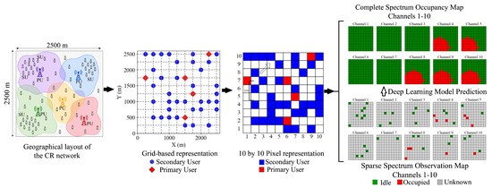
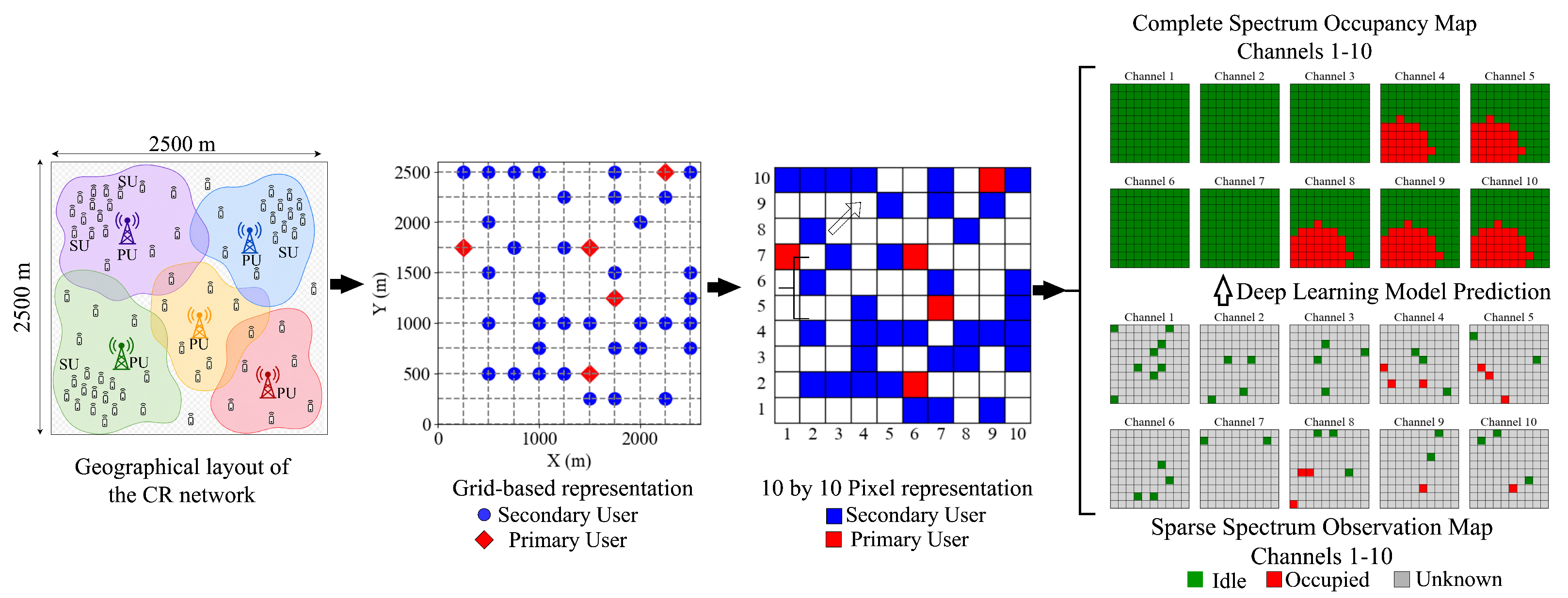
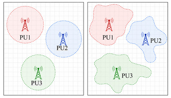
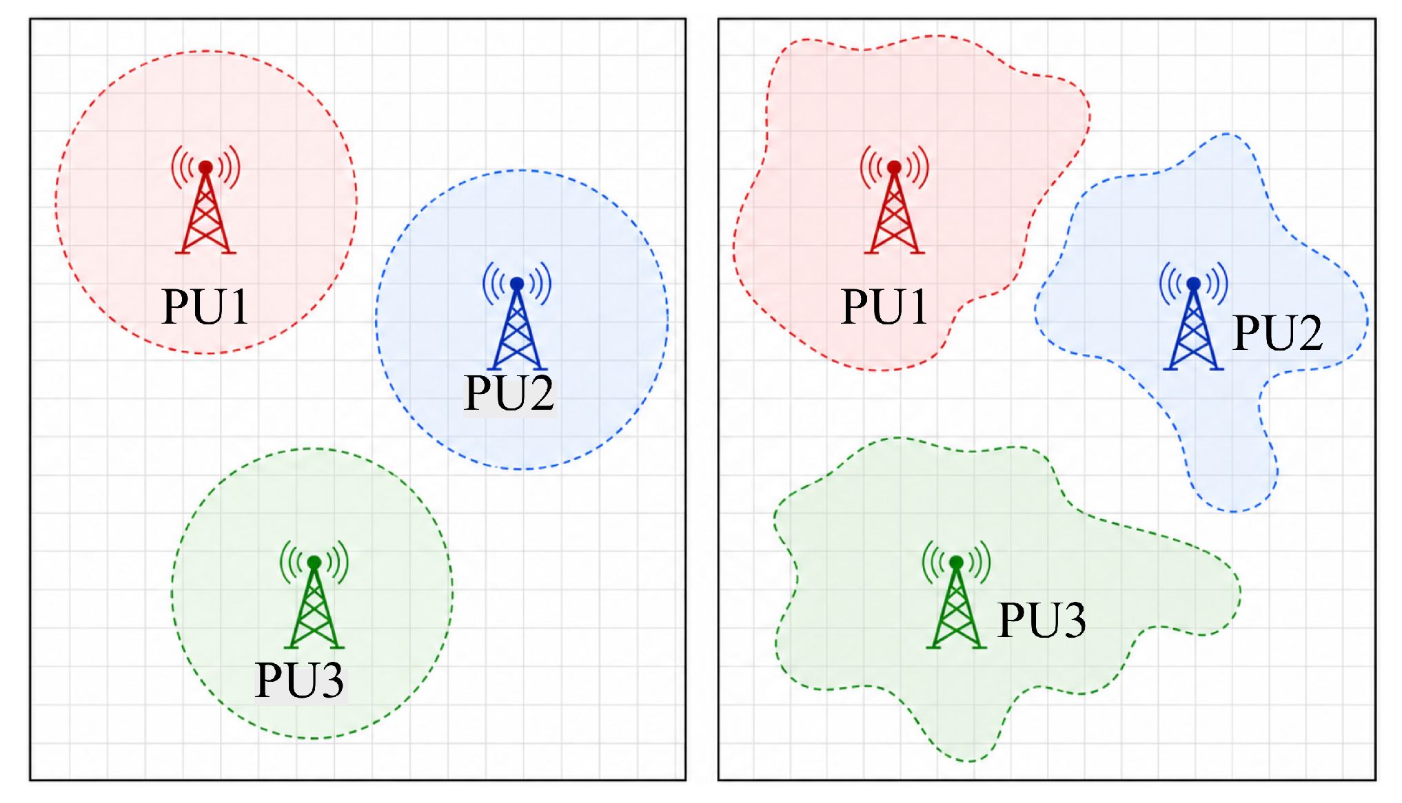
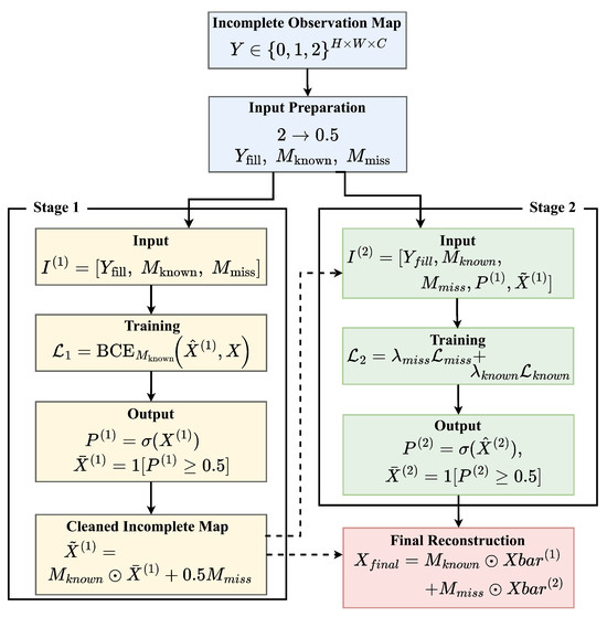
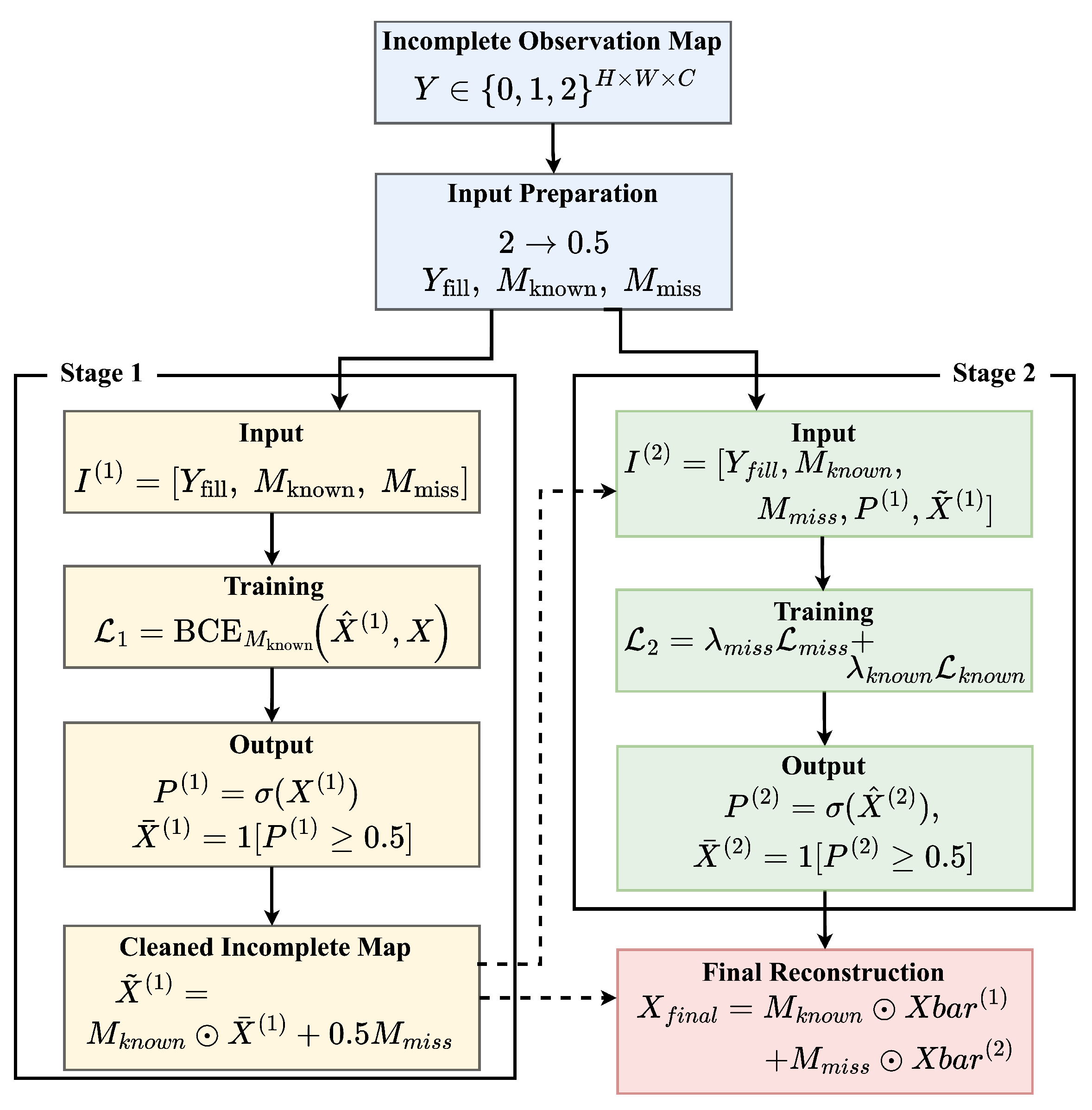
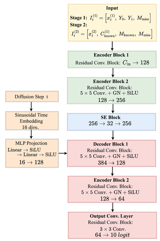
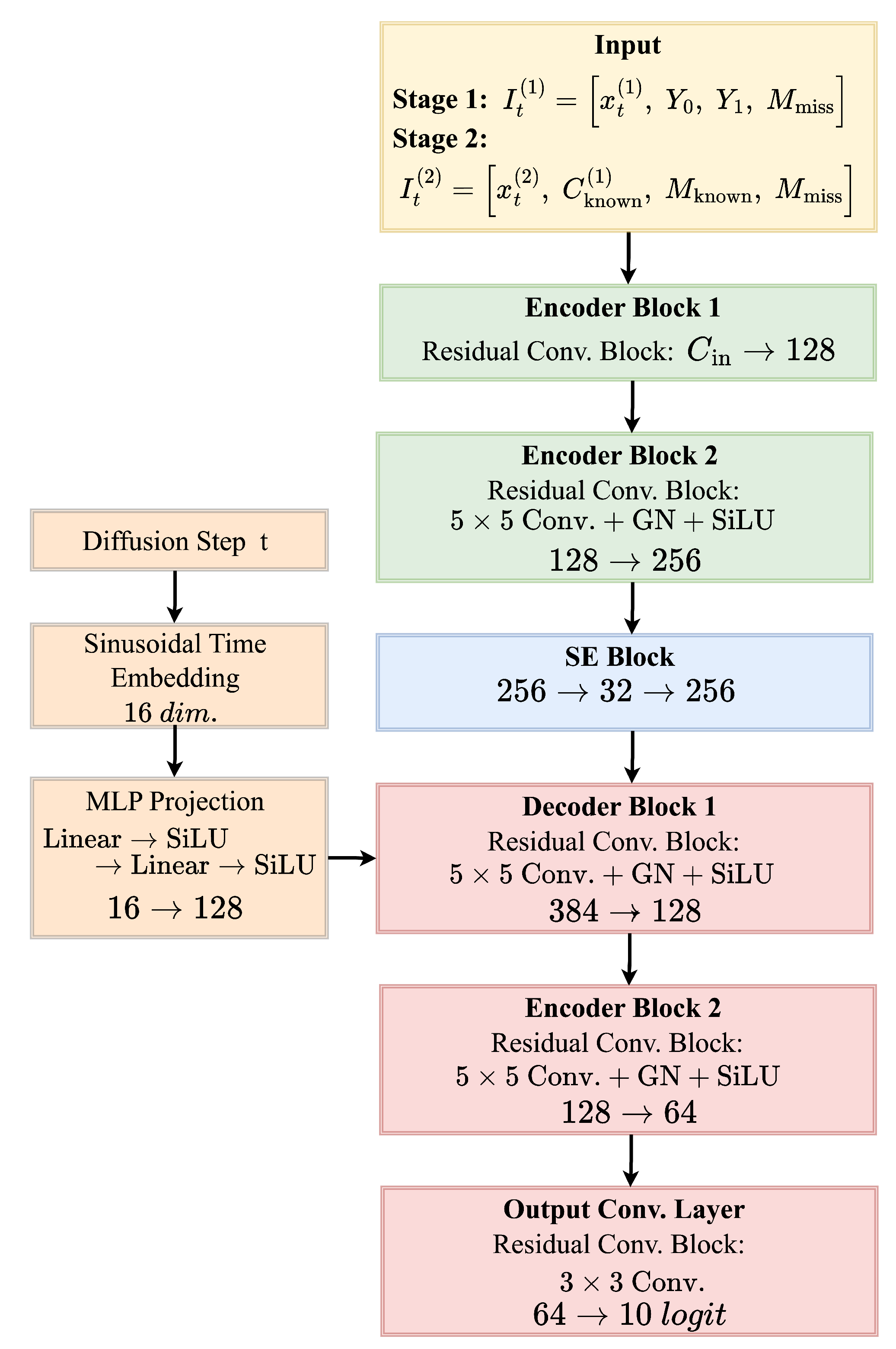
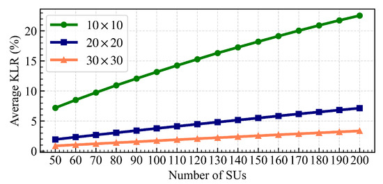
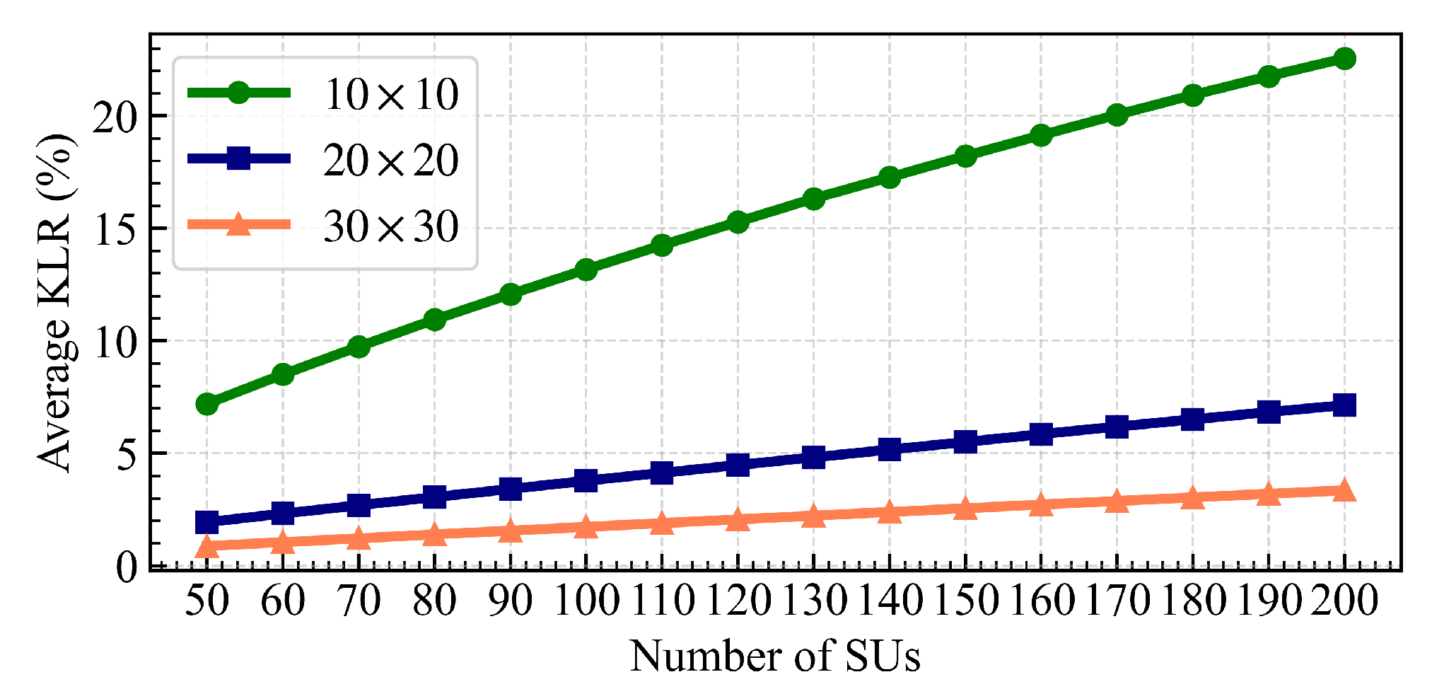
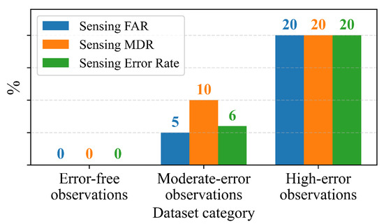
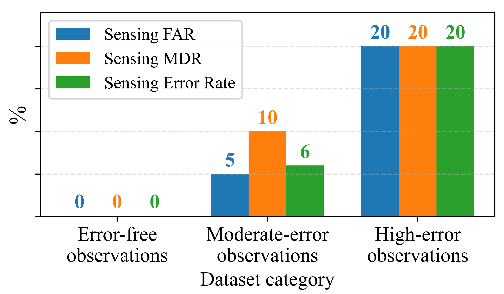
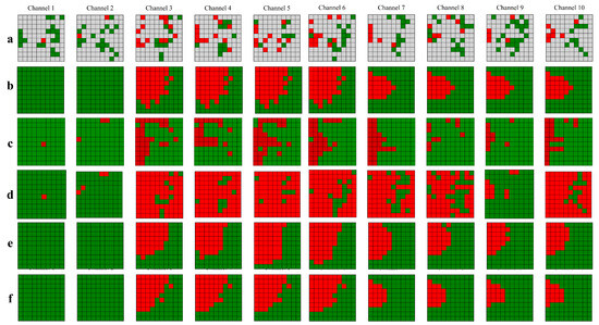
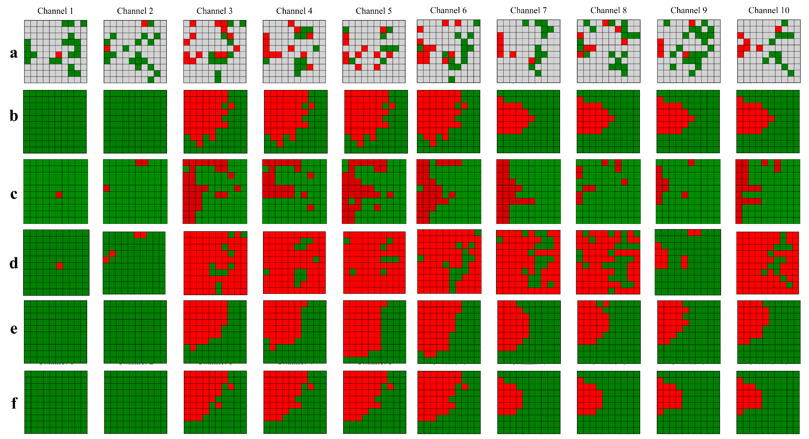
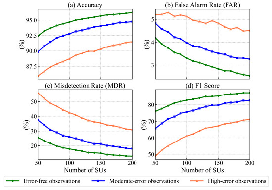
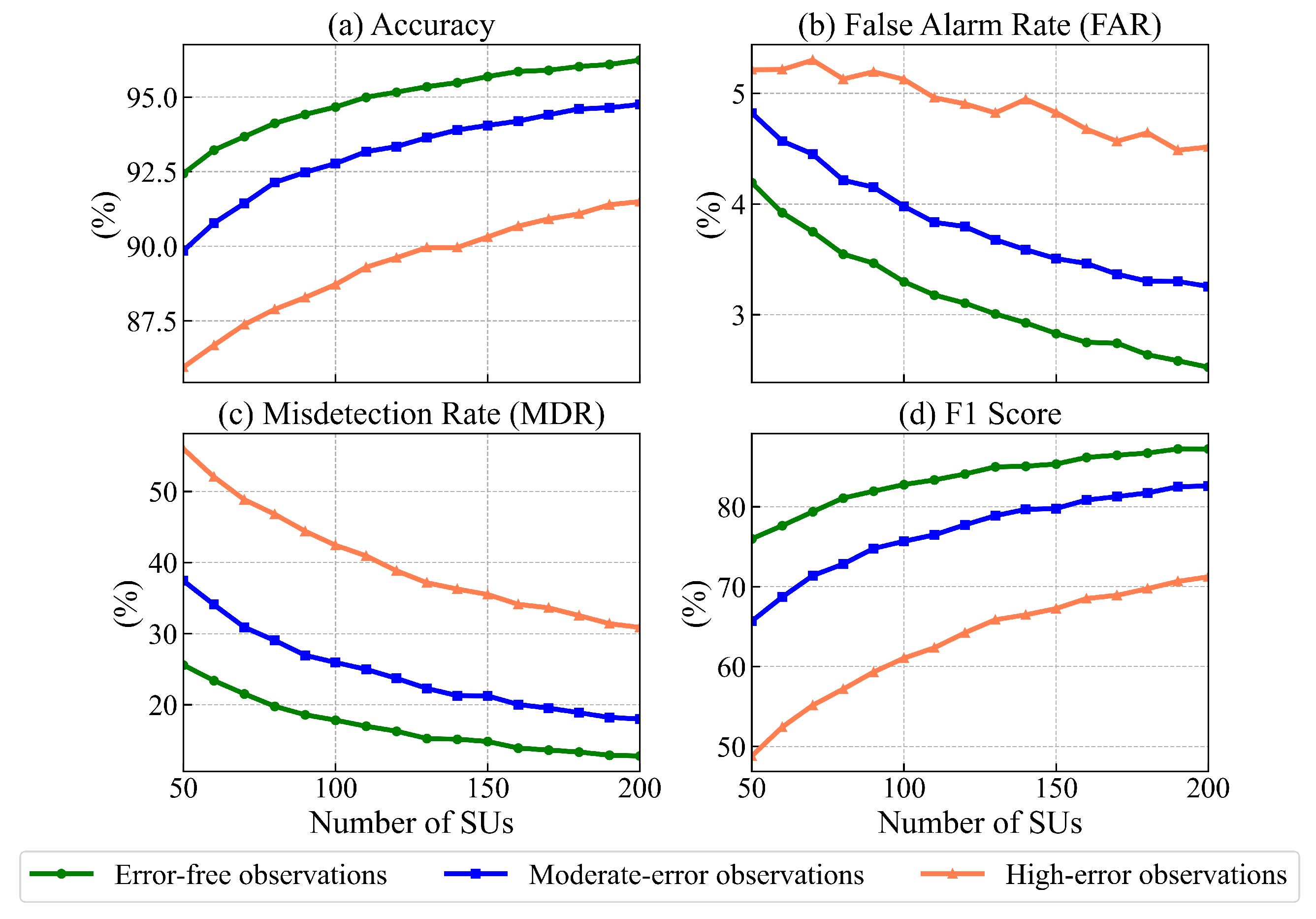
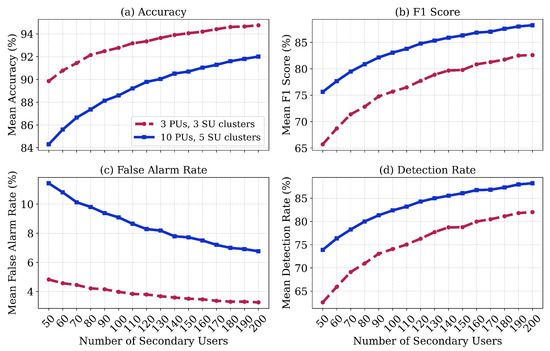
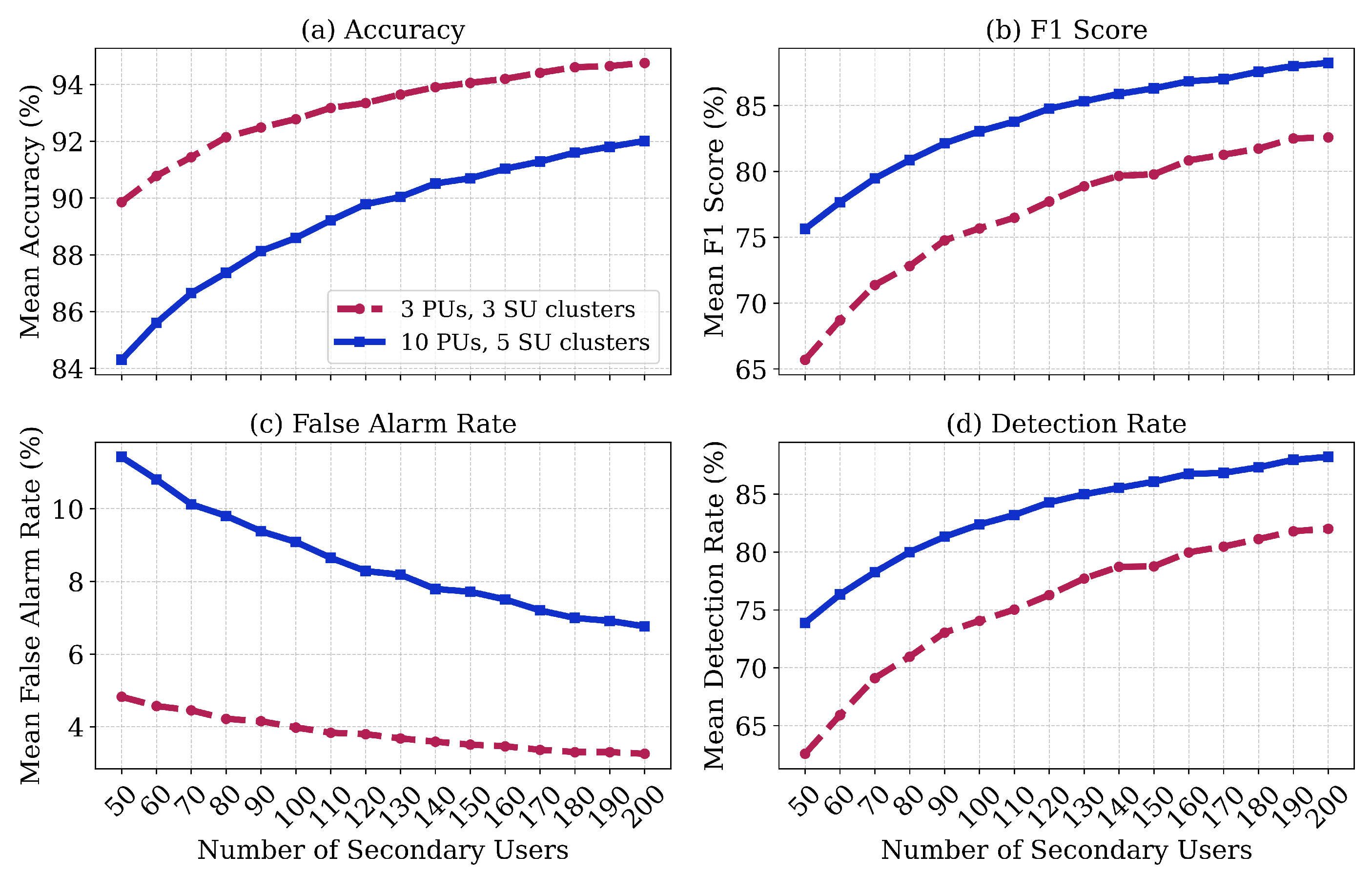
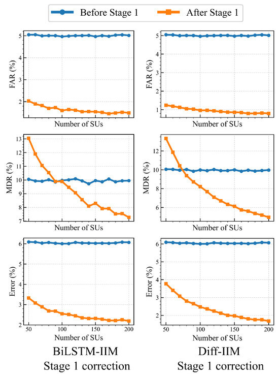
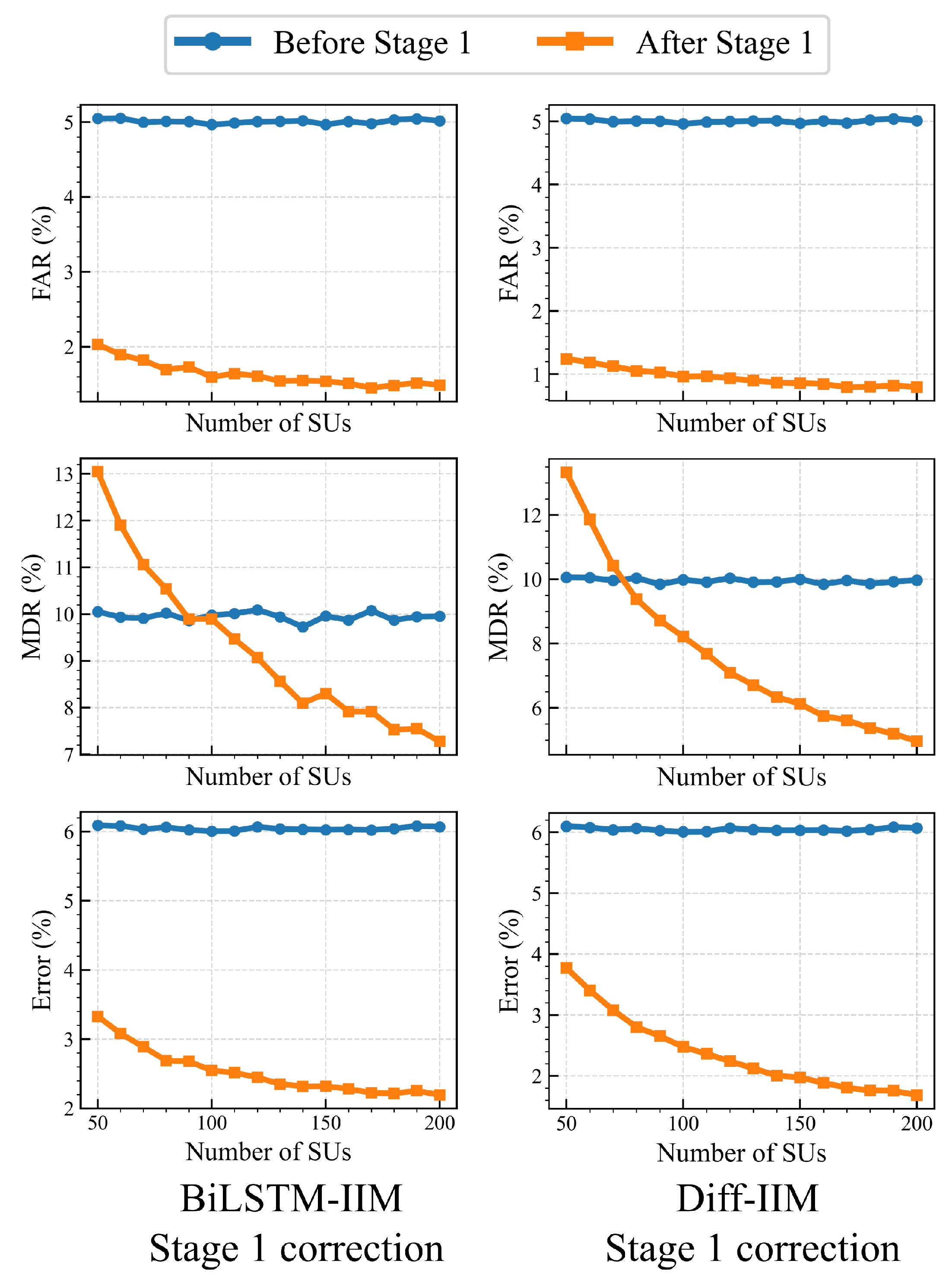
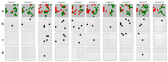
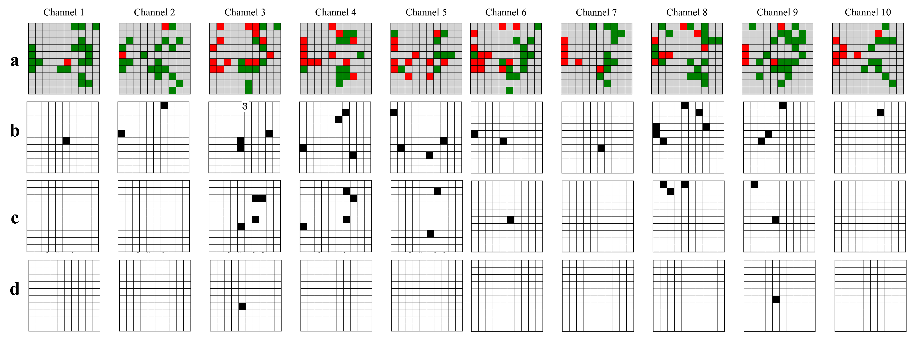
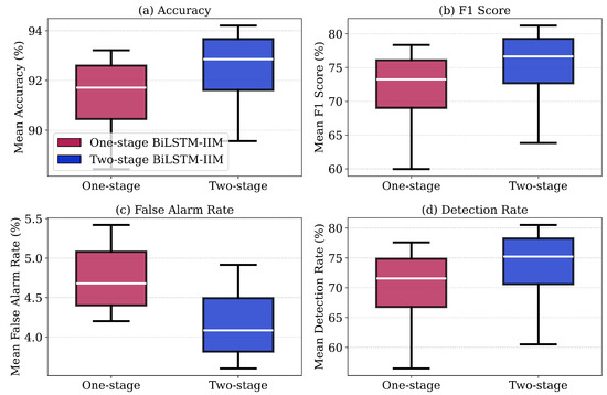
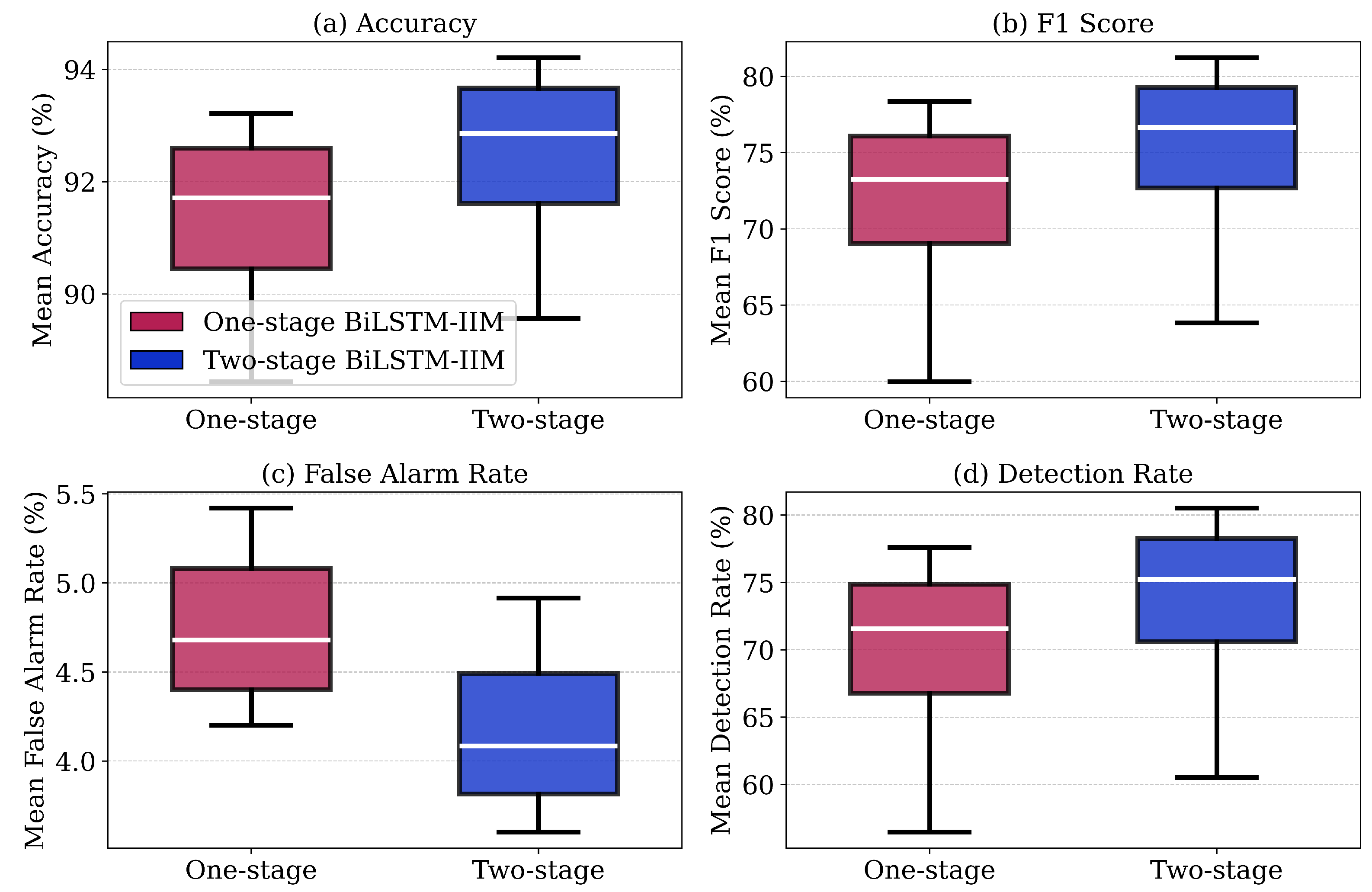

Disclaimer/Publisher’s Note: The statements, opinions and data contained in all publications are solely those of the individual author(s) and contributor(s) and not of MDPI and/or the editor(s). MDPI and/or the editor(s) disclaim responsibility for any injury to people or property resulting from any ideas, methods, instructions or products referred to in the content. |
© 2026 by the authors. Licensee MDPI, Basel, Switzerland. This article is an open access article distributed under the terms and conditions of the Creative Commons Attribution (CC BY) license.