Towards the Lowest-Carbon Home: Exploring the Effects of Building Shape, Size and Material Selection on CO₂e Embodied Emission

Abstract

The embodied emissions of buildings are expected to be limited in European Union (EU) countries; while the energy consumption of buildings is decreasing, their material footprint is becoming more significant. This article presents the results of the analysis of the embodied emissions of single-family houses, depending on their shape features and the types of construction materials used. Analysis of variance (ANOVA), Shapiro–Wilk’s test, the Kruskal–Wallis test, and Classification and Regression Trees (C&RT) are used to analyze a deterministic design-space database comprising over 35 thousand calculated scenarios and rank the importance of the houses’ features. The unit emissions (per square meter, per year) and life-long emissions of the houses are analyzed and discussed, considering the areas of the houses, their shapes, and the materials used for their construction. In planning to limit CO₂e embodied emissions, the recommendation to use life-long emissions in building assessments (to achieve better sustainability) is worked out and proved.

1. Introduction

Buildings in the EU are responsible for the highest level of raw material consumption. Under the EU Climate Law, members of the European Union are striving for climate neutrality by 2050, a goal that is likely to have the highest level of influence on the construction business in the coming years.

Buildings in the EU are also responsible for approx. 40% of the energy consumption total and 36% of energy-related greenhouse gas emissions [1]. Approx. 26% of these emissions are operational (produced during the exploration phase). The rest are embodied emissions, which are emissions associated with construction materials—from extraction, manufacturing, construction, and maintenance to the disposal phase. Over the last few years, EU legislation focused on improving the energy efficiency of buildings. Thanks to these regulations, new buildings consume less energy. The share of renewable energy in the EU’s gross final energy consumption reached 26.2% in 2025, according to provisional Eurostat data [2]. This leads to the fact that, for up-to-date buildings, embodied and operational emissions are often already equal [3]. With the new EPBD directive [4], the European Commission aims to reduce energy consumption in buildings, increase the share of renewable energy, and improve the energy standard of existing buildings. The directive also requires life cycle GWP to be calculated and disclosed for new buildings with a useful floor area exceeding 1000 m² from 2028 and for all new buildings from 2030 [4]. All these activities will increase the significance of embodied emissions, which are expected to become a more critical aspect of sustainable construction. Embodied emissions have been the subject of many scientific papers [3,5,6,7,8,9]. Recent research also applies machine learning to both emission categories; Zhang et al. [10] investigated operational emissions in urban community service units, while Fenton et al. [11] and Su et al. [12] developed approaches to predict embodied emissions.

Some countries have already implemented a commitment to calculate whole-life carbon (WLC) emissions (Denmark, Finland, France, the Netherlands, and Sweden). With the new CPR regulation [13], manufacturers of construction materials will be obliged to declare the CO₂e footprint of a material in its declaration of performance, in preparation for the potential requirements of obligatory LCAs for buildings in the future. Denmark, the Netherlands, and France have already set up threshold values for CO₂e. These requirements refer to 1 square meter of the building, similarly to the requirements for maximum primary energy consumption in other EU countries.

Existing studies address energy efficiency and promising low-carbon materials [3,6]. Recent research also examines the respective roles of material quantities and low-carbon material selection [14]. Recent studies have examined residential embodied carbon benchmarks and the influence of building geometry [15,16,17]. Further analysis is needed to evaluate the influence of building size, compactness, and sets of different construction materials simultaneously over the life cycle period. Furthermore, the critical contrast between absolute total emissions and emissions normalized by floor area is still insufficiently explored [7,8]. Although recent product-stage research identifies this relationship [17], its implications over longer life cycle periods remain insufficiently explored; larger houses may generate higher total life-long emissions (LL50) while achieving lower unit emissions (U50).

As a result of this research gap, it is not clear to policymakers and designers as to which factors have the highest influence on the total CO₂e footprint. Without an explanation of these factors, future regulations focused only on floor-area-normalized unit emissions may lead to undesirable outcomes. Because it is mathematically easier to meet per-square-meter limits in larger houses, such regulations could create an unintended incentive to design larger buildings, which would ultimately increase absolute greenhouse gas emissions. However, developer behavior is not modeled here, making this a potential regulatory consequence requiring further investigation. Meanwhile, filling the research gap on total CO₂e footprint factors by analyzing an extensive database of single-family house variants allows us to present data-driven evidence supporting the contribution of this study, which is the recommendation that limiting absolute life-long total emissions should be preferred over limiting unit emissions in order to effect true sustainability.

This article aims to analyze the CO₂e footprint of different types of buildings combined with different sets of construction materials. Single-family houses are taken into account, as it is this market segment in which the authors estimate, based on the Polish market, that 45–50% of all masonry units produced are supplied [18,19]. The article presents which building elements influence the embodied CO₂e emissions and describes why total (not per unit) emissions are also crucial for sustainable buildings. The article is focused on the following intermediate issues:

-

Comparing the life-long and the unit embodied CO₂e emissions of houses with different areas.

-

Assessing the influence of the shape and size of the building vs. the influence of the construction materials on the unit and life-long emissions.

Explaining them through the presented calculations and discussing them considering the clients’ approach allows for reasoning about which factors should be limited (by the regulations) to protect the environment more.

2. Materials and Methods

2.1. Materials

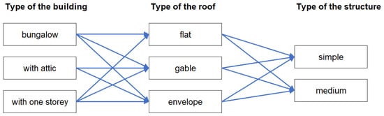
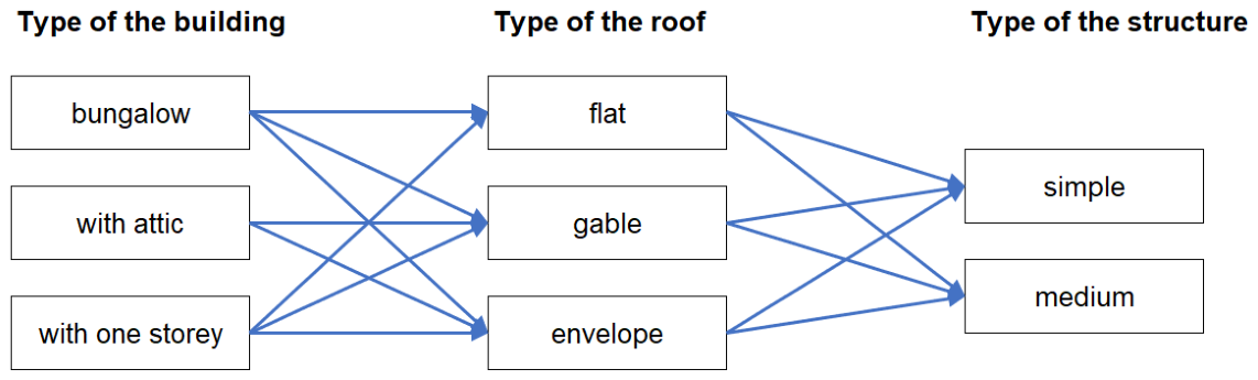
The database for an article consists of two databases combined. The first database contains the surface areas of individual partitions for various building types. The database was originally used for cost estimation and was implemented in 2018 as a web service [20]. Originally, the database included data for single-family houses with a total area of 40 to 400 m². For this article, we analyze houses with areas of 40, 70, 100, 120, 150, 180, 200, 240, and 300 m². In this study, floor area refers to the gross floor area. To ensure the functional equivalence of the compared houses, all analyzed variants provide the same basic residential function for single-family housing. Furthermore, as described later in this section, all structural and material configurations are determined to cover the exact same thermal requirements, ensuring that the buildings are functionally equivalent in terms of energy performance standards. For each area, 12 types of buildings are analyzed, as surfaces of partitions (thus embodied CO₂e emissions) strongly depend on the number of floors, types of roofs, and complexity of the shape. The types of buildings analyzed are shown in Figure 1. The simple structure was a rectangular footprint with a constant width-to-length ratio of 0.8 (where the base length is calculated as $L=\sqrt{GrossFloorArea/0.8}$). The medium structure was an L-shaped building with a garage protruding from the main body, geometrically modeled by subtracting a constant 5.5 m² from the rectangular footprint and applying an adjusted perimeter multiplier. To ensure the reproducibility of calculations, the architectural model incorporates strict geometric assumptions. The standard storey height is set to 2.8 m for each full level. The window-to-wall ratio (WWR) is defined as 20% for all bungalow and two-storey buildings, 15% for houses with an attic and a gable roof, and 10% for houses with an attic and an envelope roof. The roof slope is fixed at 25° for bungalow houses with gable roofs and 40° for houses with an attic. Based on 9 gross floor area categories and 12 distinct building geometries, 108 base building types were defined.

Figure 1. Types of analyzed buildings.

The second database consists of building materials.

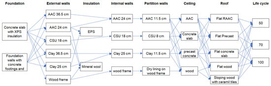
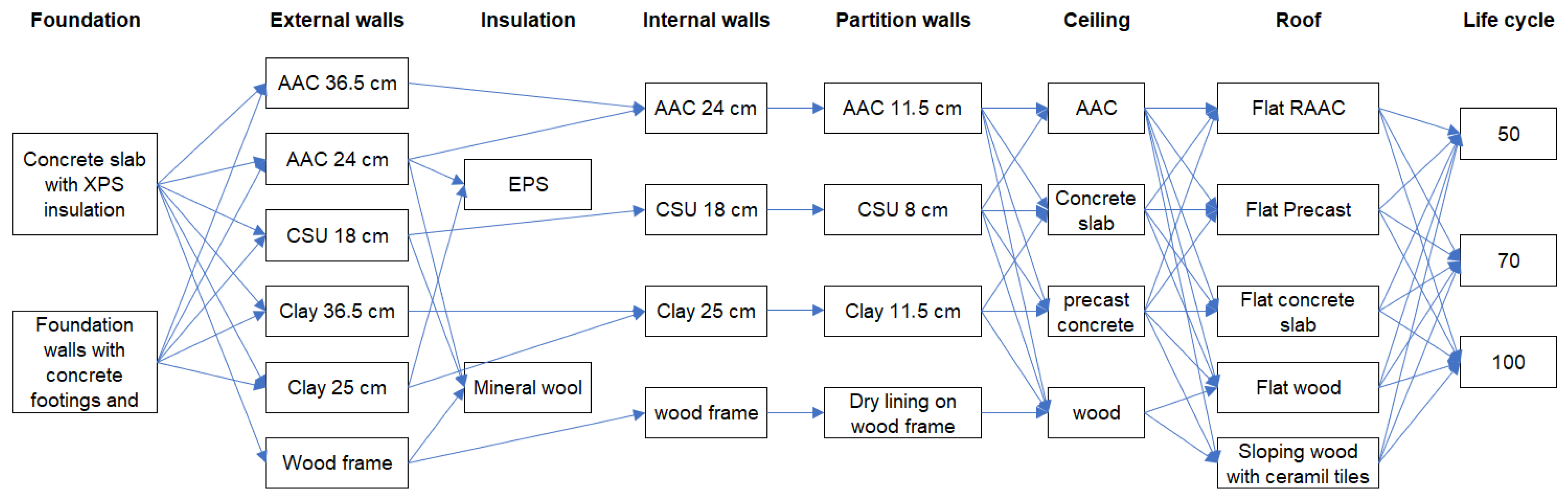
The materials used for calculation were the most popular for single-family houses in Poland. All variants are determined to meet the thermal requirements stated in national regulations [21]. Only common variants were combined, as shown in Figure 2. The more detailed description of the layers is shown in Appendix A.

Figure 2. Combination of construction materials used for building simulations.

Service life was assumed according to the [22] guidelines for each layer, and the specific replacement intervals applied to the respective components are summarized in Appendix A.

For analysis, the following modules are used:

A1: Raw material supply;

A2: Transport of raw material;

A3: Manufacture of the construction products;

B1: Use;

B4: Replacement;

C3: Waste processing;

C4: Waste disposal.

It should be pointed out that this selection of modules focuses strictly on embodied emissions. Terminology such as “life-long emissions” used in this study refers only to the sum of these specific modules over the assumed timeframe. It does not constitute a complete whole-life carbon (WLC) assessment, because operational carbon (e.g., module B6—energy use) is explicitly excluded. This boundary is maintained to keep a clear distinction between the materials’ embodied emissions and the building’s operational energy consumption.

It should also be pointed out that the data does not contain all products in the market, so the obtained calculations should be treated as estimates only. For example, only two EPDs are available for clay—one for monolithic elements with insulation in hollows and the second for standard blocks with density 575 kg/m³, that is majority of elements available on the market having higher density. The results show a significant influence from module B1, in which elements containing lime or cement have recarbonation calculated. Calculation of module B4 may also have a considerable impact, as it is essential to know how often particular materials need replacing.

All materials were calculated for 3 service life periods: 50, 70, and 100 years. Fifty years of service life results from the new EPBD directive. This likely reflects European standards, where 50 years is the service life of residential buildings [23]. It does not mean that the building will exist only for an assumed period; rather, it is the time after which renovation may be required. Two other periods were analyzed as, in 2021, the age of 38% of residential buildings in Poland exceeded 50 years [24]. Regarding sustainability, buildings should be designed for a more extended period.

It should be pointed out that this study is a deterministic design-space analysis. The true unit of analysis is a calculated scenario, not an independent statistical observation of an existing building. In this article, a design “variant” means a feasible combination of a building shape and construction materials. A calculated “scenario” is a variant calculated for a specific life cycle period (50, 70, or 100 years). The combinations were generated according to strict component-existence and structural compatibility rules. First, the 9 gross floor areas were combined with 12 building geometries, providing 108 base architectural types. Next, they were combined with the material configurations shown in Figure 2. The algorithm filtering the design-space database excluded structurally or architecturally incompatible combinations to ensure realistic models. For instance, specific roof finishes were strictly tied to their geometric types; flat roof layers (e.g., EPDM membranes) were exclusively assigned to flat roof geometries, whereas sloping roofs with ceramic tiles were assigned solely to gable or envelope geometries. Furthermore, structural safety exclusions were applied, such as preventing the placement of heavy reinforced concrete roofs or ceilings on light wood-frame walls. This algorithmic filtering procedure resulted in exactly 1323 admissible and structurally feasible material-geometry combinations for each of the 9 house-area groups. Consequently, the total number of valid design variants exactly amounts to 11,907 (9 area groups × 1323 variants). Calculated for 3 life cycle periods, the final database consists of 35,721 deterministic scenarios.

Environmental product declarations for particular materials were obtained from online databases [25,26,27]. As EPDs from different sources may differ significantly, a basic harmonization and selection procedure was applied to ensure the comparability of the data. First, only valid declarations based on the EN 15804 standard [28] and relevant Product Category Rules (PCR) were selected. To ensure geographical consistency, EPDs representing materials produced in Germany and Poland were prioritized, which allowed for a relatively consistent assumption regarding the electricity mix and production technology. Next, the declared units from various EPDs were recalculated to match the specific volume or area of the partitions analyzed in this study, taking into account the typical density and moisture content of the materials used. Despite this selection process, it must be noted that combining several databases always carries a risk of minor methodological discrepancies, such as differences between EN 15804+A1 and +A2 [28,29] versions or the specific treatment of biogenic carbon. These factors are considered an inherent limitation of the current EPD system.

2.2. Methods

2.2.1. Assessing Means of Samples with ANOVA

The created set of data allows for many analyses. Initially, the analysis of variance (ANOVA) [30] was selected to compare the groups of houses’ structures against the total built-in emission and the unit CO₂e emission. ANOVA was successfully applied to many problems, e.g., in [31,32,33]. The statistics $F$ is calculated there and compared to $F_{\alpha }$ (read from Fisher’s distribution), which depends on the assumed confidence level $\alpha$, ${df}_{btw}$, and ${df}_{tot}$. Degrees of freedom (${df}_{btw}$ and ${df}_{tot}$) are defined as:

$${df}_{btw}=k-1$$

(1)

$${df}_{tot}=n-k$$

(2)

where

$n$ is the total number of cases in all samples;

$k$ is the number of different samples to which the sample cases belong.

The null hypothesis $H_0$ (about the equality of means calculated for each sample) cannot be rejected only if $F<F_{\alpha }$. The application of ANOVA requires the following conditions to be met [34,35]:

-

Independence of random variables for each population;

-

Measurability of variables;

-

Normality of distribution of random variables in each population;

-

Variance homogeneity in all populations.

Based on [36], it can be stated that the independence and the measurability of all cases in the created database are provided. The powerful test of normality [37] of the sample is the Shapiro–Wilk test [38]. It is applied in a variety of analyses, e.g., in [39,40]. The following hypotheses are tested there:

H₀. 

Values of the examined parameter are normally distributed.

H₁. 

The distribution of these values is not normal.

The statistics $W$ is calculated for this test based on the formula:

$$W={\displaystyle \frac{{\left[{\displaystyle {\sum }_{i=1}^{n/2}}{a}_{ni}(x_{n-i+1}-x_{\left(i\right)})\right]}^2}{{\displaystyle {\sum }_{i=1}^n}{(x_i-\overline{x})}^2}}$$

(3)

where

$x_i$—non-ordered values in the sample;

$x_{\left(i\right)}$—values in the sample ordered increasingly;

$\overline{x}$—mean value;

$n$—number of values in the sample;

$n/2$—total part of $n$ divided by 2;

$a_{n,i}$—tabularized coefficient dependent on $n$.

Then, the calculated test statistics $W$ is compared to the theoretical $W_{th}$, which depends on $n$ and the confidence level $\alpha$. If $W>W_{th}$ there is no reason to reject the null hypothesis $H_0$ (about the normal distribution of the sample). The Statistica 13 software (by Tibco), instead of $W$ comparison, returns the $p$ value. If $p>\alpha ,$ then also $W>W_{th}$. So, the normality is confirmed then. This confirmation is necessary before confirming the ANOVA application’s last condition, i.e., the homogeneity of variances of the compared samples. It can be done with Levene’s test [41], which was widely discussed, e.g., [42,43], and successfully applied, e.g., in [44,45]. Similarly to ANOVA, the $W$ statistics is compared to the theoretical value based on Fisher’s distribution $F$, which is confidence level $\alpha$, and degrees of freedom, i.e., $k-1$ and $n-k$ dependent. However, the test statistics is calculated based not on $x_{ij}$ values (like in ANOVA) but based on the $z_{ij}$ values calculated as

$$z_{ij}=\left|x_{ij}-\overline{x_{\mathsf{ı}}}\right|$$

(4)

where

$x_{ij}$ is a $j$ value in $i$ sample;

$\overline{x_{\mathsf{ı}}}$ is mean value in $i$ sample;

${\overline{z}}_i$ is a mean value of $z_{ij}$ in $i$ sample, given by the following formula:

If $W>F,$ the null hypothesis is accepted (about the homogeneity of variances) of analyzed samples.

However, during analyses, it has occurred that, for the majority of attempts to compare the subsets of the prepared database, the normal character of the subsets cannot be confirmed with Shapiro–Wilk’s test (see the exemplary result in Table 1).

Table 1. Shapiro–Wilk’s test results.

House Area	Number of Types of Houses’ Structures	Value W (Shapiro–Wilk Test)	p Value
40 U	1322	0.993617	0.000019
40 LL	1322	0.993617	0.000019
70 U	1323	0.977881	0.000000
70 LL	1323	0.977881	0.000000
100 U	1322	0.969347	0.000000
100 LL	1322	0.969347	0.000000
120 U	1323	0.972001	0.000000
120 LL	1323	0.972001	0.000000
150 U	1323	0.96557	0.000000
150 LL	1323	0.96557	0.000000
180 U	1323	0.960173	0.000000
180 LL	1323	0.960173	0.000000
200 U	1323	0.947964	0.000000
200 LL	1323	0.947964	0.000000
240 U	1323	0.944413	0.000000
240 LL	1323	0.944413	0.000000
300 U	1323	0.931129	0.000000
300 LL	1323	0.931129	0.000000

The “U” label of the subsets means that the unit emission values are considered. The “LL” label indicates that lifelong emissions are considered. The p values are below the assumed $\alpha =0.05$, so the alternative $H_1$ hypothesis should be accepted, i.e., the normal character of all these samples is not confirmed. That has excluded the possibility of ANOVA application (and the necessity of the homogeneity verification with Levene’s test). Therefore, the nonparametric Kruskal–Wallis test is used to compare subsets.

2.2.2. Kruskal–Wallis Test

Because the samples—types of houses—are generated, not observed, it is understandable that the sample distribution may not be normal. Then the Kruskal–Wallis test is helpful to assess the differences between subsets of the samples. The Kruskal–Wallis’ test [46] is the nonparametric one, i.e., it can be applied to non-normally distributed samples. It is based on the Mann–Whitney U test (also called the Wilcoxon rank-sum test) [47], which is dedicated to comparing just two samples. The Kruskal–Wallis test can be applied to a maximum of 10 samples [35]. The values of the sample are ranked separately for each sample, and only ranks are used to calculate the statistics $H$.

$$H=\left({\displaystyle \sum _{i=1}^k}{n}_i-1\right){\displaystyle \frac{{\left[{\displaystyle {\sum }_{i=1}^k}{n}_i\left(\overline{r_{\mathsf{ı}}}-\overline{r}\right)\right]}^2}{{\displaystyle {\sum }_{i=1}^k}{\displaystyle {\sum }_{j=1}^{n_i}}{\left(r_{ij}-\overline{r}\right)}^2}}$$

(5)

where

$k$—number of analyzed samples;

$n_i$—number of values in the sample $i$;

$r_{ij}$—the rank of $j$ observation is $i$ sample;

$\overline{r}$—the average of all $r_{ij}$ given by the formula

$$\overline{r}={\displaystyle \frac{{\displaystyle {\sum }_{i=1}^k}{n}_i+1}{2}}$$

(6)

and

$\overline{r_i}$—the average rank of all observations in $i$ sample given by the formula

$$\overline{r_i}={\displaystyle \frac{{\displaystyle {\sum }_{j=1}^{n_i}}{r}_{ij}}{n_i}}$$

(7)

Then the statistics $H$ is compared to the corresponding critical value $H_c$, which depends on the confidence level $\alpha$ and can be read from the tables. If the statistics is significant, i.e., $H>H_c$, the null hypothesis is rejected. That means that there is stochastic dominance between the two samples. Then, the pairwise comparison between the two samples is suggested. The Statistica software returns $p$ value. If $p<\alpha ,$ then $H>H_c$. Considering the successful application of the Kruskal–Wallis test, e.g., in [48,49], it is decided to use just this test to confirm the statistical importance of the difference between the analyzed subsets.

For comparisons of the same building variants calculated for two different service-life periods (50 and 100 years), the observations are paired rather than independent. Therefore, these comparisons were performed using the Wilcoxon signed-rank test for paired samples. We applied the test separately to unit emissions (U50 vs. U100) and total life-long emissions (LL50 vs. LL100). Statistical significance was assumed at p < 0.05. The magnitude of the paired difference was additionally quantified using the effect size r, calculated as |Z|/√N. In contrast, comparisons among the nine independent house-area groups were performed using the Kruskal–Wallis test followed by Dunn’s post hoc comparisons with Holm adjustment.

2.2.3. Classification and Regression Trees (C&RT)

Breiman et al. popularized the decision trees [50]. They are also called Classification and Regression Trees (C&RT) or simply decision trees (DT). If several features describe the analyzed phenomenon and many (hundreds or thousands) observations are recorded, this classifying (or predicting) tool as C&RT can be applied. The dataset is split into subsets in the node so-called leaves. The user can specify the stop-split criterion by giving a minimal number of recorded cases (rows in the database). The node becomes the end-leaf if there is no split in a specific node. Based on the analysis of the end leaves, the predicted class or the predicted value can be read. There are so many splits possible—the independent variables describing the analyzed phenomenon can be numbers but also categories and metaheuristics are involved in finding the best splitting criteria aiming at the most accurate predictions (in regression problems) or the most accurate classifications (in classification problems). If DT is used for a classification problem, it produces the ranking of features, which is transformed into the list of relative importance [51,52,53]. This ranking is based on the number of times that a certain feature is used in the tree as a criterion in a leaf, and it is based on the number of cases that belong to or pass through these leaves [54]. This ability of a machine learning tool for creating the ranking of importance of the influence of the independent variables on the output, i.e., on the dependent variable, is named as “feature importance”. As the results of feature importance achieved through C&RT are proven, e.g., in [55,56], it is decided to utilize this in the article based on Statistica software (by Tibco).

3. Results

3.1. Life Long vs. Unit Emissions

To make the results (especially figures and tables) easy to read, the following abbreviations and labeling are applied:

U for the unit embodied CO₂e emission per year, per m² of a house, in kilograms;

LL for the total embodied CO₂e emission in the lifetime of a house, in kilograms;

50 for the 50-year life cycle of a house;

100 for the 100-year life cycle of a house;

Then, e.g., label U50 means cases grouped by the unit emission calculated based on 50 years of the houses’ life cycle.

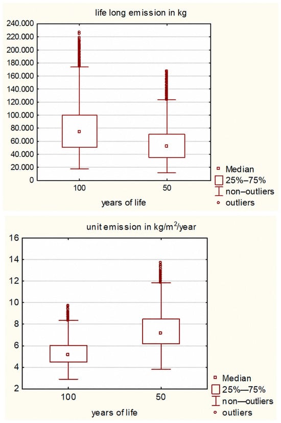
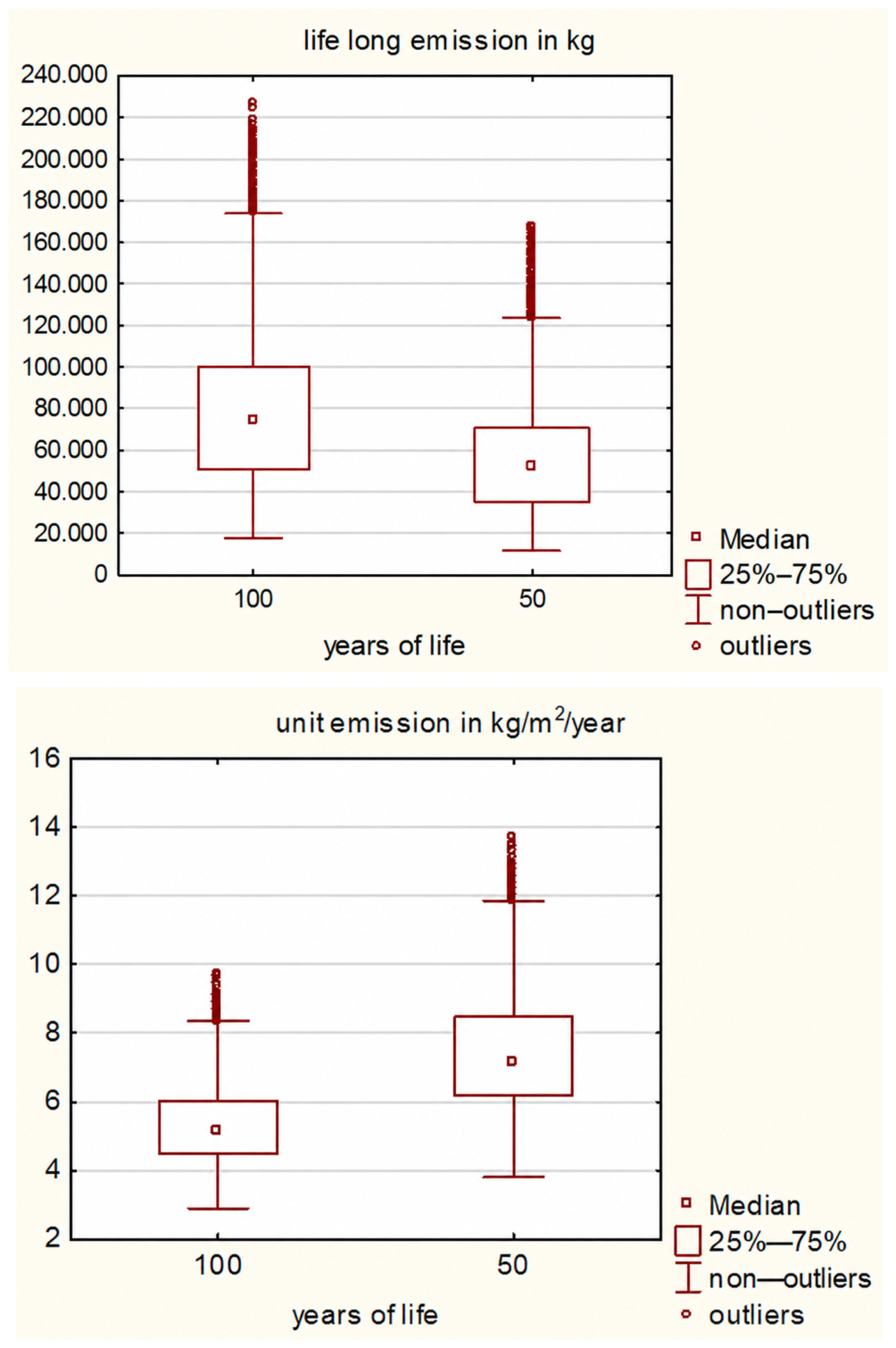
The basic statistics for the CO₂e emissions are presented in Table 2. The comparisons of unit emissions and life-long emissions based on 50- and 100-year house life cycles are presented in Figure 3.

Table 2. Unit and life-long emissions—basic statistics.

Sample	Number of Types of Houses’ Structures	Mean	Minimum	Maximum	Standard Deviation
U50	11,907	7430	3798	13,695	1647
LL50	11,907	54,530	11,940	168,195	26,018
U100	11,907	5316	2899	9740	1122
LL100	11,907	77,712	17,563	227,035	35,862

Figure 3. The comparison of LL100 to LL50 emission and U100 to U50 emissions for all 11,907 types of the houses’ structures.

The comparison between the 50-year and 100-year life-cycle scenarios involves paired observations, because each value calculated for a 50-year service life has a directly corresponding value for the same building variant calculated for a 100-year service life. Therefore, we used the Wilcoxon signed-rank test for paired samples instead of a test for independent groups.

As expected, total life-long embodied emissions increase with the assumed service life. The median LL emission increased from 51,764.26 kg CO₂e for LL50 to 74,284.48 kg CO₂e for LL100. The median paired increase was 22,086.18 kg CO₂e. LL100 was higher than LL50 for all 11,907 analyzed building variants. The Wilcoxon signed-rank test confirmed that the difference was statistically significant (W = 0, p < 0.001), with a large effect size (r = 0.866) (Table 3). This increase results mainly from replacing or renovating building components during the longer service-life period.

Table 3. Wilcoxon signed-rank test results for paired LL50 and LL100 emissions.

Sample	Sample Size	Median LL50 in kg	Median LL50 in kg	Median Paired Difference LL100−LL50) in kg	W	p	Effect Size r
LL50 vs. LL100	11,907	51,764.26	74,284.48	22,086.18	0	<0.001	0.866

A different relationship was observed for unit embodied emissions expressed per square meter and year. The median unit emission decreased from 7.192 kg CO₂e/(m²·year) for U50 to 5.144 kg CO₂e/(m²·year) for U100, corresponding to a median paired decrease of 2.055 kg CO₂e/(m²·year). U100 was lower than U50 for all 11,907 corresponding building variants. The Wilcoxon signed-rank test confirmed that this reduction was statistically significant (W = 0, p < 0.001), again with a large effect size (r = 0.866) (Table 4).

Table 4. Wilcoxon signed-rank test results for paired U50 and U100 emissions.

Sample	Sample Size	Median U50 in kg/m2/year	Median LL50 in kg/m2/year	Median Paired Difference LL100−LL50) in kg/m2/year	W	p	Effect Size r
U50 vs. U100	11,907	7.192	5.144	2.055	0	<0.001	0.866

These results demonstrate that extending the assumed building service life has opposite effects on the two emission indicators: absolute life-long embodied emissions increase, whereas annualized unit emissions decrease. Consequently, assessing a building’s environmental performance may lead to different conclusions depending on whether you consider absolute life-long emissions or emissions normalized by floor area and service life.

3.2. Emissions Grouped by the Houses’ Areas

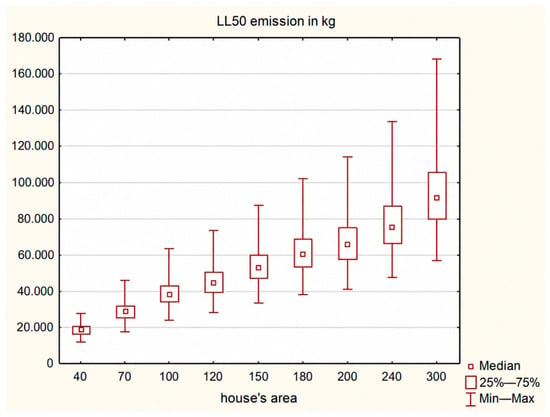
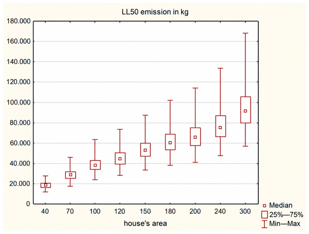
The distributions of the LL50 emissions for the houses of different areas are presented in Figure 4.

Figure 4. The comparison of the distribution of LL50 emissions for the houses of different areas.

Differences among the nine house-area groups (40, 70, 100, 120, 150, 180, 200, 240, and 300 m²) are assessed using the Kruskal–Wallis test. Following a significant omnibus result, pairwise comparisons are performed using Dunn’s post hoc test [57,58]. To control the family-wise error rate across the 36 pairwise comparisons, p-values are adjusted using the Holm [59] procedure. Effect magnitude for pairwise comparisons was quantified using Cliff’s delta (δ), with 95% confidence intervals estimated by nonparametric bootstrap resampling (1000 replicates) [60]. Medians and interquartile ranges (Q1–Q3) are reported as descriptive statistics. Statistical significance is set at adjusted p < 0.05 (see Table 5 and Table 6).

Table 5. Descriptive statistics of LL50 for the nine house area groups included in the Kruskal–Wallis analysis.

House Area	n	Median	Q1	Q3	IQR
40	1323	18,667.98	16,740.92	20,536.68	3795.76
70	1323	28,602.54	25,533.65	31,809.53	6275.88
100	1323	38,145.48	33,925.87	42,886.75	8960.88
120	1323	44,405.84	39,611.10	50,329.20	10,718.10
150	1323	52,671.17	46,805.97	59,676.29	12,870.32
180	1323	60,333.01	53,526.08	68,651.03	15,124.94
200	1323	65,526.73	57,769.81	74,866.85	17,097.04
240	1323	75,659.36	66,591.79	86,583.04	19,991.26
300	1323	91,511.20	79,544.76	105,760.18	26,215.41

Table 6. Dunn’s post hoc pairwise comparisons between house area groups with Holm-adjusted p-values and Cliff’s delta effect sizes.

Area 1 [m2]	Area 2 [m2]	Median Difference	Holm-Adjusted p	Cliff’s δ	95% CI Lower	95% CI Upper
40	70	−9934.56	<0.001	−0.950	−0.959	−0.940
40	100	−19,477.50	<0.001	−1.000	−1.000	−1.000
40	120	−25,737.86	<0.001	−1.000	−1.000	−1.000
40	150	−34,003.19	<0.001	−1.000	−1.000	−1.000
40	180	−41,665.03	<0.001	−1.000	−1.000	−1.000
40	200	−46,858.76	<0.001	−1.000	−1.000	−1.000
40	240	−56,991.38	<0.001	−1.000	−1.000	−1.000
40	300	−72,843.23	<0.001	−1.000	−1.000	−1.000
70	100	−9542.94	<0.001	−0.762	−0.787	−0.738
70	120	−15,803.30	<0.001	−0.932	−0.942	−0.921
70	150	−24,068.63	<0.001	−0.989	−0.992	−0.986
70	180	−31,730.47	<0.001	−0.999	−0.999	−0.998
70	200	−36,924.19	<0.001	−1.000	−1.000	−1.000
70	240	−47,056.82	<0.001	−1.000	−1.000	−1.000
70	300	−62,908.66	<0.001	−1.000	−1.000	−1.000
100	120	−6260.36	<0.001	−0.463	−0.498	−0.426
100	150	−14,525.69	<0.001	−0.797	−0.819	−0.775
100	180	−22,187.53	<0.001	−0.931	−0.941	−0.919
100	200	−27,381.25	<0.001	−0.970	−0.976	−0.963
100	240	−37,513.88	<0.001	−0.995	−0.997	−0.993
100	300	−53,365.72	<0.001	−1.000	−1.000	−1.000
120	150	−8265.33	<0.001	−0.495	−0.536	−0.456
120	180	−15,927.17	<0.001	−0.772	−0.797	−0.746
120	200	−21,120.89	<0.001	−0.881	−0.898	−0.865
120	240	−31,253.52	<0.001	−0.967	−0.973	−0.960
120	300	−47,105.36	<0.001	−0.997	−0.998	−0.996
150	180	−7661.84	<0.001	−0.402	−0.441	−0.365
150	200	−12,855.56	<0.001	−0.615	−0.647	−0.585
150	240	−22,988.19	<0.001	−0.842	−0.861	−0.822
150	300	−38,840.03	<0.001	−0.967	−0.973	−0.960
180	200	−5193.72	<0.001	−0.265	−0.305	−0.225
180	240	−15,326.35	<0.001	−0.613	−0.645	−0.580
180	300	−31,178.19	<0.001	−0.880	−0.896	−0.864
200	240	−10,132.63	<0.001	−0.394	−0.430	−0.354

The Kruskal–Wallis test reveals significant differences among the nine house-area groups, H(8) = 10,175.37, p < 0.001, with a large overall effect (ε² = 0.855). Dunn’s post hoc pairwise comparisons with Holm adjustment confirm statistically significant differences between all 36 pairs of house-area groups (all adjusted p < 0.001). The magnitude of pairwise differences varies considerably, as indicated by Cliff’s δ (Table 6).

Pairwise comparisons are performed using Dunn’s post hoc test following a significant Kruskal–Wallis test. P-values are adjusted for multiple comparisons using the Holm procedure. Cliff’s δ is reported as a measure of effect size together with its 95% confidence interval. Only the 36 unique pairwise comparisons are presented. The Kruskal–Wallis test indicates a statistically significant difference among the nine house-area groups, H(8) = 10,175.37, p < 0.001. The global effect is large (ε² = 0.855). Median LL50 increased monotonically with house area, from 18,667.98 for 40 m² to 91,511.20 for 300 m². Dunn’s post hoc tests with Holm adjustment show statistically significant differences for all 36 pairwise comparisons (all adjusted p < 0.001). Pairwise effect sizes vary substantially: Cliff’s δ ranged in absolute magnitude from 0.265 for the 180 vs. 200 m² comparison to approximately 1.000 for several widely separated area groups, indicating that statistical significance is accompanied by effects ranging from modest to near-complete separation of distributions.

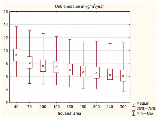
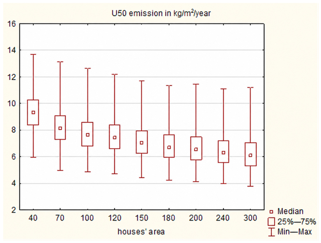
A similar set of calculations is prepared for the unit emissions. Figure 5 presents the box plots for these houses’ areas.

Figure 5. The comparison of the distribution of U50 emissions for the houses of different areas.

The distribution of unit embodied CO₂e emissions is analyzed across nine house-area groups ranging from 40 to 300 m². Descriptive statistics reveal a clear monotonic decrease in unit emissions with increasing house area (Table 7). The median value decreases from 9.334 for the smallest houses (40 m²) to 6.101 for the largest houses (300 m²), corresponding to a reduction of approximately 34.6%. This pattern suggests that, although larger houses generate higher total embodied emissions, the embodied emission burden per unit of floor area and year decreases as house size increases.

Table 7. Descriptive statistics of unit embodied CO₂e emissions by house-area group U50.

House Area	n	Median	Q1	Q3	IQR
40	1323	9.334	8.370	10.268	1.898
70	1323	8.172	7.295	9.088	1.793
100	1323	7.629	6.785	8.577	1.792
120	1323	7.401	6.602	8.388	1.786
150	1323	7.023	6.241	7.957	1.716
180	1323	6.704	5.947	7.628	1.681
200	1323	6.553	5.777	7.487	1.710
240	1323	6.305	5.549	7.215	1.666
300	1323	6.101	5.303	7.051	1.748

The Kruskal–Wallis test confirms statistically significant differences in unit embodied CO₂e emissions among the nine house-area groups, H(8) = 3489.56, p < 0.001. The associated effect size is ε² = 0.293, indicating that house area accounted for a substantial proportion of the variability in ranked unit embodied emissions. The magnitude of this effect is, however, considerably smaller than that observed for total embodied CO₂e emissions (Table 8).

Table 8. Pairwise comparisons of unit embodied CO₂e emissions between house-area groups using Dunn’s post hoc test with Holm adjustment.

Comparison (m2)	Median Diff.	Dunn Z	Holm-Adjusted p	Cliff’s δ	95% CI
40 vs. 70	1.162	13.368	<0.001	0.417	0.379–0.454
40 vs. 100	1.705	21.208	<0.001	0.582	0.548–0.615
40 vs. 120	1.933	24.519	<0.001	0.648	0.615–0.680
40 vs. 150	2.311	31.239	<0.001	0.741	0.712–0.766
40 vs. 180	2.630	36.547	<0.001	0.798	0.774–0.821
40 vs. 200	2.781	37.991	<0.001	0.798	0.774–0.820
40 vs. 240	3.029	42.265	<0.001	0.836	0.815–0.857
40 vs. 300	3.233	45.367	<0.001	0.848	0.828–0.869
70 vs. 100	0.543	7.840	<0.001	0.213	0.171–0.255
70 vs. 120	0.771	11.152	<0.001	0.298	0.257–0.340
70 vs. 150	1.149	17.871	<0.001	0.446	0.409–0.484
70 vs. 180	1.468	23.179	<0.001	0.548	0.513–0.583
70 vs. 200	1.619	24.623	<0.001	0.566	0.532–0.600
70 vs. 240	1.867	28.897	<0.001	0.637	0.604–0.668
70 vs. 300	2.071	31.999	<0.001	0.676	0.646–0.706
100 vs. 120	0.228	3.312	0.0028	0.086	0.044–0.129
100 vs. 150	0.606	10.031	<0.001	0.254	0.211–0.294
100 vs. 180	0.925	15.339	<0.001	0.378	0.338–0.417
100 vs. 200	1.076	16.783	<0.001	0.408	0.370–0.447
100 vs. 240	1.324	21.057	<0.001	0.498	0.463–0.532
100 vs. 300	1.528	24.160	<0.001	0.555	0.519–0.588
120 vs. 150	0.378	6.720	<0.001	0.173	0.126–0.215
120 vs. 180	0.697	12.027	<0.001	0.304	0.261–0.345
120 vs. 200	0.848	13.471	<0.001	0.337	0.294–0.375
120 vs. 240	1.096	17.745	<0.001	0.434	0.396–0.474
120 vs. 300	1.300	20.848	<0.001	0.499	0.462–0.536
150 vs. 180	0.319	5.308	<0.001	0.138	0.093–0.180
150 vs. 200	0.470	6.752	<0.001	0.178	0.133–0.219
150 vs. 240	0.718	11.026	<0.001	0.288	0.248–0.327
150 vs. 300	0.922	14.128	<0.001	0.367	0.327–0.408
180 vs. 200	0.151	1.444	0.149	0.043	0.001–0.086
180 vs. 240	0.399	5.718	<0.001	0.159	0.114–0.200
180 vs. 300	0.603	8.820	<0.001	0.249	0.207–0.290
200 vs. 240	0.248	4.274	<0.001	0.115	0.074–0.160

Dunn’s post hoc pairwise comparisons with Holm adjustment showed statistically significant differences in unit embodied CO₂e emissions for 35 of the 36 house-area comparisons (Table 8). The only comparison that did not reach statistical significance was between the 180 and 200 m² groups (adjusted p = 0.149), for which the difference in medians was only 0.151 and the effect size was negligible (Cliff’s δ = 0.043). The magnitude of the differences generally increased with increasing separation between house-area groups. For example, the comparison between 40 and 300 m² yielded a median difference of 3.233 and a very large effect size (Cliff’s δ = 0.848). In contrast, comparisons between neighboring larger house-area groups were characterized by much smaller effect sizes, even when the differences remained statistically significant. Overall, the results demonstrate a systematic decrease in unit embodied CO₂e emissions with increasing house area. However, the diminishing effect sizes between neighboring larger houses indicate that the rate of reduction becomes progressively smaller as house area increases. Thus, the relationship should not be interpreted merely in terms of statistical significance; while differences across widely separated house sizes are substantial, differences between some adjacent large-area groups are small or negligible in practical terms.

3.3. The Share of the Elements of a House in LL50 Emission

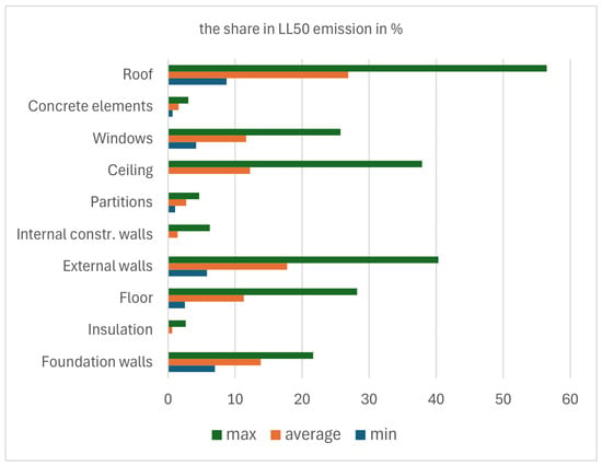
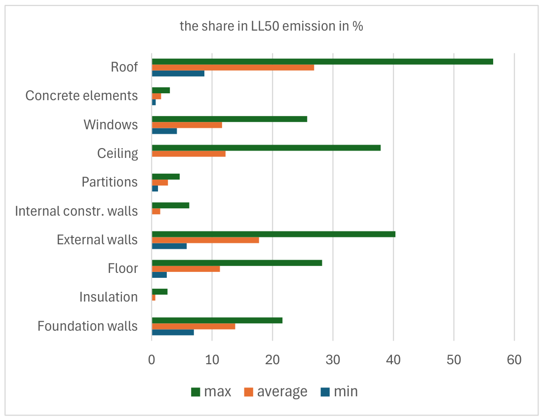
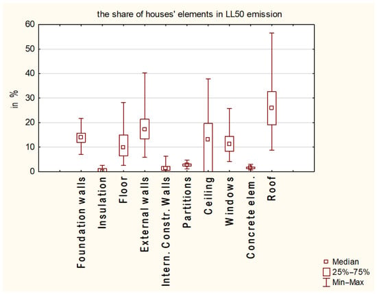
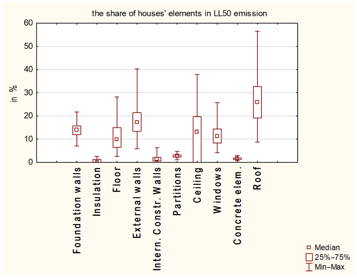
As presented in Section 2 of this article, 10 elements of a house are considered in calculating LL50 emission for each house. Table 9 presents the descriptive statistics for these elements.

Table 9. Descriptive statistics of LL50 emissions for particular house elements.

Sample	Number of Types of Houses’ Structures	Mean	Minimum	Maximum	Standard Deviation
Foundation walls	11,907	13.8366	6.9948	21.6458	2.705626
Insulation	11,907	0.6144	0.0000	2.6299	0.698718
Floor	11,907	11.3079	2.5110	28.2047	5.965349
External walls	11,907	17.7663	5.8111	40.3339	5.776132
Internal constr. walls	11,907	1.4251	0.0000	6.2379	1.073772
Partitions	11,907	2.6994	1.0526	4.6500	0.601224
Ceiling	11,907	12.2345	0.0000	37.8934	9.829270
Windows	11,907	11.6588	4.1840	25.7409	4.191249
Concrete elements	11,907	1.5719	0.6833	3.0268	0.398152
Roof	11,907	26.8850	8.7322	56.4928	9.640634

The strength of the variations in the shares is presented in Figure 6 and Figure 7.

Figure 6. Min–average–max share of house elements in LL50 emission.

Figure 7. The box plots of the distribution of house elements in LL50 emission.

3.4. The Ranking of the Houses’ Features Based on Their Influence on the LL50 Emission

To assess the importance of the selected features for the value of LL50 emission, decision trees are used. We assigned a class to each of the 11,907 house structure types. If the value of LL50 for a given case is lower than the median value, the class assigned is Low (L). If not, the assigned class is High (H). Before running the software to search for the best classifying decision tree, the variables are set:

• Dependent variable, i.e., the class (H or L);
• Independent variables:

  -

  Area of a house (named Area);

  -

  Type of a house according to the number of storeys (Storey);

  -

  Type of roof shape (Roof);

  -

  Type of complexity of the building’s shape (Shape);

  -

  Type of construction material for the external walls (External walls_m);

  -

  Type of construction material for the internal walls (Internal walls_m);

  -

  Type of construction material for the partitions (Partitions_m);

  -

  Type of construction material for the ceiling (Ceiling_m);

  -

  Type of construction material for the foundation (Foundation_m).

(The m letter added to the names of the independent variables indicates that the choice refers to the type of construction materials.)

The split is allowed over 200 cases in a node, and the maximum number of nodes is defined as 1000. As there is a large number of cases (11,907), the cases were randomly split into the training and testing subsets. For the same reason, it is not necessary to apply a cross-validation procedure. Of the total number of cases, 15% were assigned to the testing subset. The aim of DT application is not to predict a class or a number but just to find the importance ranking of the independent variables. The result of this automated classification by the DT found by the software, i.e., the confusion matrix, is presented in Table 10.

Table 10. The confusion matrix for classifying all 11,907 types of houses’ structures to the Low and High classes of LL50 emission.

	Class Predicted: Low	Class Predicted: High	Total Number of Cases in the Observed Class
Observed class Low	5663	291	5954
Observed class High	330	5623	5953

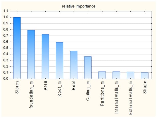
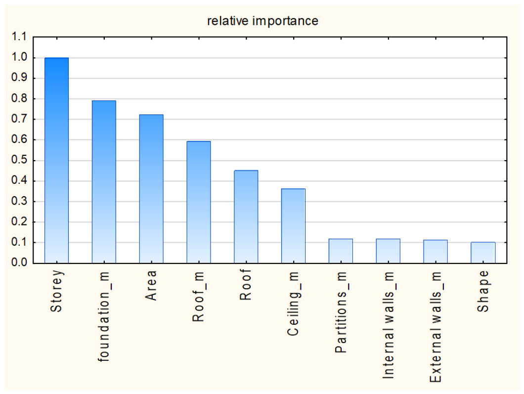
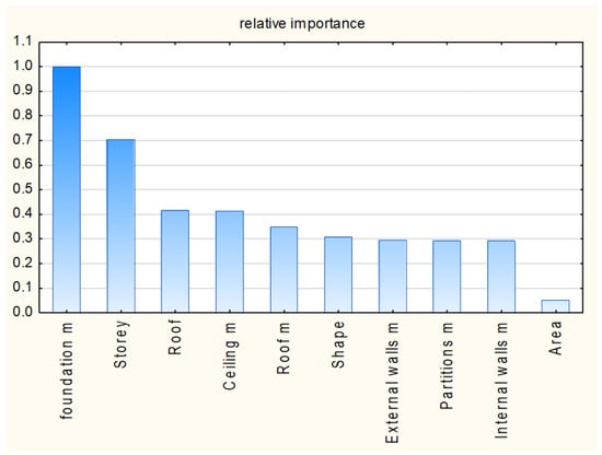
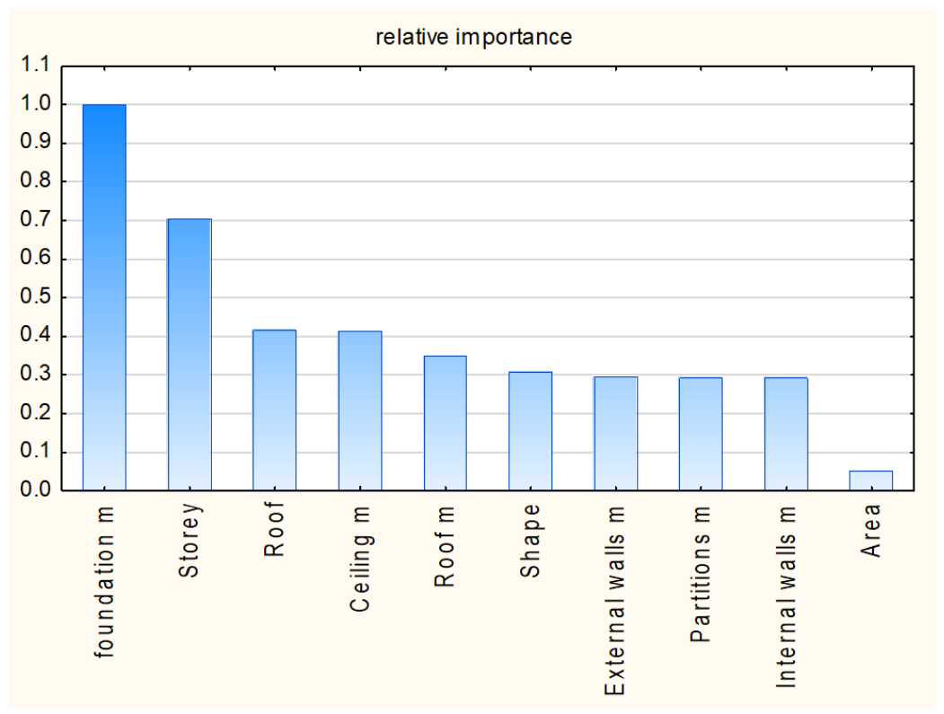
The overall accuracy achieved is 94.8%. Knowing that, the ranking of features (independent variables) presented below in Table 11 and in Figure 8 can be assessed as meaningful.

Table 11. The ranking of importance of features (independent variables) for the classification to Low and High classes of LL50 (for all types of the houses’ structures).

Feature	Rank	Importance
Storey	100	1.000000
Foundation_m	79	0.793255
Area	73	0.725378
Roof_m	59	0.593249
Roof	45	0.451064
Ceiling_m	36	0.363528
Partitions_m	12	0.120100
Internal walls_m	12	0.120100
External walls_m	11	0.114245
Shape	10	0.103232

Figure 8. The relative importance of features (independent variables) for the classification to Low and High classes of LL50 (for all types of houses’ structures).

Because the drivers of embodied emissions may differ fundamentally between standard and large-scale residential buildings, the dataset is divided into two contrasting subsets. The first subset encompasses houses with an area up to 150 sqm (6615 cases), representing typical, economical single-family housing. The second subset includes houses with an area of 180 sqm and above (5292 cases), representing large or premium residential properties. The intermediate area (between 150 and 180 sqm) was intentionally omitted from this specific classification step to establish a clear boundary and polarize the two groups. This methodological choice sharpens the contrast between the datasets, ensuring the classification tree’s feature importance reflects distinct structural and architectural typologies rather than transitional cases. The procedure of creating the DT classifier and ranking feature importance is repeated for these two subsets. The confusion matrix for the subset comprising lower houses (i.e., 40 to 150 sqm) is presented in Table 12.

Table 12. The confusion matrix for classifying all 11907 types of houses’ structures to the Low and High classes of LL50 emission (for houses of the lower area).

	Class Predicted: Low	Class Predicted: High	Total Number of Cases in the Observed Class
Observed class Low	5449	114	5563
Observed class High	96	956	1052

The overall accuracy achieved is 96.8%. However, the minimum split is set at 50 cases in a node this time. Knowing that, the ranking of features (independent variables) presented below in Table 13 and in Figure 9 can be assessed as meaningful.

Table 13. The ranking of importance of features (independent variables) for the classification to Low and High classes of LL50 (for houses of the lower area).

Feature	Rank	Importance
Foundation m	100	1.000000
Storey	71	0.705124
Roof	42	0.416130
Ceiling_m	41	0.413694
Roof_m	35	0.350479
Shape	31	0.307773
External walls_m	30	0.295966
Partitions_m	29	0.292482
Internal walls_m	29	0.292482
Area	5	0.052096

Figure 9. The relative importance of features (independent variables) for the classification to Low and High classes of LL50 (for houses of the lower area).

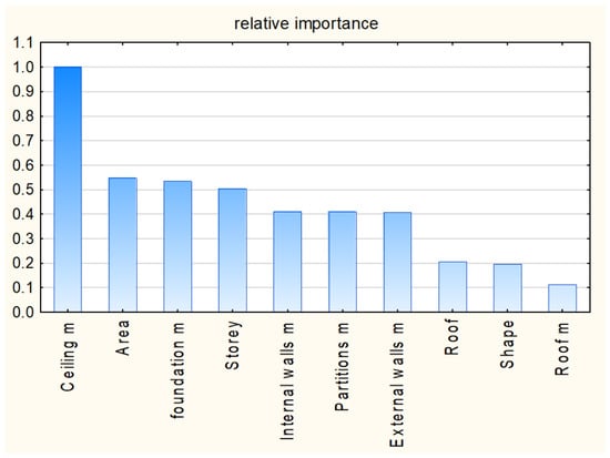
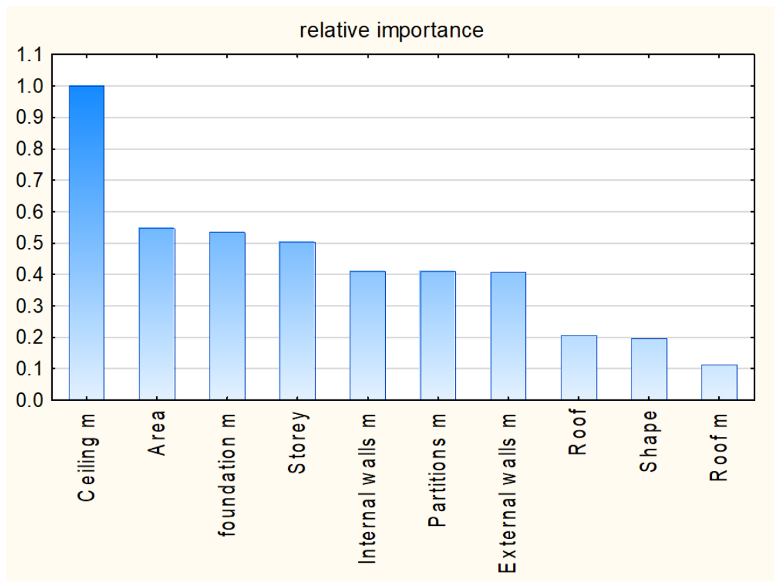
The third attempt at classification by the DT is based on 5292 types of houses’ structures where the area of the houses is from 180 to 300 sqm. Here, the split limit is set to 50 cases in the node. The confusion matrix is presented in Table 14.

Table 14. The confusion matrix for classifying all 11907 types of houses’ structures into the Low and High classes of LL50 emission (for houses of the higher area).

	Class Predicted: Low	Class Predicted: High	Total Number of Cases in the Observed Class
Observed class Low	310	81	391
Observed class High	38	4863	4901

The overall accuracy achieved is 97.8%. Considering that, the ranking of features (independent variables) presented below in Table 15 and Figure 10 can be assessed as meaningful.

Table 15. The ranking of importance of features (independent variables) for the classification to Low and High classes of LL50 (for houses of the higher area).

Feature	Rank	Importance
Ceiling_m	100	1.000000
Area	55	0.546360
Foundation_m	53	0.534446
Storey	50	0.503162
Internal walls_m	41	0.410694
Partitions_m	41	0.410694
External walls_m	41	0.406561
Roof	21	0.205858
Shape	20	0.196638
Roof_m	11	0.112460

Figure 10. The relative importance of features (independent variables) for the classification to Low and High classes of LL50 (for houses of the higher area).

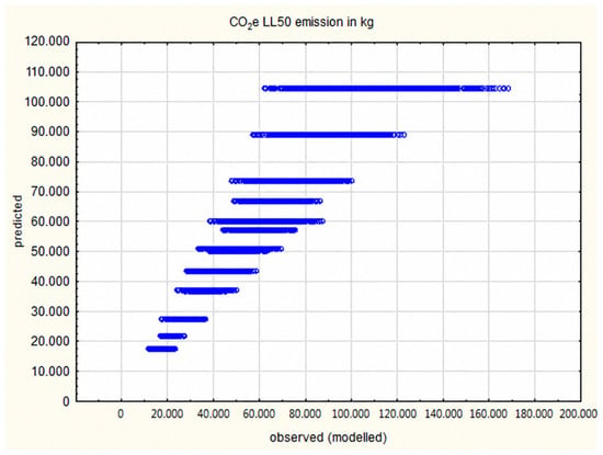
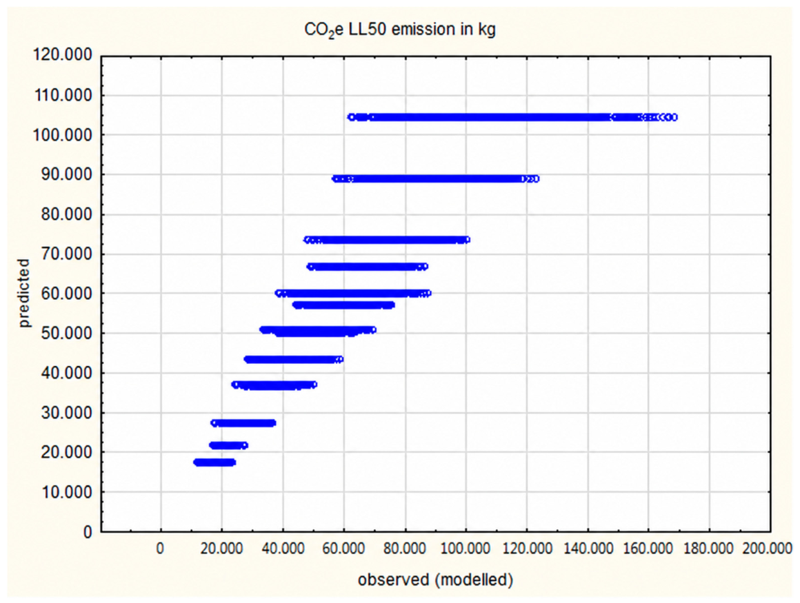
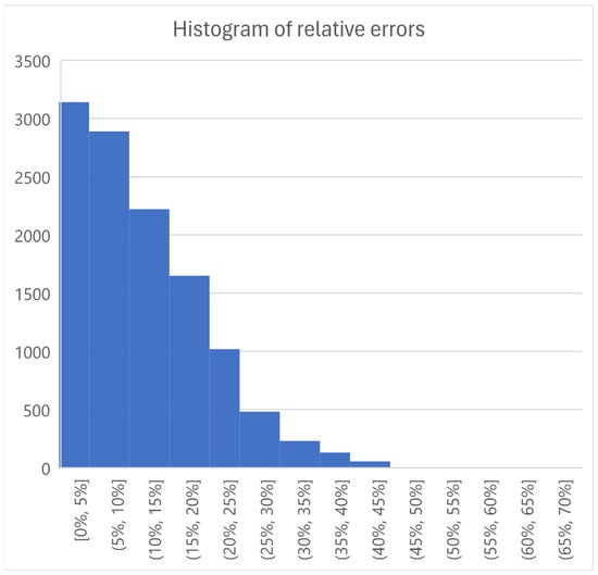
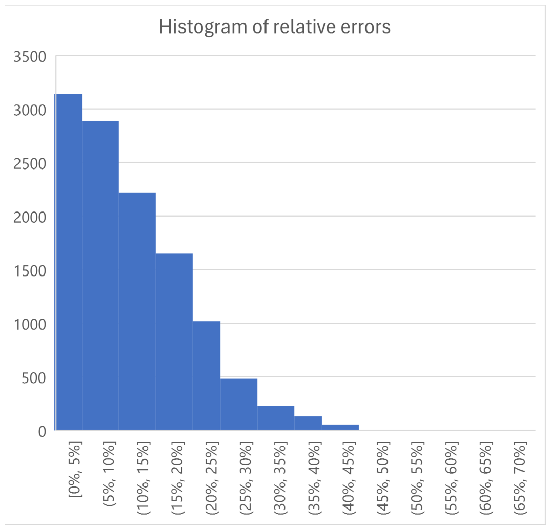
The attempt to assess the feature importance through predicting the LL50 values by the decision trees has failed (see Figure 11, where predicted values are presented vs. original values). Despite the mean absolute percentage error (mean relative error) being promising, i.e., 11.7%, the distribution of errors, presented in Figure 12, shows that over 50% of cases have an absolute relative error higher than 10% (reaching 55.6% maximum).

Figure 11. LL50 emissions observed vs. predicted.

Figure 12. The histogram of absolute relative prediction errors.

Moreover, the house area is the only numerical independent variable. The remaining independent variables are categorical, so naturally it is found to be the most important predictor. For these reasons, it was decided to base the reasoning about predictors’ importance on the classifications.

4. Discussion

4.1. The Predictive Importance of Construction Materials vs. Geometric Properties on CO₂e Classification

Based on the rankings of properties influencing the lifelong CO₂e emission presented in Figure 8, Figure 9 and Figure 10, it is possible to compare the influence of the construction materials used for the houses’ structures and the properties related to the shape of the houses. To do so, the relative importance of the influence presented in Table 9, Table 11 and Table 13 are transformed to values whose sums are equal to 1 for each table. The result is presented in Table 16.

Table 16. The relative importance of features for houses of the higher area and lower area on LL50.

Feature	Importance for Houses of Higher Area	Importance for Houses of Lower Area
Ceiling_m	0.2311	0.1003
Area	0.1263	0.0126
Foundation_m	0.1235	0.2424
Storey	0.1163	0.1709
Internal walls_m	0.0949	0.0709
Partitions_m	0.0949	0.0709
External walls_m	0.0940	0.0717
Roof	0.0476	0.1009
Shape	0.0454	0.0746
Roof_m	0.0260	0.0849
SUM	1.0000	1.0000

It is possible to calculate the total influence of construction materials (properties with the mark m at the end of the description) and the influence of non-material house properties. Table 17 presents the results.

Table 17. The relative importance of construction materials and non-material features of houses for houses of the higher area and lower area on LL50.

Feature	Importance for Houses of Higher Area	Importance for Houses of Lower Area
Construction materials	0.6644	0.6410
Non-material features of houses	0.3356	0.3590
SUM	1.0000	1.0000

Despite the differences observed in Table 17, it is evident that non-material properties (i.e., area of the house, number of storeys, roof shape, and building shape) hold a substantial relative importance in the C&RT models—accounting for approximately 33.6% of the model’s predictive power for larger houses and 35.9% for smaller houses. However, it must be strongly emphasized that these values represent model-based feature importance (i.e., the variables’ relative contribution to improving node purity in the classification tree algorithm) and should not be interpreted directly as a causal decomposition of the physical embodied emissions. They indicate how effectively a given feature classifies the LL50 emission level within the model, not the absolute percentage of CO₂e kilograms attributed to that feature.

Nevertheless, this high predictive importance robustly demonstrates that non-material design parameters are dominant drivers of the final carbon classification. This is a critical observation, emphasizing that clients—who are usually non-professionals concerned more with the size, shape, and visual appeal of the house than with specific construction materials—inadvertently make early-stage decisions that strongly dictate the building’s overall sustainability profile.

Another important finding is that, based on the results presented in Table 17, it can be stated that the influence of the area of the building is 10 times higher for the houses of higher area than for houses of lower area.

4.2. The Influence of the Area of the House on U50 and LL50 Emissions

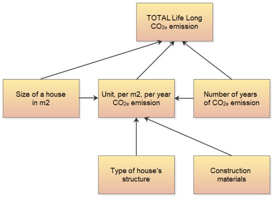
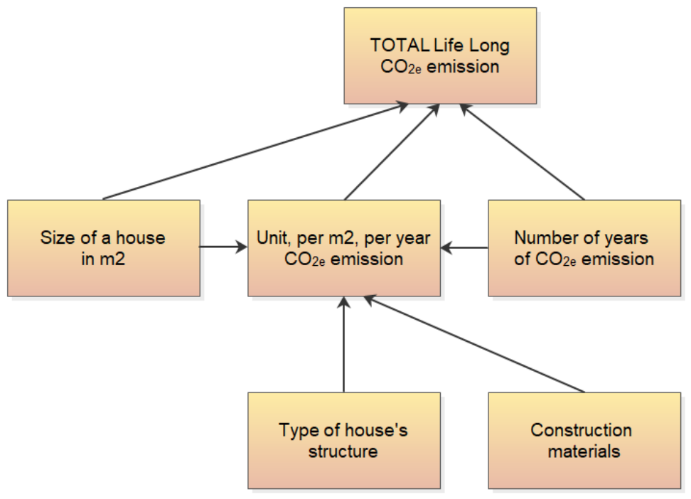
The unit, i.e., per square meter, emission is a function of the two groups of parameters:

-

Types of construction materials used for erecting a house;

-

Type of a house structure, which is non-construction materials features of a house, and the house area, and the number of years (see Figure 13).

Figure 13. The groups of factors (or the single factors) influencing unit U50 and life-long LL50 CO₂e embodied emissions.

As can be observed in Figure 5, the bigger the house area, the lower U50. The statistical importance of the differences between the groups of houses of different areas is proven. However, the bigger the house area, the bigger the life-long LL50 emission. As can be observed in Figure 4, this relationship—also statistically confirmed—is much stronger than in the case of U50 emissions.

The LL50 emission depends on unit emission, the number of years (50 in this case), and the area of a house. Introducing regulations that limit only the unit emission might create an unintended regulatory incentive. Because it is mathematically easier to achieve a lower U50 in a larger house, such rules could inadvertently encourage the design of larger buildings just to meet the threshold. As a consequence, the total (life-long) emission LL50 would be much higher, as the relationship between a house area and LL50 is significantly stronger than the relationship between a house area and the unit emission U50. However, since actual investor or household behavior is not modeled in this study, this remains a potential unintended consequence requiring further multidisciplinary investigation.

4.3. Design Scenario Feasibility Considering LL50 and U50 Limits

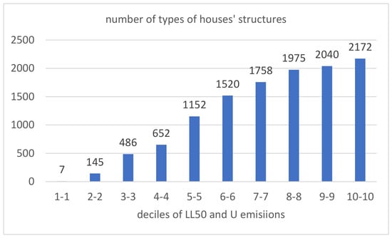
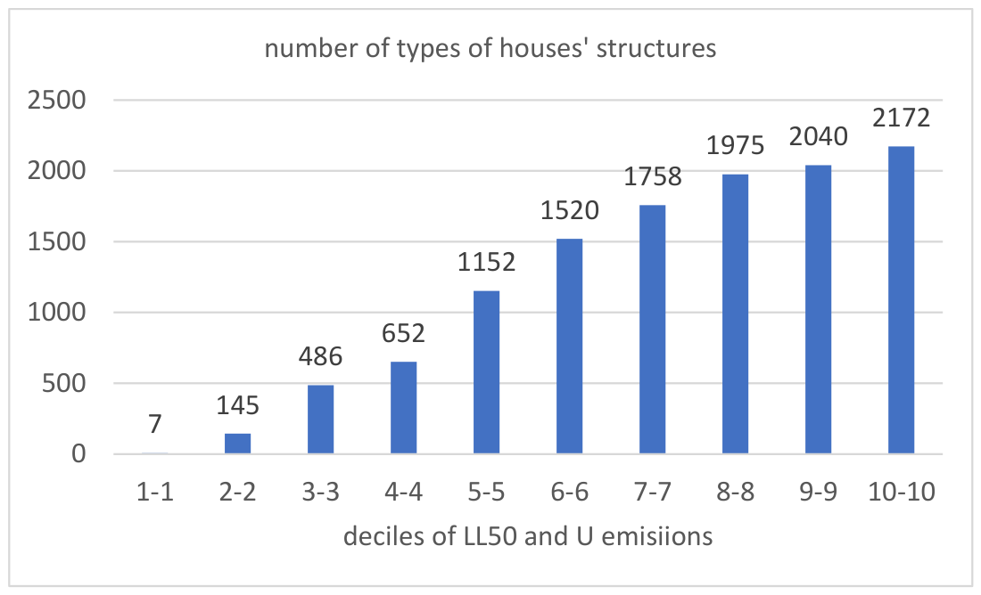
Limiting both LL50 and U50 emissions simultaneously could severely restrict the available design scenarios, making it difficult or even impossible to find a feasible material and structural combination if the emission limits are set too low. The database that refers to the 50-year life cycle of the building has been filtered several times to find the houses’ structures whose LL50 emission and U50 emission are in the same decile. The number of houses’ structures meeting these criteria is presented in Figure 14.

Figure 14. The number of the houses’ structures that belongs simultaneously to the same decile of LL50 and U50 emissions.

5. Conclusions

Data available today are not complex, which does not allow for pointing out the best materials for sustainable buildings. In theory, data based on EPDs should be reliable, as they are based on international standards and are subject to third-party verification. In fact, comparing EPDs of the same type of material often leads to entirely different conclusions. This is the reason why many parties have been waiting for harmonized standards adaptation to the newly adopted CPR regulation (Regulation (EU) 2024/3110) [13]. After the new CPR is fully implemented, CO₂e footprint is going to be declared in the Declaration of Performance and Conformity, and manufacturers will take more responsibility for declared values. The implementation will last at least a few years.

LCA analysis should include the embodied footprint in the whole life cycle. At the moment, it depends on the EU members whose modules are taken in the calculation [61]; thus, buildings are evaluated differently. It is essential to take all modules for calculation and compare the same data, as it has a huge impact on the overall analysis. The initial evaluation of A1 to A3 modules may be misleading, as, e.g., recarbonation [62] during the use phase and the required replacement of non-durable layers may significantly change the evaluation of materials. The end-of-life phase of the material is also important for the complexity of the LCA analysis.

Although the C&RT analysis demonstrates that the choice of construction materials holds the highest predictive weight for total embodied emissions (accounting for approximately 64–66% of the aggregated feature importance), non-material parameters—such as floor area, number of storeys, roof type, and building shape—still account for a substantial portion of the predictive model (over 34%). While material selection is the dominant factor, the architectural geometry determines the total surface area of the partitions, effectively acting as a multiplier for the material-related emissions. Therefore, building shape and size optimization remains a crucial early-stage design strategy. It provides an objective basis for reducing absolute emissions before specific material decisions are finalized, which is especially valuable when environmental data for construction products is still uncertain.

Any regulation in countries should not focus solely on emissions per 1 square meter, because, as proven in this study, the larger the house is, the lower the GWP per m². In the case of limits based strictly on the unit of living area, it is mathematically easier to meet the threshold by building a larger house rather than a smaller one. This creates a potential unintended regulatory incentive that might inadvertently encourage the construction of larger buildings, which is not sustainable when total absolute emissions are concerned.

The highest emissions from the roof result from the membranes used; choosing different materials can change their share in total emissions. The factor that has the strongest influence is the material of the ceiling. On the one hand, the ceiling is the building component with a high CO₂e footprint, and it was expected that the share in CO₂e footprint would be the highest. The second fact is that the ceiling can have an area that can be equal to the area of the building (bungalow with sloping roof), or a ceiling may not even exist (bungalow with flat roof).

The second factor that has the strongest influence is the area of the building, as comparing the two opposite areas, 40 and 300 m², in the case of the rectangular shape of the bungalow building with a flat roof, one has a circumference-to-area ratio of 0,6, while the second has a ratio of 7.50.

Many variables in total embodied emissions can influence the result. Factors that are to be optimized depend on building type. Data consistency must be ensured before performing optimization, which will probably only be possible after introducing responsibility for declaring environmental parameters.

Despite the significant findings, this study has several limitations that should be acknowledged. First, the database of construction materials and their structural combinations is based primarily on the Polish market and national thermal requirements. Consequently, the results and the exact shares of embodied emissions may vary for other climates and regions with different construction practices. Second, the environmental product declarations (EPDs) currently available do not cover all products on the market, and data consistency is still developing. Third, it should be pointed out that the database refers to a specific set of buildings. Thus, it provides only an approximation of the partitions’ areas and their CO₂e footprints. Every building is individual, so these general results cannot be directly applied to any specific design situation. Due to these facts, the obtained calculations should be treated as estimates only. Furthermore, because module B4 (replacement) strongly contributes to the differences between the 50-, 70-, and 100-year scenarios, the precise rankings of material importance generated by the C&RT analysis are sensitive to the assumed service lives and EPD selection. Modifying the replacement cycles for key components or choosing different EPD sources could shift the relative importance of specific materials. Finally, the analysis is limited strictly to single-family houses. Future research should expand the database to include multi-family residential and commercial buildings, as well as incorporate a wider range of European markets to verify the broader applicability of the presented conclusions.

References

- European Commission. Improving Energy Efficiency of Buildings to Reduce Bills and Save Energy. 29 May 2026. Available online: https://commission.europa.eu/news-and-media/news/improving-energy-efficiency-buildings-reduce-bills-and-save-energy-2026-05-29_en (accessed on 8 October 2026).
- Eurostat. Renewables Make Up 26% of EU Energy Use. 23 July 2026. Available online: https://ec.europa.eu/eurostat/web/products-eurostat-news/w/ddn-20260723-1 (accessed on 8 October 2026).
- Cabeza, L.F.; Barreneche, C.; Miró, L.; Morera, J.M.; Bartolí, E.; Fernández, A.I. Low carbon and low embodied energy materials in buildings: A review. Renew. Sustain. Energy Rev. 2013, 23, 536–542. [Google Scholar] [CrossRef] [Scilit]
- Directive (EU) 2024/1275 of the European Parliament and of the Council of 24 April 2024 on the Energy Performance of Buildings (Recast). Available online: https://eur-lex.europa.eu/eli/dir/2024/1275/oj (accessed on 8 October 2026).
- Khan, S.; Alam, T.; Khan, M.; Blecich, P.; Kamal, M.; Gupta, N.; Yadav, A. Life Cycle Assessment of Embodied Carbon in Buildings: Background, Approaches and Advancements. Buildings 2022, 12, 1944. [Google Scholar] [CrossRef] [Scilit]
- Cabeza, L.F.; Boquera, L.; Chàfer, M.; Vérez, D. Embodied energy and embodied carbon of structural building materials: Worldwide progress and barriers through literature map analysis. Energy Build. 2021, 231, 110612. [Google Scholar] [CrossRef] [Scilit]
- Tirelli, D.; Besana, D. Moving toward Net Zero Carbon Buildings to Face Global Warming: A Narrative Review. Buildings 2023, 13, 684. [Google Scholar] [CrossRef] [Scilit]
- Arenas, N.F.; Shafique, M. Reducing embodied carbon emissions of buildings—A key consideration to meet the net zero target. Sustain. Futures 2024, 7, 100166. [Google Scholar] [CrossRef] [Scilit]
- Guidetti, E.; Ferrara, M. Embodied energy in existing buildings as a tool for sustainable intervention on urban heritage. Sustain. Cities Soc. 2023, 88, 104284. [Google Scholar] [CrossRef] [Scilit]
- Zhang, J.; Yuan, J.; Su, S.; Zhou, S.; Hao, J.; Fang, Q. Predicting the operational carbon emissions of urban community service units by using a two-stage explainable machine learning method: A case study in Nanjing, China. J. Asian Archit. Build. Eng. 2025, 1–16. [Google Scholar] [CrossRef] [Scilit]
- Fenton, S.K.; Munteanu, A.; De Rycke, K.; De Laet, L. Embodied greenhouse gas emissions of buildings—Machine learning approach for early stage prediction. Build. Environ. 2024, 257, 111523. [Google Scholar] [CrossRef] [Scilit]
- Su, S.; Zang, Z.; Yuan, J.; Pan, X.; Shan, M. Considering critical building materials for embodied carbon emissions in buildings: A machine learning-based prediction model and tool. Case Stud. Constr. Mater. 2024, 20, e02887. [Google Scholar] [CrossRef] [Scilit]
- Regulation (EU) 2024/3110 of the European Parliament and of the Council of 27 November 2024 Laying Down Harmonised Rules for the Marketing of Construction Products and Repealing Regulation (EU) No 305/2011. Available online: https://eur-lex.europa.eu/eli/reg/2024/3110/oj (accessed on 27 October 2026).
- Tozan, B.; Hoxha, E.; Brisson Stapel, E.; Birgisdottir, H. Prioritizing low-carbon materials and reducing material quantities to mitigate embodied GHG emissions in buildings. Sustain. Cities Soc. 2025, 131, 106770. [Google Scholar] [CrossRef] [Scilit]
- Szalay, Z. A parametric approach for developing embodied environmental benchmark values for buildings. Int. J. Life Cycle Assess. 2024, 29, 1563–1581. [Google Scholar] [CrossRef] [Scilit]
- Jungclaus, M.A.; Grant, N.; Torres, M.I.; Arehart, J.H.; Srubar, W.V., III. Embodied carbon benchmarks of single-family residential buildings in the United States. Sustain. Cities Soc. 2024, 117, 105975. [Google Scholar] [CrossRef] [Scilit]
- Rabenseifer, R.; Provazník, R.; Mahas, N.; Minarovičová, K.; Jamnický, M.; Ždímalová, M.; Khrapatova, I.; Semko, V. Simplified Product-Stage LCA of Family Houses: The Role of Geometry, Proportions, and Size. Energies 2026, 19, 161. [Google Scholar] [CrossRef] [Scilit]
- Budownictwo w 2023 Roku. Available online: https://stat.gov.pl/obszary-tematyczne/przemysl-budownictwo-srodki-trwale/budownictwo/budownictwo-w-2023-roku,13,21.html (accessed on 3 June 2024).
- Produkcja Wyrobów Przemysłowych w 2022 Roku. Available online: https://stat.gov.pl/obszary-tematyczne/przemysl-budownictwo-srodki-trwale/przemysl/produkcja-wyrobow-przemyslowych-w-2022-roku,3,20.html (accessed on 3 June 2024).
- Kalkulator Budowlany. Available online: https://kalkulatorbudowlany.ytong-silka.pl/index.php?task=calculator&action=prepareCalculationData (accessed on 7 June 2024).
- Dz.U.2022.0.1225 t.j.-Rozporządzenie Ministra Infrastruktury z Dnia 12 Kwietnia 2002 r. w Sprawie Warunków Technicznych, Jakim Powinny Odpowiadać Budynki i Ich Usytuowanie. Available online: https://eli.gov.pl/eli/DU/2002/690/ogl (accessed on 27 October 2026).
- Available online: https://www.nachhaltigesbauen.de/fileadmin/pdf/baustoff_gebauededaten/BNB_Nutzungsdauern_von_Bauteilen_2017-02-24.pdf (accessed on 1 June 2024).
- Available online: https://www.eco-platform.org/epd-data.html (accessed on 3 June 2024).
- Available online: https://www.environdec.com/pcr-library (accessed on 3 June 2024).
- Available online: https://www.oekobaudat.de/ (accessed on 3 June 2024).
- PN-EN 1990:2004; Eurokod—Podstawy Projektowania Konstrukcji. Polski Komitet Normalizacyjny: Warsaw, Poland, 2004.
- Available online: https://www.rp.pl/nieruchomosci/art37737731-milion-mieszkan-w-polsce-ma-ponad-100-lat (accessed on 10 June 2024).
- EN 15804:2012+A1:2013; Sustainability of Construction Works-Environmental Product Declarations-Core Rules for the Product Category of Construction Products. European Committee for Standardization (CEN): Brussels, Belgium, 2013.
- EN 15804:2012+A2:2019; Sustainability of Construction Works-Environmental Product Declarations-Core Rules for the Product Category of Construction Products. European Committee for Standardization (CEN): Brussels, Belgium, 2019.
- Fisher, R.A. The Correlation Between Relatives on the Supposition of Mendelian Inheritance. Philos. Trans. R. Soc. Edinb. 1918, 52, 399–433. [Google Scholar] [CrossRef] [Scilit]
- Safari, M.; Abtahi, S.M.; Joudaki, J. Experimental Modeling, Statistical Analysis, and Optimization of the Laser-Cutting Process of Hardox 400 Steel. Materials 2024, 17, 2798. [Google Scholar] [CrossRef] [Scilit]
- Negovetic Mandic, V.; Plancak, L.; Marovic, D.; Tarle, Z.; Trutina Gavran, M.; Par, M. Mechanical Properties of Alkasite Material with Different Curing Modes and Simulated Aging Conditions. Materials 2024, 17, 2777. [Google Scholar] [CrossRef] [Scilit]
- Pop, A.B.; Titu, A.M.; Ravai-Nagy, S.; Daraba, C. Influence of Machining Parameters on the Dimensional Accuracy of Drilled Holes in Engineering Plastics. Polymers 2024, 16, 1490. [Google Scholar] [CrossRef] [Scilit]
- Jakubowski, J.; Kot, S.M.; Sokołowski, J. Statystyka, 2nd ed.; Difin: Warsaw, Poland, 2011. [Google Scholar]
- Józefacka, N.; Arciszewska-Leszczuk, A.; Kołek, F.M.; Iwankowski, P. Metodologia i Statystyka. Przewodnik Naukowego Turysty. Tom 1; PWN: Warsaw, Poland, 2023. [Google Scholar]
- Aczel, A.D. Statystyka w Zarządzaniu, 2nd ed.; PWN: Warsaw, Poland, 2022. [Google Scholar]
- Rabiej, M. Statystyka z Programem Statistica; Helion: Gliwice, Poland, 2012. [Google Scholar]
- Shapiro, S.S.; Wilk, M.B. An analysis of variance test for normality (complete samples). Biometrika 1965, 52, 591–611. [Google Scholar] [CrossRef] [Scilit]
- Rees, G.; Hebryn-Baidy, L.; Belenok, V. Temporal Variations in Land Surface Temperature within an Urban Ecosystem: A Comprehensive Assessment of Land Use and Land Cover Change in Kharkiv, Ukraine. Remote Sens. 2024, 16, 1637. [Google Scholar] [CrossRef] [Scilit]
- Irzmańska, E.; Mizera, K.; Litwicka, N.; Sałasińska, K. An Approach to Testing Antivandal Composite Materials as a Function of Their Thickness and Striker Shape—A Case Study. Polymers 2024, 16, 591. [Google Scholar] [CrossRef] [Scilit]
- Levene, H. Robust tests for equality of variances. In Contributions to Probability and Statistics: Essays in Honor of Harold Hotelling; Olkin, I., Ghurye, S.G., Hoeffding, W., Madow, W.G., Mann, H.B., Eds.; Stanford University Press: Palo Alto, CA, USA, 1960; pp. 278–292. [Google Scholar]
- Gastwirth, J.L.; Gel, Y.R.; Miao, W. The Impact of Levene’s Test of Equality of Variances on Statistical Theory and Practice. Stat. Sci. 2009, 24, 343–360. [Google Scholar] [CrossRef] [Scilit]
- Nordstokke, D.W.; Zumbo, B.D. A Cautionary Tale About Levene’s Tests for Equal Variances. J. Educ. Res. Policy Stud. 2007, 7, 1–14. [Google Scholar]
- Cakir, E.; Duman, A.N.; Yildirim, A.Z.; Cevik, P. Shear Bond Strength between Orthodontic Brackets and Monolithic 4Y-TZP: An In Vitro Study. Materials 2023, 16, 5173. [Google Scholar] [CrossRef] [Scilit]
- Ferreiro-Seoane, F.J.; Miguéns-Refojo, V.; Atrio-Lema, Y. Can Talent Management Improve Training, Sustainability and Excellence in the Labor Market? Sustainability 2021, 13, 6645. [Google Scholar] [CrossRef] [Scilit]
- Kruskal, W.H.; Wallis, W.A. Use of ranks in one-criterion variance analysis. J. Am. Stat. Assoc. 1952, 47, 583–621. [Google Scholar] [CrossRef]
- Mann, H.B.; Whitney, D.R. On a Test of Whether one of Two Random Variables is Stochastically Larger than the Other. Ann. Math. Stat. 1947, 18, 50–60. [Google Scholar] [CrossRef] [Scilit]
- Kata, R.; Cyrek, M.; Wosiek, M. The Significance of the Financial Situation of Local Government Units for Their Energy Transition Activities: The Case of the Podkarpackie Region. Energies 2024, 17, 2761. [Google Scholar] [CrossRef] [Scilit]
- Mandičák, T.; Spišáková, M.; Mésároš, P. Sustainable Design and Building Information Modeling of Construction Project Management towards a Circular Economy. Sustainability 2024, 16, 4376. [Google Scholar] [CrossRef] [Scilit]
- Breiman, L.; Friedman, J.; Stone, C.J.; Olshen, R.A. Classification and Regression Trees; CRC Press: Boca Raton, FL, USA, 1984. [Google Scholar]
- Genuer, R.; Poggi, J.-M.; Tuleau-Malot, C. Variable selection using random forests. Pattern Recognit. Lett. 2010, 31, 2225–2236. [Google Scholar] [CrossRef] [Scilit]
- Strobl, C.; Boulesteix, A.-L.; Zeileis, A.; Hothorn, T. Bias in random forest variable importance measures: Illustrations, sources and a solution. BMC Bioinform. 2007, 8, 25. [Google Scholar] [CrossRef] [Scilit]
- Ishwaran, H. Variable importance in binary regression trees and forests. Electron. J. Stat. 2007, 1, 519–537. [Google Scholar] [CrossRef] [Scilit]
- Internetowy Podręcznik Statystyki. Available online: https://www.statsoft.pl/textbook/stathome.html (accessed on 5 June 2024).
- Anysz, H.; Brzozowski, Ł.; Kretowicz, W.; Narloch, P. Feature Importance of Stabilised Rammed Earth Components Affecting the Compressive Strength Calculated with Explainable Artificial Intelligence Tools. Materials 2020, 13, 2317. [Google Scholar] [CrossRef] [Scilit]
- Anysz, H.; Dąbrowska, M. The Risk Indicators of Construction Projects’ Cost Overruns Assessed with PCA, Decision Trees, and Pearson’s Correlations. In XXX Russian-Polish-Slovak Seminar Theoretical Foundation of Civil Engineering (RSP 2021); Akimov, P., Vatin, N., Eds.; Lecture Notes in Civil Engineering; Springer: Cham, Switzerland, 2022; Volume 189, pp. 424–432. [Google Scholar] [CrossRef] [Scilit]
- Dunn, O.J. Multiple Comparisons Using Rank Sums. Technometrics 1964, 6, 241–252. [Google Scholar] [CrossRef]
- Dinno, A. Nonparametric pairwise multiple comparisons in independent groups using Dunn’s test. Stata J. 2015, 15, 292–300. [Google Scholar] [CrossRef] [Scilit]
- Holm, S. A Simple Sequentially Rejective Multiple Test Procedure. Scand. J. Stat. 1979, 6, 65–70. [Google Scholar]
- Cliff, N. Dominance statistics: Ordinal analyses to answer ordinal questions. Psychol. Bull. 1993, 114, 494–509. [Google Scholar] [CrossRef]
- Available online: https://worldgbc.org/wp-content/uploads/2023/03/1744-WGBC-Position-Paper-FINAL-200323.pdf (accessed on 22 November 2024).
- Walther, H. Recarbonation matters—CO2 absorption of AAC during its use phase. ce/papers 2023, 6, 246–251. [Google Scholar] [CrossRef] [Scilit]
- Rogala, W. Embodied Emissions for Different Type of Single-Family Houses; Mendeley Data: Amsterdam, The Netherlands, 2024; Version 1. [Google Scholar] [CrossRef]
Disclaimer/Publisher’s Note: The statements, opinions and data contained in all publications are solely those of the individual author(s) and contributor(s) and not of MDPI and/or the editor(s). MDPI and/or the editor(s) disclaim responsibility for any injury to people or property resulting from any ideas, methods, instructions or products referred to in the content. |
© 2026 by the authors. Licensee MDPI, Basel, Switzerland. This article is an open access article distributed under the terms and conditions of the Creative Commons Attribution (CC BY) license.