PySkyLumos: A Python-Based Polarized Skylight Simulator

Abstract

This paper presents PySkyLumos, an open-source Python framework for simulating skylight polarization measurements and metadata. It implements the Rayleigh, Berry, and Pan models, covering single scattering, the splitting of the neutral points caused by multiple scattering, and the elevation-dependent motion of these points. Benchmarks show a fivefold overall speed-up and up to two orders of magnitude faster Stokes-parameter image formation than a recent open-source simulator. Validation against real polarization-camera images shows close agreement between the simulated and measured polarization patterns, supporting its use in algorithm development for bio-inspired computer vision, navigation, robotics, and sensing.

1. Introduction

Light is electromagnetic radiation that propagates as a transverse wave of mutually perpendicular electric and magnetic fields; the electric field’s oscillation defines the polarization state [1,2,3]. Sunlight is unpolarized before entering the atmosphere, but scattering by air molecules and aerosols generates characteristic polarized sky patterns [4,5,6,7]. It is difficult to establish when polarized light was first observed or used. Systematic optical studies are documented from Bartholin’s work on Icelandic spar in 1669 [1,2], but historical evidence suggests earlier use of polarization cues, such as Viking navigation with “sunstones” [2,3]. Polarization sensitivity is also widespread in the animal kingdom, enabling navigation, scene recognition, and communication [3,8,9,10,11,12]. Polarized light is now also used in measurement science, for example, in remote sensing [13,14], cloud reconstruction [15], navigation [16], material analysis and characterization [17], and even consumer products [18].

Recent studies combine polarization imaging with machine learning and deep learning methods [13,14,19]. Since humans cannot directly perceive the polarization state of light, dedicated sensors are required [20,21,22]. However, such sensors are often costly, and collecting sufficient measurements for algorithm training is time-consuming. To reduce this effort, several polarization image datasets [23,24] and simulators [24,25,26] have been released. Existing datasets, however, lack polarization-specific metadata, such as the astronomical positions of singularity points, and current simulators do not automatically provide the ability to generate datasets enriched with this information. Researchers must therefore build their own datasets and implement astronomical computations, such as frame transformations and Sun-position algorithms, before they can start their actual research. In addition, none of the available datasets or simulators includes a recently developed skylight polarization model, the Pan model [7].

To address these gaps, we have developed PySkyLumos [27,28], a self-contained Python toolkit for skylight-polarization simulation and sensor emulation. Unlike previous tools, it implements the state-of-the-art Pan model [7]; it runs faster than previous Python simulators through vectorized computation; and it outputs metadata such as the astronomical positions of the polarization singularities, which supports instrument development and bio-inspired perception.

The rest of the paper is organized as follows: Section 1.1 reviews related work; Section 2 describes the Rayleigh, Berry, and Pan models and details the PySkyLumos methodology and implementation; Section 3 reports benchmarks, comparisons to OpenSky, and validation against field measurements; and Section 4 discusses their implications and concludes with future directions.

1.1. Related Work

Existing simulators focus primarily on the Rayleigh and Berry models [4,5,6] and do not include the more recent Pan model [7], which extends the Berry model with neutral points whose positions depend on the solar elevation. This section summarizes these simulators and then outlines the improvements introduced by the present work.

1.1.1. Polarized Skylight Navigation Simulation Dataset (PSNS)

In [24], the authors constructed a polarized-skylight navigation dataset based on the Berry model [5,6] combined with the Hosek luminance model [29,30]. The dataset contains approximately 138,000 images recorded at analyzer orientations of 0°, 45°, 90°, and 135°, including both noise-free and noisy variants. It was generated using the hypothetical polarization camera described by prior work [25], together with an external Sun-position model. A Lucid Vision Labs polarization camera (Richmond, BC, Canada) [31] incorporating a Sony micro-polarizer array (Sony Semiconductor Solutions Corporation, Atsugi, Japan) [32] was used to inform the sensor model. Several sensor parameters are included, but noise characteristics and lens conjugation are not modeled explicitly. Neither the dataset nor the simulator provides polarization-specific metadata, such as the anti-Sun position or the astronomical locations of the singularity points. The associated C++ software is publicly available on GitHub [33,34], but this release implements only the Rayleigh sky model.

1.1.2. OpenSky

OpenSky [26] is the current state-of-the-art Python skylight-polarization simulator and also has a MATLAB implementation. It supports both the Rayleigh and Berry models, together with a photometric relative-radiance formulation, namely the CIE model [29,35,36,37,38]. Its modular design provides either the outputs of the physical models alone or the simulated outputs of a micro-polarizer imaging sensor, the Sony IMX250MZR [32]. Compared with [24,25], it also includes five optical models of the objective lens [39]. Like the other tools discussed in this paper, it does not provide polarization-specific metadata. OpenSky was validated by comparing simulated results with recordings from the Sony sensor and from standard cameras.

OpenSky is available on GitHub [40] for Python and MATLAB, together with a sample Jupyter Notebook. In the example, with the Sun at 0° altitude and 84° azimuth, the theoretical and sensor-model outputs are consistent, but for other Sun positions we found that the simulated sensor outputs depart from the theoretical predictions. In both versions of the public code (commit 62c52f4), the sensor simulation exchanges the positions of the 45° and 135° analyzers relative to the data-processing step, which reverses the sign of the recovered AOP; when the two positions are made consistent, the AOP recovered by OpenSky’s data processing agrees with OpenSky’s theoretical AOP to within approximately 0.2°. This minor inconsistency does not affect the physical models of OpenSky, whose outputs agree with those of PySkyLumos (Section 3.2).

1.1.3. Motivation for Current Work

Building on our analysis of existing simulators, PySkyLumos was designed to address several limitations found in the existing tools, thereby extending the applicability of skylight-polarization simulation. In particular, integrating a solar-ephemeris routine and automated reference-frame calculation eliminates the substantial pre-processing required in both PSNS [24,25] and OpenSky [26]. The PSNS framework [24,25,33,34], although centered on theoretical rendering, could be strengthened by extending its public code base beyond the Rayleigh implementation to include the Berry formulation, consistent with its dataset release. OpenSky [26], by contrast, would benefit from a mosaic-agnostic sensor layer, adoption of the Pan model [7], and fuller use of Python’s vectorized numerical libraries to improve throughput. Both platforms would also gain from incorporating polarization-specific metadata, such as singularity-point positions, as it enables more precise downstream analysis. Together, these enhancements would broaden the scientific utility of such tools while reducing barriers to their use.

2. Materials and Methods

2.1. Skylight Polarization Models

This section introduces the principal analytical models [4,5,6,7] of the skylight polarization distribution. The distribution of skylight polarization is determined primarily by the solar position [2,7,9,22,24,26]. Our study focuses on analytical rather than numerical formulations, because they are computationally efficient and give direct access to polarization-specific metadata. Although the Wilkie model [35] has seen wide use in computer graphics, it is excluded here because it cannot represent key physical features of skylight polarization, such as the neutral points, as noted by its authors [35]. The skylight polarization distribution is characterized by two parameters, the degree of polarization (DOP) and the angle of polarization (AOP). The DOP quantifies the fraction of light that is polarized, while the AOP specifies the orientation of the electric field’s vibration direction [1,2,3,4,5,6,7].

Throughout this paper, ${\theta }_p$ is the altitude (elevation above the horizon) of the observed sky point, ${\phi }_p=\pi /2-{\theta }_p$ its zenith angle, and ${\alpha }_p$ its azimuth, measured from North towards East; ${\theta }_s$, ${\phi }_s$, and ${\alpha }_s$ are the corresponding angles of the Sun. Angles are expressed in radians in the mathematical descriptions of the models (Section 2.1 and Section 2.2.3), unless stated otherwise, and in degrees in the evaluation (Section 3) and wherever numerical values are quoted, because degrees are easier to interpret. The DOP is dimensionless and lies in the interval [0, 1]; the AOP is an axial angle, defined modulo $\pi$ and referenced to the observer frame of OpenSky [26]. The equations given in this section and in Section 2.2.3 are those implemented in PySkyLumos [27,28], and all symbols are summarized in Table 1. All results in this paper were obtained with PySkyLumos v0.0.5.

Table 1. Symbols used in this paper. Angles are in radians in the equations, except $\delta$, ${\delta }_{\mathrm{Br}}$, and ${\delta }_{\mathrm{Ba}}$, which are given in degrees, as in the literature.

Symbol	Meaning	Unit
${\theta }_p$, ${\theta }_s$	Altitude of the observed point and of the Sun (in degrees in Equations (12) and (13))	rad
${\phi }_p$, ${\phi }_s$	Zenith angle of the observed point and of the Sun, $\phi =\pi /2-\theta$	rad
${\alpha }_p$, ${\alpha }_s$	Azimuth of the observed point and of the Sun	rad
$\gamma$	Scattering angle between the observed point and the Sun	rad
$\mathrm{AOP}$	Angle of polarization	rad
$\mathrm{DOP}$	Degree of polarization	–
${\mathrm{DOP}}_{max}$	Maximum observable degree of polarization	–
N, D	Numerator and denominator of the local Rayleigh AOP [4]	–
$\xi$	Stereographic projection of the observed point	–
${\xi }_{+}$, ${\xi }_{-}$	Projections of the Brewster and Babinet points (Berry model [5])	–
${\tilde{\xi }}_{+}$, ${\tilde{\xi }}_{-}$	Projections of the Brewster and Babinet points (Pan model [7])	–
$\delta$	Angular separation between the two neutral points of a pair (Berry model [5])	∘
${\delta }_{\mathrm{Br}}$, ${\delta }_{\mathrm{Ba}}$	Angular distance from the Sun to the Brewster and Babinet points (Pan model [7])	∘
$\omega$	Complex polarization function of the Berry model [5]	–
i, $z^{*}$	Imaginary unit; complex conjugate of z	–
$\left|z\right|$, $argz$	Modulus and argument of a complex number z	–, rad
L	Sky radiance relative to the zenith	–
a, b, c, d, e	Coefficients of the CIE standard sky type [38]	–
r, f	Pixel distance from the optical axis; lens focal length	µm
$\psi$	Transmission-axis orientation of a micro-polarizer	rad
$\Delta \psi$, t	Micro-polarizer orientation error and its tolerance	rad
$\epsilon$	Polarization efficiency of the micro-polarizers	–
$I_{\psi }$	Relative intensity transmitted by a micro-polarizer of orientation $\psi$	–
$I_{max}$	Largest $I_{\psi }$ in the frame	–
$P_{\psi }$	Digitized pixel value behind a micro-polarizer of orientation $\psi$	DN
$N_{\mathrm{bit}}$	Resolution of the analog-to-digital converter	bit
$R_{\mathrm{sat}}$	Pixel saturation ratio	–
$\mathrm{SNR}$	Signal-to-noise ratio	–
n	Standard normal random variable	–
$S_0$, $S_1$, $S_2$	Linear Stokes parameters	DN

2.1.1. Rayleigh

The Rayleigh model [4] provides the simplest analytical description of skylight polarization and is historically the earliest framework used. It characterizes scattering by atmospheric particles much smaller than the wavelength of light, which results in stronger scattering at shorter wavelengths [22,24,26]. This wavelength dependence explains the blue appearance of the daytime sky and the red hues observed at sunrise and sunset [4]. The model assumes that sunlight undergoes single elastic scattering by isotropic, homogeneous spherical molecules and neglects multiple scattering and atmospheric inhomogeneities. While useful for its simplicity, the Rayleigh model predicts only two neutral points (locations where the degree of linear polarization vanishes), situated in the solar and anti-solar directions [22,24,26].

In the Rayleigh model, the DOP depends only on the scattering angle $\gamma$, the angular distance between the observed point and the Sun:

$$\begin{array}{cc}\hfill cos\gamma & =sin{\theta }_{p}sin{\theta }_s+cos{\theta }_{p}cos{\theta }_{s}cos({\alpha }_p-{\alpha }_s),\hfill \end{array}$$

(1)

$$\begin{array}{cc}\hfill \mathrm{DOP}& ={\displaystyle \frac{{sin}^2\gamma }{1+{cos}^2\gamma }}{\mathrm{DOP}}_{max},\hfill \end{array}$$

(2)

where ${\mathrm{DOP}}_{max}\in (0,1]$ is the maximum observable DOP, which accounts for the depolarization caused by the multiple scattering that the model does not represent explicitly [26]. The sky models in PySkyLumos are evaluated with ${\mathrm{DOP}}_{max}=1$; the empirical value applied in the validation is given in Section 3.2. Equation (2) vanishes at $\gamma =0$ and $\gamma =\pi$, which are the two Rayleigh neutral points.

The AOP is determined by the orientation of the scattering plane. With

$$\begin{array}{cc}\hfill N& =sin{\theta }_{p}cos{\theta }_{s}cos({\alpha }_p-{\alpha }_s)-cos{\theta }_{p}sin{\theta }_s,\hfill \end{array}$$

(3)

$$\begin{array}{cc}\hfill D& =cos{\theta }_{s}sin({\alpha }_p-{\alpha }_s),\hfill \end{array}$$

(4)

the AOP is

$$\mathrm{AOP}=arctan\left[tan\left(atan2(N,D)+{\alpha }_p\right)\right],$$

(5)

where $atan2(N,D)$, the four-quadrant inverse tangent of $N/D$ with N and D from Equations (3) and (4), is the local AOP, measured from the meridian plane through the observed point; adding ${\alpha }_p$ refers it to the observer frame [26], and the outer composition of arctan and tan wraps the result to $(-\pi /2,\pi /2)$. Unlike $arctan(N/D)$, $atan2(N,D)$ remains defined where $D=0$, as on the solar meridian, where it gives an AOP perpendicular to the meridian. N and D vanish together only at the Sun and the anti-Sun ($\gamma =0$ and $\gamma =\pi$), the two Rayleigh neutral points, where Equation (2) gives $\mathrm{DOP}=0$ and the AOP is undefined.

2.1.2. Berry

The Berry sky model extends the Rayleigh formulation by representing the effect of multiple scattering through the framework of singularity theory [5,6]. This leads to the appearance of four neutral points, named after their discoverers: Brewster (below the Sun), Babinet (above the Sun), Arago (above the anti-Sun), and the Horváth or “Fourth” point (below the anti-Sun) [3]. These neutral points are located approximately 15° above and below the solar and anti-solar directions, yielding a closer match to observed polarization distributions. In addition, the separation of the neutral points can be adjusted to different atmospheric conditions, so the Berry model describes skylight polarization patterns more realistically than the Rayleigh model [5,6,24,26].

The Berry model is formulated on the stereographic projection of the sky onto the complex plane, in which the zenith maps to the origin and the horizon to the unit circle [5]. The observed point and the two neutral points near the Sun are projected as

$$\begin{array}{cc}\hfill \xi & =tan{\displaystyle \frac{{\phi }_p}{2}}{e}^{i{\alpha }_p},\hfill \end{array}$$

(6)

$$\begin{array}{cc}\hfill {\xi }_{+}& =e^{i{\alpha }_s}{\displaystyle \frac{tan\frac{{\phi }_s}{2}+tan\frac{\delta }{4}}{1-tan\frac{{\phi }_s}{2}tan\frac{\delta }{4}}},\hfill \end{array}$$

(7)

$$\begin{array}{cc}\hfill {\xi }_{-}& =e^{i{\alpha }_s}{\displaystyle \frac{tan\frac{{\phi }_s}{2}-tan\frac{\delta }{4}}{1+tan\frac{{\phi }_s}{2}tan\frac{\delta }{4}}},\hfill \end{array}$$

(8)

where i is the imaginary unit, ${\xi }_{+}$ and ${\xi }_{-}$ are the projections of the Brewster point (below the Sun) and the Babinet point (above the Sun), and $\delta$ is the angular separation between the two neutral points of a pair. Each neutral point therefore lies $\delta /2$ from the Sun along the solar meridian, at zenith angle ${\phi }_s\pm \delta /2$; by the tangent addition formula, Equations (7) and (8) are the stereographic radii $tan[({\phi }_s\pm \delta /2)/2]$ of these points, which is why $\delta /4$ appears. We set $\delta ={30}^{\circ }$, the middle of the range reported by previous research [5,6,41,42]. The Arago and Fourth points are the antipodes of the Brewster and Babinet points, $-1/{\xi }_{+}^{*}$ and $-1/{\xi }_{-}^{*}$, where * denotes complex conjugation [5].

The polarization at the projected observed point $\xi$ of Equation (6) is described by the complex function [5]

$$\omega \left(\xi \right)=-{\displaystyle \frac{4(\xi -{\xi }_{+})(\xi -{\xi }_{-})(\xi +1/{\xi }_{+}^{*})(\xi +1/{\xi }_{-}^{*})}{{(1+|\xi |}^2{)}^2|{\xi }_{+}+1/{\xi }_{+}^{*}||{\xi }_{-}+1/{\xi }_{-}^{*}|}},$$

(9)

which vanishes at the four neutral points. Here, $\left|z\right|$ and $argz$ denote the modulus and argument of a complex number z, and the denominator normalizes the maximum of $\left|\omega \right|$ to unity [5]. The AOP and DOP are obtained from the argument and modulus of $\omega$:

$$\begin{array}{cc}\hfill \mathrm{AOP}& =\frac{1}{2}arg\left[\omega \left(\xi \right)e^{-2i{\alpha }_s}\right],\hfill \end{array}$$

(10)

$$\begin{array}{cc}\hfill \mathrm{DOP}& ={\displaystyle \frac{\left|\omega \right(\xi \left)\right|}{2-\left|\omega \right(\xi \left)\right|}}{\mathrm{DOP}}_{max},\hfill \end{array}$$

(11)

where the factor $e^{-2i{\alpha }_s}$ refers the AOP to the observer frame, following OpenSky [26]. Berry et al. [5] define $\left|\omega \right|$ as the intensity of polarization, which is not normalized by the total sky intensity and is therefore not a degree of polarization. Equation (11) converts it into one, as proposed in OpenSky [26]. For $\delta =0$, the neutral points merge with the Sun and the anti-Sun, $\left|\omega \right|={sin}^2\gamma$ [5], and since $1+{cos}^2\gamma =2-{sin}^2\gamma$, Equation (11) reduces exactly to the Rayleigh DOP of Equation (2).

2.1.3. Pan

The Pan model extends the Berry model. In Berry’s model, the Sun and anti-Sun lie midway between their neutral points, which are assumed to remain at a fixed angular distance [5,6,7]. In the real sky, this distance varies with the solar elevation, because the path through the atmosphere, and with it the amount of scattering, increases towards the horizon [7,26]. The Pan model accounts for this variation, and Pan et al. reported that it reproduces the observed neutral-point positions more accurately than the Berry model [7]; Section 3.2 compares the two models on the recordings of this study.

Pan et al. [7] fitted the angular distances from the Sun to the Babinet and Brewster points as functions of the solar altitude ${\theta }_s$, expressed in degrees:

$$\begin{array}{cc}\hfill {\delta }_{\mathrm{Ba}}\left({\theta }_s\right)& =42.{53}^{\circ }-0.56{\theta }_s,\hfill \end{array}$$

(12)

$$\begin{array}{cc}\hfill {\delta }_{\mathrm{Br}}\left({\theta }_s\right)& =\left\{\begin{array}{cc}{37.34}^{\circ }+0.49{\theta }_s,\hfill & {\theta }_s\le {27}^{\circ },\hfill \\ {56.84}^{\circ }-0.25{\theta }_s,\hfill & {\theta }_s>{27}^{\circ },\hfill \end{array}\right.\hfill \end{array}$$

(13)

where the subscripts Ba and Br denote the Babinet and Brewster points. Pan et al. state both branches of Equation (13) as valid at ${\theta }_s={27}^{\circ }$ [7]; PySkyLumos assigns this boundary to the lower branch, which gives ${\delta }_{\mathrm{Br}}={50.57}^{\circ }$ at ${\theta }_s={27}^{\circ }$. The two fitted lines do not meet at this point: the upper branch would give 50.09°. PySkyLumos keeps the published coefficients and therefore reproduces this 0.48° step, which reflects the boundary between the two regressions of Pan et al. rather than a physical effect. These distances replace the constant Berry offset in Equations (7) and (8):

$$\begin{array}{cc}\hfill {\tilde{\xi }}_{+}& =e^{i{\alpha }_s}{\displaystyle \frac{tan\frac{{\phi }_s}{2}+tan\frac{{\delta }_{\mathrm{Br}}}{2}}{1-tan\frac{{\phi }_s}{2}tan\frac{{\delta }_{\mathrm{Br}}}{2}}},\hfill \end{array}$$

(14)

$$\begin{array}{cc}\hfill {\tilde{\xi }}_{-}& =e^{i{\alpha }_s}{\displaystyle \frac{tan\frac{{\phi }_s}{2}-tan\frac{{\delta }_{\mathrm{Ba}}}{2}}{1+tan\frac{{\phi }_s}{2}tan\frac{{\delta }_{\mathrm{Ba}}}{2}}}.\hfill \end{array}$$

(15)

Because ${\delta }_{\mathrm{Br}}$ and ${\delta }_{\mathrm{Ba}}$ are distances from the Sun rather than the separation of a pair, the stereographic projection halves them only once, giving ${\delta }_{\mathrm{Br}}/2$ and ${\delta }_{\mathrm{Ba}}/2$ in place of Berry’s $\delta /4$. The AOP and DOP of the Pan model then follow from Equations (9)–(11), with ${\xi }_{\pm }$ replaced by ${\tilde{\xi }}_{\pm }$ from Equations (14) and (15).

2.2. Methodology

This section describes the software, its two main improvements over existing tools (vectorized computation, and automatic Sun ephemeris with polarization-specific metadata), and the image-formation chain that converts the outputs of the sky models of Section 2.1 into simulated polarization-camera measurements. Installation instructions, a description of the interface, and worked examples are provided in the README and the examples of the software repository [27].

OpenAI Codex and ChatGPT (GPT-4o model; OpenAI, San Francisco, CA, USA) were used for code review and documentation generation during the preparation of PySkyLumos and its documentation.

2.2.1. Computational Efficiency Enhancement

PySkyLumos approaches the performance of compiled C code by relying on the vectorized operations of NumPy 2.3.3, which run in optimized compiled back-ends. NumPy combines broadcasting, the automatic alignment of array shapes without redundant copies, with single instruction, multiple data (SIMD) operations, which apply one instruction to several data elements at once [43,44].

The SlicingPattern class, a data class [45] at the core of the StokesCalculator, encodes the start row, start column, and step of each analyzer type in the micro-polarizer array. It allows the polarization parameters to be extracted with vectorized operations for any sensor mosaic, whereas OpenSky [26] relies on nested loops and a hard-coded sensor layout. The sensor, micro-polarizer, and lens models themselves follow standard formulations [26,39] and were adopted unchanged; they are given in Section 2.2.3.

2.2.2. Sun Trajectory and Polarization Metadata

PySkyLumos uses Astropy 7.1.0 [46] to compute Sun motion and perform WGS84 frame transformations [47], where WGS84 is the standard Earth reference ellipsoid for geodetic positioning. By default, it applies the VSOP2000 analytical ephemeris [48], accurate to about 4 km over 1900–2100 C.E., with optional JPL ephemerides [49] for higher precision at greater cost. Both yield a SkyCoord object in the Geocentric Celestial Reference System (GCRS) [46], which is then converted to the local altitude–azimuth frame. PySkyLumos simplifies this process by exposing only the ephemeris selection to the user.

Each simulated image is accompanied by model-specific polarization metadata: the scattering angle, the Sun and anti-Sun positions, and the singularity-point coordinates of the selected sky model, placed along the solar meridian [41,42].

2.2.3. Image Formation and Stokes Parameters

Each sky model returns the AOP and DOP of every sampled sky direction (Section 2.1). Following OpenSky [26], PySkyLumos converts them into a simulated polarization-camera image in four steps: sky radiance, lens projection, micro-polarizer transmission, and digitization. The camera’s AOP and DOP are then recovered from the Stokes parameters, as they would be from a real camera.

The relative sky radiance is given by the CIE general sky standard [38]:

$$L={\displaystyle \frac{1+aexp(b/cos{\phi }_p)}{1+aexp\left(b\right)}}{\displaystyle \frac{1+c\left[exp\left(d\gamma \right)-exp(d\pi /2)\right]+e{cos}^2\gamma }{1+c\left[exp\left(d{\phi }_s\right)-exp(d\pi /2)\right]+e{cos}^2{\phi }_s}},$$

(16)

where a, b, c, d, and e are the coefficients of the CIE standard sky type selected by the user [38], and L equals one at the zenith. The 15 standard sky types range from overcast to clear skies, including clear skies of low and high turbidity (types 12 to 15) [38], so atmospheric turbidity enters the simulated radiance through the selected type. Its depolarizing effect on the DOP is represented by ${\mathrm{DOP}}_{max}$ in Equations (2) and (11) [26].

Each pixel is assigned a sky direction through the lens model [39]. For a pixel at distance r from the optical axis and a lens of focal length f, the zenith angle is

$${\phi }_p=\left\{\begin{array}{cc}arctan(r/f),\hfill & \mathrm{thin}\mathrm{lens},\hfill \\ 2arctan[r/(2f\left)\right],\hfill & \mathrm{stereographic},\hfill \\ r/f,\hfill & \text{equi-angle},\hfill \\ 2arcsin[r/(2f\left)\right],\hfill & \text{equi-solid-angle},\hfill \\ arcsin(r/f),\hfill & \mathrm{orthographic},\hfill \end{array}\right.$$

(17)

and the azimuth ${\alpha }_p$ is the polar angle of the pixel position in the sensor plane. A user-defined mapping may be supplied instead of Equation (17).

The intensity transmitted by a micro-polarizer whose transmission axis has orientation $\psi$ is

$$I_{\psi }=\frac{1}{2}L\left[1+\epsilon \mathrm{DOP}cos2(\mathrm{AOP}-\psi -\mathsf{\Delta }\psi )\right],$$

(18)

where $\psi \in \{0^{\circ },{45}^{\circ },{90}^{\circ },{135}^{\circ }\}$, $\epsilon$ is the polarization efficiency of the micro-polarizers, and $\mathsf{\Delta }\psi$ is a fixed orientation error of each pixel, drawn uniformly from $[-t,t]$ to represent manufacturing defects. Equation (18) is the micro-polarizer model of OpenSky [26] written with normalized total transmittance, $T_1+T_2=1$, and $\epsilon =(T_1-T_2)/(T_1+T_2)$, where $T_1$ and $T_2$ are the transmittances along and across the transmission axis.

The pixel value is then digitized as [26]

$$P_{\psi }=min\left\{⌊{\displaystyle \frac{2^{N_{\mathrm{bit}}}-1}{I_{max}{R}_{\mathrm{sat}}}}{I}_{\psi }\left(1+{\displaystyle \frac{n}{\mathrm{SNR}}}\right)⌋,2^{N_{\mathrm{bit}}}-1\right\},$$

(19)

where $\lfloor \rfloor$ denotes rounding down, $N_{\mathrm{bit}}$ is the resolution of the analog-to-digital converter, $I_{max}$ is the largest $I_{\psi }$ in the frame, $R_{\mathrm{sat}}$ is the pixel saturation ratio, $\mathrm{SNR}$ is the signal-to-noise ratio, and n is drawn independently for each pixel from the standard normal distribution.

Finally, each super-pixel of the micro-polarizer mosaic contains one pixel of each orientation. From their values $P_0$, $P_{45}$, $P_{90}$, and $P_{135}$, the linear Stokes parameters and the measured polarization are

$$\begin{array}{cc}\hfill S_0& =\frac{1}{2}\left(P_0+P_{45}+P_{90}+P_{135}\right),\hfill \end{array}$$

(20)

$$\begin{array}{cc}\hfill S_1& =P_0-P_{90},\hfill \end{array}$$

(21)

$$\begin{array}{cc}\hfill S_2& =P_{45}-P_{135},\hfill \end{array}$$

(22)

$$\begin{array}{cc}\hfill \mathrm{DOP}& ={\displaystyle \frac{\sqrt{S_1^2+S_2^2}}{S_0}},\hfill \end{array}$$

(23)

$$\begin{array}{cc}\hfill \mathrm{AOP}& =\frac{1}{2}atan2(S_2,S_1),\hfill \end{array}$$

(24)

where atan2 is the four-quadrant inverse tangent introduced in Equation (5). As described in Section 2.2.1, Equations (20)–(24) are evaluated as whole-array operations. Without noise, quantization, saturation, or orientation errors, and with $\epsilon =1$, Equations (23) and (24) recover the DOP and AOP of the sky model exactly.

3. Results

This section first compares the computational performance of PySkyLumos and OpenSky [26] on Apple-silicon and Intel-based computers, and then validates the simulator against recordings from a commercial polarization camera.

3.1. Computational Performance

Both simulators were given the same workload on both platforms, summarized in Table 2; OpenSky’s meridian-frame AOP step was omitted for fairness, because PySkyLumos does not compute it. In Table 3, Table 4, Table 5 and Table 6, the speed-up is the OpenSky average runtime divided by the PySkyLumos average runtime for the same model.

Table 2. Benchmark configuration.

Item	Setting
Apple platform	2024 MacBook Pro (Apple Inc., Cupertino, CA, USA), Apple M4 Pro (14 cores), 24 GB RAM, macOS 27.0.1
Windows platform	HP EliteBook 850 G8 (HP Inc., Palo Alto, CA, USA), Intel Core i5-1135G7 (4 cores, 8 threads), 16 GB RAM, Windows 11
Software	Python 3.12.2, NumPy 2.3.3, Astropy 7.1.0; PySkyLumos [27]; OpenSky Python implementation [40] (commit 62c52f4)
Image	$2048\times 2448$ pixels (5.0 MP), one time step
Sensor and optics	As for the Belmont validation (Section 3.2): 3.45 µm pixels, 1.8 mm stereographic lens, polarizer tolerance 1°, $\epsilon =0.99$, $N_{\mathrm{bit}}=12$, $R_{\mathrm{sat}}=1.6$, $\mathrm{SNR}=50$
Sky	CIE standard sky type 8; Berry neutral-point separation $\delta ={30}^{\circ }$; the Pan model is not available in OpenSky
Overall runtime	All steps required to produce one DOP and AOP pair, from the lens projection to the Stokes parameters, including the Sun ephemeris in PySkyLumos (OpenSky takes the Sun position as an input); no file output
Stokes runtime	DOP and AOP from the raw image (Equations (20)–(24))
Repetitions	Ten runs per configuration; minimum (MIN), average (AVG), and maximum (MAX) wall-clock time

Table 3. Overall simulation runtime (s) on the Windows platform.

	PySkyLumos			OpenSky
	Rayleigh	Berry	Pan	Rayleigh	Berry
MIN	2.86	3.03	3.08	13.69	13.87
AVG	3.06	3.24	3.29	15.47	15.65
MAX	3.36	3.45	3.57	22.90	24.76
Speed-up relative to OpenSky	5.1×	4.8×	–

Table 4. Overall simulation runtime (s) on the Apple platform.

	PySkyLumos			OpenSky
	Rayleigh	Berry	Pan	Rayleigh	Berry
MIN	0.66	0.67	0.66	3.41	3.42
AVG	0.67	0.68	0.67	3.45	3.49
MAX	0.69	0.68	0.69	3.53	3.55
Speed-up relative to OpenSky	5.1×	5.1×	–

Table 5. Stokes-parameter image formation runtime (s) on the Windows platform.

	PySkyLumos			OpenSky
	Rayleigh	Berry	Pan	Rayleigh	Berry
MIN	0.054	0.055	0.056	10.59	10.68
AVG	0.057	0.058	0.059	10.74	10.87
MAX	0.06	0.06	0.06	10.98	11.5
Speed-up relative to OpenSky	188×	187×	–

Table 6. Stokes-parameter image formation runtime (s) on the Apple platform.

	PySkyLumos			OpenSky
	Rayleigh	Berry	Pan	Rayleigh	Berry
MIN	0.017	0.017	0.017	2.62	2.71
AVG	0.018	0.018	0.018	2.65	2.72
MAX	0.019	0.021	0.022	2.69	2.74
Speed-up relative to OpenSky	147×	151×	–

Table 3 and Table 4 show that PySkyLumos is substantially faster than OpenSky, although it also computes reference frames, polarization-specific metadata, and the Sun position. On both platforms, the overall simulation time is reduced by a factor of about five. The largest gain occurs in the Stokes-parameter image formation (Section 2.2.3; Table 5 and Table 6), where PySkyLumos is on average about 150 times faster than OpenSky on the Apple platform and 190 times faster on the Windows platform.

3.2. Validation Against Measurements

To validate the simulator, sky polarization images were recorded with the same camera and lens at three sites (latitude and longitude in degrees): at the University of Liverpool, UK (53.4052, −2.9650), on 11 November 2024 at 12:52 UTC; in Iancului–Pantelimon, Bucharest, Romania (44.4427, 26.1491), on 11 January 2025 at 13:47 UTC; and in Belmont, UK (53.6358, −2.5222), on 22 September 2025 at 15:05 UTC. For Liverpool and Bucharest, only the DoLP and azimuth images exported by the camera software (ThorImageCAM) are available, so these recordings are compared mainly visually; for Belmont, the raw sensor image is available and is used for the quantitative comparison. A Thorlabs 5 MP Kiralux polarization-sensitive CMOS camera (Thorlabs Inc., Newton, NJ, USA) with a polarizer array and a Fujinon FE185C057HA-1 [50] 1.8 mm f/1.4 fisheye lens (185° field of view; Fujifilm Corporation, Tokyo, Japan) was used. Only this camera and lens were available for the study; other sensors and lenses are supported through the configurable sensor model of Section 2.2.3 but were not validated against measurements. The accuracy of PySkyLumos is assessed against these camera measurements rather than against other simulators: PSNS [24], for example, renders the physical models and adds noise without a lens, micro-polarizer, or digitization model, so its output is not a reference for the accuracy of a simulated camera.

The implementation of the sky models was nevertheless cross-checked against OpenSky. The DOP and AOP of the PySkyLumos Rayleigh and Berry models were compared with those of the OpenSky Python implementation [40] (commit 62c52f4) for the same 3.3 million sky directions of the Belmont image and the same Sun position (altitude 24.56°, azimuth 231.75°), with $\delta$ = 30° and ${\mathrm{DOP}}_{max}=1$. The two simulators agree to numerical precision: the DOP differs by at most $2\times {10}^{-7}$, and 99.9% of the pixels differ in AOP by less than 0.0001°. The largest AOP difference, 0.003°, occurs at a neutral point, where the DOP is $2\times {10}^{-4}$ and the AOP is barely defined. Because OpenSky does not implement the Pan model, the Pan model is validated against the measurements below.

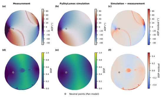
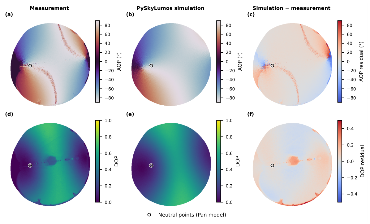
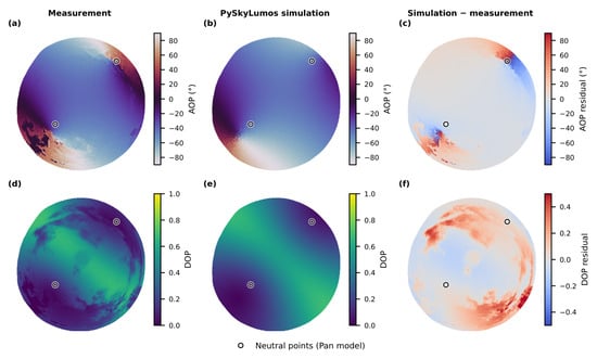
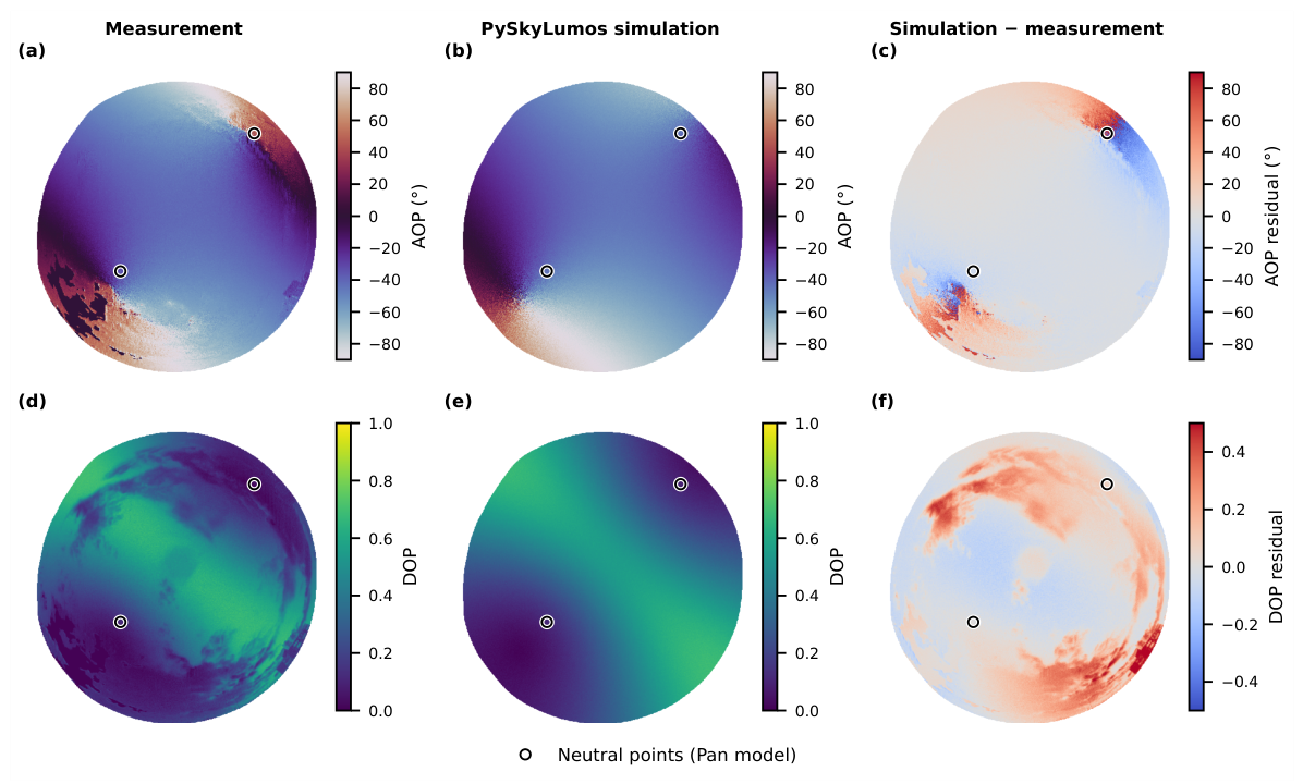
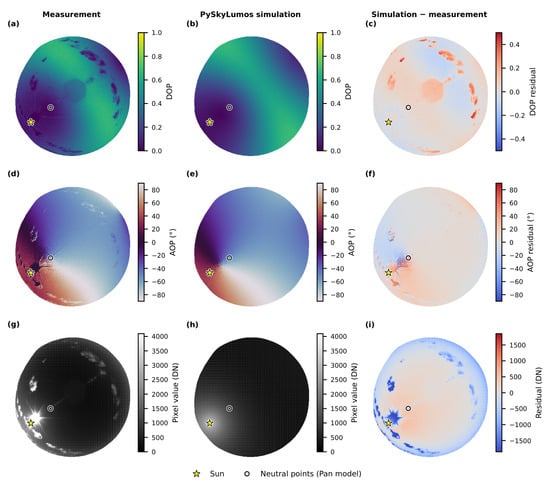
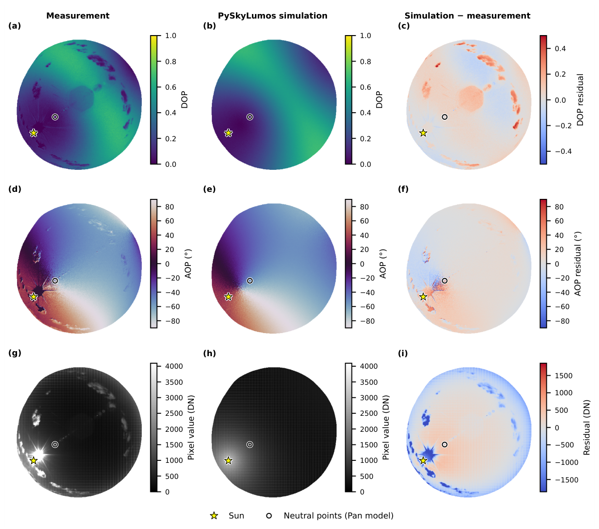
Figure 1, Figure 2 and Figure 3 share the same layout. The columns show the measurement, the Pan-model simulation, and the simulation minus the measurement, with AOP residuals wrapped to ±90°. Before comparison, the simulated DOP is scaled by an empirical maximum observable DOP of ${\mathrm{DOP}}_{max}=0.7$ (Equations (2) and (11)), which accounts for the depolarization of the real sky; the measured DOP is not scaled. The star marks the Sun and the circles the neutral points of the Pan model. Only the usable image area is shown: the camera rim, whose edge was measured in every direction from the Belmont intensity image (the same camera and lens were used at all sites), is excluded with a 20-pixel margin, which keeps the sky above an altitude of 12° to 22° depending on direction. The top of each image points East. The DoLP and azimuth values of the Liverpool and Bucharest pseudocolor exports were recovered from the documented full-scale ranges (0–100% and −90° to 90°).

Figure 1. Measurement, PySkyLumos simulation, and their difference for Liverpool on 11 November 2024 at 12:52 UTC: (a) measured AOP; (b) simulated AOP; (c) AOP difference; (d) measured DOP; (e) simulated DOP; (f) DOP difference. Differences are simulation minus measurement. The circle marks the neutral point predicted by the Pan model that lies within the usable image area. The Sun lies below the usable image area and is therefore not marked.

Figure 2. Measurement, PySkyLumos simulation, and their difference for Bucharest on 11 January 2025 at 13:47 UTC: (a) measured AOP; (b) simulated AOP; (c) AOP difference; (d) measured DOP; (e) simulated DOP; (f) DOP difference. Differences are simulation minus measurement. The circles mark the neutral points predicted by the Pan model that lie within the usable image area. The Sun lies below the usable image area and is therefore not marked.

Figure 3. Measurement, PySkyLumos simulation, and their difference for Belmont on 22 September 2025 at 15:05 UTC: (a) measured DOP; (b) simulated DOP; (c) DOP difference; (d) measured AOP; (e) simulated AOP; (f) AOP difference; (g) measured raw pixel values; (h) simulated raw pixel values; (i) raw pixel difference. Differences are simulation minus measurement. The star marks the Sun, and the circle marks the neutral point predicted by the Pan model that lies within the usable image area.

Figure 1 and Figure 2 compare the Liverpool and Bucharest recordings visually with the corresponding simulations; numerical errors are reported for the Belmont recording below, and approximate errors of all three sky models for every recording are given in Table 7. In both cases, the simulated and measured maps show the same overall AOP pattern and the band of maximum DOP at approximately 90° from the Sun. The residuals are largest near the edge of the usable image area, close to the neutral points, where the AOP changes rapidly, and in regions covered by clouds; at both sites the low Sun lies outside the usable image area.

Table 7. DOP and AOP errors of the three sky models over the usable image area.

Model	Error	Belmont (Sun at 24.6°)		Liverpool (17.9°)		Bucharest (9.2°)
		DOP	AOP (°)	DOP	AOP (°)	DOP	AOP (°)
Rayleigh	MAE	0.075	7.19	0.072	9.54	0.109	10.18
	RMSE	0.106	12.12	0.102	13.96	0.149	17.35
Berry	MAE	0.052	5.49	0.055	8.88	0.094	8.96
	RMSE	0.081	7.98	0.080	12.95	0.134	15.19
Pan	MAE	0.052	6.37	0.045	7.79	0.089	7.90
	RMSE	0.074	9.02	0.067	11.70	0.127	13.68

The simulation of the Belmont raw image used the Pan sky model, CIE standard sky type 8 (Equation (16)), a 15° azimuthal rotation, a 1° altitude clipping, the sensor parameters of Table 2 (Equations (18) and (19)), and a random seed of 9 for the sensor noise and the micro-polarizer orientation errors. The measured DOP and AOP were computed from the raw image with the same Stokes stage as the simulation (Equations (20)–(24)). The residuals concentrate near the Sun, where the measurement is saturated and affected by glare, and, as for Liverpool and Bucharest, near the edge of the usable image area and around the clouds visible in the raw image.

The mean absolute error (MAE) and the root mean square error (RMSE) were computed over the usable image area shown in Figure 3 to capture both the average deviation and the effect of outliers. The raw image simulation produced an MAE of 300 DN and an RMSE of 472 DN, and the degree of polarization an MAE of 0.052 and an RMSE of 0.074. The AOP describes the orientation of the electric-field oscillation rather than a direction, so an AOP and the same AOP plus 180° are physically identical: both produce the same pixel intensities and Stokes parameters (Equations (18)–(24)), which is why Equations (5), (10), and (24) all return values between −90° and 90°. AOP residuals are therefore wrapped to ±90°; for example, values of 89° and −89° differ by 2°, not 178°. The largest possible AOP difference is 90°, between perpendicular orientations, and the AOP errors were normalized by this maximum: a normalized value of 1 corresponds to the worst possible agreement, whereas a simulation uncorrelated with the sky would give a normalized MAE of 0.5. Near the neutral points, the light is so weakly polarized that the measured AOP is dominated by noise; the AOP errors were therefore computed only where the measured DOP is at least 0.05, which covers 94.6% of the usable image area. Over this region, the angle of polarization showed an MAE of 6.37° (normalized 0.071) and an RMSE of 9.02° (normalized 0.100).

To assess the simulation and sensor fidelity without the effects of the Sun and the clouds, which the clear-sky models do not represent, the errors were also computed over a clear-sky area. This area is the usable image area without (i) the pixels within 10° of the Sun, (ii) the super-pixels containing a saturated pixel (at least 4090 DN), extended by two super-pixels, and (iii) the clouds. Clouds were identified from the measurement alone, as super-pixels whose $S_0$ exceeds 1.25 times a median-filtered background over $61\times 61$ super-pixels, extended by three super-pixels. The clear-sky area covers 89% of the usable image area. Over it, the raw image simulation produced an MAE of 231 DN and an RMSE of 314 DN; the degree of polarization an MAE of 0.045 and an RMSE of 0.058; and, with the same DOP threshold (97.1% of the clear-sky area), the angle of polarization an MAE of 6.12° (normalized 0.068) and an RMSE of 8.49° (normalized 0.094).

The three sky models were also compared on all three recordings, with the same settings and metrics (Table 7). For Liverpool and Bucharest, the measured values are those recovered from the pseudocolor exports, so their errors are approximate: they include the quantization of the exports, of about 1.4° in AOP and 0.008 in DOP, and the clouds and glare that could not be masked without the raw images. At every site, both multiple-scattering models reduce the DOP error relative to the Rayleigh model. For the two low-Sun recordings, with the Sun at 17.9° and 9.2°, the Pan model gives the lowest DOP and AOP errors, consistent with its elevation-dependent neutral points and with the improvement over the Berry model reported by Pan et al. [7]. For the Belmont recording, with the Sun at 24.6°, the Berry model gives the lower AOP error, and the two models give similar DOP errors. With one recording per site, these results indicate a trend rather than a general ranking of the models.

4. Conclusions

We have presented PySkyLumos, an open-source Python framework for generating physically based skylight-polarization data with associated astronomical metadata. It implements the Rayleigh, Berry, and Pan models, covering single scattering, the splitting of the neutral points caused by multiple scattering, and the elevation-dependent motion of these points. With Astropy’s solar-ephemeris routines and automatic frame transformations, PySkyLumos produces polarization maps and singularity locations without the manual pre-processing required by previous tools.

Benchmarking against the open-source tool OpenSky [26] showed that PySkyLumos is about five times faster overall and about 150 (Apple) to 190 (Windows) times faster in the Stokes-parameter image formation. On the Apple platform, for example, one million full-resolution frames take about eight days of computation instead of about forty days with OpenSky, and the Stokes stage processes a 5 MP image in about 18 ms. PySkyLumos simulations were compared with sky images recorded with a polarization camera at three sites in the UK and Romania, with the Sun between 9° and 25° above the horizon. The simulated and measured polarization patterns agree closely: for the recording from Belmont, UK, for which the raw sensor data are available, the simulated angle of polarization (AOP) differs from the measured one by 6.12° on average over the cloud-free sky away from the Sun. Of the three sky models, the Pan model agreed best with the two recordings taken with the Sun lowest (9° and 18° above the horizon), and the Berry model gave the lowest AOP error for the recording with the highest Sun (25°). The largest differences arise from clouds and Sun glare (Figure 3), which the sky models do not represent; these are priorities for future updates, together with validation using further cameras and lenses.

In bio-inspired navigation, the heading is usually obtained from the solar meridian, which the AOP pattern identifies, and the position from the solar elevation combined with the time of day [20,21,22]. A database simulated with PySkyLumos can support both steps: a measured AOP and degree of polarization (DOP) map is compared with simulated maps for candidate headings, times, and locations, the best match gives the estimate, and the metadata provide the Sun and neutral-point positions of every candidate. The accuracy of such an estimate was not evaluated in this study. It depends on how many pixels are combined, so the per-pixel AOP error reported above is a reference for the input data rather than a heading error. Several mechanisms can cause misjudgement. Because the AOP is axial, the solar and anti-solar halves of the meridian produce the same AOP and must be distinguished by the intensity or DOP distribution. Near the neutral points and the horizon, the DOP is low and the measured AOP is dominated by noise. Clouds, Sun glare, and saturation distort the measured pattern locally, and a tilt of the sensor displaces the whole pattern unless it is measured and corrected [25]; PySkyLumos can simulate such tilts, so their effect on an estimator can be studied before deployment.

The applicability of the simulator follows from its models. None of the models describe Mie scattering by aerosols, haze, or water droplets explicitly: turbidity enters only through the CIE sky type and through ${\mathrm{DOP}}_{max}$, which lowers the DOP uniformly [26,38]. In the real sky, aerosol scattering also lowers the DOP non-uniformly and displaces the neutral points [3,37], and clouds alter the pattern locally, although the AOP pattern often continues beneath thin clouds [3]. PySkyLumos was found to be most accurate for clear skies with low turbidity, as in the clear-sky area of the Belmont recording, and its results should be interpreted with care under hazy, polluted, or cloudy conditions, where models that include aerosol scattering may be required.

Within these limits, PySkyLumos supports dataset generation, algorithm development and benchmarking, and instrument design, with applications in animal vision, bio-inspired computer vision, navigation, robotics, and atmospheric sensing.

References

- Collett, E. Field Guide to Polarization; SPIE Press: Bellingham, WA, USA, 2005; Volume 15. [Google Scholar]
- Goldstein, D.H. Polarized Light, 3rd ed.; CRC Press: Boca Raton, FL, USA, 2017. [Google Scholar] [CrossRef] [Scilit]
- Horváth, G. Polarization Vision and Environmental Polarized Light; Springer Nature: Berlin/Heidelberg, Germany, 2024. [Google Scholar] [CrossRef] [Scilit]
- Young, A.T. Rayleigh scattering. Phys. Today 1982, 35, 42–48. [Google Scholar] [CrossRef] [Scilit]
- Berry, M.; Dennis, M.; Lee, R. Polarization singularities in the clear sky. New J. Phys. 2004, 6, 162. [Google Scholar] [CrossRef] [Scilit]
- Berry, M. Nature’s optics and our understanding of light. Contemp. Phys. 2015, 56, 2–16. [Google Scholar] [CrossRef] [Scilit]
- Pan, P.; Wang, X.; Yang, T.; Pu, X.; Wang, W.; Bao, C.; Gao, J. High-similarity analytical model of skylight polarization pattern based on position variations of neutral points. Opt. Express 2023, 31, 15189–15203. [Google Scholar] [CrossRef] [Scilit] [PubMed]
- Waterman, T.H. Polarized light and animal navigation. Sci. Am. 1955, 193, 88–95. [Google Scholar] [CrossRef] [Scilit]
- Waldvogel, J.A. The Bird’s Eye View. Am. Sci. 1990, 78, 342–353. [Google Scholar]
- Wehner, R.d. Polarized-light navigation by insects. Sci. Am. 1976, 235, 106–115. [Google Scholar] [CrossRef] [Scilit] [PubMed]
- van den Berg, C.P.; Troscianko, J.; Endler, J.A.; Marshall, N.J.; Cheney, K.L. Quantitative Colour Pattern Analysis (QCPA): A comprehensive framework for the analysis of colour patterns in nature. Methods Ecol. Evol. 2020, 11, 316–332. [Google Scholar] [CrossRef] [Scilit]
- Cronin, T.W.; Shashar, N.; Caldwell, R.L.; Marshall, J.; Cheroske, A.G.; Chiou, T.H. Polarization Vision and Its Role in Biological Signaling. Integr. Comp. Biol. 2003, 43, 549–558. [Google Scholar] [CrossRef] [Scilit]
- Wang, Y.; Cai, J.; Louie, D.C.; Lui, H.; Lee, T.K.; Jane Wang, Z. Classifying Melanoma and Seborrheic Keratosis Automatically with Polarization Speckle Imaging. In Proceedings of the 2019 IEEE Global Conference on Signal and Information Processing (GlobalSIP), Ottawa, ON, Canada, 11–14 November 2019; pp. 1–4. [Google Scholar] [CrossRef] [Scilit]
- Rodríguez-Cortés, O.I.; Martínez-Ponce, G. Towards Skin Lesion Classification Using Machine Learning Algorithms and Stokes Imaging Polarimetry. In Proceedings of the 2024 Conference on Lasers and Electro-Optics Pacific Rim (CLEO-PR), Incheon, Republic of Korea, 4–9 August 2024; pp. 1–2. [Google Scholar] [CrossRef] [Scilit]
- Liu, Y.; Long, Y.; Cao, Y.; Liu, W.; Li, W. Three-dimensional model of cloud layers based on all-sky polarization imaging data. In Proceedings of the Ninth Symposium on Novel Photoelectronic Detection Technology and Applications, Hefei, China, 21–23 April 2023; Chu, J., Liu, W., Xu, H., Eds.; International Society for Optics and Photonics, SPIE: Bellingham, WA, USA, 2023; Volume 12617, p. 126171K. [Google Scholar] [CrossRef] [Scilit]
- Li, G.; Zhang, Y.; Fan, S.; Yu, F.; Wang, Y. Dynamic-Wave Interference Suppression Based on Angular Increment Assistance for Underwater Imaging Polarization Sensor. IEEE Trans. Instrum. Meas. 2025, 74, 5001713. [Google Scholar] [CrossRef] [Scilit]
- Su, F.; Wu, S.; Zhang, Z. A brief review of the photoelasticity based on a pixelated polarization camera: Principle, advantages/disadvantages and typical applications. J. Mech. 2024, 40, 698–710. [Google Scholar] [CrossRef] [Scilit]
- Choi, S.K.; Yang, Y.J.; Kim, K.N.; Choi, J.W.; Choi, Y.J.; Han, S.H. A Study of the Optical Properties of Cosmetics Measured by Polarized Light Goniophotometry. J. Opt. Soc. Korea 2012, 16, 36–41. [Google Scholar] [CrossRef] [Scilit]
- Xu, X.; Wu, J.; Wang, J.; Qu, Q.; Tan, Z.; Luo, M. Materials Identification of Polarized Pulse Laser Detection Based on Sparse Autoencoder and Softmax Classifier Framework. IEEE Trans. Instrum. Meas. 2022, 71, 1007609. [Google Scholar] [CrossRef] [Scilit]
- Karman, S.B.; Diah, S.Z.M.; Gebeshuber, I.C. Bio-inspired polarized skylight-based navigation sensors: A review. Sensors 2012, 12, 14232–14261. [Google Scholar] [CrossRef] [Scilit]
- Li, S.; Kong, F.; Xu, H.; Guo, X.; Li, H.; Ruan, Y.; Cao, S.; Guo, Y. Biomimetic Polarized Light Navigation Sensor: A Review. Sensors 2023, 23, 5848. [Google Scholar] [CrossRef] [Scilit] [PubMed]
- Kong, F.; Guo, Y.; Zhang, J.; Fan, X.; Guo, X. Review on bio-inspired polarized skylight navigation. Chin. J. Aeronaut. 2023, 36, 14–37. [Google Scholar] [CrossRef] [Scilit]
- Poughon, L.; Aubry, V.; Monnoyer, J.; Viollet, S.; Serres, J.R. An extended database of annotated skylight polarization images covering a period of two months. BMC Res. Notes 2024, 17, 306. [Google Scholar] [CrossRef] [Scilit] [PubMed]
- Liang, H.; Bai, H. Polarized skylight navigation simulation (PSNS) dataset. arXiv 2020, arXiv:2007.13081. [Google Scholar]
- Liang, H.; Bai, H.; Liu, N.; Shen, K. Limitation of Rayleigh sky model for bioinspired polarized skylight navigation in three-dimensional attitude determination. Bioinspir. Biomim. 2020, 15, 046007. [Google Scholar] [CrossRef] [Scilit] [PubMed]
- Moutenet, A.; Poughon, L.; Toulon, B.; Serres, J.R.; Viollet, S. OpenSky: A modular and open-source simulator of sky polarization measurements. IEEE Trans. Instrum. Meas. 2024, 73, 5014716. [Google Scholar] [CrossRef] [Scilit]
- Ciochirca, T.A.; Chadwick, D.J.; Sandall, I.; Ralph, J.F. PySkyLumos (GitHub). 2025. Available online: https://github.com/taciochi/pyskylumos (accessed on 7 October 2026).
- Ciochirca, T.A.; Chadwick, D.J.; Sandall, I.; Ralph, J.F. PySkyLumos (Python Package Index), Version 0.0.5. 2025. Available online: https://pypi.org/project/pyskylumos/0.0.5/ (accessed on 7 October 2026).
- Hosek, L.; Wilkie, A. An analytic model for full spectral sky-dome radiance. ACM Trans. Graph. (TOG) 2012, 31, 1–9. [Google Scholar] [CrossRef] [Scilit]
- Hošek, L.; Wilkie, A. Adding a solar-radiance function to the hošek-wilkie skylight model. IEEE Comput. Graph. Appl. 2013, 33, 44–52. [Google Scholar] [CrossRef] [Scilit] [PubMed]
- LUCID Vision Labs. Phoenix 5.0 MP Polarization Camera (Sony IMX250MZR/MYR). 2024. Available online: https://thinklucid.com/product/phoenix-5-0-mp-polarized-model/ (accessed on 23 May 2024).
- Sony Semiconductor Solutions Corporation. IMX250/264/253MZR/MYR: Polarization Image Sensor with Four-Directional on-Chip Polarizer and Global Shutter Function. Product Flyer, Sony Semiconductor Solutions Corporation. 2021. Available online: https://www.sony-semicon.com/files/62/flyer_industry/IMX250_264_253MZR_MYR_Flyer_en.pdf (accessed on 23 May 2024).
- Liang, H.; Bai, H.; Liu, N.; Shen, K. Hypothetical Polarization Camera. 2020. Available online: https://github.com/HuajuLiang/HypotheticalPolarizationCamera (accessed on 2 April 2025).
- Liang, H.; Bai, H. Original Light Intensity. 2020. Available online: https://github.com/HuajuLiang/OriginalLightItensity/tree/master (accessed on 2 April 2025).
- Wilkie, A.; Ulbricht, C.; Tobler, R.F.; Zotti, G.; Purgathofer, W. An analytical model for skylight polarisation. In Proceedings of the Rendering Techniques, Norrköping, Sweden, 21–23 June 2004; pp. 387–398. [Google Scholar]
- Li, D.; Li, C.; Lou, S.; Tsang, E.; Lam, J. Analysis of vertical sky components under various CIE standard general skies. Indoor Built Environ. 2016, 25, 703–711. [Google Scholar] [CrossRef] [Scilit]
- Wang, X.; Gao, J.; Fan, Z.; Roberts, N.W. An analytical model for the celestial distribution of polarized light, accounting for polarization singularities, wavelength and atmospheric turbidity. J. Opt. 2016, 18, 065601. [Google Scholar] [CrossRef] [Scilit]
- Darula, S.; Kittler, R. CIE general sky standard defining luminance distributions. Proc. eSim. 2002, 11, 13. [Google Scholar]
- Hou, W.; Ding, M.; Qin, N.; Lai, X. Digital deformation model for fisheye image rectification. Opt. Express 2012, 20, 22252–22261. [Google Scholar] [CrossRef] [Scilit] [PubMed]
- Moutenet, A.; Poughon, L.; Toulon, B.; Serres, J.R.; Viollet, S. OpenSky GitHub. 2024. Available online: https://github.com/MoutenetA/OpenSky (accessed on 2 April 2025).
- Clarke, D. Stellar Polarimetry; John Wiley & Sons: Hoboken, NJ, USA, 2009. [Google Scholar]
- Brewster, D. LXVIII. On the polarization of the atmosphere. Lond. Edinb. Dublin Philos. Mag. J. Sci. 1847, 31, 444–454. [Google Scholar] [CrossRef] [Scilit]
- Harris, C.R.; Millman, K.J.; van der Walt, S.J.; Gommers, R.; Virtanen, P.; Cournapeau, D.; Wieser, E.; Taylor, J.; Berg, S.; Smith, N.J.; et al. Array programming with NumPy. Nature 2020, 585, 357–362. [Google Scholar] [CrossRef] [Scilit]
- Gorelick, M.; Ozsvald, I. High Performance Python: Practical Performant Programming for Humans; O’Reilly Media: Santa Rosa, CA, USA, 2020. [Google Scholar]
- Python Core Team. Python: A Dynamic, Open Source Programming Language, Version 3.12.2; Python Software Foundation: Beaverton, OR, USA, 2025. [Google Scholar]
- Price-Whelan, A.M.; Lim, P.L.; Earl, N.; Starkman, N.; Bradley, L.; Shupe, D.L.; Patil, A.A.; Corrales, L.; Brasseur, C.E.; Nöthe, M.; et al. The Astropy Project: Sustaining and Growing a Community-oriented Open-source Project and the Latest Major Release (v5.0) of the Core Package. Astrophys. J. 2022, 935, 167. [Google Scholar] [CrossRef] [Scilit]
- Slater, J.A.; Malys, S. WGS 84—Past, Present and Future. In Proceedings of the Advances in Positioning and Reference Frames, Rio de Janeiro, Brazil, 3–9 September 1997; Brunner, F.K., Ed.; Springer: Berlin/Heidelberg, Germany, 1998; pp. 1–7. [Google Scholar]
- Moisson, X.; Bretagnon, P. Analytical planetary solution VSOP2000. Celest. Mech. Dyn. Astron. 2001, 80, 205–213. [Google Scholar] [CrossRef] [Scilit]
- Moiseev, Y.A.; Emelyanov, N.V. Ephemeris Theories JPL DE, INPOP, and EPM. Astron. Rep. 2024, 68, 1098–1118. [Google Scholar] [CrossRef] [Scilit]
- Fujinon, F. Fujinon FE185C057HA-1 Technical Datasheet. 2023. Available online: https://downloads.machinevisiondirect.com/wp-content/uploads/Fujinon/FE185C057HA-1/FE185C057HA-1_Datasheet.pdf (accessed on 16 September 2025).
Disclaimer/Publisher’s Note: The statements, opinions and data contained in all publications are solely those of the individual author(s) and contributor(s) and not of MDPI and/or the editor(s). MDPI and/or the editor(s) disclaim responsibility for any injury to people or property resulting from any ideas, methods, instructions or products referred to in the content. |
© 2026 by the authors. Licensee MDPI, Basel, Switzerland. This article is an open access article distributed under the terms and conditions of the Creative Commons Attribution (CC BY) license.