Improved Pointwise Ensemble Surrogate Modelling for Assembly Deviation Analysis of Thin-Walled Parts

Abstract

For assembly deviation analysis of thin-walled parts, single surrogate models are suitable for cases with simple assembly processes and few design variables. For complex parts with high flexibility, nonlinear behavior, and variable spring-back effects, ensemble surrogate models are more suitable. To address the deficiencies of the existing Pointwise Ensemble with Adaptive Function and Heuristic Formulation (PEAH) in terms of the continuity of the weight function and local adaptability, this paper proposes an improved kernel-weighted method, denoted as KW-PEAH. Specifically, it introduces a Gaussian kernel function to replace linear distance weighting for smooth distance decay, and employs a K-nearest neighbor (KNN) strategy to dynamically adjust the kernel bandwidth based on local sample density. KW-PEAH was compared with four ensemble methods and the original PEAH, using eight benchmark functions and a simulation-based thin-walled assembly case under noise. Compared with the PEAH method, the NRMSE values on the BH and ER functions are reduced by approximately 6.2% and 2.9%, respectively. In the simulation-based thin-walled assembly case, KW-PEAH achieves lower RMSE and MAE and higher mean R² at all three noise levels. Under the 10% noise level, the mean RMSE and MAE are reduced by approximately 6.7% and 5.6%. Overall, the results indicate that KW-PEAH is suited for thin-walled part deviation analysis in low- to medium-dimensional, noisy scenarios.

1. Introduction

Thin-walled parts are widely used in aerospace, automotive, precision machinery, and other fields. However, their large dimensions and low structural rigidity make thin-walled parts particularly susceptible to deformation. During assembly, manufacturing deviations and positioning errors can induce elastic or even plastic deformation, thereby compromising assembly accuracy and in-service performance [1]. Therefore, to ensure the reliability and stability of products in actual use, extensive assembly deviation simulations must be carried out at the design stage to support the analysis and optimization of assembly accuracy for thin-walled parts. Conducting accurate and efficient analysis of assembly deviations for thin-walled parts has become a research question of significant academic value [2,3].

Current mainstream assembly deviation analysis methods include finite element simulation [4,5,6], Monte Carlo simulation [7,8,9], and the influence coefficient method [10,11,12]. Although finite element analysis offers high accuracy, it is computationally expensive; Monte Carlo simulation is simple but time-consuming; the influence coefficient method is practical yet limited for nonlinear problems. In recent years, physics-informed and data-driven techniques, such as physics-informed neural networks, operator-learning models and generative models, have provided new opportunities for thin-walled structural analysis [13,14,15]. However, their applicability and computational requirements vary with the problem formulation and data availability. For engineering problems involving limited simulation samples and repeated prediction requirements, surrogate modeling [16] remains an attractive alternative because it provides computationally efficient approximations of high-fidelity simulation responses, thereby reducing the computational burden of repeated analyses.

However, a single surrogate model may not simultaneously achieve global accuracy, local nonlinearity capture, and noise robustness—particularly in thin-walled assembly deviation analysis. Consequently, ensemble surrogate models [17] that combine multiple base models have become an effective approach to improving prediction performance.

Common ensemble strategies can be broadly classified into three categories according to their weight assignment mechanisms. The first category is global fixed-weight ensemble, which adopts either a uniform weight or weights pre-computed based on overall error for all prediction points—for example, uniform averaging [18] and inverseRMSE-weighted ensemble [19]. Hu et al. [20] proposed a conservative multi-fidelity weighted-average ensemble method for robust optimization under uncertainty, while Lu et al. [21] developed an adaptive-weight ensemble based on distance and mixed-error information. The second category is global adaptive-weight ensemble, where weights are dynamically computed using optimization algorithms or probabilistic frameworks, such as Bayesian averaging ensemble [22]. Li et al. [23] developed a Bayesian averaging surrogate framework to address structural uncertainty and improve response prediction efficiency. The third category is local point-wise ensemble [24], which independently computes weights or performs local optimization for each prediction point, dynamically adjusting the contribution of each base model. Liu et al. [25] proposed the OWPE method, which optimizes local weights of radial basis-function models using observation-point weights and a decay coefficient. Hao et al. [26] proposed the PEAH method, which builds a point-wise ensemble surrogate model that fuses local accuracy and prediction uncertainty information, introducing an adaptive function and a heuristic weighting formula to calculate and adjust the weights of each base model, thus achieving higher prediction accuracy and stronger robustness. Moreover, their study validated the performance of PEAH through multiple test functions and two engineering tests, comprehensively evaluating its performance under various conditions and engineering scenarios. Their results indicate that PEAH can provide competitive or improved prediction performance compared with several existing global and pointwise ensemble strategies, particularly for problems involving strong nonlinearity or complex local features.

Despite these advantages, the local weighting mechanism of PEAH remains amenable to further improvement. Its local characteristic function is constructed using a distance-based weighting scheme. In practical implementations, particularly when a finite neighborhood is used or when local error estimates vary rapidly, this distance-based scheme may lead to abrupt variations in the estimated local accuracy and the resulting ensemble weights. Such fluctuations may reduce the smoothness and stability of the ensemble predictions, especially in sparse or noisy regions. To mitigate these effects, Gaussian kernel weighting [27,28] is introduced to provide a smoother distance-decay mechanism. For example, Wang et al. [29] applied Gaussian kernel weighting to response-surface reconstruction, whereas Zhu et al. [30] used it to improve deformation prediction robustness for noisy thin-walled structures. These studies suggest that Gaussian kernel weighting can improve prediction continuity and robustness in relevant modeling problems. However, a fixed kernel width cannot adapt to different scenarios and lacks dynamic adjustment capability. To address this limitation, a K-nearest neighbor (KNN)-based strategy [31,32] can be used to adapt the kernel bandwidth to the local sample distribution. This strategy determines a dedicated bandwidth for each prediction point based on the median distance between the point and its K-nearest training samples, thereby adapting the kernel influence range to the local sample density. Deoraoji et al. [33] developed an adaptive bandwidth method for non-uniform kernel regression, and Xia et al. [34] demonstrated the effectiveness of KNN-based local-density characterization. Building upon these studies, this paper proposes an improved pointwise ensemble strategy. The method replaces the linear distance weighting in PEAH with Gaussian kernel weighting and employs a KNN-based adaptive bandwidth strategy to account for local variations in sample density.

In summary, to address the limitations of the local weighting mechanism of PEAH, this paper proposes an improved pointwise ensemble method, Kernel-Weighted PEAH (KW-PEAH). The remainder of this paper is organized as follows: Section 2 presents the PEAH model and the proposed KW-PEAH method. Section 3 describes the experimental design based on benchmark functions and a simulation case. Section 4 presents a comparative analysis of the results, systematically evaluating the comprehensive performance of the proposed method on both test functions and simulation cases. Section 5 summarizes the main findings, limitations, and directions for future research.

2. KW-PEAH Method

2.1. Overall Framework

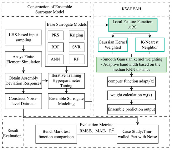
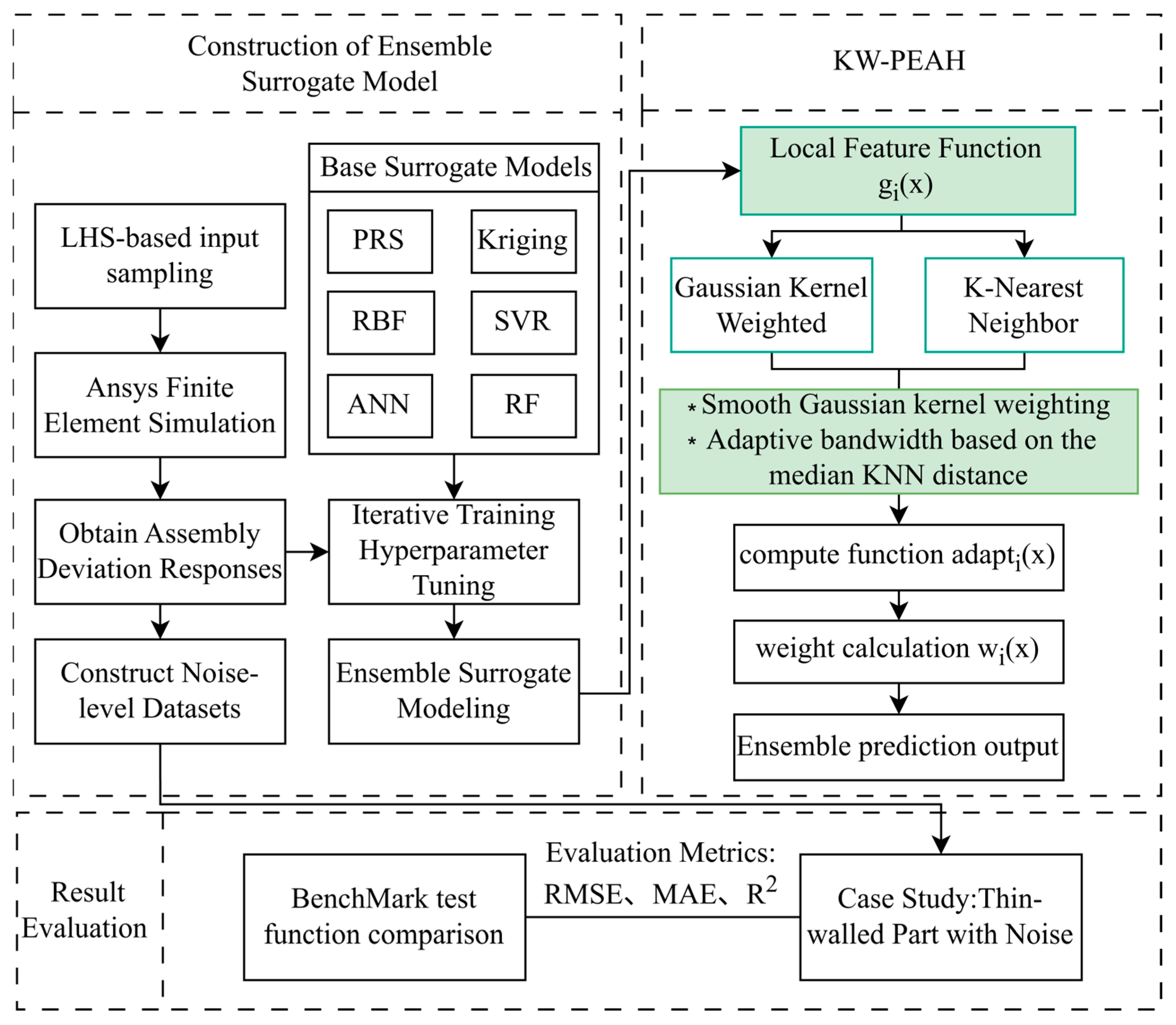
This study is based on the PEAH ensemble method. First, for the determined design variables, an initial sample set is established through sampling via a design of experiments method, and the finite element software is used to compute the sample responses, providing the dataset for the surrogate model. In the PEAH method, when constructing the ensemble model, a local characteristic function based on linear distance weighting is computed, which is then combined with an adaptive function for calculation, and finally the ensemble prediction results are generated. This paper replaces the linear weighting with Gaussian kernel-weighted regression and introduces the K-nearest neighbor algorithm to achieve adaptive adjustment of the kernel bandwidth. The effectiveness of the proposed method is subsequently evaluated using benchmark functions and a thin-walled assembly case under noisy conditions. The methodological framework is shown in Figure 1.

Figure 1. Framework of the KW-PEAH method. *: Improvements of KW-PEAH compared to PEAH.

2.2. PEAH Model

The PEAH method [26] combines an adaptive function and heuristic weight calculation. By incorporating local accuracy and uncertainty information at the prediction point, it is able to adapt to the characteristics of local uncertainties. The weight calculation formula is as follows:

$$w_i(x)={\displaystyle \frac{{\left[E_i(x)+\alpha \overline{E}(x)\right]}^{\beta }}{{\displaystyle {\sum }_{k=1}^M{\left[E_k(x)+\alpha \overline{E}(x)\right]}^{\beta }}}}$$

(1)

where w_i(x) is the adaptive weight of the ith surrogate model at the prediction point, E_i(x) is the local adaptive error of the ith base model at the prediction point, α and β represent the averaging coefficient and the penalty coefficient, respectively, which depend on $\sqrt{\mathit{GMSE}}$ and are then solved using the fmincon function in conjunction with the SQP optimizer [35]. Here, $\overline{E}(x)$ is the average of the local errors of all models.

E_i(x) = E_i ⋅ adapt_i(x)

(2)

The global error E_i is defined as the global root mean square error $\sqrt{\mathit{GMSE}}$ on the training set, i.e.:

$$E_i=\sqrt{\mathit{GMSE}}=\sqrt{{\displaystyle \frac{1}{N}}{\displaystyle {\sum }_{i=1}^M{\left(y-{\widehat{y}}_i\right)}^2}}$$

(3)

where N is the total number of sample points in the training set, and M is the number of base surrogate models. Here, y denotes the true response value of the training sample, and ${\widehat{y}}_i$ is the predicted value of the ith base surrogate model for that training sample. In Equation (2), adapt_i(x) represents the adaptive function of the ith surrogate model at the prediction point x, which is computed as follows:

$${\mathit{adapt}}_i(x)=g_i{(x)}^{\left[1+e^{-1/u(x)}\right]}$$

(4)

where g_i(x) is the local characteristic function of the ith surrogate model at the prediction point x, calculated as:

g_i(x) = d(x)^T ⋅ ac_i

(5)

where $d(x)={\left[d(x,x_1),d(x,x_2),\cdots d(x,x_N)\right]}^T$ denotes the distance vector, d(x,x_N) represents the Euclidean distance between the prediction point and the Nth training point, and ac_i denotes the normalized cross-validation error vector of the ith model over all training points:

$$a{c}_i={\left[{\tilde{e}}_i(x_1),{\tilde{e}}_i(x_2),\dots {\tilde{e}}_i(x_N)\right]}^T$$

(6)

where ${\tilde{e}}_i(x_N)$ represents the pointwise cross-validation error of the ith surrogate model at the training point N, computed as:

$${\tilde{e}}_i(x_N)={\displaystyle \frac{\left|e_i(x_N)\right|}{{\displaystyle {\sum }_{i=1}^M\left|e_i(x_N)\right|}}}$$

(7)

In Equation (4), u_i(x) denotes the uncertainty of the local accuracy of all surrogate models at the prediction point x, calculated as:

$$u(x)=\sqrt{{\displaystyle \frac{1}{M-1}}{\displaystyle {\sum }_{i=1}^M{\left[g_i(x)-\overline{g}(x)\right]}^2}}$$

(8)

where ${\overline{g}}_i(x)$ represents the average of the local characteristic functions g_i(x) of the M base surrogate models at the prediction point x, calculated as:

$$\overline{g}(x)={\displaystyle \frac{{\displaystyle {\sum }_{i=1}^M{g}_i(x)}}{M}}$$

(9)

In Equation (9), a larger value of u(x) indicates higher uncertainty in the local accuracy of the region near the prediction point x. By combining the local characteristic function g_i(x) and the adaptive function adapt_i(x), the weights of the surrogate models are computed via Equation (1), thereby constructing the PEAH ensemble surrogate model.

2.3. Limitations of PEAH

The PEAH method combines global error with variations at the prediction point x through a local adaptive function, thereby endowing the weights with pointwise characteristics. Its local characteristic function is essentially based on linear distance weighting, i.e., the farther the distance, the smaller the contribution. Two main shortcomings can be summarized as follows:

(1)

Limited smoothness of the distance-based weighting mechanism: In the local characteristic function of the PEAH method, the linear combination of distances, i.e., d(x)^T ⋅ ac_i, is used to construct the local characteristic function. However, it is not smoothly differentiable at the sample location because the Euclidean distance d_i(x) = ‖x − x_i‖ is not differentiable at x = x_i. Moreover, when a finite neighborhood is imposed in practical implementations, the commonly used linear weight has a discontinuous first derivative at the neighborhood boundary. This lack of smoothness may cause abrupt changes in the local error estimate when the prediction point moves across a sample point or a neighborhood boundary. Such changes can subsequently be amplified by the adaptive and heuristic weighting procedure, resulting in local oscillations in the ensemble prediction.

(2)

Lack of adaptive adjustment capability for neighborhood influence range: The PEAH method cannot adaptively adjust the influence radius according to local sample density or noise level. In regions with high noise or uneven sample distribution, local oscillations are prone to occur, which reduces the continuity and stability of predictions.

Therefore, based on the above analysis, a smoother and adaptively adjustable local weighting mechanism can be introduced to enhance the stability and continuity of the PEAH model in engineering problems.

2.4. Improvement Ideas and Methodology

To address the above issues, drawing on the idea of kernel regression, this paper proposes an adaptive kernel-weighted pointwise ensemble method (KW-PEAH), which replaces the original linear distance weighting with Gaussian kernel weighting, so that the influence of each training sample within the neighborhood on the current prediction point decays smoothly and continuously with distance. An adaptive kernel bandwidth adjustment strategy based on KNN, i.e., the median distance of local nearest neighbors, is introduced to enable the influence range of the kernel function to be dynamically adjusted according to the local sample density, thereby potentially enhancing the stability and robustness of the error field smoothing, and contributing to improved continuity and noise resistance of the predictions

Specifically, Gaussian kernel weighting assigns larger weights to samples close to the prediction point, while the contributions of more distant samples decrease gradually according to an exponential decay function. Compared with the linear distance weighting used in the original PEAH method, this formulation provides a smoother weighting transition and helps reduce local oscillations caused by abrupt changes in sample contributions.

The improved kernel-weighted local characteristic function is given as follows:

$$g_i^{\mathit{KW}}(x)={\displaystyle \sum _{k=1}^N{K}_h\left(‖x-x_k‖\right)\cdot a{c}_{i,k}}$$

(10)

where ‖x − x_k‖ denotes the Euclidean distance between the prediction point and the sample point x_k, ac_i,k is the normalized pointwise cross-validation error of the ith base model at the kth training point, and K_h(r) is the Gaussian kernel function:

$$K_h(r)=\exp \left(-{\displaystyle \frac{r^2}{2h{(x)}^2}}\right)$$

(11)

where r is ‖x − x_k‖, representing the Euclidean distance between the prediction point and the sample point, and h(x) denotes the Gaussian kernel width. To adapt to the local sample distribution, this paper adopts an adaptive strategy that adjusts the weight based on the median distance of local nearest neighbors, defined as:

h(x) = c ⋅ median_k(‖x − x_k‖), k ∈ nearest(x,k)

(12)

where nearest(x,k) denotes the set of the k training sample points closest to the current prediction point x, and c is the adjustment coefficient. The values of the number of nearest neighbors k and the adjustment coefficient c directly affect the kernel bandwidth. To determine a reasonable parameter configuration, a sensitivity analysis will be conducted and discussed in Section 3.4.

The subsequent solution process is consistent with that of the original PEAH method. To systematically verify the effectiveness of the above improvements, the experimental design and comparative results are presented in Section 3 and Section 4, respectively.

2.4.1. Rationale for Gaussian Kernel Weighting

To clarify the effect of the proposed modification, let d_i(x) = ‖x − x_i‖ denote the Euclidean distance between a prediction point x and the ith training sample x_i. The original PEAH local characteristic function employs a linear weight, calculated as:

$$w_i^L\left(x\right)=\left[1-{\displaystyle \frac{d_i\left(x\right)}{r}}\right]$$

(13)

whose gradient is discontinuous at both the sample points (x = x_i) and the neighborhood boundary (d_i(x) = r). These discontinuities can induce abrupt changes in the local error estimate and subsequent ensemble weights, leading to local oscillations.

In contrast, the Gaussian kernel weight

$$w_i^G\left(x\right)=\exp \left(-{\displaystyle \frac{d_i^2\left(x\right)}{2h^2\left(x\right)}}\right)$$

(14)

is infinitely differentiable for any fixed h > 0. Its gradient vanishes at x = x_i and remains bounded, thus avoiding sharp variations:

$$‖\nabla w_i^G\left(x\right)‖\le {\displaystyle \frac{1}{h\sqrt{e}}}$$

(15)

Consequently, the kernel-weighted local characteristic function varies smoothly with the prediction location, provided that the bandwidth is fixed. This smoothness is expected to reduce abrupt variations in the local error estimate and to improve the stability of the resulting pointwise ensemble weights.

Other kernel functions, such as the Epanechnikov and triangular kernels, may also be used to construct the local characteristic function. However, both kernels have compact support, such that samples outside a prescribed distance are assigned zero weight. Under non-uniform sampling, the contribution of samples near the support boundary may therefore change more rapidly as the prediction point moves. In addition, the triangular kernel is piecewise linear and is not differentiable at its center, whereas the Epanechnikov kernel has a finite-support boundary. In contrast, the Gaussian kernel provides an infinitely differentiable weighting function with gradual distance decay and nonzero, albeit diminishing, contributions from distant samples. These properties are consistent with the objective of mitigating local weight fluctuations in sparse or noisy regions. Therefore, the Gaussian kernel is selected in this study based on its smoothness, gradual distance decay, and compatibility with the adaptive bandwidth strategy.

2.4.2. Rationale for Median-Based Adaptive Bandwidth Selection

The median distance is selected instead of the mean distance because it provides a robust estimate of the local spatial scale. Under a locally constant sampling density f(x) in a p-dimensional input space, the jth nearest neighbor distance approximately satisfies [36]:

$$d_{\left(j\right)}\left(x\right)\approx {\left({\displaystyle \frac{j}{n{V}_{p}f\left(x\right)}}\right)}^{1/p}$$

(16)

where n is the training-sample size and V_p is the volume of a unit p-dimensional ball. Consequently, the median distance to the K-nearest neighbors is approximately inversely related to the local sample density. In dense regions, the median distance is small and a narrower bandwidth is used to preserve local response features. In sparse regions, the median distance increases and the kernel bandwidth expands automatically, allowing more distant samples to contribute to the local error estimate and reducing estimation variance.

Compared with the mean, the median is less sensitive to extreme distances and isolated outliers, preventing excessively large bandwidths caused by the sample sparsity or noise. The minimum distance may produce an overly narrow bandwidth due to local clustering, whereas the maximum distance may lead to excessive smoothing. Therefore, the median provides a robust and computationally simple estimate of the local sample scale, while retaining the density-adaptive property of KNN bandwidth selection. Although it is not universally optimal, it is well suited to noisy and non-uniform sample distributions in thin-walled assembly deviation problems.

2.5. Computational Complexity

Compared with the original PEAH, the additional computational cost of KW-PEAH mainly stems from two sources:

(1)

The KNN search for determining the adaptive bandwidth h(x) at each prediction point;

(2)

The evaluation of the Gaussian kernel function.

For a training set of size N and M prediction points, KNN search requires computing distances between every prediction point and every training sample, resulting in a computational complexity of O(MN). In practice, with a modest k and the use of efficient data structures, the cost can be reduced appropriately. The subsequent Gaussian kernel evaluation is O(Mk), which is negligible. Actually, in typical thin-walled assembly deviation problems, the dominant computational cost arises from high-fidelity finite-element analyses or the training of the base surrogate models, rather than from the ensemble prediction step. The computational cost comparison between PEAH and KW-PEAH is presented in Section 4.2.2.

3. Experimental Comparison Design

To comprehensively verify the prediction performance and engineering applicability of the proposed KW-PEAH method, six ensemble strategies are compared in this study: uniform averaging (UA) [18], inverse-RMSE-weighted ensemble (IRMSE) [19], Bayesian averaging (BA) [22], optimal weighted pointwise ensemble (OWPE) [25], the original PEAH method, and the proposed KW-PEAH method. The same six classic base surrogate models, namely PRS, Kriging, RBF, SVR, ANN, and RF, are used in all ensemble strategies to ensure a fair comparison.

The experimental investigation is conducted from two perspectives: typical test functions and a simulation case. On one hand, eight classical test functions [37] widely used in the literature are selected as benchmarks to systematically evaluate the performance of the proposed method under various complex response surfaces. On the other hand, a practical thin-walled assembly-deviation problem is considered to further evaluate the engineering applicability of the proposed method. In this paper, three classical performance metrics, namely Root Mean Square Error (RMSE), Mean Absolute Error (MAE), and Coefficient of Determination (R²) [38], are adopted to quantify and compare the overall performance of different ensemble methods.

To ensure a fair comparison, all ensemble methods used the same training–test partitions, data-preprocessing procedures, cross-validation folds, and evaluation metrics in each trial.

3.1. Classical Test Functions

(1)

Branin–Hoo (BH): A two-dimensional function for testing the global exploration capability of optimization algorithms.

$$\begin{array}{c}f(x)={\left[x_2-5.1{(x_1/2\pi )}^2+(5/\pi )x_1-6\right]}^2+10\left[1-(1/8\pi )\right]\cos x_1+10\\ x_1\in \left[-5,10\right],x_2\in \left[0,15\right]\end{array}$$

(17)

(2)

Camelback (CB): A two-dimensional function for examining the local search and balance capability of the model.

$$\begin{array}{c}f(x)=4x_1^2-2.1x_1^4+x_1^6/3+x_1{x}_2-4x_2^2+4x_2^4\\ x_1\in \left[-3,3\right],x_2\in \left[-2,2\right]\end{array}$$

(18)

(3)

Goldstein–Price (GF): A two-dimensional function for evaluating the nonlinear fitting accuracy of surrogate models.

$$\begin{array}{c}f(x)=\left[1+{\left(x_1+x_2+1\right)}^2\left(19-14x_1+3x_1^2-14x_2+6x_1{x}_2+3x_2^2\right)\right]\cdot \\ \left[30+{(2x_1-3x_2)}^2(18-32x_1+12x_1^2+48x_2-36x_1{x}_2+27x_2^2)\right],x\in {\left[-2,2\right]}^2\end{array}$$

(19)

(4)

Hartman3 (HN3): A three-dimensional function that can effectively simulate complex multimodal response surfaces in engineering.

$$\begin{array}{c}f(x)=-{\displaystyle \sum _{i=1}^4{c}_i\exp \left[-{{\displaystyle \sum _{j=1}^n{a}_{\mathit{ij}}(x_j-p_{\mathit{ij}})}}^2\right]},x\in {\left[0,1\right]}^n\\ a_{\mathit{ij}}=\left[\begin{array}{ccc}3& 10& 30\\ 0.1& 10& 35\\ 3& 10& 30\\ 0.1& 10& 35\end{array}\right],p_{\mathit{ij}}=\left[\begin{array}{ccc}0.3689& 0.1170& 0.2673\\ 0.4699& 0.4387& 0.7470\\ 0.1091& 0.8732& 0.5547\\ 0.03815& 0.5743& 0.8828\end{array}\right],c_i=\left[\begin{array}{c}1\\ 1.2\\ 3\\ 3.2\end{array}\right]\end{array}$$

(20)

(5)

Shekel (SK): A four-dimensional function for testing the local interpolation accuracy of surrogate models.

$$\begin{array}{c}f(x)=-{\displaystyle \sum _{i=1}^5{\left({\displaystyle \sum _{j=1}^n{(x_j-a_{\mathit{ij}})}^2}+c_i\right)}^{-1}},x\in {\left[0,10\right]}^n\\ \left[a_{\mathit{ij}}\right]=\left[\begin{array}{cccc}4& 4& 4& 4\\ 1& 1& 1& 1\\ 8& 8& 8& 8\\ 6& 6& 6& 6\\ 3& 7& 3& 7\end{array}\right],c_i=\left[\begin{array}{ccccc}0.1& 0.2& 0.2& 0.4& 0.4\end{array}\right]\end{array}$$

(21)

(6)

Hartman6 (HN6): A six-dimensional extension of the Hartman function, used to test algorithm performance in high-dimensional multimodal scenarios.

$$\begin{array}{c}f(x)=-{\displaystyle \sum _{i=1}^4{c}_i\exp \left[-{{\displaystyle \sum _{j=1}^n{a}_{\mathit{ij}}(x_j-p_{\mathit{ij}})}}^2\right],i=1,2,\dots },n\\ \left[a_{\mathit{ij}}\right]=\left[\begin{array}{cccccc}10& 3& 17& 3.5& 1.7& 8\\ 0.05& 10& 17& 0.1& 8& 14\\ 3& 3.5& 1.7& 10& 17& 8\\ 17& 8& 0.05& 10& 0.1& 14\end{array}\right],\left[p_{\mathit{ij}}\right]=\left[\begin{array}{cccccc}1312& 1696& 5569& 124& 8283& 5886\\ 2329& 4135& 8307& 3736& 1004& 9991\\ 2348& 1451& 3522& 2883& 3047& 6650\\ 4047& 8828& 8732& 5743& 1091& 381.5\end{array}\right]\times {10}^{-4}\\ c_i=\left[\begin{array}{cccc}1& 1.2& 3& 3.2\end{array}\right],x\in {\left[0,1\right]}^n\end{array}$$

(22)

(7)

Extended Rosenbrock (ER): A nine-dimensional extension of the Rosenbrock function, used to test the global fitting and generalization ability of the model.

$$f(x){\displaystyle \sum _{i=1}^{n-1}\left[{(1-x_i)}^2+100{\left(x_{i+1}-x_i^2\right)}^2\right]},x\in {\left[-5,10\right]}^n$$

(23)

(8)

Dixon–Price (DP): A twelve-dimensional generalized quadratic function with chain-dependent relationships among variables, mainly used to examine the scalability of surrogate model methods in high-dimensional problems.

$$f(x)={(x_1-1)}^2+{\displaystyle \sum _{i=2}^{n}i{(2x_i^2-x_{i-1})}^2,x\in {\left[-10,10\right]}^n}$$

(24)

The Latin Hypercube Sampling (LHS) method is adopted to generate the datasets. Depending on the number of input variables, the training set for each test problem consists of 12 to 182 points. To reduce the influence of random sampling, 1000 different training sets are used for all test problems. Table 1 summarizes the training and testing data used for the test problems.

Table 1. Training and testing data for the test problems.

Fun.	No. of Design Variables	Training Points	Test Points	No. of Training Sets
BH	2	12	441	1000
CB	2	12	441	1000
GF	2	12	441	1000
HN3	3	36	512	1000
SK	4	36	512	1000
HN6	6	56	512	1000
ER	9	110	1000	1000
DP	12	182	1000	1000

The eight benchmark functions cover different dimensions and response-surface characteristics, enabling the proposed method to be evaluated under diverse modeling conditions. The corresponding results are presented and analyzed in Section 4.1.

3.2. Simulation Case of Thin-Walled Assembly

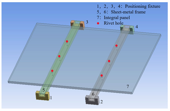
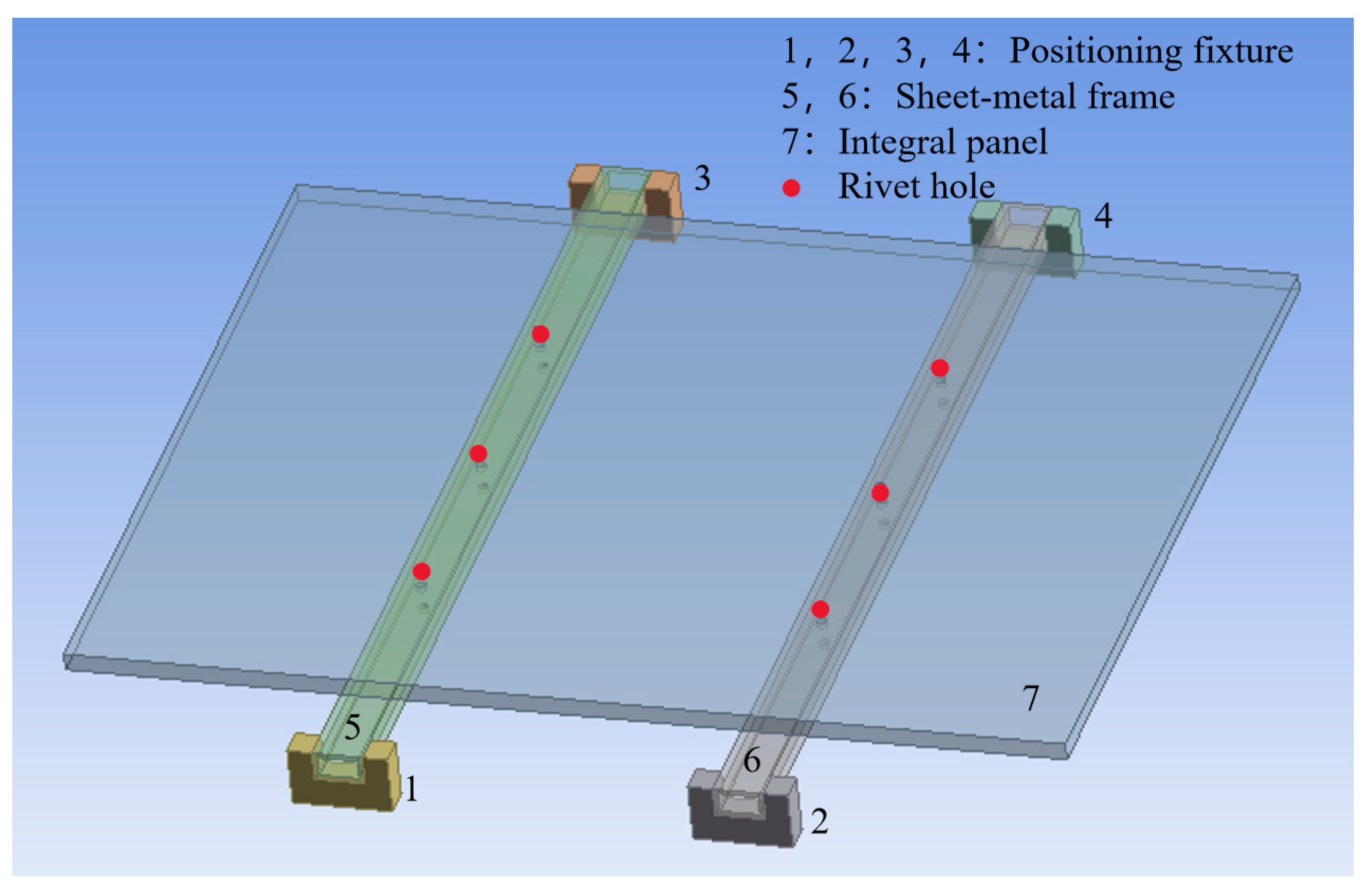
To evaluate the noise robustness of the proposed KW-PEAH method in a controlled engineering setting, a thin-walled assembly consisting of an integral panel and two sheet-metal frames is considered (Figure 2). The overall dimensions are 1000 mm × 800 mm × 18 mm. The integral panel is made of aluminum alloy, with a nominal elastic modulus of E = 75 GPa, a nominal Poisson’s ratio of ν = 0.33, and a density of 2770 kg/m³.

Figure 2. Structural model of the thin-walled parts.

Finite element analysis is performed using ANSYS Workbench 2024 R2. The integral panel was modeled using three-dimensional solid elements. The final mesh contained 57,957 nodes and 30,195 solid finite elements, including 29,155 Tet10 elements, 832 Hex20 elements, and 208 Pyramid13 elements. The assembly procedure for the entire component is as follows: the sheet-metal frames are first mounted onto the positioning tooling, and then the integral panel is placed over the frames and joined to them by riveting at six rivet holes.

Deviation considerations: The manufacturing deviations are mainly manifested as the z-directional manufacturing deviations of the sheet-metal frames, with a tolerance range of [0, +1.5 mm]; the material property deviations include the elastic modulus deviation range of [69, 81] GPa and the Poisson’s ratio deviation range of [0.3036, 0.3564]. These constitute three input variables, while the output variable is the mean y-directional displacement deformation of the panel. For simplicity, it is assumed here that the sheet-metal frames transfer the deviations to the integral panel through the six rivet points. To construct a controlled simulation-based dataset, all input deviations are assumed to be mutually independent in the present finite element model.

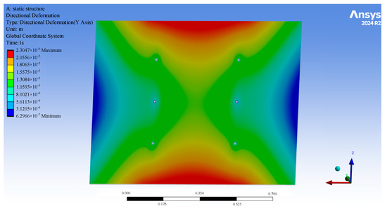
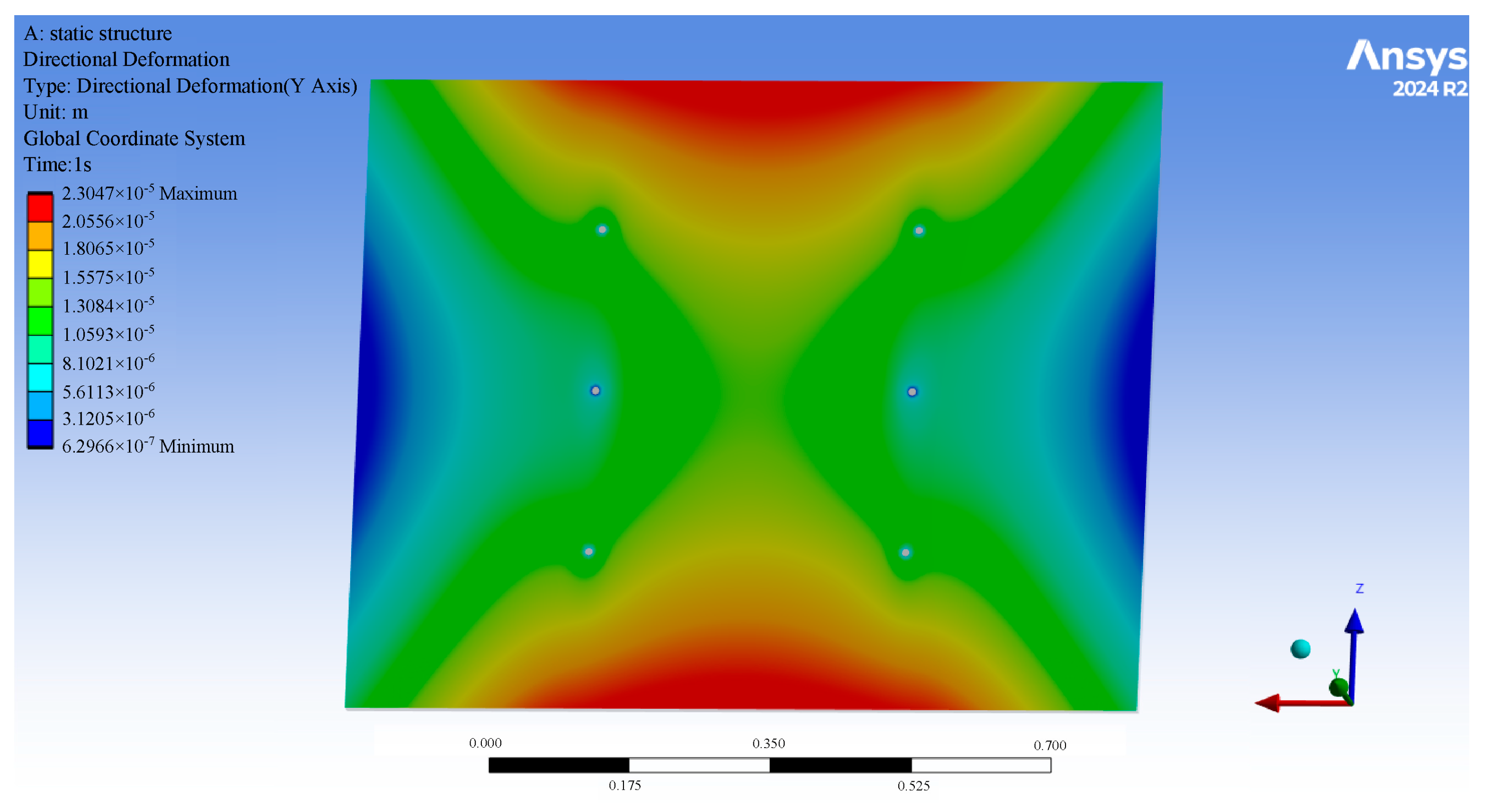
Figure 3 shows a typical finite element analysis result. The procedure for this case is as follows:

Figure 3. A typical finite element analysis result of one sample.

(1)

A total of 300 sample points are generated using Latin hypercube sampling (LHS), and the corresponding responses are obtained through finite-element simulations.

(2)

The dataset is divided into 70% training and 30% testing sets using a sequential maximin-distance sampling strategy.

(3)

Controlled noise at three levels (5%, 10%, and 15%) is added only to the training responses in the form of zero-mean Gaussian perturbations, with standard deviations proportional to those of the original responses. The test set remains noise-free.

(4)

The input and output variables are standardized using Z-score normalization. The standardization parameters are calculated from the training set and applied to both the training and testing sets. The noisy training responses are standardized using the mean and standard deviation of the original training responses.

(5)

Each base model is trained on the noisy training set. Hyperparameters are tuned by Bayesian optimization, and pointwise cross-validation errors are estimated via 5-fold cross-validation.

(6)

The trained base models are combined under different ensemble strategies.

(7)

The ensemble predictions are transformed back to the original scale, and RMSE, MAE, and R² are calculated using the noise-free testing responses.

(8)

20 independent trials are conducted at each noise level using different data partitions and noise realizations.

This experimental design provides a controlled and reproducible framework for evaluating the accuracy and noise robustness of the six ensemble strategies. The corresponding results are presented and analyzed in Section 4.2.

3.3. Evaluation Metrics

The Root Mean Square Error (RMSE) reflects the overall dispersion level of prediction errors and is highly sensitive to larger errors. The Mean Absolute Error (MAE) represents the average level of absolute deviations between predicted and true values, intuitively indicating the average prediction accuracy of the model. The Coefficient of Determination (R²) measures the goodness of fit between the model predictions and the true responses. Since the numerical values of RMSE and MAE vary across different test problems, this paper adopts the Normalized Root Mean Square Error (NRMSE) and the Normalized Mean Absolute Error (NMAE) as alternative metrics for the test function part [35]. Their calculation formulas are given as follows:

$$R^2=1-{\displaystyle \frac{{\displaystyle {\sum }_{i=1}^K{\left(y_i-{\widehat{y}}_i\right)}^2}}{{\displaystyle {\sum }_{i=1}^K{\left(y_i-\overline{y}\right)}^2}}}$$

(25)

$$\mathit{RMSE}=\sqrt{{\displaystyle \frac{1}{K}}{\displaystyle \sum _{i=1}^K{\left(y_i-{\widehat{y}}_i\right)}^2}},\mathit{NRMSE}=\sqrt{{\displaystyle {\sum }_{i=1}^K{\left(y_i-{\widehat{y}}_i\right)}^2}/{\displaystyle {\sum }_{i=1}^K{y_i}^2}}$$

(26)

$$\mathit{MAE}={\displaystyle \frac{1}{K}}{\displaystyle {\sum }_{i=1}^K\left|y_i-{\widehat{y}}_i\right|},\mathit{NMAE}={\displaystyle \frac{1}{K}}{\displaystyle {\sum }_{i=1}^K\left|y_i-{\widehat{y}}_i\right|}/\sqrt{{\displaystyle \frac{1}{K}}{\displaystyle {\sum }_{i=1}^K{\left(y_i-\overline{y}\right)}^2}}$$

(27)

where K is the total number of test sample points, y_i is the true response value of the ith test sample, ${\widehat{y}}_i$ is the predicted response value of the ith test sample, and $\overline{y}$ is the mean of the true response values of all test samples.

3.4. Parameter Sensitivity Analysis

The parameters in Equation (12) of the KW-PEAH method, the number of nearest neighbors k and the adjustment coefficient c have a direct impact on the value of the kernel bandwidth h(x). To determine a reasonable parameter configuration, this section, based on the experience from the literature [39], takes the RMSE of the thin-walled parts assembly deviation analysis case under a 10% noise level as the evaluation metric, fixes other parameters (such as α and β), and conducts a sensitivity analysis on k and c. The value range of k is [3, 4, 5, 6, 7], and the value range of c is [0.3, 0.4, 0.5, 0.6, 0.7]. The results are shown in Table 2. The optimal values are marked in bold, and the same formatting is applied to the following tables.

Table 2. Comparison of average RMSE (×10⁻⁵ m) for different parameter combinations.

c\k	3	4	5	6	7
0.3	4.5963	4.5955	4.5942	4.5928	4.5924
0.4	4.5989	4.5976	4.5971	4.5964	4.5968
0.5	4.6034	4.6040	4.6054	4.6058	4.6075
0.6	4.6110	4.6131	4.6154	4.6168	4.6197
0.7	4.6193	4.6219	4.6243	4.6265	4.6306

As shown in Table 2, when k = 7 and c = 0.3, the RMSE reaches its minimum value of 4.59 × 10⁻⁵; when k = 7 and c = 0.7, the RMSE reaches its maximum value of 4.63 × 10⁻⁵, with a maximum fluctuation difference of 0.83%.

It should be noted that the parameter sensitivity analysis was conducted only for the thin-walled assembly case under the 10% noise condition; therefore, the selected configuration is not claimed to be universally optimal for all benchmark functions.

It can be observed that regardless of how k and c are combined, the performance of the KW-PEAH algorithm consistently converges within a relatively narrow range, indicating that KW-PEAH is relatively insensitive to k and c within the examined ranges. This low sensitivity suggests that applying the selected parameter configuration to different problems is unlikely to cause substantial performance degradation. Considering the balance between the kernel bandwidth and the local neighborhood range, intermediate values of k = 5 and c = 0.5 are adopted as the default parameter configuration for all subsequent experiments. Future work will investigate automatic parameter-tuning strategies for different dimensions and response-surface characteristics.

3.5. Sensitivity Analysis of Base Surrogate Model Composition

To investigate the robustness of the proposed ensemble strategies with respect to the composition of base surrogate models, a leave-one-out sensitivity analysis was conducted. Specifically, each of the six base models (PRS, Kriging, RBF, SVR, ANN, and RF) was removed in turn, and the ensemble methods were reconstructed using the remaining five models. The results are compared with those obtained using the full set of base models.

Table 3 presents the leave-one-out sensitivity analysis of the base surrogate model composition under a 10% noise level. Across the complete and reduced base model combinations, KW-PEAH consistently achieves lower RMSE values than the corresponding PEAH models. Furthermore, after removing any one of the base surrogate models, the RMSE range of KW-PEAH fluctuates by approximately 5.6%, whereas the corresponding fluctuation range for PEAH is approximately 10.9%. These results suggest that KW-PEAH is less sensitive to the composition of the base-surrogate-model pool and can maintain relatively stable prediction performance even when the pool is reduced. This finding further indicates that the adaptive Gaussian kernel weighting mechanism can, to some extent, alleviate the performance fluctuations caused by removing individual base surrogate models.

Table 3. Comparison of average RMSE (×10⁻⁵ m) for sensitivity analysis of base surrogate model.

	ALL	Without PRS	Without Kriging	Without RBF	Without SVR	Without ANN	Without RF
PEAH	4.6284	4.9833	5.1368	4.2865	4.9806	4.4415	4.4442
KW-PEAH	4.2944	4.5071	4.5320	4.2721	4.5003	4.0785	4.3561

It should also be noted that including more base surrogate models does not necessarily guarantee better ensemble performance, since some models may provide redundant or noise-sensitive predictions under specific conditions. Moreover, the leave-one-out sensitivity analysis was conducted under the representative 10% noise condition, using the same data partition and noise realization for all base-model configurations, rather than independently generating datasets for each configuration. Therefore, the results are intended as a controlled comparison of KW-PEAH’s sensitivity to changes in the base-surrogate-model composition, not as an independent assessment of its performance across all noise conditions.

4. Experimental Comparison Results

4.1. Comparison on Test Functions

In this section, six ensemble strategies are systematically compared using eight classical test functions. The same six base models (PRS, Kriging, RBF, SVR, ANN, and RF) are integrated in all strategies to ensure a fair comparison. Table 4, Table 5 and Table 6 present the mean values of NRMSE, NMAE, and R², respectively. The corresponding standard deviations and 95% confidence intervals are provided in the Supplementary Material. In addition, a two-sided Wilcoxon signed-rank test was performed to assess the statistical significance of the differences between KW-PEAH and PEAH, and the corresponding p-values are reported in Table 7.

Table 4. Comparison of NRMSE values.

	BH	CB	GF	HN3	SK	HN6	ER	DP
UA	0.5491	0.8065	0.7712	0.4871	0.7336	0.7943	0.4784	0.5077
IRMSE	0.4922	0.7738	0.6850	0.4670	0.7126	0.7784	0.4567	0.4623
BA	0.4802	0.7648	0.6611	0.4735	0.7093	0.7651	0.4637	0.4707
OWPE	0.5431	0.7912	0.6695	0.4585	0.7109	0.7641	0.4640	0.4481
PEAH	0.5108	0.7558	0.6606	0.4507	0.6863	0.7623	0.4538	0.4312
KW-PEAH	0.4791	0.7457	0.6589	0.4616	0.6925	0.7572	0.4406	0.4438

Table 5. Comparison of NMAE values.

	BH	CB	GF	HN3	SK	HN6	ER	DP
UA	0.3684	0.5125	0.4578	0.3441	0.4553	0.4848	0.3717	0.3982
IRMSE	0.3220	0.4828	0.3562	0.3265	0.4298	0.4765	0.3544	0.3604
BA	0.3127	0.4846	0.3170	0.3326	0.4254	0.4725	0.3599	0.3674
OWPE	0.3600	0.5099	0.3399	0.3094	0.3782	0.4848	0.3502	0.3568
PEAH	0.3136	0.4721	0.3259	0.3128	0.3521	0.4611	0.3551	0.3448
KW-PEAH	0.2971	0.4637	0.3226	0.3251	0.3634	0.4531	0.3428	0.3582

Table 6. Comparison of R² values.

	BH	CB	GF	HN3	SK	HN6	ER	DP
UA	0.5158	0.4418	0.4507	0.7605	0.4536	0.3864	0.7704	0.7411
IRMSE	0.6710	0.4966	0.4996	0.7891	0.4863	0.4016	0.7909	0.7854
BA	0.7034	0.5011	0.5151	0.7631	0.4915	0.4166	0.7845	0.7774
OWPE	0.5812	0.3693	0.4702	0.7757	0.4880	0.3937	0.8041	0.7797
PEAH	0.7208	0.5125	0.5483	0.8226	0.5273	0.4164	0.7989	0.8079
KW-PEAH	0.7531	0.5199	0.5504	0.7845	0.5194	0.4389	0.8032	0.8025

Table 7. p-Value of two-sided Wilcoxon signed-rank test results comparing KW-PEAH and PEAH on the eight benchmark functions.

	BH	CB	GF	HN3	SK	HN6	ER	DP
NRMSE	1.17 × 10−3	2.17 × 10−5	3.80 × 10−5	0.783	0.877	7.18 × 10−9	4.92 × 10−3	6.77 × 10−6
NMAE	2.19 × 10−3	2.84 × 10−3	1.29 × 10−3	0.812	0.127	2.37 × 10−12	2.06 × 10−3	1.43 × 10−6
R2	2.34 × 10−3	2.69 × 10−5	3.13 × 10−5	0.799	0.872	5.97 × 10−9	4.76 × 10−3	6.45 × 10−6

The comparison results on eight classical benchmark functions, as shown in Table 4, Table 5 and Table 6, indicate that KW-PEAH exhibits good performance on the three core evaluation metrics for most test functions. In terms of NRMSE, this method achieves better test results on BH (0.4791), CB (0.7457), GF (0.6589), HN6 (0.7572), and ER (0.4406), outperforming the other compared ensemble methods. In terms of NMAE, KW-PEAH achieves the lowest values among the six methods on BH (0.2971), CB (0.4637), HN6 (0.4531), and ER (0.3428). In terms of R², this method outperforms PEAH and most of the compared methods on BH (0.7531), CB (0.5199), GF (0.5504), HN6 (0.4389), and ER (0.8032). Therefore, the advantages of KW-PEAH are mainly reflected in functions with smooth, continuous, ridge-shaped or valley-shaped response surfaces (e.g., BH, ER) as well as high-dimensional sparse functions (e.g., HN6, ER). In these cases, the smoothing property of the Gaussian kernel, together with the adaptive bandwidth mechanism, helps stabilize local estimation and improve prediction accuracy.

Nevertheless, the improvement is not consistent across all response surfaces. For multimodal functions with sharp local features, such as SK, Gaussian kernel weighting may excessively smooth local peaks and valleys, thereby weakening the model’s ability to capture sharp response variations and causing smoothing-induced bias.

For the Hartmann-type response surfaces considered in this study, the effectiveness of Gaussian kernel weighting depends on the response-surface characteristics. On HN3, KW-PEAH yields an NRMSE of 0.4616, compared with 0.4507 for PEAH, with a difference of approximately 2.42%. One possible explanation is that Gaussian kernel weighting may excessively smooth localized exponential contributions, thereby weakening informative local variations in the cross-validation-error field. In contrast, the higher dimensionality and sparse sampling of HN6 make the original distance-based weighting more sensitive to individual samples. As a result, KW-PEAH exhibits different performances on these two functions.

Furthermore, the results for the 12-dimensional DP function indicate that the proposed Gaussian-kernel smoothing method is not universally beneficial for high-dimensional problems with strongly coupled, chain-dependent variables. One possible reason is that smoothing may weaken local error variations that are important for representing variable interactions. Further studies are needed to distinguish the effects of different factors.

Table 7 presents the results of the two-sided Wilcoxon signed-rank test comparing KW-PEAH with PEAH across the eight benchmark functions. At the significance level of 0.05, statistically significant differences are observed for all three metrics on BH, CB, GF, HN6 and ER (p < 0.05). In contrast, no statistically significant difference is detected for HN3 or SK (p > 0.05), which suggests that the performance difference between KW-PEAH and PEAH is not statistically distinguishable on these two functions under the present experimental settings. When interpreted jointly with Table 4, Table 5 and Table 6, the results support the effectiveness of KW-PEAH on several benchmark functions, while also confirming that its advantage depends on the dimensionality and local characteristics of the response surface.

Overall, KW-PEAH achieves better or comparable predictive performance to the original PEAH on most of the benchmark functions examined. However, its performance is not uniformly superior across all cases, as its effectiveness depends on the dimensionality and local characteristics of the response surface. Thus, the results demonstrate problem-dependent advantages rather than universal superiority.

4.2. Comparison on the Simulation Case

To provide a structured evaluation of the simulation case, this section is divided into two parts. Section 4.2.1 evaluates the predictive performance of the ensemble strategies using the mean values, boxplot distributions, and results of the two-sided Wilcoxon signed-rank test. Section 4.2.2 compares the computational costs of PEAH and KW-PEAH, with particular attention to parameter-optimization and prediction times.

4.2.1. Predictive Performance and Statistical Comparison

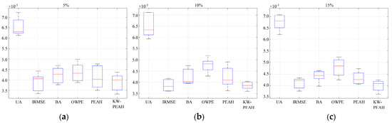
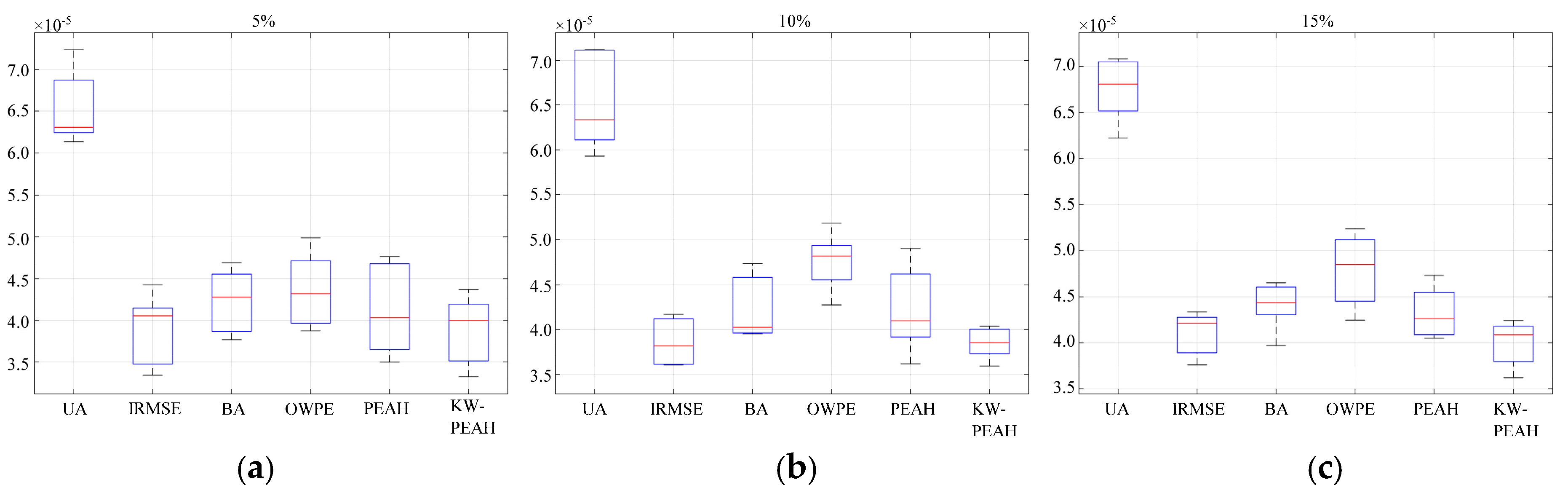
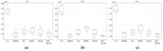
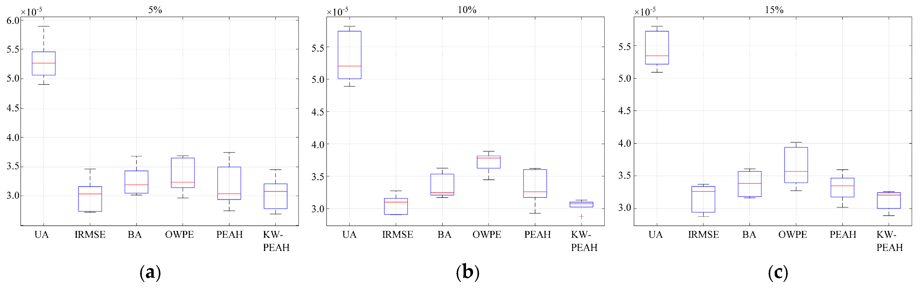
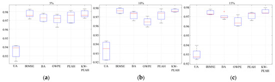
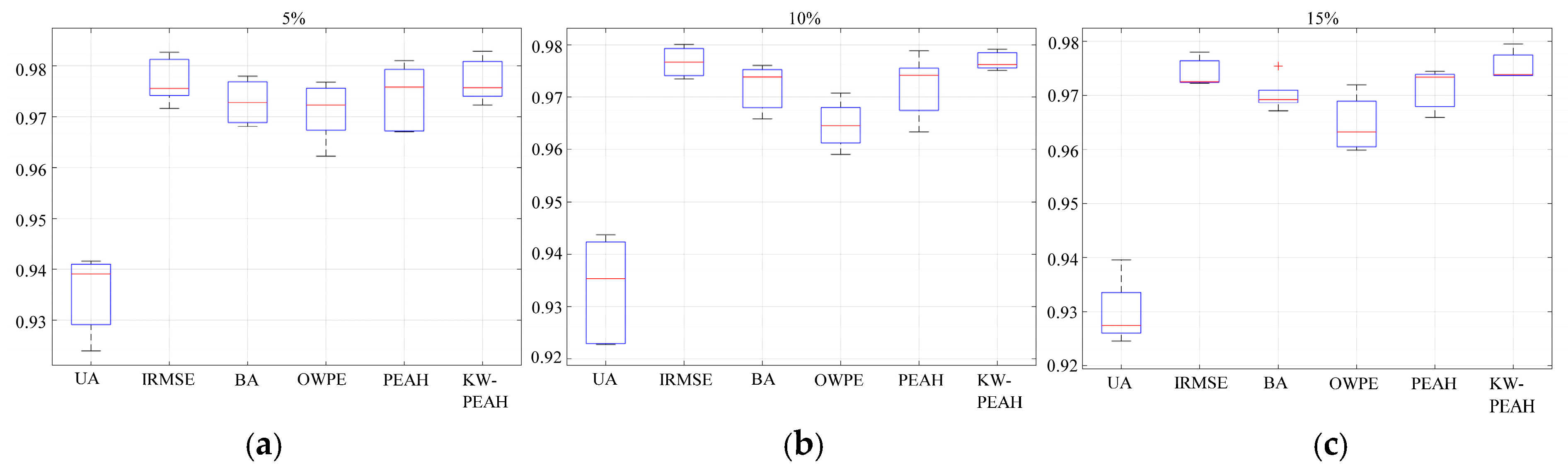
This section compares the six ensemble strategies using the same six base surrogate models. Table 8, Table 9 and Table 10 report the mean RMSE, MAE, and R² values under the three noise levels, while Figure 4, Figure 5 and Figure 6 present the corresponding boxplots to illustrate the distributions of these metrics across the independent trials. To further assess the statistical significance of the performance differences between KW-PEAH and PEAH, a two-sided Wilcoxon signed-rank test was conducted using the paired results from the 20 independent trials at each noise level, and the corresponding p-values are reported in Table 11.

Table 8. Mean RMSE values (×10⁻⁵) of the six ensemble strategies under three noise levels.

	UA	IRMSE	BA	OWPE	PEAH	KW-PEAH
5%	6.6155	3.9236	4.3752	4.3923	4.1186	3.9252
10%	6.8058	4.0690	4.2165	4.7003	4.2163	3.9321
15%	6.7352	4.1815	4.4961	4.8578	4.2936	4.1217

Table 9. Mean values of MAE (×10⁻⁵) of the six ensemble strategies under three noise levels.

	UA	IRMSE	BA	OWPE	PEAH	KW-PEAH
5%	5.2784	2.9525	3.2388	3.4655	3.2783	3.0414
10%	5.4078	3.0847	3.3587	3.6859	3.2692	3.0863
15%	5.4008	3.2581	3.3578	3.7283	3.3422	3.1909

Table 10. Mean values of R² of the six ensemble strategies under three noise levels.

	UA	IRMSE	BA	OWPE	PEAH	KW-PEAH
5%	0.9357	0.97907	0.9734	0.9714	0.9742	0.9775
10%	0.9379	0.97628	0.9714	0.9658	0.9719	0.9793
15%	0.9307	0.97294	0.9692	0.96281	0.9705	0.9772

Figure 4. Comparison of RMSE values. (a) 5% noise level; (b) 10% noise level; (c) 15% noise level.

Figure 5. Comparison of MAE values. (a) 5% noise level; (b) 10% noise level; (c) 15% noise level.

Figure 6. Comparison of R² values. (a) 5% noise level; (b) 10% noise level; (c) 15% noise level.

Table 11. p-Value of two-sided Wilcoxon signed-rank test results comparing KW-PEAH and PEAH on the thin-walled parts case.

	RMSE	MAE	R2
5	6.9 × 10−5	1.7 × 10−3	6.9 × 10−5
10	1.8 × 10−5	4.9 × 10−5	1.8 × 10−5
15	6.9 × 10−5	1.5 × 10−5	6.3 × 10−5

As shown in Table 8, Table 9 and Table 10, KW-PEAH achieves lower mean RMSE and MAE than PEAH at all three noise levels. Specifically, the mean RMSE is reduced by approximately 4.00–6.74%, while the mean MAE is reduced by approximately 4.53–7.23%. KW-PEAH also achieves higher mean R² values than PEAH under all noise conditions, with the improvement being particularly evident at the 10% and 15% noise levels. These results may be attributed to the smooth distance-decay mechanism of Gaussian kernel weighting, which reduces the excessive influence of individual noisy samples on the local ensemble weights.

The boxplots in Figure 4, Figure 5 and Figure 6 further illustrate the performance distributions of PEAH and KW-PEAH. Overall, the RMSE and MAE distributions of KW-PEAH are generally lower than those of PEAH, while its R² distributions are generally higher, particularly under the 10% and 15% noise levels. Meanwhile, the comparatively compact interquartile ranges of KW-PEAH indicate relatively small performance fluctuations across different trials. These distributional characteristics are consistent with the mean results, suggesting that the improvements are not caused by a few favorable trials but are generally maintained across different data partitions and noise realizations.

As shown in Table 11, all p-values are lower than 0.05. The results indicate that the performance differences observed between the two methods are statistically significant, rather than being caused only by random variations among the independent trials.

When considered together with the mean values and boxplot results, these statistical findings support the effectiveness of KW-PEAH in reducing prediction errors and maintaining a higher goodness of fit than PEAH in this simulation case. This improvement is consistent with the intended effect of Gaussian kernel weighting and KNN-based adaptive bandwidth adjustment.

4.2.2. Computational Cost Analysis

To evaluate the computational efficiency of the ensemble strategies, the average parameter-optimization time and prediction time of PEAH and KW-PEAH were measured under three noise levels. The results are presented in Table 12:

Table 12. Comparison of average computational time between PEAH and KW-PEAH.

Noise Level	Method	Optimization Time (s)	Prediction Time (s)	Total Increase
5%	PEAH	169.66	1.69	+29.7%
	KW-PEAH	220.56	1.70
10%	PEAH	162.44	1.42	+11.2%
	KW-PEAH	180.85	1.43
15%	PEAH	185.72	1.74	+8.2%
	KW-PEAH	201.18	1.72

The results clearly show that the additional computational cost of KW-PEAH mainly arises from the optimization of the weighting parameters. Once these parameters are determined, the prediction time difference between KW-PEAH and PEAH is negligible. The relative runtime overhead decreases from 29.7% at the 5% noise level to 8.2% at the 15% noise level. Although KW-PEAH requires additional optimization time, the overhead is small compared with the training time of the base surrogate models or the cost of finite element analysis.

Overall, the simulation results for the thin-walled assembly demonstrate that KW-PEAH achieves a favorable balance among prediction accuracy, noise robustness, and computational cost. Therefore, KW-PEAH is effective for the present low-dimensional thin-walled assembly-deviation problem under noisy conditions.

It should also be emphasized that the simulation engineering case demonstrates the relative noise robustness of KW-PEAH under the three-variable finite-element setting. However, its general applicability to high-dimensional or real-world assembly cases requires further validation in future work.

5. Conclusions

This paper addresses the accuracy and robustness limitations of ensemble surrogate models for thin-walled assembly-deviation analysis. To improve the continuity and local adaptability of the PEAH weighting mechanism, a kernel-weighted pointwise ensemble method, termed KW-PEAH, was developed by combining Gaussian kernel weighting with a KNN-based adaptive bandwidth strategy. The proposed method was systematically compared with UA, IRMSE, BA, OWPE, and PEAH using eight benchmark functions and a simulation-based thin-walled assembly case with three levels of noise. Its prediction accuracy, robustness, and computational efficiency were systematically evaluated.

The experimental results show that KW-PEAH achieves lower errors or comparable performance to the competing methods on most benchmark functions. Compared with PEAH, KW-PEAH reduces the mean NRMSE by approximately 6.21% and 2.91% on the BH and ER functions, respectively. In the thin-walled assembly case, KW-PEAH reduces the mean RMSE by 4.00–6.74% and the mean MAE by 4.53–7.23% across the three noise levels. The two-sided Wilcoxon signed-rank tests confirm that the differences are statistically significant, providing evidence of improved predictive performance in the presence of training noise. Although the additional bandwidth calculation introduces a modest computational overhead, KW-PEAH provides a potentially useful surrogate-modelling approach for low- to medium-dimensional thin-walled assembly-deviation analysis under noisy conditions.

Nevertheless, the smoothing effect of Gaussian kernel weighting is not universally advantageous. The method may underperform on response surfaces with sharp local peaks or abrupt local variations because Gaussian smoothing can introduce bias. Future work will explore boundary-correction and hybrid-kernel strategies to mitigate the excessive smoothing of sharp local peaks, thereby improving the effectiveness and applicability of the proposed method.

Another limitation is that this thin-walled case study relies solely on finite element simulations with three input variables. Consequently, the present case represents a controlled low-dimensional scenario and does not establish the effectiveness of KW-PEAH for high-dimensional engineering applications. Furthermore, the finite element model assumes that geometric and material deviations are independent and has not been validated against physical experiments, whereas such deviations are often coupled in practical applications. Future work will incorporate higher-fidelity multiphysics simulations, physical experiments, and coupling-aware approaches (e.g., multivariate Gaussian processes, copula-based sampling, and physics-informed neural networks) together with dimension- and interaction-aware bandwidth selection.

References

- Han, X.; Shi, F.; Zhuang, W.; Hua, L.; Zheng, F.; Xu, M. A novel multi-DOF point envelope forming process for manufacturing thin-walled components. J. Manuf. Process. 2025, 134, 1082–1095. [Google Scholar] [CrossRef] [Scilit]
- Gao, C.; Yu, H. Modeling of random field deviation and assembled geometrical accuracy for large thin-walled structures. Robot. Intell. Autom. 2025, 45, 614–627. [Google Scholar] [CrossRef] [Scilit]
- Miller, B.; Ziemiański, L. Multi-Objective Optimization of Thin-Walled Composite Axisymmetric Structures Using Neural Surrogate Models and Genetic Algorithms. Materials 2023, 16, 6794. [Google Scholar] [CrossRef] [Scilit] [PubMed]
- Tang, J.; Deng, C.; Chen, X.; Zhai, H. Analysis and Optimization of Milling Deformations of TC4 Alloy Thin-Walled Parts Based on Finite Element Simulations. Machines 2023, 11, 628. [Google Scholar] [CrossRef] [Scilit]
- Yue, C.; Jia, R.; Zhu, X.; Geng, B.; Zhang, J. Research on online deformation monitoring of thin-walled parts driven by digital twin. Digit. Eng. 2024, 3, 100023. [Google Scholar] [CrossRef] [Scilit]
- Yu, G.K.; Yang, H.Z. Assembly variation modeling method research of compliant automobile body sheet metal parts using the finite element method. Int. J. Automot. Technol. 2015, 16, 51–56. [Google Scholar] [CrossRef] [Scilit]
- Wollaber, B.A. Four Decades of Implicit Monte Carlo. J. Comput. Theor. Transp. 2016, 45, 1–70. [Google Scholar] [CrossRef] [Scilit]
- Boyuan, P.; Xianming, W.; Tianxiao, Z. Reliability analysis of thin-walled ring gear based on tooth surface fatigue and wear. J. Mech. Sci. Technol. 2024, 38, 1985–1997. [Google Scholar] [CrossRef] [Scilit]
- Homem, T.; Bayraksan, G. Monte Carlo sampling based methods for stochastic optimization. Surv. Oper. Res. Manag. Sci. 2014, 19, 56–85. [Google Scholar] [CrossRef] [Scilit]
- Polini, W.; Corrado, A. Methods of influence coefficients to evaluate stress and deviation distribution of flexible assemblies—A review. Int. J. Adv. Manuf. Technol. 2020, 107, 2901–2915. [Google Scholar] [CrossRef] [Scilit]
- Lindau, B.; Lorin, S.; Lindkvist, L.; Söderberg, R. Efficient Contact Modeling in Nonrigid Variation Simulation. J. Comput. Inf. Sci. Eng. 2016, 16, 011002. [Google Scholar] [CrossRef] [Scilit]
- Maltauro, M.; Passarotto, G.; Concheri, G.; Meneghello, R. Bridging the gap between design and manufacturing specifications for non-rigid parts using the influence coefficient method. Int. J. Adv. Manuf. Technol. 2023, 127, 579–597. [Google Scholar] [CrossRef] [Scilit]
- Tian, X.X.; Wan, C.H.; Duan, F.; Wu, D.; Chang, L.; Nie, X.H. Physics-informed deep operator network for bending analysis of stiffened panels. Thin-Walled Struct. 2026, 225, 114765. [Google Scholar] [CrossRef] [Scilit]
- Sun, H.R.; Lin, L.; Jiang, L.B.; Zheng, S.G.; Wang, Q.; Ke, Y.L. A manifold learning-assisted generative adversarial network for rapid assembly stress field prediction in complex composite aircraft panels. Thin-Walled Struct. 2026, 226, 114962. [Google Scholar] [CrossRef] [Scilit]
- Yan, J.H.; Ding, H.Q. A hybrid rigid-compliant computational framework for large-scale assembly: Integrating torsor kinematics with physics-informed graph learning. Eng. Struct. 2026, 362, 122965. [Google Scholar] [CrossRef] [Scilit]
- Serani, A.; Scholcz, T.P.; Vanzi, V. A Scoping Review on Simulation-Based Design Optimization in Marine Engineering: Trends, Best Practices, and Gaps. Arch. Comput. Methods Eng. 2024, 31, 4709–4737. [Google Scholar] [CrossRef] [Scilit] [PubMed]
- Xue, D.; Li, Y.; Zhang, H.; Tong, X.; Gao, B.; Yu, J. Reliability-based robust optimization design for tolerance of aerospace thin-walled components based on surrogate model. Adv. Eng. Inform. 2024, 62, 102754. [Google Scholar] [CrossRef] [Scilit]
- Viana, F.A.C.; Haftka, R.T. Using Multiple Surrogates for Metamodeling. In Proceedings of the 7th ASMO-UK/ISSMO International Conference on Engineering Design Optimization, Bath, UK, 7–8 July 2008. [Google Scholar]
- Ravikumar, A.; Periyasamy, V.; Devi, K.M.K.; Krishnamoorthy, R.G.; Mariavalavan, O.K. A hybrid SERWI ensemble model for crop yield prediction using an inverse RMSE weighting strategy. Sci. Rep. 2025, 15, 45085. [Google Scholar] [CrossRef] [Scilit] [PubMed]
- Hu, J.; Peng, Y.; Lin, Q.; Liu, H.; Zhou, Q. An ensemble weighted average conservative multi-fidelity surrogate modeling method for engineering optimization. Eng. Comput. 2020, 38, 2221–2244. [Google Scholar] [CrossRef] [Scilit]
- Lu, J.; Fang, Y.; Han, W. A novel adaptive-weight ensemble surrogate model base on distance and mixture error. PLoS ONE 2023, 18, e0293318. [Google Scholar] [CrossRef] [Scilit] [PubMed]
- Zhao, C.; Lin, C.; Wang, F.; Qi, H.; Li, Z.; Li, T.; He, Y. Time-variant deformation prediction and reliability assessment of slopes based on dynamic Bayesian model averaging. Eng. Geol. 2026, 365, 108647. [Google Scholar] [CrossRef] [Scilit]
- Li, Z.; Yang, Z.; Teng, L.; Xie, S.; Tian, M. Machine-learning ensembled probabilistic methods for time-dependent reliability analysis of reservoir slopes under rapid water level drawdown using Bayesian model averaging (BMA). Sci. Rep. 2025, 15, 43776. [Google Scholar] [CrossRef] [Scilit] [PubMed]
- Lee, Y.; Choi, D. Pointwise ensemble of meta-models using v nearest points cross-validation. Struct. Multidiscip. Optim. 2014, 50, 383–394. [Google Scholar] [CrossRef] [Scilit]
- Liu, H.; Xu, S.; Wang, X.; Meng, J.; Yang, S. Optimal Weighted Pointwise Ensemble of Radial Basis Functions with Different Basis Functions. AIAA J. 2016, 54, 3117–3133. [Google Scholar] [CrossRef] [Scilit]
- Chen, H.; Li, W.; Cui, W.; Liu, Q. A pointwise ensemble of surrogates with adaptive function and heuristic formulation. Struct. Multidiscip. Optim. 2022, 65, 113. [Google Scholar] [CrossRef] [Scilit]
- Yang, Y.; Yang, Y.; Xiao, M.; Wan, M.; Zhang, W. A Gaussian process regression-based surrogate model of the varying workpiece dynamics for chatter prediction in milling of thin-walled structures. Int. J. Mech. Syst. Dyn. 2022, 2, 117–130. [Google Scholar] [CrossRef] [Scilit]
- Zhou, Y.; Lu, Z.; Cheng, K. A new surrogate modeling method combining polynomial chaos expansion and Gaussian kernel in a sparse Bayesian learning framework. Int. J. Numer. Methods Eng. 2019, 120, 498–516. [Google Scholar] [CrossRef] [Scilit]
- Wang, H.; Li, P.; Ai, M.; Wu, J.; Yang, C.; Pan, D. Gaussian-kernel weighted neighborhood preserving embedding algorithm and its application in fault detection. Meas. Sci. Technol. 2024, 35, 086207. [Google Scholar] [CrossRef] [Scilit]
- Zhu, Y.G.; Shi, Q.; Jiang, W.P.; Deng, B. Key deviation source diagnosis of complex thin-walled structures based on complex networks and weighted transfer entropy. Aeronaut. J. 2024, 128, 812–829. [Google Scholar] [CrossRef] [Scilit]
- Gao, W.; Oh, S.; Viswanath, P. Density Functional Estimators with k-Nearest Neighbor Bandwidths. In Proceedings of the 2017 IEEE International Symposium on Information Theory (ISIT); IEEE: New York, NY, USA, 2017. [Google Scholar]
- Cover, T.; Hart, P. Nearest neighbor pattern classification. IEEE Trans. Inf. Theory 2003, 13, 21–27. [Google Scholar]
- Patil, M.D.; Sarate, G.G. Optimum adaptive bandwidth selection method of local fitting in kernel regression analysis for non-uniform data. Signal Image Video Process. 2023, 17, 3347–3358. [Google Scholar] [CrossRef] [Scilit]
- Xia, J.; Wanli, Y.; Sheng, P.Y. Adaptive active learning through k-nearest neighbor optimized local density clustering. Appl. Intell. 2023, 53, 14892–14902. [Google Scholar] [CrossRef] [Scilit]
- Ye, P.; Pan, G. Selecting the Best Quantity and Variety of Surrogates for an Ensemble Model. Mathematics 2020, 8, 1721. [Google Scholar] [CrossRef] [Scilit]
- Loftsgaarden, D.O.; Quesenberry, C.P. A Nonparametric Estimate of a Multivariate Density Function. Ann. Math. Stat. 1965, 36, 1049–1051. [Google Scholar] [CrossRef] [Scilit]
- Talgorn, B.; Le Digabel, S.; Kokkolaras, M. Statistical Surrogate Formulations for Simulation-Based Design Optimization. J. Mech. Des. 2015, 137, 021405. [Google Scholar] [CrossRef] [Scilit]
- Zhang, J.; Yue, X.; Qiu, J.; Zhang, M.; Wang, X. A unified ensemble of surrogates with global and local measures for global metamodelling. Eng. Optim. 2021, 53, 474–495. [Google Scholar] [CrossRef] [Scilit]
- Yang, Y. An Evaluation of Statistical Approaches to Text Categorization. Inf. Retr. 1999, 1, 69–90. [Google Scholar] [CrossRef] [Scilit]
Disclaimer/Publisher’s Note: The statements, opinions and data contained in all publications are solely those of the individual author(s) and contributor(s) and not of MDPI and/or the editor(s). MDPI and/or the editor(s) disclaim responsibility for any injury to people or property resulting from any ideas, methods, instructions or products referred to in the content. |
© 2026 by the authors. Licensee MDPI, Basel, Switzerland. This article is an open access article distributed under the terms and conditions of the Creative Commons Attribution (CC BY) license.