An Approximate Force–Indentation Equation for n-Sided Blunt Pyramidal Indenters

Abstract

Accurate AFM nanoindentation analysis requires models that account for the rounded apex of real pyramidal indenters. Although exact force-indentation equations for n-sided blunt pyramids exist, their numerical complexity limits routine use. In this work, a simple closed-form analytical approximation is developed that directly relates force to indentation depth for blunt pyramidal indenters. The method employs first-order Maclaurin series expansions of the geometric terms and the generic indentation differential equation, yielding a closed-form second-degree polynomial expression that is readily implemented in AFM data analysis. Comparison with the exact solutions showed that the approximation error decreases with indentation depth and is governed by the pyramid geometry rather than the tip radius. Simulated and experimental AFM data confirmed accurate Young’s modulus estimation above a geometry-dependent validity threshold. For a four-sided blunt pyramidal indenter, the proposed criterion predicts minimum indentation depths ranging from approximately $10.4 R_c$ for θ = 15° to 2.4 $R_c$ for θ = 45° where $R_c$ is the tip radius and θ is the pyramid’s semi-included angle. Application of the model to simulated AFM datasets yielded Young’s modulus values between 18.5 and 19.8 kPa for a true modulus of 20 kPa, corresponding to errors below 8% in all examined cases. Furthermore, the closed-form equation provided very good agreement with AFM nanoindentation data obtained from human prostate cancer cells. It is also shown that the generic derived equation includes the case of a spheroconical indenter as a limiting case. Young’s modulus is obtained directly from the quadratic coefficient, eliminating the need for tip-radius calibration. In addition, the formulation is applicable to heterogeneous materials, providing an effective local modulus through the weighted mean value theorem for integrals. The approach offers a practical and computationally efficient alternative for AFM data processing, improving the robustness of modulus estimation for soft biological materials.

1. Introduction

Atomic force microscopy (AFM) is an advanced technique for imaging and mechanically characterizing soft materials at the nanoscale [1,2,3]. Young’s modulus maps of biological materials can be generated through AFM nanoindentation and utilized in the diagnosis of diseases [2,4]. Previous studies demonstrated that AFM nanoindentation can differentiate between normal and cancerous cells [5], classify human tissues as normal, benign, or malignant [6,7], support early detection of osteoarthritis [8], and enable the mechanical characterization of proteins [9,10] and viruses [11], among other applications [12]. Recent studies have also highlighted that, despite the widespread use of AFM for nanoscale mechanical characterization, the reliability of the extracted mechanical properties strongly depends on the data-processing methodology and the contact mechanics model employed. In particular, uncertainties associated with probe geometry, material heterogeneity, viscoelasticity, adhesion, and model selection may introduce significant errors in modulus estimation. Consequently, the development of accurate and computationally efficient contact models remains an important challenge for quantitative AFM analysis [13,14,15]. Several alternative approaches for AFM data processing have also been proposed in the literature. For example, a methodology based on the work performed by the indenter during nanoindentation, enabling Young’s modulus determination and the construction of nanomechanical maps without relying exclusively on conventional force-indentation fitting procedures, has been recently developed [16]. The main advantage of AFM methods lies in its ability to diagnose diseases objectively, based on mathematical criteria and automated computational processes [17,18,19]. However, several issues must be addressed before AFM can be fully adopted in clinical practice [20,21].

The central objective of AFM research on biological materials is to establish a reliable methodology for nanoscale characterization of cells and tissues for medical use. To achieve this, the development of intelligent systems that minimize experimental complexity and effort is essential. One of the main sources of uncertainty in nanoscale mechanical characterization of biological materials arises from the imprecise knowledge of the actual geometry of the AFM tip apex. In most experiments, pyramidal indenters are employed, but their geometry is often approximated as either an ideal cone or a four-sided symmetric pyramid [22,23,24,25,26]. Consequently, the relationship between the applied force (F) and the indentation depth ($h$) is expressed as follows [22,23,24,25,26,27]:

$$F=\Lambda {\displaystyle \frac{{\rm E}}{1-v^2}}\tan \left(\theta \right)h^2$$

(1)

In Equation (1), $\Lambda$ is a constant parameter that depends on the indenter’s geometry (for conical shape $\Lambda =2/\pi$ and for 4-sided pyramidal shape $\Lambda =1/\sqrt{2}$) $E, v$ are the Young’s modulus and Poisson’s ratio of the material respectively and $\theta$ is the cone’s half angle. Equation (1) is arguably the most commonly employed approach for estimating the Young’s modulus of soft biological materials using pyramidal indenters. However, a key limitation is that it does not account for the effect of a rounded tip apex in the case of a real indenter. The accurate force–indentation equations for an $n$-sided pyramidal indenter have been presented by Rico et al. [27]:

$$F={\displaystyle \frac{2{\rm E}}{1-v^2}}\left\{ah-{\displaystyle \frac{n}{\pi }}\sin \left({\displaystyle \frac{\pi }{n}}\right){\displaystyle \frac{a^2}{2\tan \left(\theta \right)}}\left[{\displaystyle \frac{\pi }{2}}-\arcsin \left({\displaystyle \frac{b}{a}}\right)\right]-{\displaystyle \frac{a^3}{3R_c}}+{\left(a^2-b^2\right)}^{{\displaystyle \frac{1}{2}}}\left[{\displaystyle \frac{n}{\pi }}\sin \left({\displaystyle \frac{\pi }{n}}\right){\displaystyle \frac{b}{2\tan \left(\theta \right)}}+{\displaystyle \frac{a^2-b^2}{3R_c}}\right]\right\}$$

(2)

and

$$h={\displaystyle \frac{a}{\tan \left(\theta \right)}}{\displaystyle \frac{n}{\pi }}\sin \left({\displaystyle \frac{\pi }{n}}\right)\left[{\displaystyle \frac{\pi }{2}}-\arcsin \left({\displaystyle \frac{b}{a}}\right)\right]-{\displaystyle \frac{a}{R_c}}\left[{\left(a^2-b^2\right)}^{{\displaystyle \frac{1}{2}}}-a\right]$$

(3)

where $a$ is the contact radius between the indenter and the sample, $b$ is the radial distance corresponding to the transition from spherical cap to pyramidal faces, $\theta$ is the pyramid’s semi-included angle and $R_c$ is the tip radius. For the particular scenario in which the sphere contacts the pyramid faces tangentially:

$$b=R_c\cos \left(\theta \right)$$

(4)

Equations (2) and (3) are valid for $a>b$. For $a<b$, the force indentation data are described by the classic Hertz equation [27]:

$$F={\displaystyle \frac{4}{3}}{\displaystyle \frac{E}{1-v^2}}{R}_c^{1/2}{h}^{3/2}$$

(5)

Because the system of Equations (2)–(4) lacks an analytical solution, fitting experimental data to these equations becomes a challenging task. Given also that the initial part of the data, where only the spherical tip apex interacts with the material, needs to be fitted to Equation (5), the full procedure is often bypassed, and Equation (1) is used instead, despite the resulting errors. Hence, a straightforward approximate method that directly links the applied force to the indentation depth is highly desirable for AFM indentation experiments on soft materials. In this context, our previous work used geometrical considerations and the differential equations governing axisymmetric indenters to derive a simple two-term equation for sphero-conical indenters [28]. In the present study, a new approximate equation is derived for the case of n-sided blunt pyramidal indenters. This paper is organized as follows. In Section 2, the mathematical approach used to derive the new approximate equation is presented. In addition, the protocol for generating simulated data with blunt pyramidal indenters is described. The protocol for AFM indentation experiments on human prostate cancer cells is also presented. In Section 3, the new equation is compared to the numerical results derived from Equations (2)–(4), and the resulting errors are recorded. In addition, the performance of the new approach is tested on simulated and experimental data obtained with 4-sided blunt pyramidal indenters. In Section 4, special cases of the proposed equation are presented, and the advantages and limitations of the approach are also discussed.

2. Materials and Methods

2.1. Deriving a New Approximate Equation for Pyramidal Indenters

Equation (3) can be written in the following form:

$$h-{\displaystyle \frac{a}{\tan \left(\theta \right)}}{\rm N}\left({\displaystyle \frac{\pi }{2}}-\arcsin \left(x\right)\right)+{\displaystyle \frac{a^2}{R_c}}\left(\sqrt{1-x^2}-1\right)=0$$

(6)

where

$$x={\displaystyle \frac{b}{a}}$$

(7)

and,

$${\rm N}={\displaystyle \frac{n}{\pi }}\sin \left({\displaystyle \frac{\pi }{n}}\right)$$

(8)

First, consider the case of $x\cong 0$. This case is valid for $b\ll a$, where the perfect pyramidal shape is assumed (Equation (1)). In this trivial case, Equation (6) is simplified as below:

$$a={\displaystyle \frac{2\tan \left(\theta \right)}{\pi {\rm N}}}h$$

(9)

Equation (9) is the classic equation for the projected contact area for a symmetric $n$-sided pyramidal indenter. A first approximation for the case of a blunted pyramidal indenter is to consider a first-order approximation of the terms $\arcsin \left(x\right)$ and $\sqrt{1-x^2}-1$ using a Maclaurin series expansion at $x=0$. In particular:

$$\arcsin \left(x\right)={\displaystyle {\displaystyle \sum }_{k=0}^{\infty }}{\displaystyle \frac{x^{1+2k}{\left(\frac{1}{2}\right)}_k}{k!+2kk!}}$$

(10)

where $x<1$. For $k=0, {\left({\displaystyle \frac{1}{2}}\right)}_0=1$ and $2kk!=0$, since$0!=1$. Therefore, Equation (10) simplifies as follows:

$$\arcsin \left(x\right)\approx x$$

(11)

In addition,

$$\sqrt{1-x^2}-1={\displaystyle {\displaystyle \sum }_{k=1}^{\infty }}\left(\begin{array}{c}1/2\\ k\end{array}\right){\left(-1\right)}^k{x}^{2k}$$

(12)

For $k=1$, $\left(\begin{array}{c}1/2\\ k\end{array}\right){\left(-1\right)}^1=-1/2$. Thus,

$$\sqrt{1-x^2}-1\approx -{\displaystyle \frac{x^2}{2}}$$

(13)

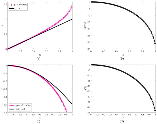
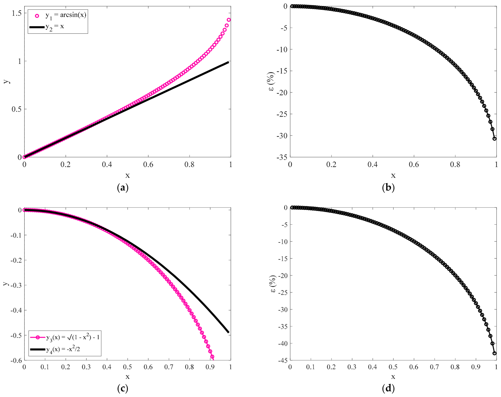
In Figure 1a, the $y_1\left(x\right)=\arcsin \left(x\right)$ and $y_2\left(x\right)=x$ curves are shown for comparison. The percentage differences between $y_1\left(x\right)$ and $y_2\left(x\right),$ defined as $\epsilon \left(\%\right)=\left|y_1\left(x\right)-y_2\left(x\right)\right|/y_1\left(x\right)\times 100\%$, are also shown in Figure 1b. In addition, in Figure 1c, the $y_3\left(x\right)=\sqrt{1-x^2}-1$ and $y_4\left(x\right)=-x^2/2$ are also presented. The percentage differences between $y_3\left(x\right)$ and $y_4\left(x\right)$are also shown in Figure 1d. It is evident that the first term approximations in Maclaurin series expansions presented in Equations (11) and (13) are accurate for $x\le 0.4$. In other words, it should be $a\ge 2.5b=2.5R_c\cos \left(\theta \right).$ It should be noted that the transition depth between the spherical and pyramidal parts of the indenter occurs when $a=b$. In addition, by substituting Equations (11) and (13) into Equation (6), we conclude in:

$$h-{\displaystyle \frac{a}{\tan \left(\theta \right)}}{\rm N}\left({\displaystyle \frac{\pi }{2}}-x\right)-{\displaystyle \frac{a^2}{2R_c}}{x}^2=0$$

(14)

Figure 1. (a) Comparison of the $y_1\left(x\right)=\arcsin \left(x\right)$ and $y_2\left(x\right)=x$ curves and (b) the percentage differences between them. (c) The $y_3\left(x\right)=\sqrt{1-x^2}-1$ and $y_4\left(x\right)=-x^2/2$ curves and (d) the percentage differences between them.

By combining Equations (7) and (14) we conclude in:

$$h-{\displaystyle \frac{a}{\tan \left(\theta \right)}}{\rm N}\left({\displaystyle \frac{\pi }{2}}-{\displaystyle \frac{b}{\alpha }}\right)-{\displaystyle \frac{b^2}{2R_c}}=0$$

(15)

By solving Equation (15) with respect to contact radius $a$, we conclude in:

$$a={\displaystyle \frac{2}{\pi N}}\tan \left(\theta \right)h+{\displaystyle \frac{2b}{\pi }}-{\displaystyle \frac{b^2\tan \left(\theta \right)}{\pi N{R}_c}}$$

(16)

In addition, by substituting Equation (4) into Equation (16):

$$a={\displaystyle \frac{2}{\pi N}}\tan \left(\theta \right)h+{\displaystyle \frac{2R_c\cos \left(\theta \right)}{\pi }}\left(1-{\displaystyle \frac{\sin \left(\theta \right)}{2N}}\right)$$

(17)

The contact radius as shown in Equation (17) will be calculated in the Pharr et al. generic differential equation [29]:

$${\displaystyle \frac{dF}{dh}}=2{\displaystyle \frac{{\rm E}}{1-v^2}}a\left(h\right)$$

(18)

where $E, v$ are the Young’s modulus and Poisson’s ratio of the tested material, respectively. It is important to note at this point that Equation (18) is valid for axisymmetric indenters with rotational symmetry, leading to a circular contact area between the indenter and the sample. Therefore, to proceed when considering a symmetric $n$-sided blunted-pyramidal tip, an indenter with rotational symmetry is assumed, leading to the same projected contact area (i.e., the one described by Equation (17)). By solving Equation (18) with respect to the applied force:

$$F=2{\displaystyle \frac{{\rm E}}{1-v^2}}{\displaystyle \underset{0}{\overset{h}{{\displaystyle \int }}}}a\left(u\right)du$$

(19)

where $u$ is the dummy integration parameter. Finally, by substituting Equation (17) into Equation (19), and considering that $F=0$at $h=0$ we conclude in:

$$F={\displaystyle \frac{2{\rm E}}{\left(1-v^2\right)\pi }}\left[{\displaystyle \frac{\tan \left(\theta \right)}{N}}{h}^2+2R_c\cos \left(\theta \right)\left(1-{\displaystyle \frac{\sin \left(\theta \right)}{2N}}\right)h\right]$$

(20)

In the limit $R_c\to 0$, Equation (20) is identical to Equation (1) for a 4-sided pyramidal indenter, as expected.

2.2. Simulated Curves

Open-access simulated datasets were employed, representing an elastic half-space with a Young’s modulus of $E=20 \mathrm{kPa}$ and a Poisson’s ratio of $v=0.5$. The datasets, generated using Mathematica 8.0, were designed to replicate realistic AFM force curves and included simulations for blunted 4-sided pyramidal indenters attached to a cantilever with a spring constant of 0.1 N/m. Tip radii of 100 nm and 200 nm were used, respectively, for a blunt pyramidal indenter with a semi-included angle of $\theta ={35}^{°}$. Randomly distributed Gaussian noise was added to the synthetic force-indentation data to mimic experimental variability. All datasets used in this study are publicly available in the AtomicJ repository (https://sourceforge.net/projects/jrobust/files/TestFiles, accessed on 1 July 2025 [30]).

2.3. Open-Access Experimental Data from the AtomicJ Repository

Human prostate carcinoma DU-145 cells were cultured in DMEM-F12 HAM medium (Sigma, St. Louis, MO, USA) supplemented with 10% fetal bovine serum and antibiotics and maintained at 37 °C in a humidified atmosphere containing 5% CO₂. Force-indentation measurements were performed using an Agilent 5500 Atomic Force Microscope (Agilent Technologies, Santa Clara, CA, USA) equipped with silicon nitride cantilevers (Veeco Probes, Plainview, NY, USA) featuring four-sided pyramidal tips with a nominal tip radius of 20 nm, a maximum manufacturer-reported tip radius of 60 nm, a half-angle of 25°, and a nominal spring constant of 0.01 N/m. The cantilever spring constant used for Young’s modulus determination was calibrated using the thermal tune method. All measurements were conducted in culture medium at 37 °C. The force-indentation data have been deposited in the AtomicJ repository (https://sourceforge.net/projects/jrobust/files/TestFiles/, accessed on 16 August 2025 [30]).

3. Results

3.1. Examining the Accuracy of Equation (20)

It is important to assess the accuracy of Equation (20) in comparison with the exact Equations (2) and (3). First, using Equation (17), we can evaluate the range of validity of the proposed approximation. As already mentioned, it should be:

$$\begin{gathered} a\ge 2.5R_c\cos \left(\theta \right)\Rightarrow {\displaystyle \frac{2}{\pi N}}\tan \left(\theta \right)h+{\displaystyle \frac{2R_c\cos \left(\theta \right)}{\pi }}\left(1-{\displaystyle \frac{\sin \left(\theta \right)}{N}}\right)\ge 2.5R_c\cos \left(\theta \right)\Rightarrow \\ h\ge {\displaystyle \frac{\pi {\rm N}{R}_c{\cos }^2\left(\theta \right)}{2\sin \left(\theta \right)}}\left[2.5-{\displaystyle \frac{2}{\pi }}\left(1-{\displaystyle \frac{\sin \left(\theta \right)}{N}}\right)\right] \end{gathered}$$

(21)

Therefore, the minimum ratio $h/R_c$ to use Equation (20) for data processing should be:

$${\displaystyle \frac{h_{min}}{R_c}}={\displaystyle \frac{\pi {\rm N}{\cos }^2\left(\theta \right)}{2\sin \left(\theta \right)}}\left[2.5-{\displaystyle \frac{2}{\pi }}\left(1-{\displaystyle \frac{\sin \left(\theta \right)}{N}}\right)\right]$$

(22)

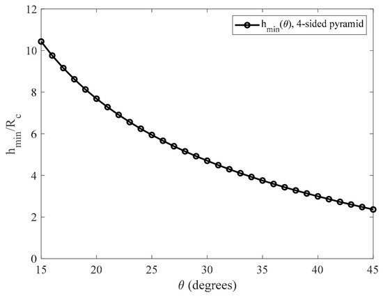
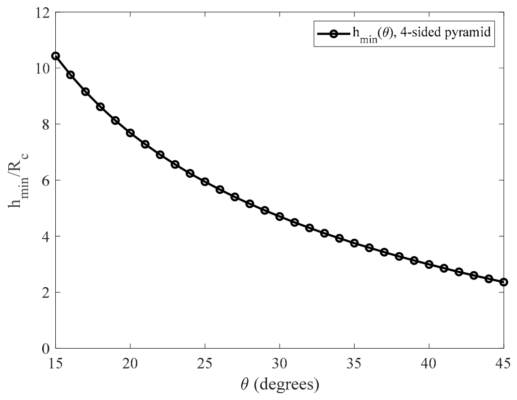
The ${\displaystyle \frac{h_{min}}{R_c}}$ ratios for different values of the angle $\theta$ are presented in Figure 2 and in Table 1 for the case of a 4-sided symmetric blunt pyramid.

Figure 2. The ${\displaystyle \frac{h_{min}}{R_c}}=f\left(\theta \right)$ curve in the domain ${15}^{°}\le \theta \le {45}^{°}$ for the case of a 4-sided symmetric blunt pyramidal indenter. For example, if $\theta ={35}^{°}$, the minimum indentation depth should be only ~3.8 times $R_c$ to use Equation (20).

Table 1. Characteristic $h_{min}/R_c$ values for different pyramids’ semi-included angles for the case of a 4-sided symmetric blunt pyramid.

θ (Degrees)	${\mathit{h}}_{\mathit{m}\mathit{i}\mathit{n}}/{\mathit{R}}_{\mathit{c}}$
15	10.4
20	7.7
25	5.9
30	4.7
35	3.8
40	3.0
45	2.4

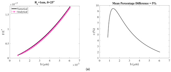
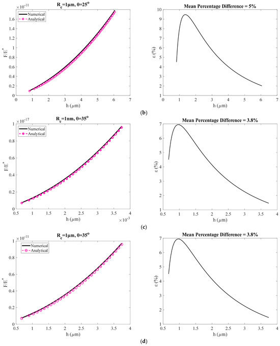
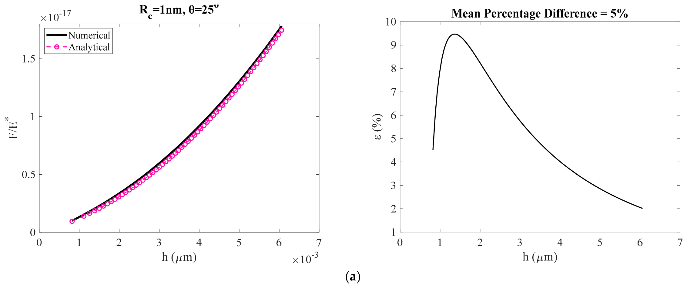
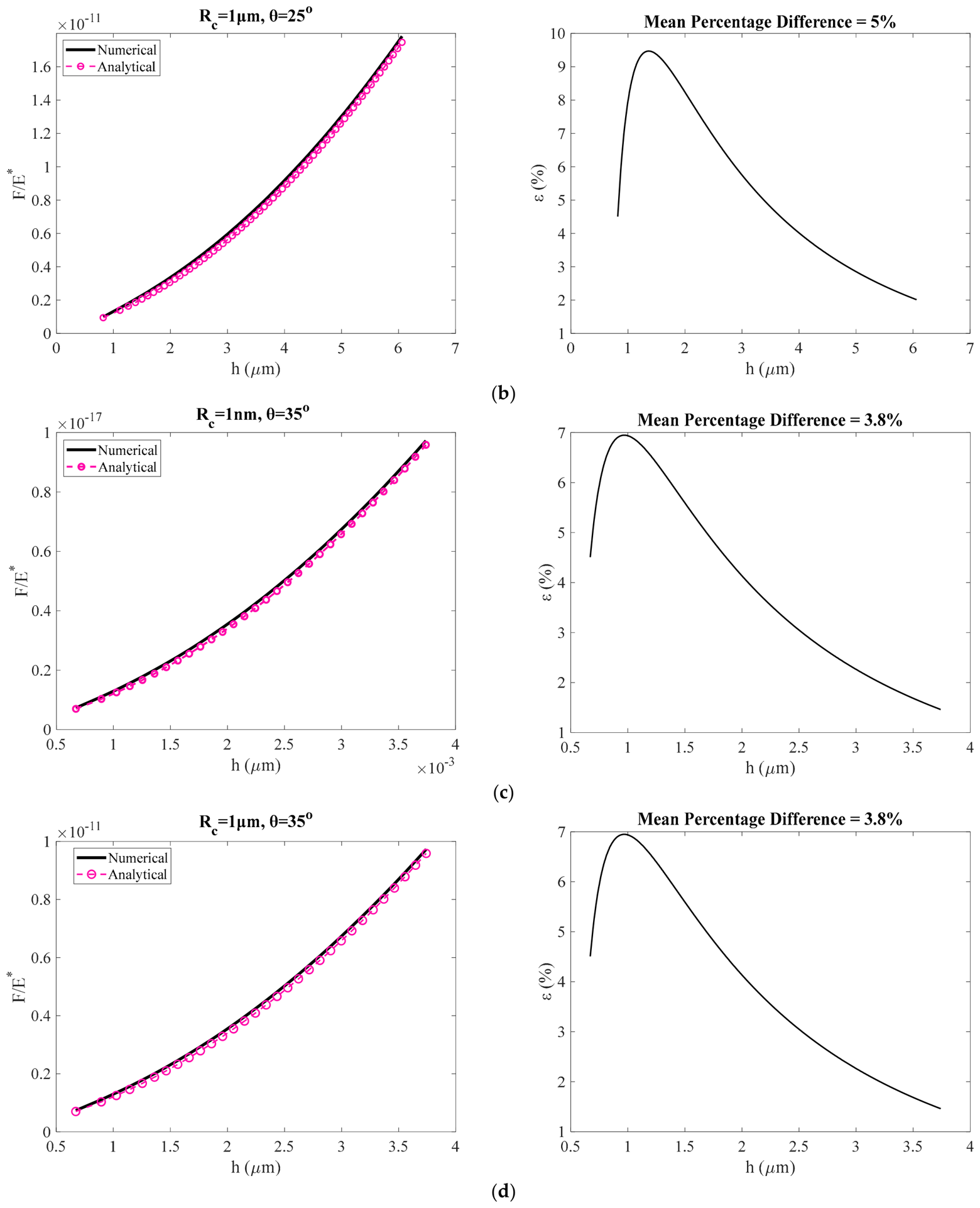
In Figure 3, we compare the results obtained using the classical equations (Equations (2)–(4)) with those obtained using the equation proposed in this paper (Equation (20)) for the case of a 4-sided symmetric blunt pyramid. In all cases, the $F/E^{*}=f\left(h\right)$ data, where $E^{*}=E/\left(1-v^2\right)$ is the reduced modulus, in the domain $b\le a\le 2.5b$ were plotted. Firstly, we calculated the indentation depth using Equation (3) for different values of $a$ in the domain above and also using $R_c=1 \mathrm{nm}$, $\theta ={25}^{°}$ (Figure 3a), $R_c=1 \mu \mathrm{m}$, $\theta ={25}^{°}$ (Figure 3b), $R_c=1 \mathrm{nm}$, $\theta ={35}^{°}$ (Figure 3c) and $R_c=1 \mu \mathrm{m}$, $\theta ={35}^{°}$ (Figure 3d). Subsequently, the $F/E^{*}$ ratio was calculated using Equation (2). The condition $a_{max}=2.5b$ results in different maximum indentation depths, as is evident from Figure 3, depending on the values of $R_c$ and $\theta$. In each case the percentage differences between the $F/E^{*}$ data when using Equations (2)–(4) and when using Equation (20) are shown.

Figure 3. (a) The $F/E^{*}=f\left(h\right)$ data and the resulting errors when using Equation (20), for the case of a 4-sided symmetric blunt pyramid, instead of the classic Equations (2)–(4) for:$R_c=1 \mathrm{nm}$, $\theta ={25}^{°}$ (a), $R_c=1 \mu \mathrm{m}$, $\theta ={25}^{°}$ (b), $R_c=1 \mathrm{nm}$, $\theta ={35}^{°}$ (c) and $R_c=1 \mu \mathrm{m}$, $\theta ={35}^{°}$ (d). The recorded errors are not influenced by the $R_c$ values for a given value of θ. On the contrary, indenters with small θ—values for a given value of $R_c$ lead to larger errors. The mean percentage differences between the exact and the approximate values are also presented in each case.

The error reduces as the indentation depth increases as expected. The recorded errors are not influenced by the $R_c$ values for a given value of $\theta$. On the contrary, indenters with small $\theta -$values for a given value of $R_c$ lead to larger errors. This is also evident by Figure 2 and Table 1, in which the $h_{min}/R_c$ ratio (i.e., minimum indentation depth with respect to $R_c$ in order to use the proposed Equation (20)) should be larger for small $\theta$. This is an interesting result. Why does the error for small indentation depths depend only on $\theta$? To understand this result, we need to correlate Equation (17) derived in this paper with the actual result (Equation (3)) at $a_0=b=R_c\cos \left(\theta \right)$. In this case, Equation (3) results in:

$$h_0=R_c{\cos }^2\left(\theta \right)$$

(23)

Using this result (i.e., Equation (23)), Equation (17) can also be written as follows:

$$\begin{gathered} a={\displaystyle \frac{2}{\pi N}}\tan \left(\theta \right)h_0+{\displaystyle \frac{2R_c\cos \left(\theta \right)}{\pi }}\left(1-{\displaystyle \frac{\sin \left(\theta \right)}{2N}}\right)\Rightarrow \\ a={\displaystyle \frac{2}{\pi N}}{\displaystyle \frac{\sin \left(\theta \right)}{\cos \left(\theta \right)}}{R}_c{\cos }^2\left(\theta \right)+{\displaystyle \frac{2R_c\cos \left(\theta \right)}{\pi }}\left(1-{\displaystyle \frac{\sin \left(\theta \right)}{2N}}\right)\Rightarrow \\ a={\displaystyle \frac{R_c\cos \left(\theta \right)}{\pi }}\left[{\displaystyle \frac{2}{N}}\sin \left(\theta \right)+2\left(1-{\displaystyle \frac{\sin \left(\theta \right)}{2N}}\right)\right]\Rightarrow \\ a={\displaystyle \frac{R_c\cos \left(\theta \right)}{\pi }}\left({\displaystyle \frac{\sin \left(\theta \right)}{N}}+2\right)\Rightarrow {\displaystyle \frac{a}{a_0}}={\displaystyle \frac{1}{\pi }}\left({\displaystyle \frac{\sin \left(\theta \right)}{N}}+2\right) \end{gathered}$$

(24)

In Equation (24), $a_0$ corresponds to the actual contact radius ($a_0=b=R_c\cos \left(\theta \right)$) and $a$ to the contact radius calculated using Equation (17). For large values of the parameter ${\displaystyle \frac{\sin \left(\theta \right)}{N}}$ (and as a result of the semi included angle θ for a given number of pyramid sides $n$) the ratio $a/a_0$ is close to unity. This is the reason for smaller errors when θ takes large values. In addition, the $a/a_0$ ratio does not depend on the $R_c$. Thus, different values of $R_c$ do not influence the calculated errors when the proposed approach is used.

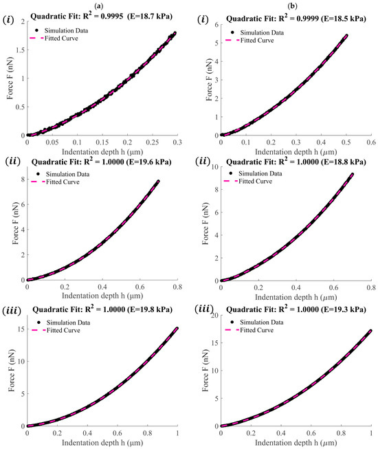
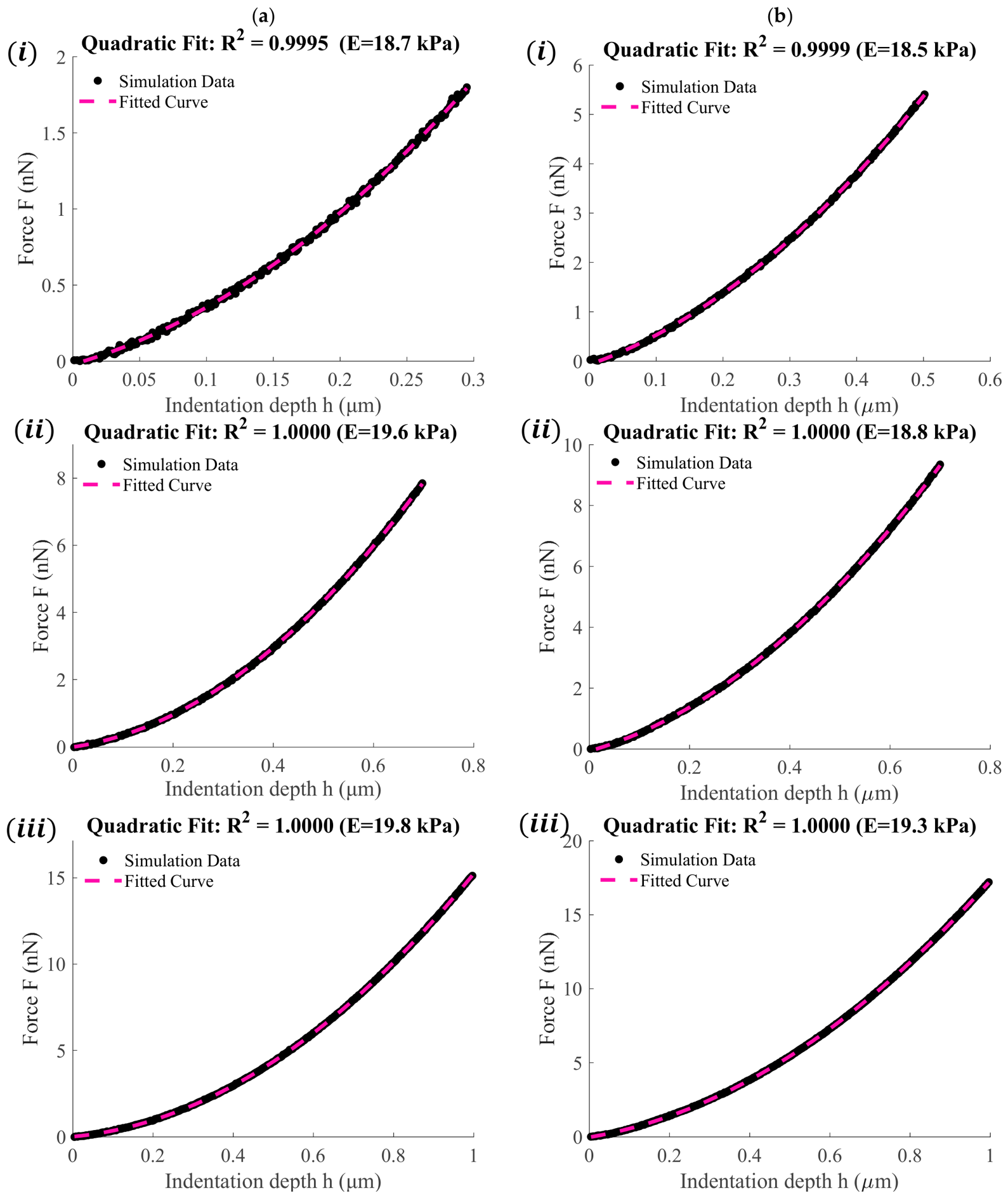
However, in all cases the $F/E^{*}$ values converge to the exact ones as the indentation depth increases. To further test the accuracy of the proposed Equation (Equation (20)), we used simulated data obtained by considering blunt 4-sided pyramidal indenters as described in Section 2.2. In all cases, the Young’s modulus was considered $E=20 \mathrm{kPa}$ and the Poisson’s ratio $v=0.5$. The goal is to fit the data to Equation (20) and test whether the Young’s modulus can be accurately determined. We present six characteristic curves. Figure 4a(i–iii) were obtained by considering $R_c=0.1 \mu \mathrm{m}$ and $h_{\max \left(1\right)}=300 \mathrm{nm}$, $h_{\max \left(2\right)}=700 \mathrm{nm}$ and $h_{\max \left(3\right)}=1000 \mathrm{nm}$. In addition, Figure 4b(i–iii) were obtained by considering $R_c=0.2 \mu \mathrm{m}$ and $h_{\max \left(1\right)}=500 \mathrm{nm}$, $h_{\max \left(2\right)}=700 \mathrm{nm}$ and $h_{\max \left(3\right)}=1000 \mathrm{nm}$. The Young’s moduli when using $R_c=0.1 \mu \mathrm{m}$ resulted in 18.7 kPa (Figure 4a(i)), 19.6 kPa (Figure 4a(ii)) and 19.8 kPa (Figure 4a(iii)). Furthermore, when using $R_c=0.2 \mu \mathrm{m}$, they resulted in 18.5 kPa (Figure 4b(i)), 18.8 kPa (Figure 4b(ii)) and 19.3 kPa (Figure 4b(iii)). As is evident by the results presented in Figure 4 for large indentation depths, the Young’s modulus calculated by the fitting process is nearly identical to the actual value of 20 kPa. It is also important to clarify that, in every case, the Young’s modulus was calculated solely from the quadratic coefficient obtained from the fitting procedure. The R-squared coefficient, used to evaluate the fitting process, is also presented in each case.

Figure 4. (a) Simulated force indentation data and fitted curves to Equation (20) when $R_c=0.1 \mu \mathrm{m}.$ (i) $h_{\max \left(1\right)}=300 \mathrm{nm}$, $E_1=18.7 \mathrm{kPa}$, (ii) $h_{\max \left(2\right)}=700 \mathrm{nm}$, $E_2=19.6 \mathrm{kPa}$ and (iii) $h_{\max \left(3\right)}=1000 \mathrm{nm}$, $E_3=19.8 \mathrm{kPa}$. (b) Simulated force indentation data and fitted curves to Equation (20) when $R_c=0.2 \mu \mathrm{m}.$ (i) $h_{\max \left(1\right)}=500 \mathrm{nm}$, $E_1=18.5 \mathrm{kPa}$, (ii) $h_{\max \left(2\right)}=700 \mathrm{nm}$, $E_2=18.8 \mathrm{kPa}$ and (iii) $h_{\max \left(3\right)}=1000 \mathrm{nm}$, $E_3=19.3 \mathrm{kPa}$.

3.2. Separation of Tip-Radius Effects from the Modulus-Dependent Quadratic Coefficient

Although Equation (20) contains two fitting coefficients, only the quadratic coefficient is employed for the calculation of the Young’s modulus. Crucially, as shown by its analytical definition, the quadratic coefficient governing the elastic response does not explicitly contain the tip-apex radius ($R_c$). While it is physically true that the raw experimental force-indentation data points are collectively influenced by the tip radius, the ordinary least-squares formulation separates the contributions associated with the two independent basis functions $h^2$ and h. Although these basis functions are not generally orthogonal, the solution of the normal equations uniquely identifies both coefficients simultaneously. Within the proposed analytical approximation, the effect of the blunt apex radius appears exclusively through the coefficient of the linear term. Consequently, Young’s modulus can be determined from the quadratic coefficient without requiring prior knowledge of the tip radius. This structural decoupling can be established rigorously by examining the Ordinary Least Squares (OLS) fitting procedure associated with the proposed force–indentation model.

The simplified force–indentation relationship derived in Equation (20) can be written as

$$F_i=C_1{h}_i^2+C_2{h}_i+{\epsilon }_i,$$

(25)

where $F_i$ and $h_i$denote the measured force and indentation depth corresponding to the $i$-th experimental point ($i=1,\dots ,m$), ${\epsilon }_i$ represents the residual error, and the coefficients $C_1$ and $C_2$ are defined as

$$C_1={\displaystyle \frac{2E}{\left(1-{\nu }^2\right)\pi }}{\displaystyle \frac{\tan \theta }{N}},$$

(26)

and

$$C_2={\displaystyle \frac{4E{R}_c\cos \theta }{\left(1-{\nu }^2\right)\pi }}\left(1-{\displaystyle \frac{\sin \theta }{2N}}\right).$$

(27)

The least-squares solution is obtained by minimizing the sum of squared residuals

$$S\left(C_1,C_2\right)={\displaystyle {\displaystyle \sum }_{i=1}^m}{\left(F_i-C_1{h}_i^2-C_2{h}_i\right)}^2.$$

(28)

The stationary point of Equation (28) is obtained by setting the partial derivatives with respect to both unknown coefficients equal to zero

$${\displaystyle \frac{\partial S}{\partial C_1}}=-2{\displaystyle {\displaystyle \sum }_{i=1}^m}{h}_i^2\left(F_i-{\widehat{C}}_1{h}_i^2-{\widehat{C}}_2{h}_i\right)=0,$$

(29)

$${\displaystyle \frac{\partial S}{\partial C_2}}=-2{\displaystyle {\displaystyle \sum }_{i=1}^m}{h}_i\left(F_i-{\widehat{C}}_1{h}_i^2-{\widehat{C}}_2{h}_i\right)=0.$$

(30)

Expanding Equations (29) and (30) yields the classical system of normal equations

$${\widehat{C}}_1{\displaystyle {\displaystyle \sum }_{i=1}^m}{h}_i^4+{\widehat{C}}_2{\displaystyle {\displaystyle \sum }_{i=1}^m}{h}_i^3={\displaystyle {\displaystyle \sum }_{i=1}^m}{F}_i{h}_i^2,$$

(31)

$${\widehat{C}}_1{\displaystyle {\displaystyle \sum }_{i=1}^m}{h}_i^3+{\widehat{C}}_2{\displaystyle {\displaystyle \sum }_{i=1}^m}{h}_i^2={\displaystyle {\displaystyle \sum }_{i=1}^m}{F}_i{h}_i.$$

(32)

These equations may be written in matrix form as:

$$\left[\begin{array}{cc}{\displaystyle {\displaystyle \sum }_{i=1}^m}{h}_i^4& {\displaystyle {\displaystyle \sum }_{i=1}^m}{h}_i^3\\ {\displaystyle {\displaystyle \sum }_{i=1}^m}{h}_i^3& {\displaystyle {\displaystyle \sum }_{i=1}^m}{h}_i^2\end{array}\right]\left[\begin{array}{c}{\widehat{C}}_1\\ {\widehat{C}}_2\end{array}\right]=\left[\begin{array}{c}{\displaystyle {\displaystyle \sum }_{i=1}^m}{F}_i{h}_i^2\\ {\displaystyle {\displaystyle \sum }_{i=1}^m}{F}_i{h}_i\end{array}\right].$$

(33)

The determinant of the coefficient matrix is

$$\Delta =\left({\displaystyle {\displaystyle \sum }_{i=1}^m}{h}_i^4\right)\left({\displaystyle {\displaystyle \sum }_{i=1}^m}{h}_i^2\right)-{\left({\displaystyle {\displaystyle \sum }_{i=1}^m}{h}_i^3\right)}^2$$

(34)

Since the basis functions $h^2$ and h are linearly independent over any non-trivial indentation interval (h > 0), the Cauchy–Schwarz inequality guarantees that:

$$\Delta >0,$$

(35)

ensuring the existence of a unique least-squares solution. Applying Cramer’s rule, the quadratic coefficient is obtained explicitly as:

$${\widehat{C}}_1={\displaystyle \frac{\left({{\displaystyle \sum }}_{i=1}^m{F}_i{h}_i^2\right)\left({{\displaystyle \sum }}_{i=1}^m{h}_i^2\right)-\left({{\displaystyle \sum }}_{i=1}^m{F}_i{h}_i\right)\left({{\displaystyle \sum }}_{i=1}^m{h}_i^3\right)}{\left({{\displaystyle \sum }}_{i=1}^m{h}_i^4\right)\left({{\displaystyle \sum }}_{i=1}^m{h}_i^2\right)-{\left({{\displaystyle \sum }}_{i=1}^m{h}_i^3\right)}^2}}.$$

(36)

Equation (36) demonstrates that the quadratic coefficient is uniquely determined from the experimental force–indentation measurements through the least-squares solution. Once ${\widehat{C}}_1$has been obtained, the Young’s modulus follows directly from Equation (26). Rearranging Equation (26) gives

$$E={\widehat{C}}_1 {\displaystyle \frac{\left(1-{\nu }^2\right)\pi N}{2\tan \theta }}$$

(37)

which provides the desired analytical expression for the elastic modulus. Substitution of the analytical force relationship $F_i=C_1{h}_i^2+C_2{h}_i$ into Equation (36) explicitly demonstrates that the least-squares estimate of the quadratic coefficient is unaffected by the linear coefficient $C_2$, since all terms containing $C_2$, and therefore $R_c$, cancel identically, yielding ${\widehat{C}}_1=C_1$:

$${\widehat{C}}_1={\displaystyle \frac{\left(C_1{{\displaystyle \sum }}_{i=1}^m{h}_i^4+C_2{{\displaystyle \sum }}_{i=1}^m{h}_i^3\right){{\displaystyle \sum }}_{i=1}^m{h}_i^2-\left(C_1{{\displaystyle \sum }}_{i=1}^m{h}_i^3+C_2{{\displaystyle \sum }}_{i=1}^m{h}_i^2\right){{\displaystyle \sum }}_{i=1}^m{h}_i^3}{\left({{\displaystyle \sum }}_{i=1}^m{h}_i^4\right)\left({{\displaystyle \sum }}_{i=1}^m{h}_i^2\right)-{\left({{\displaystyle \sum }}_{i=1}^m{h}_i^3\right)}^2}}$$

(38)

Expanding the numerator yields:

$${\widehat{C}}_1={\displaystyle \frac{C_1\left[\left({{\displaystyle \sum }}_{i=1}^m{h}_i^4\right)\left({{\displaystyle \sum }}_{i=1}^m{h}_i^2\right)-{({{\displaystyle \sum }}_{i=1}^m{h}_i^3)}^2\right]+C_2\left[\left({{\displaystyle \sum }}_{i=1}^m{h}_i^3\right)\left({{\displaystyle \sum }}_{i=1}^m{h}_i^2\right)-\left({{\displaystyle \sum }}_{i=1}^m{h}_i^2\right)\left({{\displaystyle \sum }}_{i=1}^m{h}_i^3\right)\right]}{\left({{\displaystyle \sum }}_{i=1}^m{h}_i^4\right)\left({{\displaystyle \sum }}_{i=1}^m{h}_i^2\right)-{\left({{\displaystyle \sum }}_{i=1}^m{h}_i^3\right)}^2}}$$

(39)

Since the terms containing $C_2$ cancel identically, the expression reduces to:

$${\widehat{C}}_1={\displaystyle \frac{C_1\left[\left({{\displaystyle \sum }}_{i=1}^m{h}_i^4\right)\left({{\displaystyle \sum }}_{i=1}^m{h}_i^2\right)-{({{\displaystyle \sum }}_{i=1}^m{h}_i^3)}^2\right]}{\left({{\displaystyle \sum }}_{i=1}^m{h}_i^4\right)\left({{\displaystyle \sum }}_{i=1}^m{h}_i^2\right)-{\left({{\displaystyle \sum }}_{i=1}^m{h}_i^3\right)}^2}}=C_1$$

(40)

Therefore, the least-squares estimate of the quadratic coefficient reduces exactly to ${\widehat{C}}_1=C_1$, irrespective of the value of $C_2$. This exact cancelation confirms that, within the proposed analytical framework, the Young’s modulus can be recovered directly from the quadratic coefficient. Once ${\widehat{C}}_1$ has been obtained, the Young’s modulus follows immediately from Equation (26). Since the tip radius $R_c$ appears only in the definition of the linear coefficient $C_2$and does not enter Equation (37), variations in the blunt-tip geometry do not affect the modulus calculation. Consequently, Young’s modulus can be determined without prior knowledge or calibration of the tip radius.

3.3. AFM Experiments on Prostate Cancer Cells

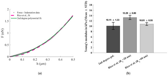
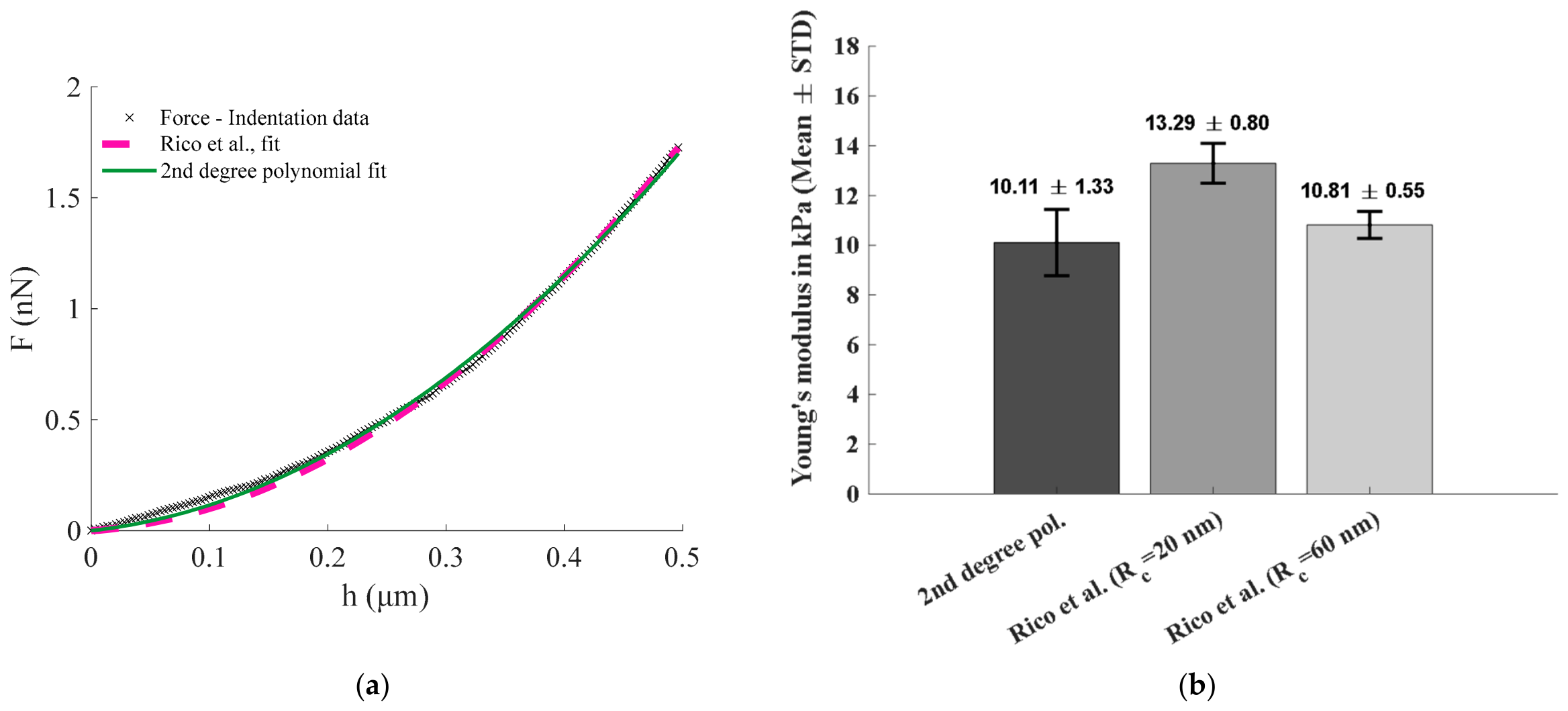
To further evaluate the practical applicability of the proposed formulation, experimental AFM nanoindentation data obtained from prostate cancer cells were analyzed. The force-indentation curves were obtained from the open-access AtomicJ repository and consisted of 10 individual measurements acquired using a four-sided pyramidal AFM probe. The data were first fitted using the exact equations of Rico et al. (Equations (2)–(5)) as implemented in the AtomicJ software. Since the original dataset did not provide the experimentally measured tip-apex radius, two representative values were considered: the nominal manufacturer value ($R_c=20 \mathrm{nm}$) and an upper-bound value ($R_c=60 \mathrm{nm}$) corresponding to the maximum tip radius specified by the manufacturer. The same force-indentation curves were subsequently fitted using the second-degree polynomial form of Equation (20), and the Young’s modulus was calculated directly from the quadratic fitting coefficient.

Figure 5a shows a representative force-indentation curve together with the fitting results obtained using the exact Rico et al. formulation and the proposed analytical approximation. In both cases, good agreement with the experimental measurements was observed. The corresponding Young’s modulus values are presented in Figure 5b and Table 2. The proposed method yielded a mean Young’s modulus of 10.11 ± 1.33 kPa, while application of the Rico et al. model resulted in values of 13.29 ± 0.80 kPa and 10.81 ± 0.55 kPa for $R_c=20 \mathrm{nm}$ and $R_c=60 \mathrm{nm}$, respectively.

Figure 5. (a) Force-indentation data obtained from a cancer cell using a four-sided pyramidal AFM tip. The data were fitted using the equations of Rico et al. (Equations (2)–(5)) implemented in the AtomicJ software and Equation (20) proposed in this paper. (b) Young’s modulus values calculated from 10 force-indentation curves using the coefficient of the quadratic term of Equation (20) and the equations of Rico et al., assuming $R_c=20$nm and $R_c=60$nm. For all fitting procedures, the R-squared coefficient was greater than 0.98. The mean ± standard deviation for each case is presented in the graph.

Table 2. Young’s modulus values obtained from 10 force-indentation curves using the quadratic coefficient of Equation (20) and the equations of Rico et al. (Equations (2)–(5)), assuming a tip radius of 20 nm and 60 nm.

2nd Degree pol. fit. (kPa)	Rico et al. (Rc = 20 nm) (kPa)	Rico et al. (Rc = 60 nm) (kPa)
13.00	14.30	11.37
11.60	14.10	11.36
10.70	13.90	11.23
10.34	13.26	10.79
9.58	13.19	10.77
9.55	13.24	10.80
9.09	12.74	10.45
8.86	11.92	9.86
9.32	14.00	11.40
9.01	12.28	10.11

These results are particularly noteworthy because a change in the assumed tip radius from 20 nm to 60 nm produced a large variation in the Young’s modulus calculated using the Rico et al. formulation. In contrast, the proposed approach produced a unique modulus estimate without requiring any prior knowledge of the tip geometry. The modulus obtained using Equation (20) was also in very good agreement with the value obtained from the exact Rico et al. equations when the larger tip radius was assumed. Therefore, the experimental analysis supports the central conclusion of this work that reliable modulus estimation can be achieved without explicit knowledge of the tip-apex radius, which is often unavailable in routine AFM experiments.

4. Discussion

The approximate force–indentation relation introduced in this work (Equation (20)) offers a straightforward analytical expression suitable for processing data obtained with $n$-sided blunt pyramidal indenters. Comparison with the exact formulations of Rico et al. [27] showed that the proposed expression preserves high accuracy across a broad range of indentation depths. The evaluation of the percentage differences indicated that the discrepancy decreases with increasing indentation, as anticipated, since the first-order approximations employed in the derivation become progressively more accurate for larger contact areas. However, Equation (20) can also be used for small indentations; we provide a characteristic threshold of $a\ge 2.5b$, which results in Table 1. The condition $a\ge 2.5b$ is not an experimentally determined quantity but follows directly from the validity of the first-order Maclaurin expansions employed in Equations (11) and (13). Specifically, Figure 1 shows that when $x=b/a\le 0.4$, the percentage errors associated with the approximations remain relatively small. For this reason, the criterion $a\ge 2.5b$ was adopted as a practical lower bound for the application of the proposed model. Since this requirement originates solely from geometric considerations, it depends only on the indenter geometry and not on the elastic properties of the tested material. Thus, the central finding of this study is that the validity of the proposed analytical approximation is governed primarily by indentation depth. This has direct practical implications for AFM nanoindentation. The geometry-dependent criterion given by Equation (22) provides a simple means of identifying the minimum indentation depth required for reliable application of Equation (20). As demonstrated in Figure 3, the approximation rapidly converges toward the exact solution once this threshold is exceeded. Importantly, the threshold depends only on the indenter geometry, through the semi-included angle and number of pyramid sides, and is independent of the mechanical properties of the tested material.

A key outcome is that the accuracy of the approximation depends on the semi-included angle $\theta$ and the number of sides of the symmetric pyramid (through the dependence on the factor $N={\displaystyle \frac{n}{\pi }}\sin \left({\displaystyle \frac{\pi }{n}}\right)$), rather than on the tip radius $R_c$. This behavior was clarified by examining the ratio of the exact and approximate contact radii (Equation (24)). As shown analytically, the ratio is close to unity when the term $\sin \left(\theta \right)/{\rm N}$ increases, explaining the reduced error for indenters with larger semi-included angles. Conversely, sharper indenters (small $\sin \left(\theta \right)/{\rm N}$ ratios) require deeper indentations to satisfy the condition $a\ge 2.5b$. This dependency was captured and summarized in Table 1, which provides practical thresholds for experimental implementation.

The new equation was also tested on simulated data, as described in Section 2.2. This is an important procedure, since it examines whether the new equation can effectively capture the entire data range, from the spherical region to the pyramidal region of the indenter. The fitting results further confirmed that the approximation performs well under realistic conditions. Despite the presence of noise and tip–sample interaction complexity, the Young’s modulus extracted from Equation (20) closely matched the true value of 20 kPa in all tested cases.

Overall, the proposed approach offers several advantages. First, it eliminates the need to separately fit the spherical and pyramidal regimes, thereby simplifying the data-processing workflow. Second, it provides an analytical expression that does not require numerical integration, making it suitable for automated processing and large datasets. Third, the force–indentation data can be fitted directly using the second-degree polynomial form of Equation (20), while the Young’s modulus can be determined solely from the quadratic coefficient (Equation (37)). Consequently, the tip-apex radius is not required as an input parameter for the final modulus calculation, thereby reducing a potential source of uncertainty in AFM-based mechanical characterization. This feature is particularly relevant for biological samples, for which AFM probes may exhibit deviations from their nominal geometry because of manufacturing imperfections, tip wear, contamination, or interactions with the sample. Such effects can be especially important in liquid environments, where adsorption of biological material onto the probe may modify its effective geometry. Thus, the effective tip-apex radius may differ from the nominal manufacturer-specified value and may evolve during an experiment, introducing uncertainty into conventional indentation analyses that explicitly require the tip radius. By accounting analytically for apex rounding while retaining a simple polynomial fitting procedure, the present formulation provides a practical alternative for routine AFM indentation measurements, particularly when large datasets require rapid and reproducible quantitative analysis.

It is also important to note that Equation (20) also includes the case of blunted conical indenters. In particular, let us examine the term $N$ (Equation (8)). We can also use a Maclaurin series expansion for the term $\sin \left({\displaystyle \frac{\pi }{n}}\right):$

$$\sin \left({\displaystyle \frac{\pi }{n}}\right)={\displaystyle {\displaystyle \sum }_{k=0}^{\infty }}{\displaystyle \frac{{\left(-1\right)}^k{\left(\frac{\pi }{n}\right)}^{1+2k}}{\left(1+2k\right)!}}$$

(41)

For small $\pi /n$ ratios we keep only the first term in Equation (41), thus:

$$\sin \left({\displaystyle \frac{\pi }{n}}\right)\cong {\displaystyle \frac{\pi }{n}}$$

(42)

Equation (42) is valid when $n\gg \pi$. The case where $n\to \infty$ is the one describing a sphero-conical indenter. In this case, the term $N$ in Equation (8) tends to unity and Equation (20) can be written as below:

$$F={\displaystyle \frac{2{\rm E}}{\left(1-v^2\right)\pi }}\left[\tan \left(\theta \right)h^2+2R_c\cos \left(\theta \right)\left(1-{\displaystyle \frac{\sin \left(\theta \right)}{2}}\right)h\right]$$

(43)

A key assumption underlying the analysis presented in this paper is that the indenter can be treated as axisymmetric, thereby allowing the generic indentation equation given by Equation (18) to be applied. The use of equivalent axisymmetric geometries is well established in indentation mechanics. For instance, Oliver and Pharr approximated the Berkovich indenter, a three-sided pyramidal geometry that is inherently non-axisymmetric, by an equivalent conical indenter with the same depth-to-projected-area relationship [31]. This approach is based on the premise that the projected contact area is a dominant parameter governing the indentation response. The present work follows a similar approach.

From a mathematical perspective, the validity of this approximation improves as the number of sides of the pyramidal indenter increases. As demonstrated by Equations (41) and (42), in the limiting case $n\to \infty$, the pyramidal geometry converges to a cone, for which the axisymmetric representation becomes exact. Furthermore, the validity of the approximation can be assessed indirectly through the comparison with the exact Rico et al. solution (Equations (2)–(5)). As demonstrated in Figure 3, the discrepancy between the proposed Equation (20) and the exact solution decreases systematically with increasing indentation depth and becomes very small for the indentation range defined by Equation (22). Since Equation (20) contains both the axisymmetric-contact assumption and the first-order Maclaurin expansions introduced in Equations (11) and (13), the reported errors represent the combined effect of all approximations employed in the derivation. The convergence of Equation (20) to the exact Rico et al. solution therefore indicates that the axisymmetric representation does not introduce a dominant error within the intended range of application of the model.

A further question concerns the applicability of the proposed approach to heterogeneous biological materials. Biological tissues are often characterized by pronounced depth-dependent variations in their mechanical properties due to their structural heterogeneity [32,33,34]. Nevertheless, from a mathematical perspective, the methodology presented in this work remains applicable to heterogeneous samples. According to Equation (17), for indentation depths exceeding the transition depth ($h>h_T$), the contact radius can be written in the linear form

$$a\left(h\right)=Ah+B,$$

(44)

where $A$ and $B$ are constants that depend solely on the geometry of the indenter. Specifically,

$$A={\displaystyle \frac{2}{\pi N}}\tan \left(\theta \right)$$

(45)

and,

$$B={\displaystyle \frac{2R_c\cos \left(\theta \right)}{\pi }}\left(1-{\displaystyle \frac{\sin \left(\theta \right)}{2N}}\right)$$

(46)

For a heterogeneous material, the Young’s modulus becomes depth dependent, that is: $E=E\left(h\right).$In this case, the generic indentation equation (Equation (18)) can be written as

$${\displaystyle \frac{dF}{dh}}={\displaystyle \frac{2E\left(h\right)}{1-{\nu }^2}}a\left(h\right).$$

(47)

Substituting Equation (44) into Equation (47) and integrating over the indentation depth yields:

$$F={\displaystyle \frac{2}{1-{\nu }^2}}{{\displaystyle \int }}_0^{h}E\left(u\right)\left(Au+B\right) du.$$

(48)

where $u$ is the dummy integration variable. Equation (48) may be rewritten as:

$$F={\displaystyle \frac{2}{1-{\nu }^2}}{{\displaystyle \int }}_0^{h}f\left(u\right)g\left(u\right) du,$$

(49)

where $f\left(u\right)=E\left(u\right)$and $g\left(u\right)=Au+B.$Assuming that $E\left(u\right)$ is continuous within the indentation interval, the weighted mean value theorem for integrals [35] guarantees the existence of a point $c\in \left(0,h\right)$such that

$${{\displaystyle \int }}_0^{h}f\left(u\right)g\left(u\right) du=f\left(c\right){{\displaystyle \int }}_0^{h}g\left(u\right) du.$$

(50)

Therefore,

$$F={\displaystyle \frac{2E\left(c\right)}{1-{\nu }^2}}{{\displaystyle \int }}_0^h(\left.Au+B\right) du,$$

(51)

which leads to

$$F={\displaystyle \frac{AE\left(c\right)}{1-{\nu }^2}}{h}^2+{\displaystyle \frac{2BE\left(c\right)}{1-{\nu }^2}}h.$$

(52)

Equation (52) has exactly the same mathematical structure as Equation (20), with the constant Young’s modulus replaced by an effective (or ‘average’) modulus $E\left(c\right)$ corresponding to a characteristic depth within the interval $\left(0,h\right)$. Consequently, the proposed fitting procedure remains mathematically valid even for highly heterogeneous materials. In such cases, the extracted modulus should be interpreted as an effective depth-averaged modulus associated with the indentation interval.

In addition, it should be emphasized that the analysis presented in this paper assumes purely elastic material behavior and does not account for viscoelastic effects. Consequently, the proposed approach should be applied only under experimental conditions for which viscoelastic contributions are negligible. Such conditions can be approached by limiting the indentation rate, as demonstrated in previous AFM studies on biological materials [36,37,38,39,40,41]. Therefore, the proposed model should be regarded as a quasi-static approximation. Furthermore, a criterion establishing when the elastic approximation remains valid has been presented previously [41]. Therefore, the applicability of the present model depends not only on the indenter geometry and indentation depth but also on the selection of experimental conditions that minimize time-dependent mechanical effects.

It should also be noted that the principal contribution of the proposed approach is not to surpass the accuracy of the exact Rico et al. formulation (Equations (2)–(4)), which remains the most rigorous description of blunt pyramidal indentation. Instead, its value lies in providing a practical compromise between accuracy and computational simplicity. In routine AFM studies, the exact blunt-pyramid equations are often avoided because of their numerical complexity, and researchers commonly employ the considerably simpler Sneddon equation or its pyramidal counterpart, both of which neglect the rounded tip apex. The closed-form expression derived in this work retains the simplicity of a second-degree polynomial fitting procedure while accounting for tip blunting. Consequently, it offers improved mechanical characterization compared with ideal sharp-tip models without introducing the computational burden associated with the exact blunt-pyramid formulation. Furthermore, because Young’s modulus is determined solely from the quadratic coefficient of the fitted equation, explicit knowledge of the tip-apex radius is not required, eliminating an additional source of uncertainty during modulus estimation.

It is also important to note that the presented approach has several limitations. In particular, as already mentioned, it was derived for linear elastic materials, whereas soft biological samples often exhibit nonlinear elastic or viscoelastic behavior. However, since under specific experimental conditions (i.e., low indentation rates [41] and large indentation depths [34]) the linear elastic approximation is commonly used in the literature, the proposed new equation (Equation (20)) will serve as a powerful tool for researchers in the AFM indentation field. In addition, the derivation assumes an ideal symmetric blunt pyramidal geometry characterized by a constant semi-included angle and a rounded apex. Therefore, deviations from this geometry resulting from manufacturing imperfections, tip wear, contamination, or probe damage may introduce additional errors that are not accounted for by the model. In addition, as previously mentioned, Equation (20) becomes accurate for $a>2.5b$. For small indentation depths, where $a\approx b$, it introduces non-negligible errors. Consequently, the proposed approach is not recommended for force curves dominated by the very initial stages of contact, where the interaction is governed primarily by the spherical apex and higher-order geometric effects become significant.

A further limitation concerns material-indenter interactions. The model assumes frictionless and non-adhesive contact between the indenter and the sample. While this assumption is commonly adopted in AFM nanoindentation analysis, biological materials may exhibit adhesive interactions, surface forces, or structural heterogeneities that modify the measured response, particularly at shallow indentation depths. Therefore, the proposed equation should be regarded as most appropriate for conditions under which elastic deformation dominates the contact behavior.

Nevertheless, the assumption of adhesionless contact is generally consistent with common AFM practice for biological samples. AFM probes are frequently passivated using non-adhesive coatings, such as polyethylene glycol, while measurements are often performed in liquid environments that mimic physiological conditions and substantially reduce adhesion forces. Under such conditions, adhesion forces are typically one to two orders of magnitude smaller than those observed in air [23,42,43,44,45]. Although specific tip-sample interactions, including electrostatic or chemical bonding effects, may still occur, their contribution is generally small compared with the elastic forces considered in the present study. Furthermore, the indentation depths examined often exceed the range in which adhesion dominates the contact response, ensuring that elastic contributions remain the primary factor governing the measured force-indentation behavior. Consequently, the assumption of non-adhesive contact remains widely accepted in AFM studies of soft biological materials [45].

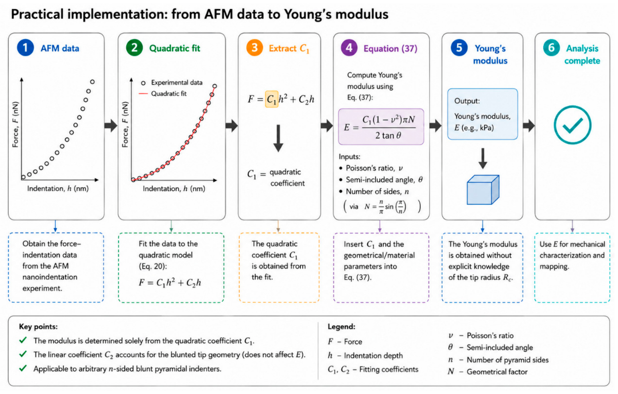
Table 3 summarizes the principal novel elements of the proposed approach compared with the current state of the art, highlighting their practical significance. In addition, Figure 6 provides an overview of the proposed workflow for determining the Young’s modulus of a soft sample using an n-sided blunt pyramidal indenter.

Table 3. Principal scientific contributions of the proposed analytical model compared with the existing state of the art.

Novel Element	Previous State of the Art	Contribution of This Work	Practical Significance
Closed-form analytical solution for blunt pyramidal indentation	Existing blunt-pyramid models (Rico et al. [27]) rely on coupled implicit equations and numerical evaluation.	Derivation of a closed-form force–indentation equation for an arbitrary n-sided blunt pyramidal indenter.	Eliminates iterative numerical calculations and significantly simplifies AFM data analysis.
General analytical framework for arbitrary indenter geometries	Most analytical models are limited to conical or four-sided pyramidal indenters and are treated independently.	Development of a unified formulation valid for arbitrary n-sided pyramidal indenters, naturally recovering the sphero-conical solution as n → ∞.	Extends the applicability of the model to a broad range of AFM probe geometries within a single theoretical framework.
Analytical characterization of the approximation	Simplified blunt-tip approximations rarely include rigorous validity limits or systematic error analysis.	Establishment of the validity criterion ($a$ ≥ 2.5 b), quantitative error analysis, and demonstration that the approximation accuracy is governed primarily by pyramid geometry rather than the tip apex radius.	Provides clear guidelines for selecting the appropriate indentation range and assessing the expected accuracy of the approximation.
Young’s modulus determination without explicit knowledge of the tip apex radius	Conventional blunt-tip analyses require the tip apex radius as an explicit input parameter during modulus calculation.	Reformulation of the force–indentation relationship as a quadratic polynomial in which the Young’s modulus is obtained directly from the quadratic fitting coefficient, eliminating the need for explicit knowledge of the tip apex radius.	Removes the need for tip apex radius calibration during modulus extraction, thereby reducing one of the major sources of uncertainty in AFM nanoindentation analysis.

Figure 6. Workflow for determining Young’s modulus from AFM indentation data using the proposed analytical model.

The potential applications of the proposed approach are not limited strictly to mechanical characterization. Advanced functional AFM techniques, such as conductive-AFM (c-AFM), AFM-based electrophysiology [46], and Kelvin Probe Force Microscopy (KPFM) [47], are increasingly combined with force measurements to obtain simultaneous mechanical and functional data from biological samples. Since the geometry of the AFM tip apex directly affects both the contact area and the spatial localization of the measured signals, the analytical description of blunt pyramidal probes developed here can contribute to a more accurate interpretation of these multi-signal, multifunctional measurements.

5. Conclusions

This study presents a new approximate analytical force–indentation equation for AFM experiments using arbitrary n-sided blunt pyramidal indenters. By combining first-order geometric approximations with the general indentation differential equation, the proposed formulation provides a closed-form relationship between applied force and indentation depth, avoiding the numerical solution of coupled nonlinear equations required by existing exact formulations.

Comparison with the exact solutions of Rico et al. (Equations (2)–(5)) demonstrated that the approximation becomes increasingly accurate with increasing indentation depth, with the associated error primarily governed by the indenter geometry, particularly the semi-included angle $\theta$ and the number of pyramid sides $n$. A practical criterion for the minimum indentation depth required for reliable application of the model was established, while validation using simulated and experimental AFM datasets confirmed its ability to accurately recover the Young’s modulus over a broad range of realistic conditions. Importantly, within the proposed formulation, the Young’s modulus is determined directly from the quadratic coefficient of the fitted force–indentation curve, while the tip-apex radius contributes only to the linear term. This reduces the dependence of modulus determination on precise characterization of the blunt tip apex.

The formulation provides a unified analytical framework for blunt pyramidal indentation and naturally recovers the previously reported sphero-conical solution in the limit $n\to \infty .$ Although developed within the framework of linear elastic contact mechanics and subject to reduced accuracy at very small indentation depths, the proposed methodology provides a practical balance between computational efficiency and predictive accuracy. In addition, its mathematical framework can be extended to heterogeneous materials, yielding an effective Young’s modulus corresponding to a depth-averaged representation of the local mechanical properties. Its applicability to arbitrary blunt pyramidal geometries, reduced sensitivity to tip-radius uncertainty, and computational efficiency make it particularly suitable for automated AFM data analysis and the mechanical characterization of complex and heterogeneous biological materials.

References

- Amabili, M.; Asgari, M.; Breslavsky, I.D.; Franchini, G.; Giovanniello, F.; Holzapfel, G.A. Microstructural and mechanical characterization of the layers of human descending thoracic aortas. Acta Biomater. 2021, 134, 401–421. [Google Scholar] [CrossRef] [Scilit] [PubMed]
- Stylianou, A.; Kontomaris, S.V.; Grant, C.; Alexandratou, E. Atomic Force Microscopy on Biological Materials Related to Pathological Conditions. Scanning 2019, 2019, 8452851. [Google Scholar] [CrossRef] [Scilit] [PubMed]
- Joo, S.; Eom, S.; Choi, Y.; Jeong, U.; Cho, Y.; Yu, W.; Park, K.; Hong, S. Atomic Force Microscopy for Cross-Disciplinary Materials Research. Small Methods 2025, 9, 2500514. [Google Scholar] [CrossRef] [Scilit] [PubMed]
- Stylianou, A.; Lekka, M.; Stylianopoulos, T. AFM assessing of nanomechanical fingerprints for cancer early diagnosis and classification: From single cell to tissue level. Nanoscale 2018, 10, 20930–20945. [Google Scholar] [CrossRef] [Scilit] [PubMed]
- Lekka, M. Discrimination between Normal and Cancerous Cells Using AFM. BioNanoScience 2016, 6, 65–80. [Google Scholar] [CrossRef] [Scilit] [PubMed]
- Plodinec, M.; Loparic, M.; Monnier, C.A.; Obermann, E.C.; Zanetti-Dallenbach, R.; Oertle, P.; Hyotyla, J.T.; Aebi, U.; Bentires-Alj, M.; Lim, R.Y.H.; et al. The nanomechanical signature of breast cancer. Nat. Nanotechnol. 2012, 7, 757–765. [Google Scholar] [CrossRef] [Scilit] [PubMed]
- Najera, J.; Rosenberger, M.R.; Datta, M. Atomic Force Microscopy Methods to Measure Tumor Mechanical Properties. Cancers 2023, 15, 3285. [Google Scholar] [CrossRef] [Scilit] [PubMed]
- Stolz, M.; Gottardi, R.; Raiteri, R.; Miot, S.; Martin, I.; Imer, R.; Staufer, U.; Raducanu, A.; Dueggelin, M.; Baschong, W.; et al. Early detection of aging cartilage and osteoarthritis in mice and patient samples using atomic force microscopy. Nat. Nanotechnol. 2009, 4, 186–192. [Google Scholar] [CrossRef] [Scilit] [PubMed]
- Asgari, M.; Latifi, N.; Giovanniello, F.; Espinosa, H.D.; Amabili, M. Revealing Layer-Specific Ultrastructure and Nanomechanics of Fibrillar Collagen in Human Aorta via Atomic Force Microscopy Testing: Implications on Tissue Mechanics at Macroscopic Scale. Adv. NanoBiomed Res. 2022, 2, 2100159. [Google Scholar] [CrossRef] [Scilit]
- Andriotis, O.G.; Manuyakorn, W.; Zekonyte, J.; Katsamenis, O.L.; Fabri, S.; Howarth, P.H.; Davies, D.E.; Thurner, P.J. Nanomechanical assessment of human and murine collagen fibrils via atomic force microscopy cantilever-based nanoindentation. J. Mech. Behav. Biomed. Mater. 2014, 39, 9–26. [Google Scholar] [CrossRef] [Scilit] [PubMed]
- Ramalho, R.; Rankovic, S.; Zhou, J.; Aiken, C.; Rousso, I. Analysis of the mechanical properties of wild type and hyperstable mutants of the HIV-1 capsid. Retrovirology 2016, 13, 17. [Google Scholar] [CrossRef] [Scilit] [PubMed]
- Xia, F.; Youcef-Toumi, K. Review: Advanced Atomic Force Microscopy Modes for Biomedical Research. Biosensors 2022, 12, 1116. [Google Scholar] [CrossRef] [Scilit] [PubMed]
- Collinson, D.W.; Sheridan, R.J.; Palmeri, M.J.; Brinson, L.C. Best Practices and Recommendations for Accurate Nanomechanical Characterization of Heterogeneous Polymer Systems with Atomic Force Microscopy. Prog. Polym. Sci. 2021, 119, 101420. [Google Scholar] [CrossRef] [Scilit]
- Kim, E.; Ramos Figueroa, A.L.; Schrock, M.; Zhang, E.; Newcomb, C.J.; Bao, Z.; Michalek, L. A Guide for Nanomechanical Characterization of Soft Matter via AFM: From Mode Selection to Data Reporting. STAR Protoc. 2025, 6, 103809. [Google Scholar] [CrossRef] [Scilit] [PubMed]
- Kontomaris, S.-V.; Yova, D.; Stylianou, A.; Politopoulos, K. The Significance of the Percentage Differences of Young’s Modulus in the AFM Nanoindentation Procedure. Micro Nanosyst. 2015, 7, 86–97. [Google Scholar] [CrossRef] [Scilit]
- Kontomaris, S.V.; Stylianou, A.; Malamou, A.; Nikita, K.S. An Alternative Approach for the Young’s Modulus Determination of Biological Samples Regarding AFM Indentation Experiments. Mater. Res. Express 2019, 6, 025407. [Google Scholar] [CrossRef] [Scilit]
- Persano, F.; Parodi, A.; Pallaeva, T.; Kolesova, E.; Zamyatnin, A.A., Jr.; Pokrovsky, V.S.; De Matteis, V.; Leporatti, S.; Cascione, M. Atomic Force Microscopy: A Versatile Tool in Cancer Research. Cancers 2025, 17, 858. [Google Scholar] [CrossRef] [Scilit] [PubMed]
- Matias, Z.; Lopes, C.S.; Santos, N.C.; Carvalho, F.A. Nanotechnology Meets Medicine: Applications of Atomic Force Microscopy in Disease. Biophys. Rev. 2025, 17, 359–384. [Google Scholar] [CrossRef] [Scilit] [PubMed]
- Marcuello, C.; Lim, K.S.; Nisini, G.; Pokrovsky, V.S.; Conde, J.; Ruggeri, F.S. Nanoscale Analysis beyond Imaging by Atomic Force Microscopy: Molecular Perspectives on Oncology and Neurodegeneration. Small Sci. 2025, 5, e202500351. [Google Scholar] [CrossRef] [Scilit] [PubMed]
- Deng, X.; Xiong, F.; Li, X.; Xiang, B.; Li, Z.; Wu, X.; Guo, C.; Li, X.; Li, Y.; Li, G.; et al. Application of atomic force microscopy in cancer research. J. Nanobiotechnol. 2018, 16, 102. [Google Scholar] [CrossRef] [Scilit] [PubMed]
- Thomas-Chemin, O.; Janel, S.; Boumehdi, Z.; Séverac, C.; Trevisiol, E.; Dague, E.; Duprés, V. Advancing High-Throughput Cellular Atomic Force Microscopy with Automation and Artificial Intelligence. ACS Nano 2025, 19, 5045–5062. [Google Scholar] [CrossRef] [Scilit] [PubMed]
- Zemła, J.; Bobrowska, J.; Kubiak, A.; Zieliński, T.; Pabijan, J.; Pogoda, K.; Bobrowski, P.; Lekka, M. Indenting soft samples (hydrogels and cells) with cantilevers possessing various shapes of probing tip. Eur. Biophys. J. 2020, 49, 485–495. [Google Scholar] [CrossRef] [Scilit] [PubMed]
- Krieg, M.; Fläschner, G.; Alsteens, D.; Gaub, B.M.; Roos, W.H.; Wuite, G.J.; Gaub, H.E.; Gerber, C.; Dufrêne, Y.F.; Müller, D.J. Atomic force microscopy-based mechanobiology. Nat. Rev. Phys. 2019, 1, 41–57. [Google Scholar] [CrossRef] [Scilit]
- Yang, W.; Lacroix, D.; Tan, L.P.; Chen, J. Revealing the nanoindentation response of a single cell using a 3D structural finite element model. J. Mater. Res. 2021, 36, 2591–2600. [Google Scholar] [CrossRef] [Scilit]
- Owen, D.S. Toward a better modulus at shallow indentations—Enhanced tip and sample characterization for quantitative atomic force microscopy. Microsc. Res. Tech. 2023, 86, 84–96. [Google Scholar] [CrossRef] [Scilit] [PubMed]
- Offroy, M.; Razafitianamaharavo, A.; Beaussart, A.; Pagnout, C.; Duval, J.F.L. Fast automated processing of AFM PeakForce curves to evaluate spatially resolved Young modulus and stiffness of turgescent cells. RSC Adv. 2020, 10, 19258–19275. [Google Scholar] [CrossRef] [Scilit] [PubMed]
- Rico, F.; Roca-Cusachs, P.; Gavara, N.; Farré, R.; Rotger, M.; Navajas, D. Probing mechanical properties of living cells by atomic force microscopy with blunted pyramidal cantilever tips. Phys. Rev. E 2005, 72, 021914. [Google Scholar] [CrossRef] [Scilit] [PubMed]
- Kontomaris, S.V.; Malamou, A.; Stylianou, A. Development of an accurate simplified approach for data processing in AFM indentation experiments. Micron 2025, 190, 103782. [Google Scholar] [CrossRef] [Scilit] [PubMed]
- Pharr, G.M.; Oliver, W.C.; Brotzen, F.R. On the generality of the relationship among contact stiffness, contact area, and elastic modulus during indentation. J. Mater. Res. 1992, 7, 613–617. [Google Scholar] [CrossRef] [Scilit]
- Hermanowicz, P.; Sarna, M.; Burda, K.; Gabryś, H. An open source software for analysis of force curves. Rev. Sci. Instrum. 2014, 85, 063703. [Google Scholar] [CrossRef] [Scilit] [PubMed]
- Oliver, W.C.; Pharr, G.M. Measurement of Hardness and Elastic Modulus by Instrumented Indentation: Advances in Understanding and Refinements to Methodology. J. Mater. Res. 2004, 19, 3–20. [Google Scholar] [CrossRef] [Scilit]
- Kontomaris, S.V.; Stylianou, A.; Georgakopoulos, A.; Malamou, A. Is It Mathematically Correct to Fit AFM Data (Obtained on Biological Materials) to Equations Arising from Hertzian Mechanics? Micron 2023, 164, 103384. [Google Scholar] [CrossRef] [Scilit] [PubMed]
- Kontomaris, S.V.; Stylianou, A.; Chliveros, G.; Malamou, A. AFM Indentation on Highly Heterogeneous Materials Using Different Indenter Geometries. Appl. Mech. 2023, 4, 460–475. [Google Scholar] [CrossRef] [Scilit]
- Ding, Y.; Wang, J.; Xu, G.-K.; Wang, G.-F. Are elastic moduli of biological cells depth dependent or not? Another explanation using a contact mechanics model with surface tension. Soft Matter 2018, 14, 7534–7541. [Google Scholar] [CrossRef] [Scilit] [PubMed]
- Polezzi, M. On the Weighted Mean Value Theorem for Integrals. Int. J. Math. Educ. Sci. Technol. 2006, 37, 868–870. [Google Scholar] [CrossRef] [Scilit]
- Guz, N.; Dokukin, M.; Kalaparthi, V.; Sokolov, I. If cell mechanics can be described by elastic modulus: Study of different models and probes used in indentation experiments. Biophys. J. 2014, 107, 564–575. [Google Scholar] [CrossRef] [Scilit] [PubMed]
- Alcaraz, J.; Buscemi, L.; Grabulosa, M.; Trepat, X.; Fabry, B.; Farré, R.; Navajas, D. Microrheology of human lung epithelial cells measured by atomic force microscopy. Biophys. J. 2003, 84, 2071–2079. [Google Scholar] [CrossRef] [Scilit] [PubMed]
- Hadzipasic, M.; Zhang, S.; Huang, Z.; Passaro, R.; Sten, M.S.; Shankar, G.M.; Nia, H.T. Emergence of Nanoscale Viscoelasticity from Single Cancer Cells to Established Tumors. Biomaterials 2024, 305, 122431. [Google Scholar] [CrossRef] [Scilit] [PubMed]
- Gavara, N. A Beginner’s Guide to Atomic Force Microscopy Probing for Cell Mechanics. Microsc. Res. Tech. 2017, 80, 75–84. [Google Scholar] [CrossRef] [Scilit] [PubMed]
- Yang, N.; Wong, K.K.H.; de Bruyn, J.R.; Hutter, J.L. Frequency-Dependent Viscoelasticity Measurement by Atomic Force Microscopy. Meas. Sci. Technol. 2009, 20, 025703. [Google Scholar] [CrossRef] [Scilit]
- Kontomaris, S.V.; Psychogios, I.; Malamou, A.; Stylianou, A. AFM in Clinical Oncology: Towards a Theoretical Framework for Highly Reproducible Mechanical Measurements for Cancer Diagnosis and Treatment Monitoring. Giant 2026, 29, 100408. [Google Scholar] [CrossRef] [Scilit]
- Hinterdorfer, P.; Dufrêne, Y.F. Detection and Localization of Single Molecular Recognition Events Using Atomic Force Microscopy. Nat. Methods 2006, 3, 347–355. [Google Scholar] [CrossRef] [Scilit] [PubMed]
- Chen, X.; Li, B.; Liao, Z.; Li, J.; Li, X.; Yin, J.; Guo, W. Principles and Applications of Liquid-Environment Atomic Force Microscopy. Adv. Mater. Interfaces 2022, 9, 2201864. [Google Scholar] [CrossRef] [Scilit]
- Wei, Z.; Zhao, Y.-P. Growth of Liquid Bridge in AFM. J. Phys. D Appl. Phys. 2007, 40, 4368–4375. [Google Scholar] [CrossRef] [Scilit]
- Dokukin, M.B.; Guz, N.V.; Sokolov, I. Quantitative Study of the Elastic Modulus of Loosely Attached Cells in AFM Indentation Experiments. Biophys. J. 2013, 104, 2123–2131. [Google Scholar] [CrossRef] [Scilit] [PubMed]
- Dong, J.; Wang, B.; Wang, G.; Zhang, S.; Wang, X.; Wang, R.; Crabbe, M.J.C.; Wang, Z. Probing Action Potentials of Single Beating Cardiomyocytes Using Atomic Force Microscopy. Anal. Methods 2024, 16, 5527–5535. [Google Scholar] [CrossRef] [Scilit] [PubMed]
- Rahimi, E.; Palacios-Corella, M.; Mol, A.; Pané, S.; Puigmartí-Luis, J. Kelvin Probe Force Microscopy in Bionanotechnology: Current Advances and Future Perspectives. Adv. Mater. 2025, e10671. [Google Scholar] [CrossRef] [Scilit] [PubMed]
Disclaimer/Publisher’s Note: The statements, opinions and data contained in all publications are solely those of the individual author(s) and contributor(s) and not of MDPI and/or the editor(s). MDPI and/or the editor(s) disclaim responsibility for any injury to people or property resulting from any ideas, methods, instructions or products referred to in the content. |
© 2026 by the authors. Licensee MDPI, Basel, Switzerland. This article is an open access article distributed under the terms and conditions of the Creative Commons Attribution (CC BY) license.