


Abstract
Mechanical metamaterials (MMMs) are periodic architectures engineered to achieve extraordinary macroscopic mechanical properties. A primary objective in their design is wave propagation isolation, achieved through the generation of phononic bandgaps. These bandgaps are highly sensitive to the geometric features of the underlying unit cell, which is frequently based on a lattice topology. While additive manufacturing has become the predominant approach for fabricating these MMMs, a persistent challenge remains: standard finite element (FE) models based on nominal designs may differ from both the manufactured geometry and its numerical representation. In this context, manufacturing-induced geometric deviations and FE modelling discrepancies can both lead to dispersion characteristics that diverge from the intended behaviour. The present work focuses on the latter through a controlled numerical sensitivity study. This work assesses the impact of these FE modelling errors on the dynamic response of lattice metastructures by simulating structural deviations through conditional node addition and relocation. Specifically, we investigate the influence of two distinct scenarios that lead to significantly different outcomes: nodes subjected to Floquet–Bloch periodic boundary conditions, and interior nodes unaffected by these boundary constraints. Finally, a quantitative threshold for the maximum permissible modeling error is established for each case.
1. Introduction
A primary challenge in structural engineering is designing devices, architectures, and materials capable of controlling wave propagation [1]. In this context, mechanical metamaterials (MMMs) offer tailored dynamic properties not commonly found in nature, most notably phononic bandgaps. Dispersion diagrams (DDs) [2,3] are widely utilized to characterize the dynamic behaviour of periodic systems—such as lattice-based mechanical metastructures [4,5]—and to evaluate these bandgaps. Typically generated using Floquet–Bloch theory, DDs leverage geometric and material periodicity to simulate the behaviour of an infinite array of unit cells with minimal computational cost. Although real structures are inherently finite, the infinite-domain assumption remains highly accurate provided the system contains a sufficiently large number of cells. Under this hypothesis, the DD reliably identifies the frequency bands where the physical structure will exhibit significant vibration attenuation.
However, while dispersion diagrams, bandgap boundaries, and wave propagation characteristics are traditionally computed from nominal CAD models, physical manufacturing processes inherently introduce geometric imperfections that alter local stiffness, mass distribution, and structural connectivity. Consequently, understanding how these geometry-induced deviations influence dispersion characteristics is crucial, particularly for metamaterials tailored for additive manufacturing (AM) and real-world engineering applications.
Early investigations into lattice geometric imperfections revealed that manufacturing-induced variations—such as strut waviness and thickness irregularities—significantly reduce global stiffness and strength, demonstrating that local defects inherently alter effective mechanical behaviour [6]. Although initially studied under quasi-static conditions, this sensitivity to defect severity and location strongly implies a corresponding impact on wave propagation. To model such localized disturbances, a reduced-order framework demonstrated that isolated geometric or material perturbations distort frequency response functions—particularly near resonances—and that the spatial position of the perturbation critically dictates the overall dynamic response [7]. In metamaterials, these localized deviations break the ideal periodicity assumed in Bloch-wave calculations, thereby altering nominal dispersion relations.
To quantify these effects, probabilistic frameworks using Polynomial Chaos Expansion have shown that propagating geometric uncertainty shifts predicted bandgap boundaries, proving that deterministic dispersion calculations often overestimate actual performance when manufacturing tolerances approach critical feature sizes [8]. Similarly, uncertainty propagation in tunable systems highlights that bandgap migration depends heavily on the unit-cell architecture, emphasizing the need to analyse the spatial distribution of defects rather than just their global magnitude [9]. This discrepancy between digital designs and fabricated reality is well-documented; micro-CT data and geometry-reconstructed finite element (FE) models confirm that nominal CAD models consistently overestimate experimental stiffness and strength, highlighting the necessity of embedding actual geometric deviations into numerical frameworks to avoid overlooking critical wave propagation distortions [10].
Complementing numerical models, experimental methods have successfully identified local defects via shifts in resonant and vibrational signatures, proving that geometric irregularities leave measurable fingerprints in the frequency domain [11]. Furthermore, AM-specific investigations indicate that fabrication processes influence both geometry and effective material behaviour, necessitating coupled considerations of manufacturing deviations and wave phenomena [12].
Overall, the state of the art establishes that geometric imperfections profoundly modify the dynamic behaviour of periodic structures. However, existing literature focuses primarily on defect magnitude, uncertainty propagation, and as-built reconstruction. To the authors’ knowledge, no research has quantified how the specific location of a geometric deviation within a unit cell influences the resulting dispersion diagram. Addressing this gap is critical to identifying defect-sensitive regions in metastructures, ultimately enabling robust, tolerance-aware optimization and automated workflows capable of maintaining target wave propagation characteristics despite unavoidable fabrication flaws.
This work directly addresses this research gap. First, the application of Floquet–Bloch theory to elastic wave propagation in periodic media and the formulation of dispersion diagrams are summarized. Next, a representative case study is analysed to evaluate the impact of both boundary and internal node deviations. Finally, key conclusions and design insights are presented.
2. Computation of Dispersion Diagrams from Finite Element Models
The Bloch theory takes advantage of the periodic nature of the material properties. Let the primitive spatial periodicity vectors be , so the periodicity is characterized by (Einstein convention applies) with . If is the position vector, is the constitutive tensor of elastic constants—which may be anisotropic—and is the density, then and , as any geometric characteristic. Then, according to Bloch, if we denote by t the time, by the frequency and by j the complex number, the problem may be analysed using solutions of the type
where is a periodic function such that and is the global modulating wave with wavevector . This latter function introduces a phase relation between the nodes at and nodes at that only depends on . The previous solution can be inserted in the finite element equation of motion. If is the finite element discretization of in a basic periodic cell defined by the primitive vectors , the (slave) degrees of freedom at can be written as a complex function of those (master ) at and eliminated from the global system by using a complex transformation of the type . With this transformation and its Hermitian conjugate , for each possible wavevector , a general complex eigenvalue finite element equation is obtained
from which the m complex eigenvectors representing m waves for each given and their m frequencies are obtained. In principle, this would need to be solved for every possible wavenumber , but for highly symmetric lattices, minima and maxima are typically found along the edges of the Irreducible Brillouin Zone (IBZ), exploiting the symmetries of the domain built on the contravariant or reciprocal vectors such that with and . However, previous work has shown that restricting the analysis to the IBZ contour may overlook bandgap extrema in lattices with lower symmetry, whereas accurate bandgap identification is generally achieved for highly symmetric configurations [13]. A bandgap is identified between two consecutive dispersion branches, n and , when the maximum frequency of branch n is lower than the minimum frequency of branch , for all within the IBZ (evaluated in practice along its boundary). In this case, no eigenfrequency exists within that frequency window for any . Dispersion Diagrams visually depict these frequency gaps, plotting all m frequencies against the IBZ wavenumbers.
3. Impact of Modelling Discrepancies: Case Study
As detailed in the previous section, computing the dispersion diagrams that characterize the dynamic response of MMMs requires periodic boundary conditions to be applied across matching pairs of boundary nodes. This requirement entails either a conforming discretisation on opposite faces of the unit cell or a suitable post-processing procedure to identify and pair the corresponding boundary nodes. While geometric symmetry is not strictly required, highly symmetric unit-cell configurations simplify mesh generation, the enforcement of periodic boundary conditions, and the definition of representative wavevector paths within the Irreducible Brillouin Zone. In contrast, the alternative approach can be particularly challenging for complex 3D architectures and remains heavily dependent on the capabilities of the specific meshing utility.
Additionally, the intricate geometries typical of lattice-based MMMs often necessitate AM. However, AM processes frequently exhibit lower dimensional accuracy than conventional fabrication methods, inherently introducing significant deviations from the nominal geometry. These discrepancies stem from various process-dependent sources, including porosity, surface roughness, strut waviness, cross-sectional reductions, broken struts, unmelted particles, and the gravitational sagging of horizontal members. Consistent with their impact on other mechanical properties [14], these geometric deviations cause the effective DDs of the physical metastructure to differ significantly from the idealized, nominal design. The present work does not attempt to explicitly reproduce such manufacturing defects from as-built characterisation techniques (e.g., micro-CT). Instead, it focuses on controlled modelling perturbations that enable a systematic evaluation of the sensitivity of dispersion predictions to geometric and discretization-related discrepancies. This distinction is particularly relevant because dispersion analyses are themselves based on idealized infinitely periodic FE models, which inherently differ from real finite structures. Therefore, the proposed deviations should be interpreted as representative modelling errors that provide qualitative insight into the robustness of dispersion predictions.
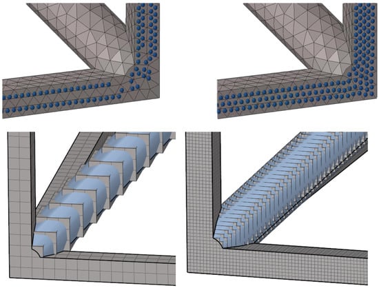
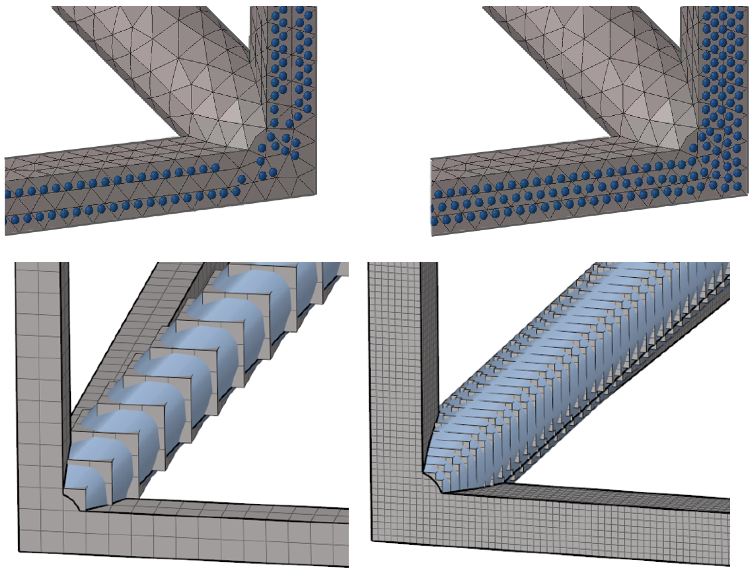
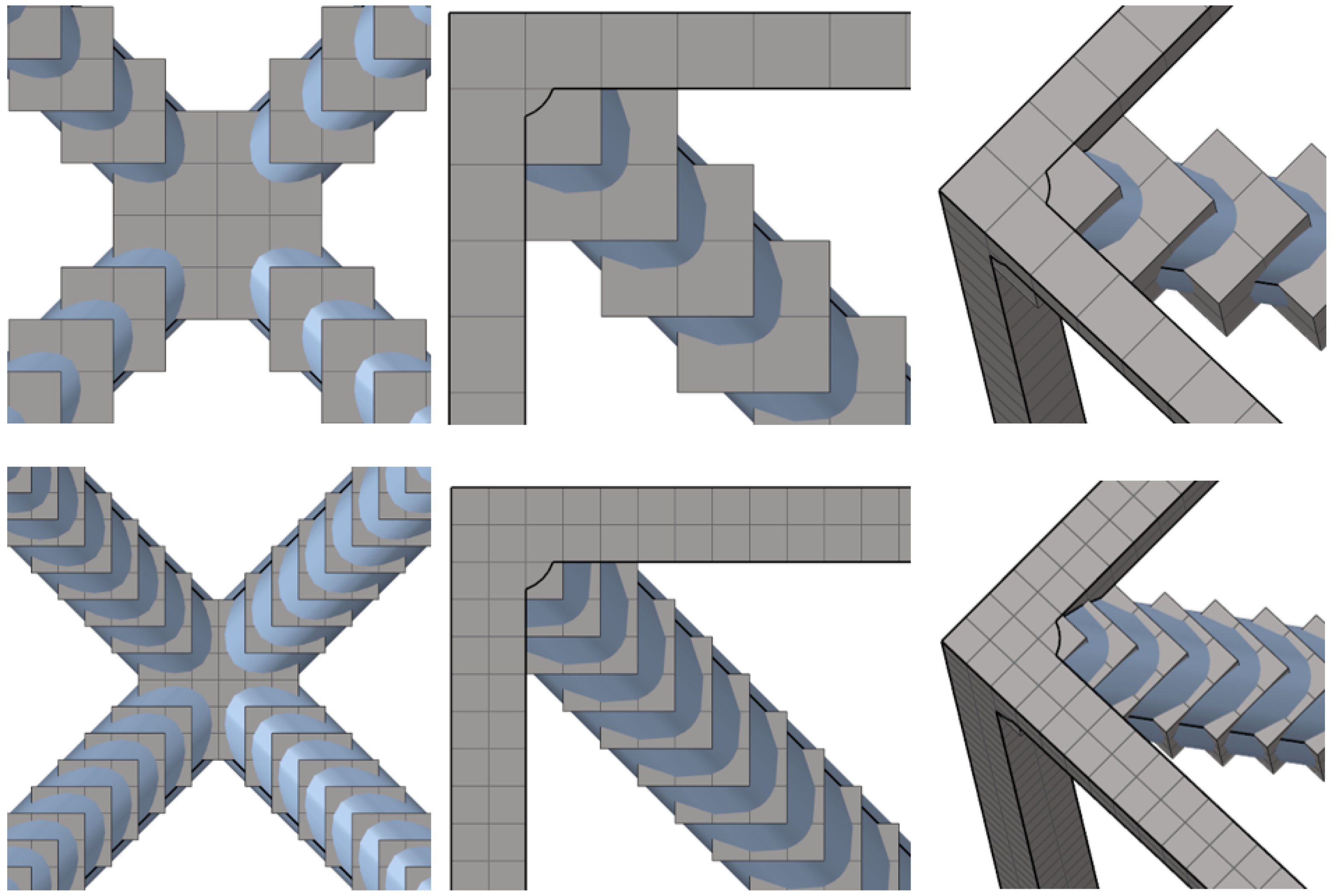
Within numerical models, these imperfections manifest in two distinct scenarios (Figure 1): the deviation of internal nodes (Figure 1 bottom), and the deviation of boundary nodes subjected to Floquet–Bloch periodic constraints (Figure 1 top).
Figure 1.
Influence of two distinct scenarios. Top (type 1): nodes subjected to Floquet-Bloch Theorem at cell boundaries; tolerance: maximum allowed error wrt. element size 5% (left) and 0.1% (right). Bottom (type 2): Geometric deviations within the cell interior; 80 voxels per cell side (left) and 320 voxels per cell side (right).
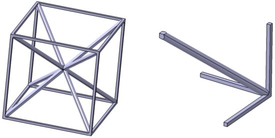
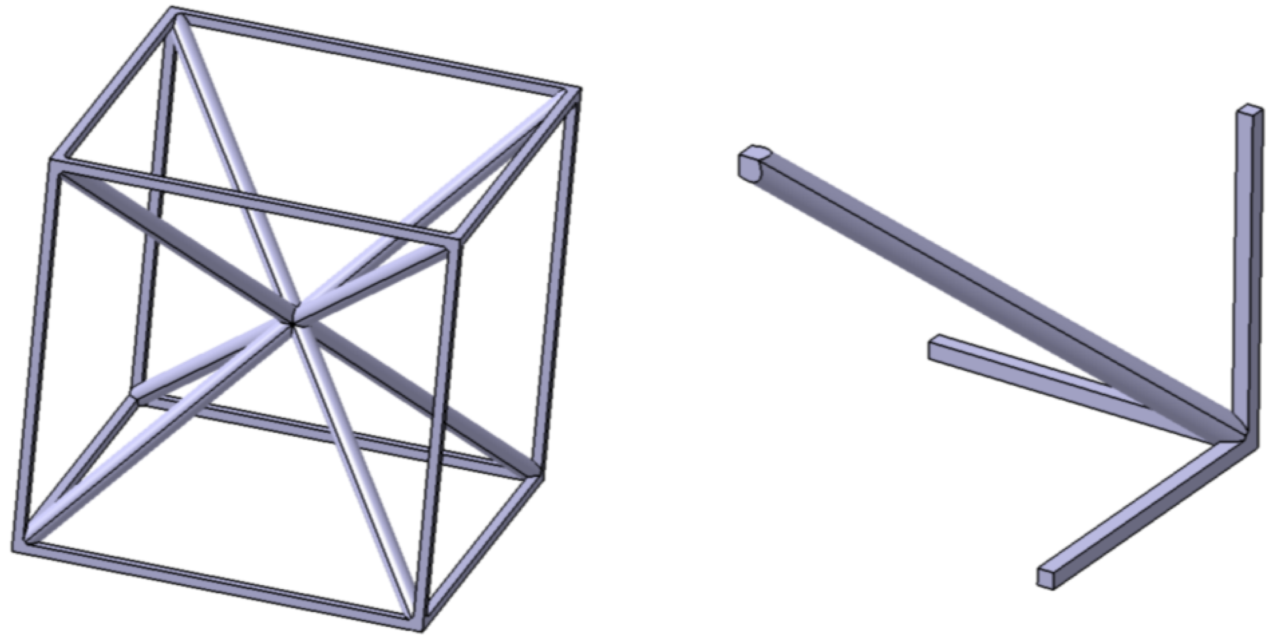
To decouple these two scenarios, a dedicated cubic unit cell with a side length of 20 mm was designed as a case study (Figure 2, left). This cell possesses triple symmetry across the three orthogonal coordinate planes intersecting at its geometric centre, belonging to the space group according to the International Tables for Crystallography [15]. Structurally, the boundaries of the cell are composed of solid parallelepipeds, whereas the interior features cylindrical bars. This specialized geometry enables the generation of a highly conforming mesh, allowing the numerical errors associated with each deviation type to be controlled and analysed independently.
Figure 2.
(Left) Unit Cell Geometry: outer members are parallelogram struts and inner members are cylinders. (Right) One-eighth of the unit cell, used for fitted model.
Even though this specific cell could be modelled with simpler methods, based on the cell symmetry and with the purpose of using generally applicable modelling methods, the fitted mesh has been produced through an automatic mesh with second order solid tetrahedral elements of one-eighth of the unit cell geometry and thereby obtaining the whole cell applying the symmetries (Figure 2, right). The cell geometry has been intentionally designed to be symmetric to facilitate this study, but it must be noted that not every lattice has geometrical symmetries, and therefore the meshing requirements for imposing the boundary conditions are not obtained directly with regular automatic meshing tools.
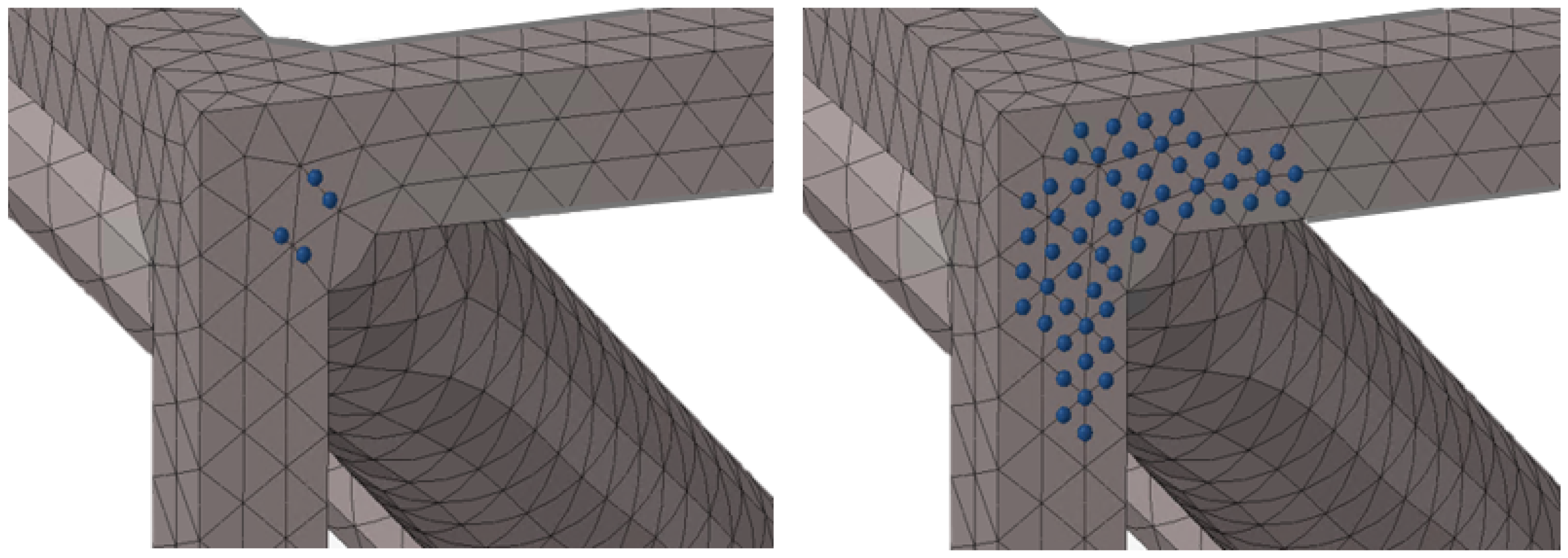
For considering a maximum error at the boundaries, type 1, two different meshers readily available in any commercial finite element software to model any volume have been used for meshing the unit cell, in this case also with second order tetrahedral elements. The two meshing tools selected for this study are commonly employed in the aerospace sector: Altair HyperMesh 2025.1 Tetra Delaunay (mesher A) and MSC Patran v2024.2 Auto TetMesh (mesher B). Once the element size is selected and the geometry is meshed, the non-fitted nodes subjected to periodic boundary conditions that exceed a maximum tolerance value with respect to the element size (parameter also referred as t in Results Section 4.1) have been identified and replaced by nodes that perfectly match the nominal position Figure 3. The new nodes are connected to the surrounding finite-element mesh through multi-point constraint (MPC) equations, whose weighting factors are obtained from the shape functions of the corresponding host elements. In this way, periodic compatibility is enforced without modifying the underlying mesh topology. The boundary geometry remains unchanged with respect to the nominal configuration; therefore, the modelling discrepancy investigated in this work is limited to deviations in the positions of the nodes subjected to periodic boundary conditions.
Figure 3.
Type 1. Induced numerical error at the boundaries. Tolerance: maximum allowed error wrt. element size 15% (left) and 1% (right).
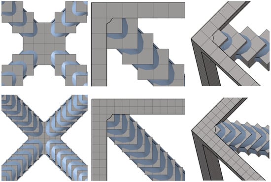
For considering a maximum error within the cell, type 2, a different strategy, also typically available to modellers, has been followed. In this case, the mesh the unit cell is modelled with perfectly cubic hexahedral elements (which we shall refer to in this document as voxels; all having exactly the same size along the lattice). The study has been performed for first and second order elements. These elements can provide a perfect match of the geometry at the boundaries while the error of the inner geometry is related to the size of the voxel: the smaller the voxel size, the better the geometric fidelity of the model (although for large voxel sizes, with the same dimension order of the characteristic length unexpected results may be obtained) Figure 4. With this method, the approximate induced error is half the length of the major diagonal of the voxel.
Figure 4.
Type 2. Overview of meshes generated with voxel cubes, imposing positional error on the interior nodes of each cell. Voxel characteristic sizes of 0.5 mm (top) and 0.25 mm (bottom) correspond to imposed maximum errors of 0.43 mm and 0.22 mm, respectively.
The two types of deviation analysed in this work alter the hypothesis of infinite arrays of metamaterial cells: all the deviations in the position are considered as an infinite repeated deviation due to the imposed boundary conditions. Obviously, this differs from real structures, so that the purpose is to acquire a qualitative knowledge of the different sources of errors that must be considered when simulating the actual dynamic response of lattice-based MMM in a second step simulation. The accurate characterization of these geometric deviations in the response of the metastructure requires the simulation of the real finite geometry without periodic boundary conditions and with the selected unit cell (which is usually selected in a previous trade-off of different single-cells among a collection of diverse options characterized through DD analysis) and their previously characterized deviations applied randomly along all the cells and finally applying the load cases.
4. Impact of Modelling Discrepancies: Results
The results are divided into two types of deviation: numerical errors at the boundaries and numerical errors within the cell. For completeness and to facilitate the reproducibility of the results, Appendix B provides additional information regarding the numerical model, including the mechanical properties of the material, the dimensions of the selected topology, and the chosen path in the Irreducible Brillouin Zone for the wavenumber vector . Furthermore, dispersion diagrams for two representative case studies are included as illustrative examples from which the information discussed in this section is derived.
4.1. Type 1: Numerical Errors at the Boundaries
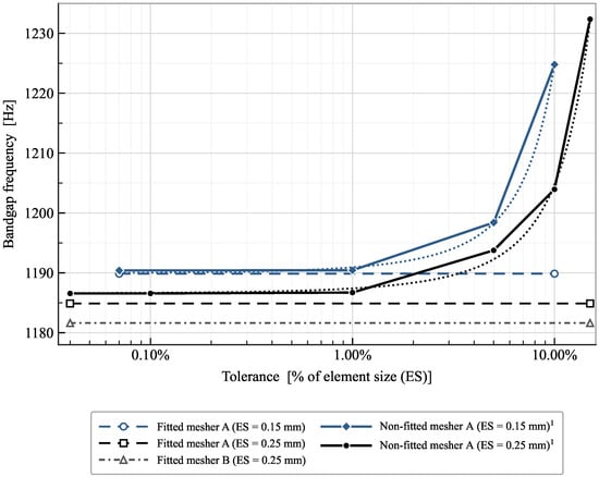
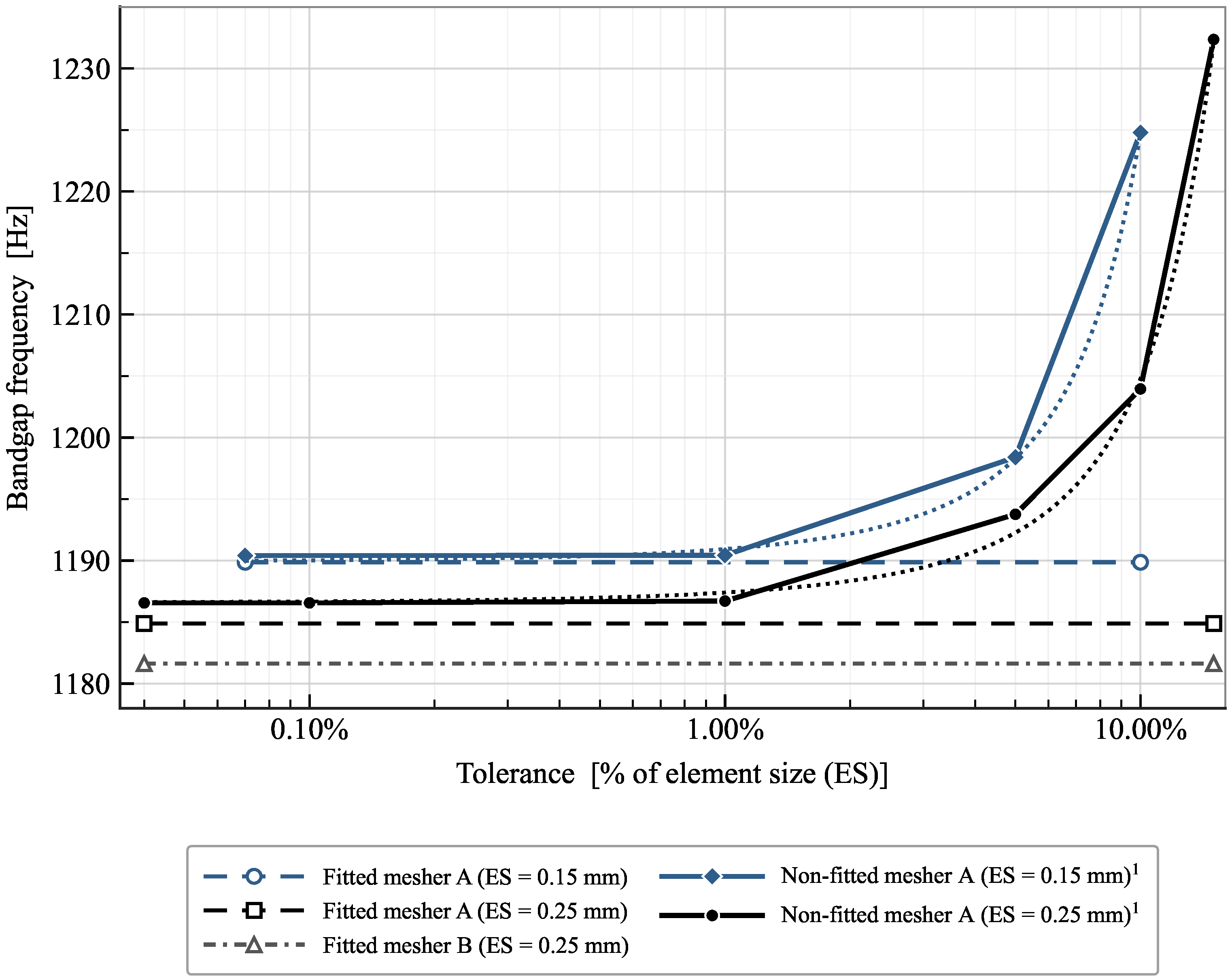
Table 1 summarizes the subcases that have been analysed to assess the impact of the numerical errors at the boundaries. Two different finite element meshers have been used and different prescribed element sizes have been considered. To non-dimesionalise the analysis, the errors (tolerances) were imposed as a percentage of the element size (ES). The combinations considered are marked with ✓ in Table 1. The two element sizes were selected following standard finite element modelling practice, balancing computational cost and geometric representation accuracy. As shown in Figure 5, the fitted reference models produce nearly identical bandgap frequencies for the discretisations considered, indicating that the residual discretisation error is small compared to the modelling discrepancies investigated in this study.
Table 1.
Type 1. Overview of the evaluated subcases for numerical errors at the cell boundaries.
Figure 5.
Type 1: Convergence trend of bandgap width as a function of the tolerance value used. Fitted-mesh results are shown as horizontal lines for clarity (where necessary). 1 Trend lines included as a visual guide to facilitate interpretation.
As outlined in the previous section, fitted models are defined as those in which nodes subject to Floquet–Bloch periodicity conditions are placed exactly at their corresponding locations by construction, leveraging cell symmetry; these models are adopted as the reference solution in this study. Conversely, non-fitted models correspond to meshes automatically generated over the entire geometry, in which only the nodes whose deviation exceeds a prescribed tolerance from their intended positions are replaced prior to imposing the boundary conditions.
The various meshing approaches illustrated in the Figure 5 reveal the unavoidable error inherent to discretization within the FE methodology; consequently, the differences between non-fitted and fitted models can be regarded as negligible for tolerances (X axis) below 1%.
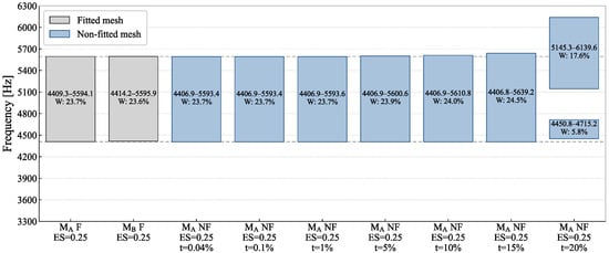
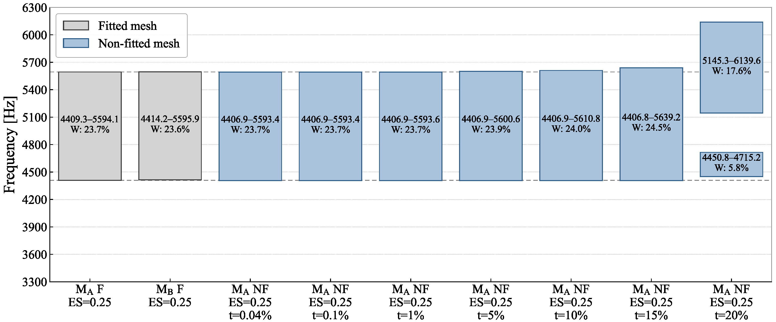
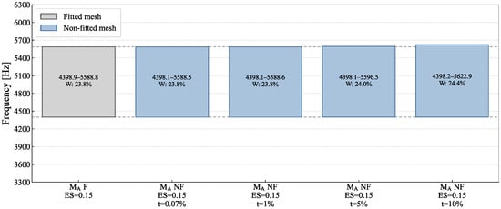
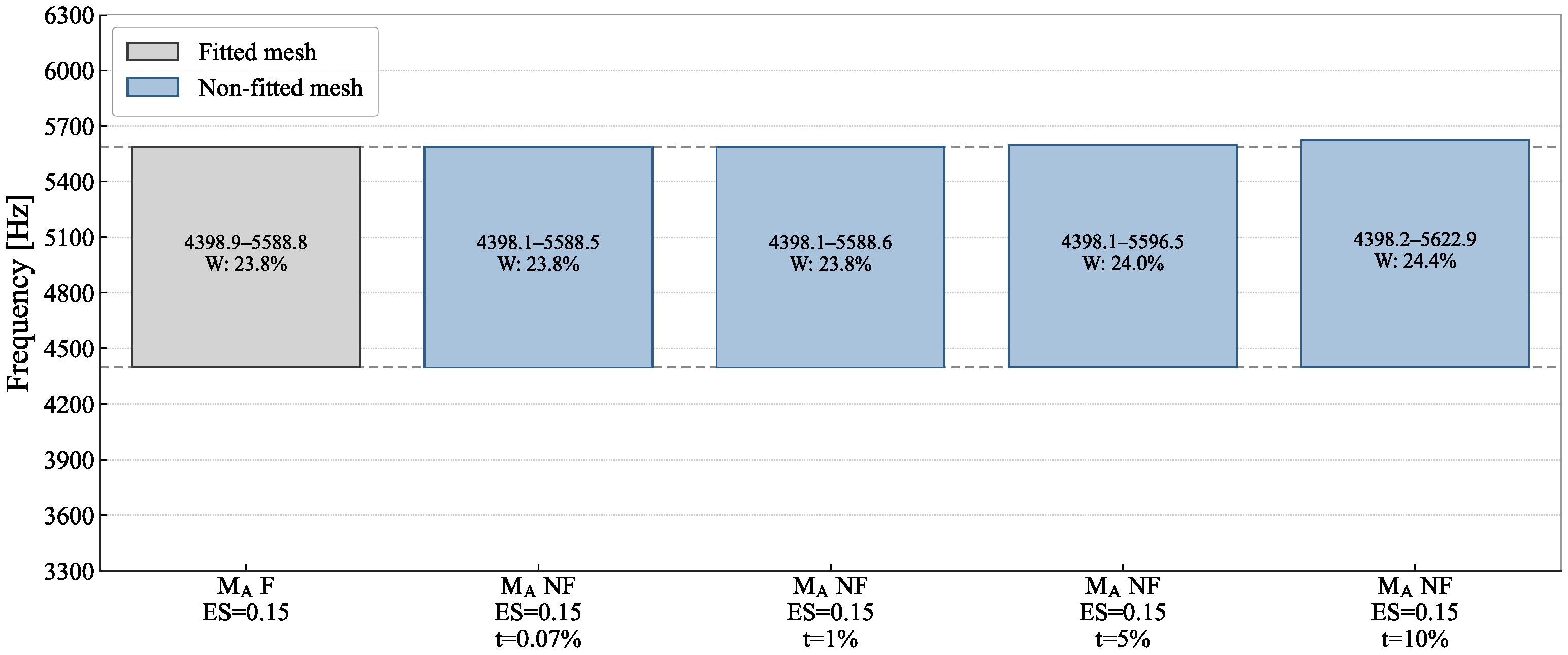
The minima, maxima, and relative band widths (W) of the bandgaps obtained for models with an element size of 0.25 mm are detailed in Figure 6; for clarity, only the bandgap near 5000 Hz is reported. Corresponding results for models with an element size of 0.15 mm are presented in Figure 7.
Figure 6.
Type 1. Bandgap deviation for the different subcases as a function of tolerance value. : mesher A; : mesher B; F: fitted mesh; NF: non-fitted mesh; ES: element Size [mm]; t: tolerance.
Figure 7.
Type 1. Bandgap deviations for the different subcases as a function of tolerance value. : mesher A; F: fitted mesh; NF: non-fitted mesh; ES: element size [mm]; t: tolerance.
4.2. Type 2: Numerical Errors Within the Cell
This section presents the results for the second deviation type studied: errors within the cell. The analysed subcases are summarised in Table 2.
Table 2.
Type 2. Overview of the evaluated subcases for numerical errors within the cell.
The analyses indicate that while the convergence trend approaches the target value, the optimal result still exhibits a discrepancy that exceeds the intrinsic mathematical error of the method. Achieving full agreement with the target would require a more refined model; however, the minimum voxel size was constrained to prevent the total number of degrees of freedom (DOF) from exceeding .
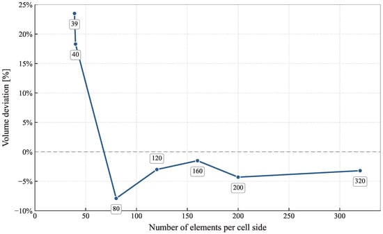
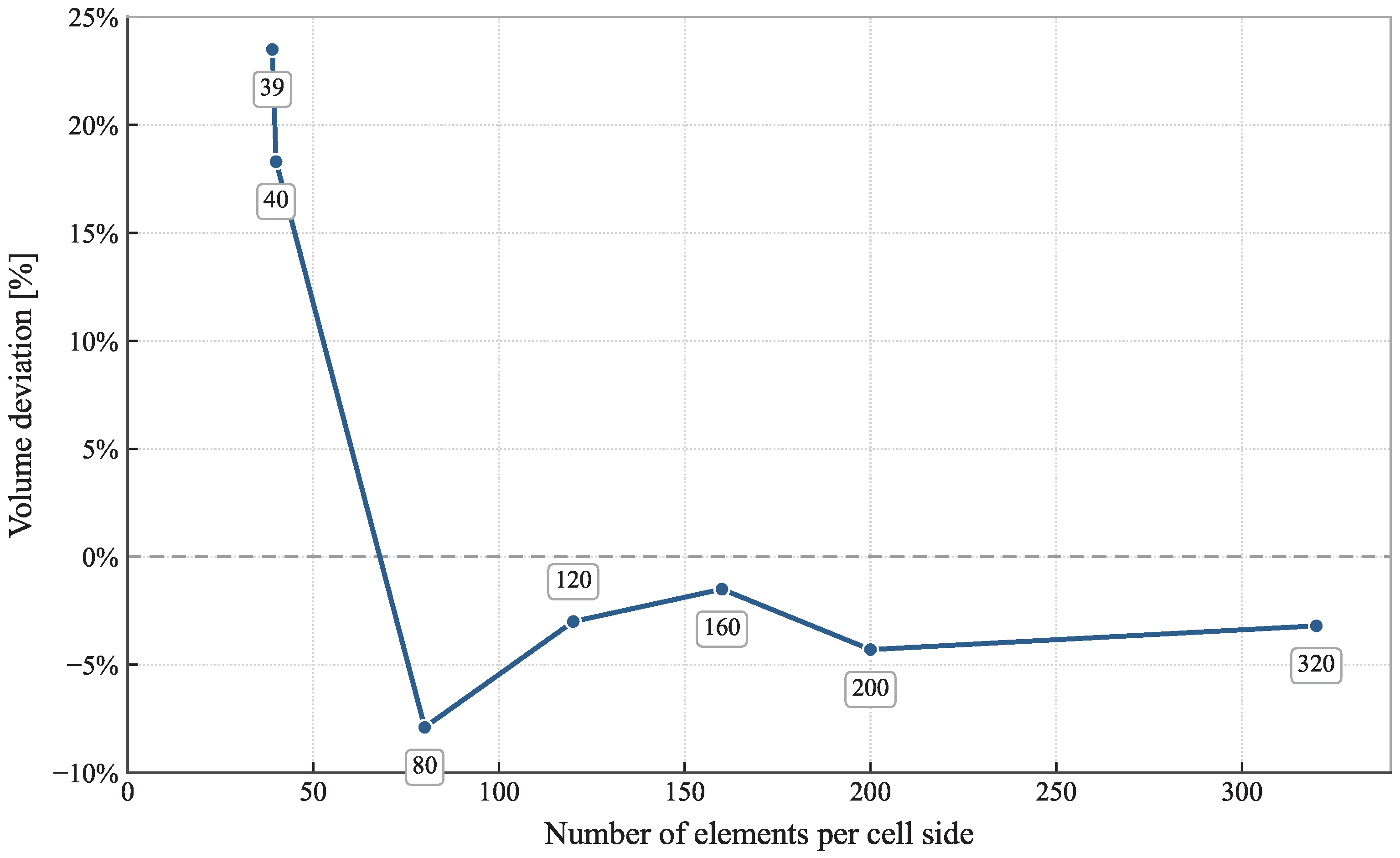
The voxelization algorithm, which activates a voxel whenever material coincides with its nominal center, directly governs the model’s geometric fidelity. As shown in Figure 8, increasing the spatial discretization per cell side (reducing voxel size) enhances agreement with the target volume. However, this convergence trend oscillates, shifting from positive errors in coarser configurations to a negative error in the 80-voxel subcase. This sign inversion critically affects the bandgaps displayed in DD due to the direct impact of mass and stiffness alterations on the structural eigenmodes. Specifically, for this geometry, the geometric overestimation in the inner bars leads to a higher mean bandgap value, effectively compensating for the numerical errors present in the coarser subcases (39 and 40 voxels).
Figure 8.
Type 2: Volume deviation of the mathematical model from the target value (CAD geometry) as a function of the number of elements per cell side.
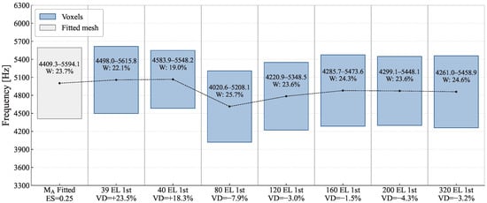
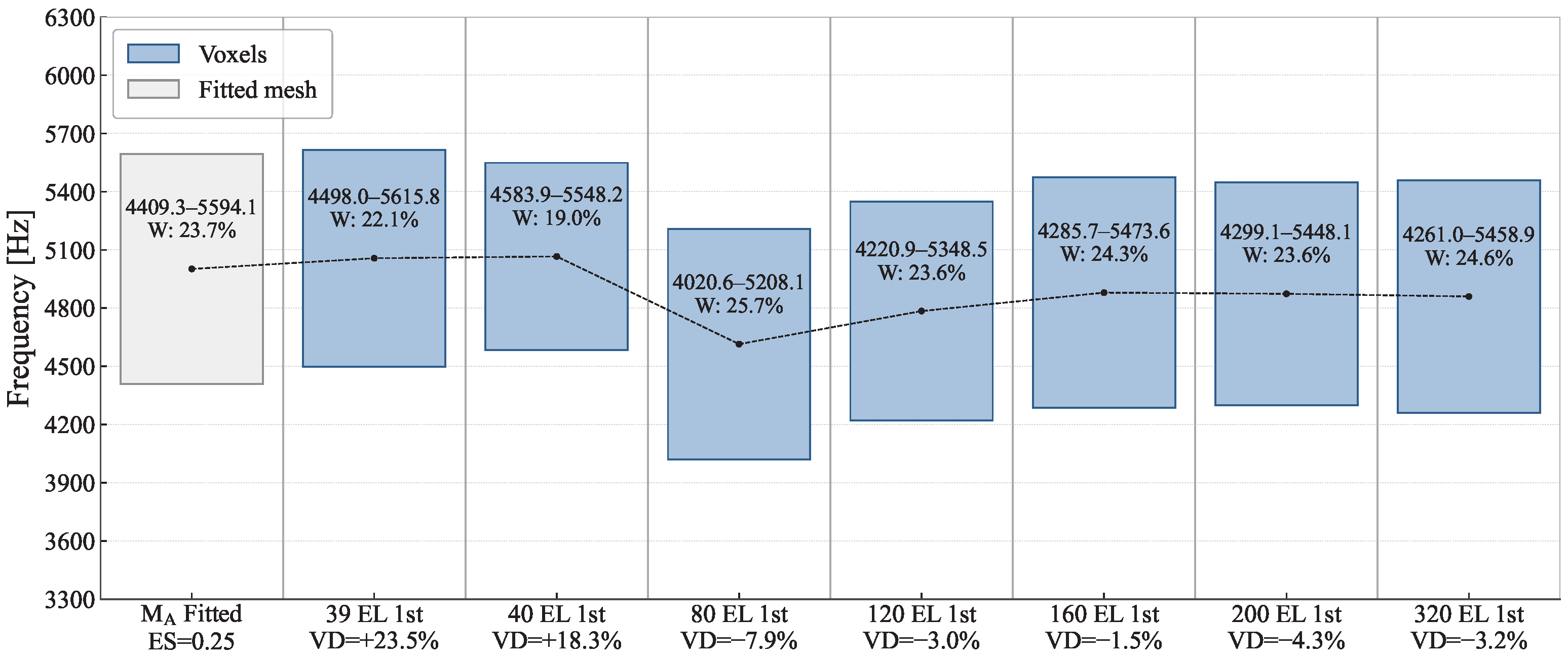
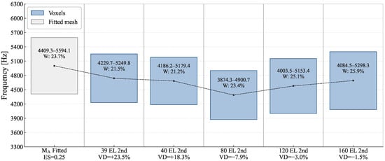
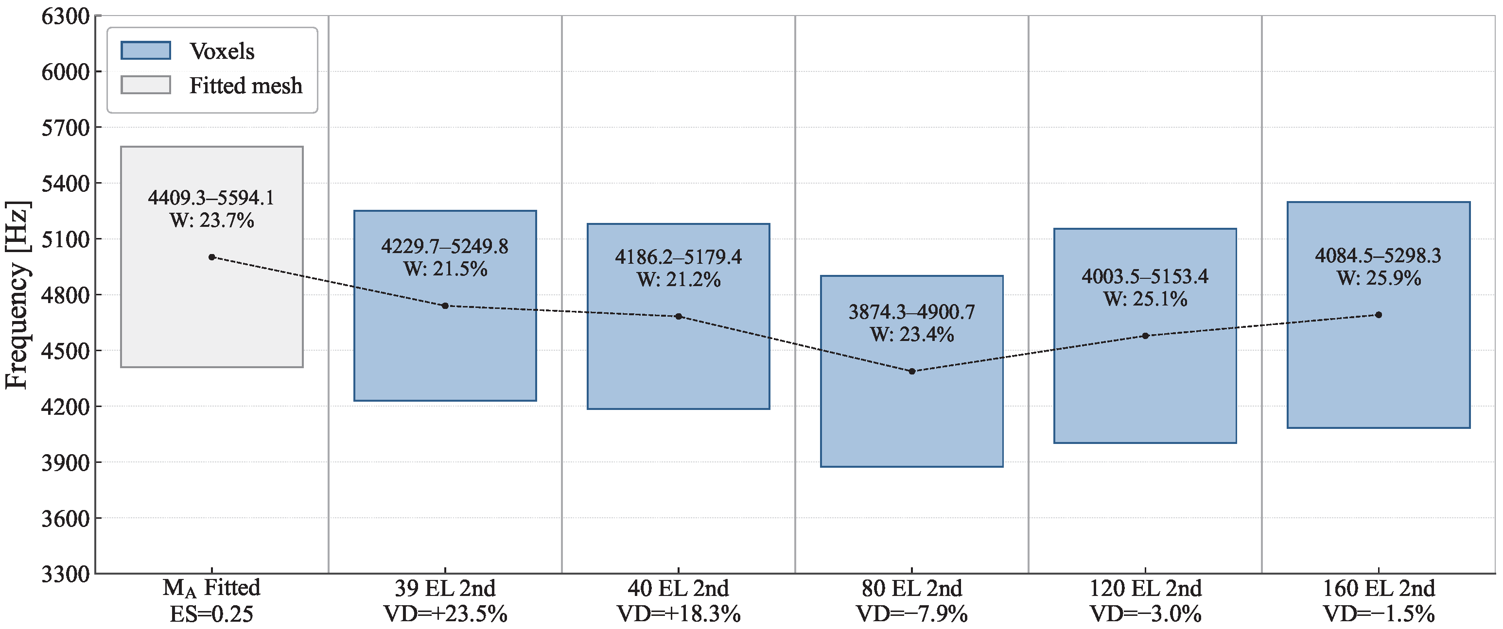
The minima, maxima, and relative band widths (W) of the bandgaps obtained for first and second order voxel models are detailed in figures Figure 9 and Figure 10. As detailed in Appendix B, the fitted reference model exhibits a single isolated bandgap within the analysed frequency range; consequently, no bandgap filtering was applied to the reference solution. To ensure a consistent comparison, minor bandgaps outside the frequency range of interest were excluded, where necessary, from a limited number of models affected by numerical discrepancies, and the defining upper and lower modal branches were verified to correspond to the same eigenmodes across all subcases. As expected, increasing the number of voxels per lattice side enhances the agreement between the calculated bandgap and the target value; the anomalies observed in the coarser models (39 and 40 voxels) stem from the previously discussed volumetric sign deviation. Additionally, a second major effect is identified: the use of second-order elements yields a lower mean bandgap value. This reduction is highly consistent with the inherently lower stiffness characterizing second-order formulations.
Figure 9.
Type 2: Linear hexahedral elements (the fitted model serves as the reference solution analogous to Figure 6, using quadratic tetrahedral elements); ES: element size [mm]; VD: volume deviation wrt. CAD geometry.
Figure 10.
Type 2: Quadratic hexahedral elements (the fitted model serves as the reference solution analogous to Figure 6, using quadratic tetrahedral elements); ES: element size [mm]; VD: volume deviation wrt. CAD geometry.
Given an infinite geometry, the effect of the unit cell selection and the impact on the DD results is shown in Appendix A.
5. Conclusions
In recent years, AM techniques have been increasingly adopted for fabricating lattice-based mechanical metamaterials (MMMs). While AM offers unparalleled advantages for producing intricate geometries, it also introduces inherent manufacturing deviations that directly influence the dynamic response of these structures—specifically the accuracy of phononic bandgaps crucial for vibration isolation. The present work focuses on controlled FE modelling discrepancies and provides new insights into their influence on the reliability of dispersion predictions. Crucially, when MMMs are deployed for vibration attenuation, our findings indicate that unit cells susceptible to internal modelling deviations still deliver satisfactory performance close to their nominal, idealized geometry (Type 2).
Another major outcome of this study directly impacts parametric analyses, which are ubiquitous in lattice-based metastructure research where geometric features are tied to design variables. Because these analyses typically rely on automated computational workflows, researchers must carefully monitor the specific error sources within their numerical models. Notably, node positioning errors at the lattice boundaries (Type 1) must be strictly controlled, whereas errors within the cell interior are far less critical. This distinction justifies the strategic use of coarser meshes in the internal regions of the cell, thereby significantly optimizing the required computational resources without sacrificing global accuracy. Furthermore, the results presented in this work state that different selections of the periodic unit cell produce negligible differences in the predicted bandgaps for the geometry analysed. Nevertheless, minimizing the number of nodes subjected to periodic boundary conditions may still be advantageous from a numerical robustness perspective, as it reduces the sensitivity of the model to boundary-node mismatch errors.
In summary, this work highlights the drastically different effects on dispersion diagrams exerted by two distinct sources of geometric deviation:
- Type 1: Geometric deviations at cell boundaries. Where periodic boundary conditions are enforced, numerical convergence to the true solution is highly sensitive to node placement. Here, accurate dispersion characteristics are achieved only when the maximum allowable positioning error of the boundary nodes remains below 1% of the local element size.
- Type 2: Geometric deviations within the cell interior. The primary results demonstrate that internal spatial errors up to 50% of the characteristic strut length can still yield acceptable results for initial design screening, provided that the total volume deviation of the unit cell is maintained below 20%. These thresholds should be regarded as practical guidelines derived from the present case study and may require further validation before being extrapolated to other lattice topologies, relative densities, material systems, or bandgap-generation mechanisms.
Author Contributions
Conceptualization, J.G.-M.; methodology, I.M.-T., P.P.T. and J.G.-M.; software, I.M.-T. and K.V.B.; validation, P.P.T.; formal analysis, K.V.B. and P.P.T.; investigation, I.M.-T.; data curation, P.P.T.; writing—review and editing, I.M.-T., K.V.B., P.P.T., J.G.-M. and F.J.M.; visualization, P.P.T., J.G.-M. and F.J.M.; supervision, J.G.-M. and F.J.M.; funding acquisition, J.G.-M. and F.J.M. All authors have read and agreed to the published version of the manuscript.
Funding
This research received funding from coordinated project BRISAS (PID2024-155747OA-C33), supported by MICIU/AEI/10.13039/501100011033, and by “ERDF A way of making Europe”. This research received funding from the European Union’s Horizon 2020 Marie Sklodowska-Curie Actions—Innovative European Training Networks under grant agreement No 956401 (XS-Meta).
Institutional Review Board Statement
Not applicable.
Data Availability Statement
Selected FE models are available at https://doi.org/10.5281/zenodo.20560657 (accessed on 27 July 2026). For type 1 of deviation: unit cell with element size of 0.25 mm, fitted and non-fitted. For type 2 of deviation: unit cell with 40 voxels per side (second order hexahedral elements), original, variant 1 and variant 2 geometries. Additional data will be made available on request.
Acknowledgments
During the preparation of this study, the authors used Claude versions 4.6, 4.7, and 4.8 to assist with the generation and modification of Python 3.12 scripts supporting the research workflow, including the creation and formatting of curves and graphical outputs, as well as the parametric modification of computational models. Gemini 1.5 has been used to correct and enhance English text. The authors have reviewed and edited the output and take full responsibility for the content of this publication.
Conflicts of Interest
The authors declare no conflicts of interest.
Abbreviations
The following abbreviations are used in this manuscript:
| AM | Additive manufacturing |
| CAD | Computer-aided design |
| DDs | Dispersion diagrams |
| DOF | Degrees of freedom |
| ES | Element size |
| FE | Finite element |
| IBZ | Irreducible Brillouin Zone |
| MMMs | Mechanical metamaterials |
| VD | Volume deviation |
Appendix A. Unit Cell Selection
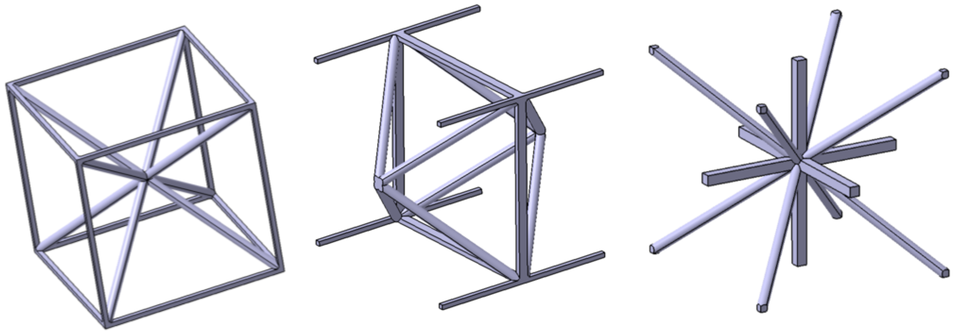
The selection of boundaries for a specific geometry is not unique as different unit cells can be selected offering an identical infinite geometry. For the selected unit cell, three variants (Figure A1 and Figure A2) have been studied in order to validate that this selection has no impact on the obtained bandgap results.
Figure A1.
Three variants of the unit cell selection generating a final identical infinite geometry. From left to right: original; variant 1; variant 2.
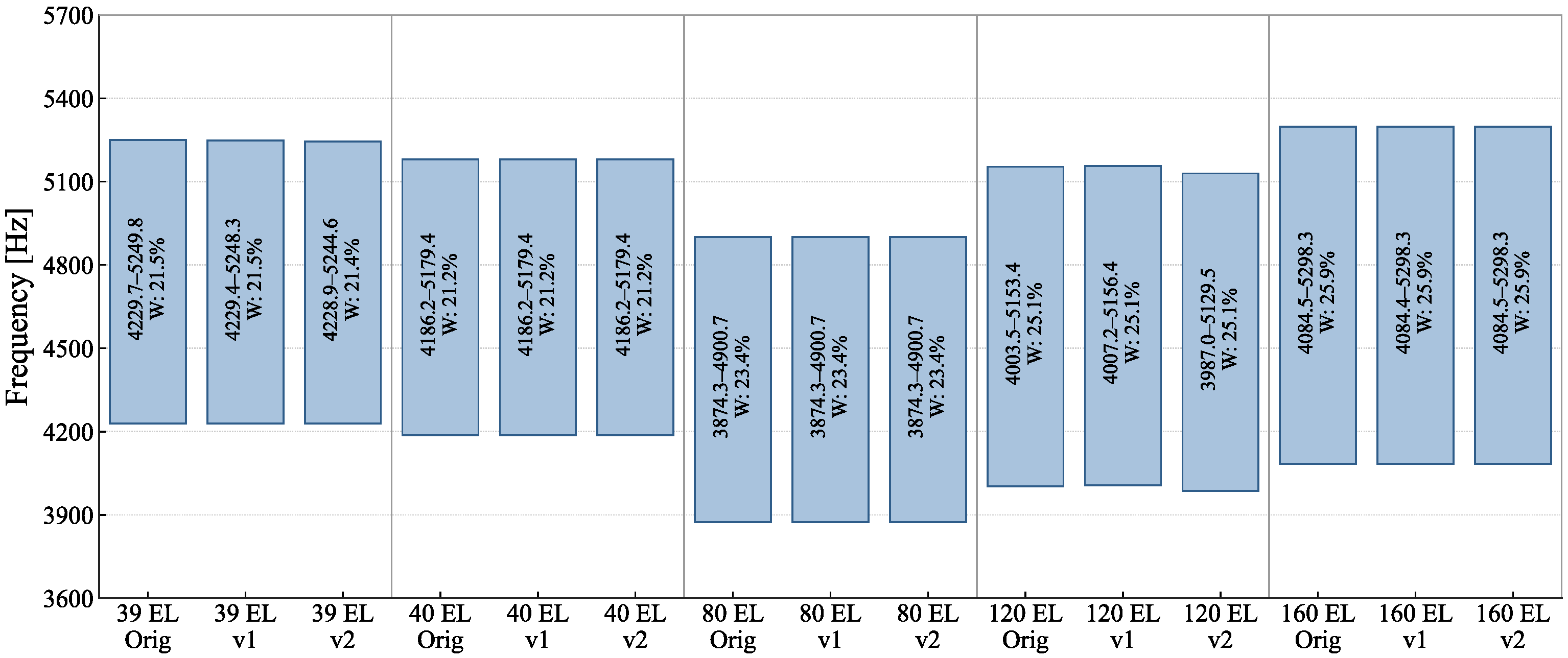
The associated FE models to the different unit cells is equivalent (the same number and type of elements is used in all cases), so that the main difference relies on the periodic boundary conditions applied. The differences in the obtained bandgaps are negligible as shown in Figure A3.
Figure A2.
FE models associated to the three variants of the unit cell selection. From left to right: original; variant 1; variant 2.
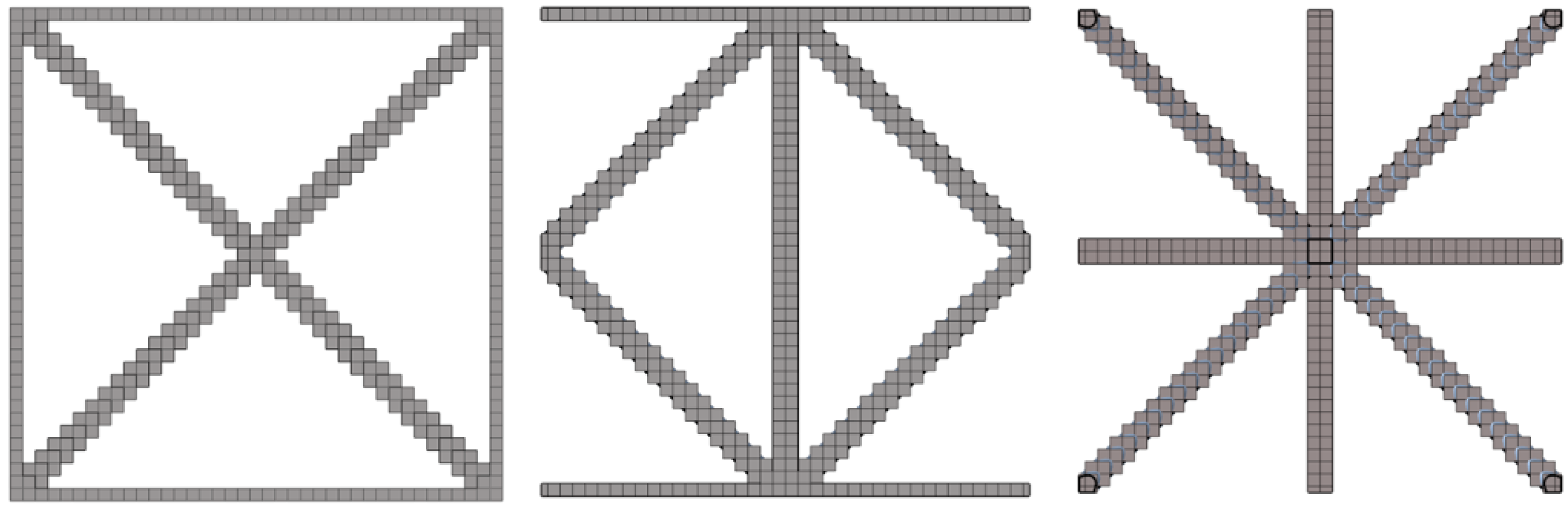
Figure A3.
Bandgaps associated to the three variants of the unit cell selection.
Appendix B. Numerical Model Parameters and Dispersion Diagrams
Additional information on the numerical models used in this study is provided to facilitate the reproducibility of the reported results. The main parameters of the model are summarised, including material properties, geometric dimensions, representative mesh characteristics, and numbers of degrees of freedom, together with the path and sampling considered in the Irreducible Brillouin Zone for the wavenumber vector . In addition, representative dispersion diagrams for two case studies are included to illustrate the data from which the analyses presented in the main text are derived.
Selected FE models are available through the repository referenced in the Data Availability Statement, from which the corresponding unit-cell geometries, material properties, and eigenmode computation parameters can be obtained. The unit cell considered for this study is a cubic lattice with a characteristic side length of 20 mm. The lattice is composed of edge struts with a square cross-section of , and diagonal struts with a circular cross-section of diameter extending from the cube centre to each of its vertices.
The material properties adopted in the FE models are reported in Table A1. These properties are representative of a polymeric material for additive manufacturing.
Table A1.
Material properties of the thermoplastic polymeric material employed in the finite-element models available in the repository.
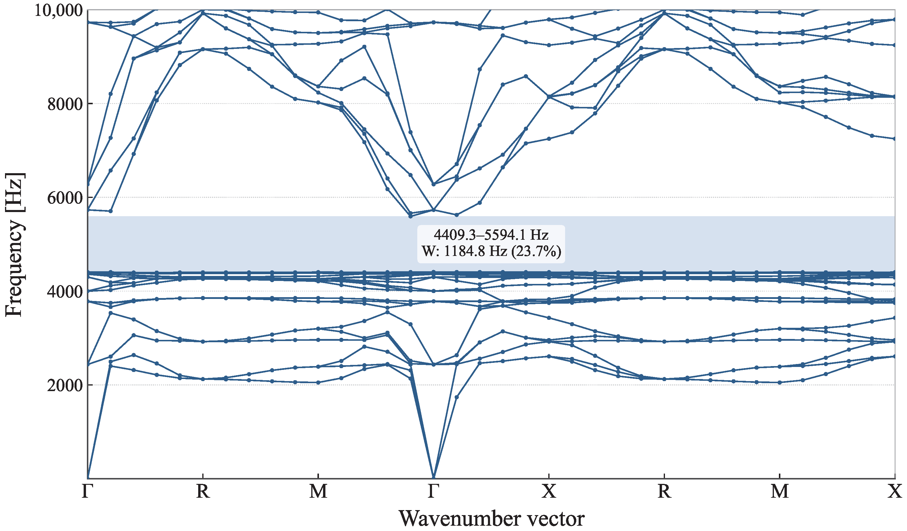
The dispersion diagram for the reference solution considered in this study is presented in Figure A4 as a representative sample of all the data used for this study. The path followed has been selected to explore all the edges of the IBZ of a cubic lattice: –R–M––X–R-M–X. The wavevector-space coordinates in the Bouckaert-Smoluchowski-Wigner (BSW) notation and the units per meter in the reciprocal base are , and . For the computation of the dispersion relations, four equally spaced sampling points were considered between each pair of adjacent high-symmetry points in the selected wavenumber vector path, allowing for the construction of the corresponding dispersion branches. A total of 100 complex eigenmodes of the undamped system were obtained for each value of the wavenumber vector , covering frequencies up to approximately 36 kHz. Within this frequency range, only a single bandgap was identified for the fitted reference model. However, only the modes below 10 kHz are shown in the dispersion diagrams for clarity. This frequency range corresponds approximately to the first 30 modes and encompasses the bandgap analysed in the present work. The three lowest branches in the dispersion diagrams correspond to rigid-body modes of the unit cell.
Figure A4.
Dispersion diagram for the fitted mesh, mesher A, element size 0.25 mm.
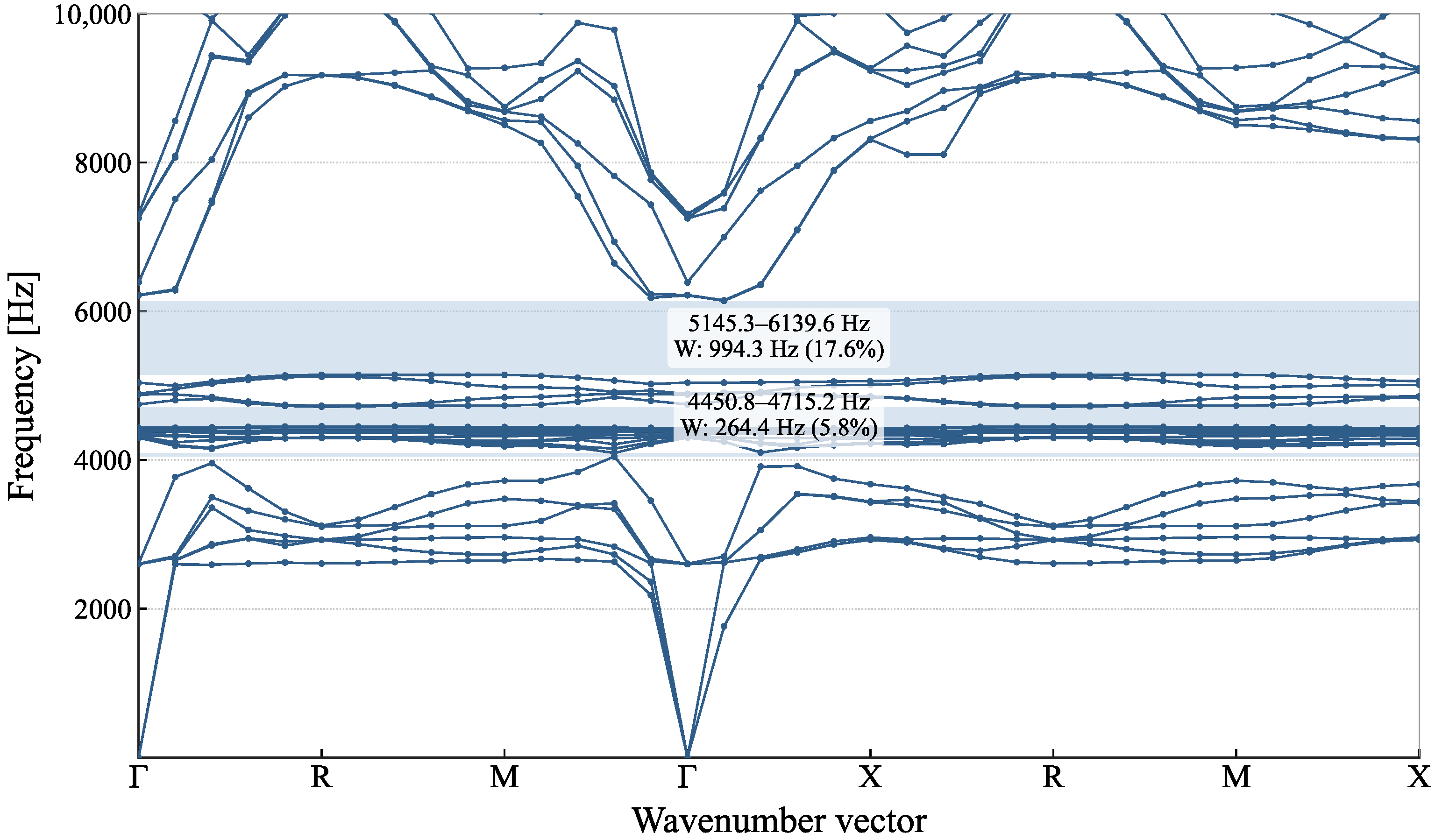
The dispersion diagram for the selected case exhibiting the largest Type 1 deviation is shown in Figure A5. To enable a reliable comparison with the reference solution, the mode shapes were inspected at several high-symmetry points along the selected wave vector path. The two bandgaps reported herein were identified based on the similarity between the lower band-edge mode at 4450 Hz and the upper band-edge mode at 6140 Hz and their counterparts in the reference model. The bandgap splitting exhibited by this case motivated its exclusion from Figure 5, as the results for tolerances up to 10% already capture the rapidly increasing trend in bandgap width error.
Figure A5.
Dispersion diagram for the non-fitted mesh, mesher A, element size 0.25 mm, tolerance = 20%.
References
- Elias, S.; Beer, M. A novel quantum-theory-based optimization of tuned mass dampers for structural vibration control. Comp. Struct. 2025, 319, 108013. [Google Scholar] [CrossRef] [Scilit]
- Sigalas, M.M.; Economou, E.N. Elastic and Acoustic Wave Band Structure. J. Sound Vib. 1992, 158, 377–382. [Google Scholar] [CrossRef] [Scilit]
- Sheng, P.; Zhang, X.X.; Liu, Z.; Chan, C.T. Locally Resonant Sonic Materials. Phys. B 2003, 338, 201–205. [Google Scholar] [CrossRef] [Scilit]
- Meier, T.; Korakis, V.; Blankenship, B.W.; Lu, H.; Kyriakou, E.; Papamakarios, S.; Vangelatos, Z.; Yildizdag, M.E.; Zyla, G.; Xia, X.; et al. Scalable Phononic Metamaterials: Tunable Bandgap Design and Multi-Scale Experimental Validation. Mater. Des. 2025, 252, 113778. [Google Scholar] [CrossRef] [Scilit]
- Jiang, W.; Yin, G.; Xie, L.; Yin, M. Multifunctional 3D Lattice Metamaterials for Vibration Mitigation and Energy Absorption. Int. J. Mech. Sci. 2022, 233, 107678. [Google Scholar] [CrossRef] [Scilit]
- Liu, L.; Kamm, P.; García-Moreno, F.; Banhart, J.; Pasini, D. Elastic and Failure Response of Imperfect Three-Dimensional Metallic Lattices: The Role of Geometric Defects Induced by Selective Laser Melting. J. Mech. Phys. Solids 2017, 107, 160–184. [Google Scholar] [CrossRef] [Scilit]
- Mencik, J.-M.; Duhamel, D. A Wave Finite Element-Based Approach for the Modeling of Periodic Structures with Local Perturbations. Finite Elem. Anal. Des. 2016, 121, 40–51. [Google Scholar] [CrossRef] [Scilit]
- Zhang, H.; Mahabadi, R.K.; Rudin, C.; Guilleminot, J.; Brinson, L.C. Uncertainty Quantification of Acoustic Metamaterial Bandgaps with Stochastic Material Properties and Geometric Defects. Comput. Struct. 2024, 305, 107511. [Google Scholar] [CrossRef] [Scilit]
- Al Ba’ba’a, H.; Nandi, S.; Singh, T.; Nouh, M. Uncertainty Quantification of Tunable Elastic Metamaterials Using Polynomial Chaos. J. Appl. Phys. 2020, 127, 015102. [Google Scholar] [CrossRef] [Scilit]
- Walker, O.; Roland, T.; Favier, D.; Egele, A.; Heymann, M.; Stubenrauch, C. Mechanical Properties of Architected Polymer Lattice Materials: A Comparative Study of Additive Manufacturing and CAD Using FEM and μ-CT. Adv. Funct. Mater. 2026, 36, e12520. [Google Scholar] [CrossRef] [Scilit]
- Kai, Y.; Dhulipala, S.; Sun, R.; Lem, J.; DeLima, W.; Pezeril, T.; Portela, C.M. Dynamic Diagnosis of Metamaterials through Laser-Induced Vibrational Signatures. Nature 2023, 623, 514–521. [Google Scholar] [CrossRef] [Scilit] [PubMed]
- Beniwal, S.; Bose, R.K.; Krushynska, A.O. Characterizing Dissipative Elastic Metamaterials Produced by Additive Manufacturing. J. Vis. Exp. 2024, 208, e66898. [Google Scholar] [CrossRef] [Scilit] [PubMed]
- Maurin, F.; Claeys, C.; Deckers, E.; Desmet, W. Probability That a Band-Gap Extremum Is Located on the Irreducible Brillouin-Zone Contour for the 17 Different Plane Crystallographic Lattices. Int. J. Solids Struct. 2018, 135, 26–36. [Google Scholar] [CrossRef] [Scilit]
- Vera-Rodríguez, G.; Moreno-Corrales, L.; Marín-González, I.; Barba, D.; Montáns, F.J.; Sanz-Gómez, M.Á. Incorporation of Defects in Finite Elements to Model Effective Mechanical Properties of Metamaterial Cells Printed by Selective Laser Melting. Sustainability 2024, 16, 1167. [Google Scholar] [CrossRef] [Scilit]
- Hahn, T. (Ed.) International Tables for Crystallography: Space-Group Symmetry, 1st ed.; International Union of Crystallography: Chester, UK, 2006; Volume A. [Google Scholar] [CrossRef] [Scilit]

Disclaimer/Publisher’s Note: The statements, opinions and data contained in all publications are solely those of the individual author(s) and contributor(s) and not of MDPI and/or the editor(s). MDPI and/or the editor(s) disclaim responsibility for any injury to people or property resulting from any ideas, methods, instructions or products referred to in the content. |
© 2026 by the authors. Licensee MDPI, Basel, Switzerland. This article is an open access article distributed under the terms and conditions of the Creative Commons Attribution (CC BY) license.