Wind Pressure Coefficient Distribution and Shape Factor of Wind Load of Plastic Greenhouse Cluster in Valley Terrain Based on CFD Simulation

Abstract

Understanding wind load characteristics of greenhouse clusters in valley terrain is essential for ensuring structural safety in high-altitude agricultural regions. This study investigates the wind pressure coefficient distribution of plastic greenhouse clusters located in a representative high-altitude valley region (Case sourced from Tibet, China) using computational fluid dynamics simulations. Numerical models incorporating realistic topographic features and representative cluster layouts (2 × 3, 3 × 3, and 3 × 5) were established to evaluate surface wind pressure coefficient distribution and wind load shape factors. The results indicate that valley terrain modifies the incoming wind field through terrain-induced acceleration and possible flow separation. Compared with flat-terrain assumptions, wind load shape factors show noticeable deviations, particularly in windward, roof, and leeward regions. First-row and peripheral greenhouses consistently experience the largest wind loads due to direct wind exposure, while interior greenhouses are significantly influenced by aerodynamic shielding effects from upstream structures. As cluster density increases, shielding effects reduce wind pressure magnitude and result in a more stable pressure distribution within the interior region of the cluster. The correction coefficient derived in this study should be regarded as site-specific indicators for the selected valley terrain, greenhouse layout, and wind direction, rather than as generally applicable design coefficients.

1. Introduction

Plastic greenhouses are widely used in modern facility agriculture due to their low construction cost, ease of installation, and favorable thermal insulation performance. In high-altitude and cold-region environments such as the Tibetan Plateau, plastic greenhouses play an important role in ensuring stable crop production and improving agricultural productivity. In fact, global mountainous regions—such as the Alps in Europe and the Himalayas in Asia—are home to millions of people, making these greenhouses indispensable for ensuring local food security.

However, plastic greenhouses are lightweight structures with relatively low stiffness and limited resistance to wind loads. Compared with conventional buildings, greenhouse envelope systems are more sensitive to external wind pressure, and structural damage caused by strong wind events occurs frequently in mountainous regions. Therefore, understanding wind load characteristics and wind pressure coefficient distribution is essential for ensuring the structural safety and reliability of plastic greenhouses.

Wind characteristics in valley terrain differ significantly from those over flat terrain because of the influence of complex topography. Therefore, the investigation of wind characteristics in valley regions is an important prerequisite for accurately evaluating wind loads acting on structures located in these challenging mountainous environments.

Previous studies have investigated wind field characteristics in complex terrain using both experimental and numerical approaches. Bowen and Lindley [1] experimentally studied wind speed and turbulence characteristics over escarpment terrain and demonstrated that terrain geometry significantly modifies wind profiles near the ground surface. Kwon et al. [2] conducted wind tunnel tests on wind pressure coefficients of single-span greenhouses built on reclaimed coastal land and demonstrated that terrain-specific wind characteristics greatly affect the structural wind load distribution. Maraveas [3] reviewed published wind pressure coefficients for greenhouse structures and compared them with theEuropean design code provisions, concluding that current evidence is insufficient to justify revisions of the standard, although discrepancies were identified in local regions and complex configurations. Xu et al. [4,5] applied numerical simulation methods to study wind field characteristics in valley environments and showed that terrain effects significantly influence local wind speed distribution.

Also, to determine wind loads acting on greenhouse structures, it is necessary to further investigate wind pressure coefficient distribution on structural surfaces. Wind pressure characteristics of buildings are commonly studied using field measurements [6,7,8,9,10,11], wind tunnel experiments [12,13,14,15], and computational fluid dynamics (CFD) simulations [16,17,18]. Castro and Robins [19] conducted experimental investigations of the flow around a surface-mounted cube, providing benchmark data for wind pressure research on low-rise structures. Holmes [20] systematically summarized wind loading theory and emphasized the importance of wind pressure coefficients in structural wind-resistant design.

Garcia et al. [21] developed a numerical model of a multi-span greenhouse and evaluated its structural response under wind loading based on existing wind loading standards, with the results compared against the corresponding code values. The study showed that finite element analysis is an effective tool for structural assessment and optimization. Kim et al. [22] employed large eddy simulation (LES) to predict both mean and peak wind pressure coefficients on single-span greenhouses; the results showed that LES outperformed conventional RANS models, particularly in capturing local peak suctions. Blocken [23] reviewed the development of computational wind engineering and highlighted the advantages of CFD methods in resolving complex airflow structures around buildings. In addition, previous studies have demonstrated that the wind pressure coefficient distribution on greenhouse surfaces is significantly affected by greenhouse geometry, structural layout, and span number [24,25]. Furthermore, complex terrain factors, such as mountainous topography, wind direction, and mountain distance, can substantially modify local wind fields and alter the wind load characteristics acting on greenhouse structures [26,27]. These studies provide important references for evaluating wind load characteristics of greenhouses under different structural and environmental conditions.

The above studies have investigated wind pressure characteristics of individual greenhouses and wind field characteristics in complex terrain. Limited research has examined the combined influence of valley terrain and greenhouse cluster arrangements on wind pressure coefficient distribution. When multiple greenhouses are arranged in groups, aerodynamic interference between adjacent structures may produce shielding effects, wake interaction, and vortex superposition, resulting in significant spatial variation in wind pressure on different greenhouse surfaces. The interaction between terrain-induced flow distortion and group interference may further increase the complexity of wind load distribution. Therefore, investigation of wind pressure characteristics of greenhouse clusters in valley terrain is necessary for improving wind-resistant design methods and optimizing greenhouse layout schemes in mountainous regions.

To address this research issue, this study investigates wind pressure coefficient distribution characteristics and wind load shape factors (area-averaged wind pressure coefficient) of plastic greenhouse clusters located in valley terrain in Tibet, China. A three-dimensional CFD model incorporating realistic mountainous topography and multiple greenhouse layout configurations is established to simulate airflow behavior and surface wind pressure coefficient distribution under typical wind conditions. Three representative greenhouse cluster arrangements (2 × 3, 3 × 3, and 3 × 5) are analyzed to evaluate the influence of terrain effects and group interference on wind load characteristics. Considering the geographic location of the study region, the wind load evaluation is conducted based on the Chinese wind loading code to satisfy local engineering design requirements. The results provide theoretical support for wind-resistant design and layout optimization of greenhouse clusters in mountainous regions and contribute to improving understanding of aerodynamic interaction mechanisms of lightweight structures subjected to complex wind environments.

Because wind fields in complex terrain are strongly dependent on local topography and structure location, the correction coefficients proposed here are intended for the selected case and should not be directly generalized to other valley environments without site-specific verification.

2. Methodology Overview

The objective of this study is to investigate the influence of valley terrain on the wind load characteristics of plastic greenhouse clusters and to provide a scientific basis for wind-resistant structural design in mountainous regions. The research framework integrates terrain modeling, computational fluid dynamics (CFD) simulation, and aerodynamic analysis to systematically evaluate wind pressure coefficient distributions under realistic environmental conditions.

The methodological strategy is based on the principle that wind loads acting on greenhouse structures are governed by the interaction between incoming flow characteristics and structural configuration. In valley terrain, topographic features significantly modify the upstream wind field through flow acceleration, separation, and turbulence variation. These terrain-induced effects influence the spatial distribution of wind pressure on greenhouse surfaces and may alter the magnitude of wind load shape factors compared with those obtained under flat-terrain assumptions.

To capture these coupled effects, a numerical simulation framework incorporating realistic topography and representative greenhouse cluster layouts is established. The approach enables evaluation of both terrain-induced wind field distortion and aerodynamic interference among multiple greenhouse structures. By comparing wind pressure coefficient distributions across different layout configurations, the combined influence of terrain-modified inflow and greenhouse-array arrangement can be evaluated.

The research framework consists of three main components:

• Terrain modeling, which reconstructs realistic valley topography using digital elevation data to reproduce the spatial characteristics of the wind environment in mountainous regions.
• The terrain-scale and greenhouse-scale simulations were linked using a one-way transfer strategy, as described in Section 4.4.1.
• Aerodynamic analysis of greenhouse clusters, which determines surface wind pressure coefficient distribution and wind load shape factors for different cluster configurations, enabling quantitative evaluation of the influence of terrain effects and group interference on wind load characteristics.

3. Layout and Dimensions of Greenhouse Cluster

3.1. Geometric Parameters and Surface Partitioning of a Single Plastic Greenhouse

The reference greenhouse model adopted in this study represents a commonly used single-span plastic greenhouse structure in China. The geometric parameters of the greenhouse are defined as follows: the length L, span b, and height H_G of the greenhouse are 44 m, 7 m, and 3.5 m, respectively; the shoulder height H_L is 1.6 m, corresponding to a rise-to-span ratio of 0.2714.

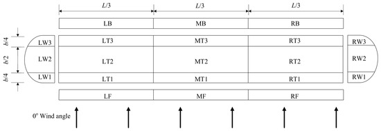
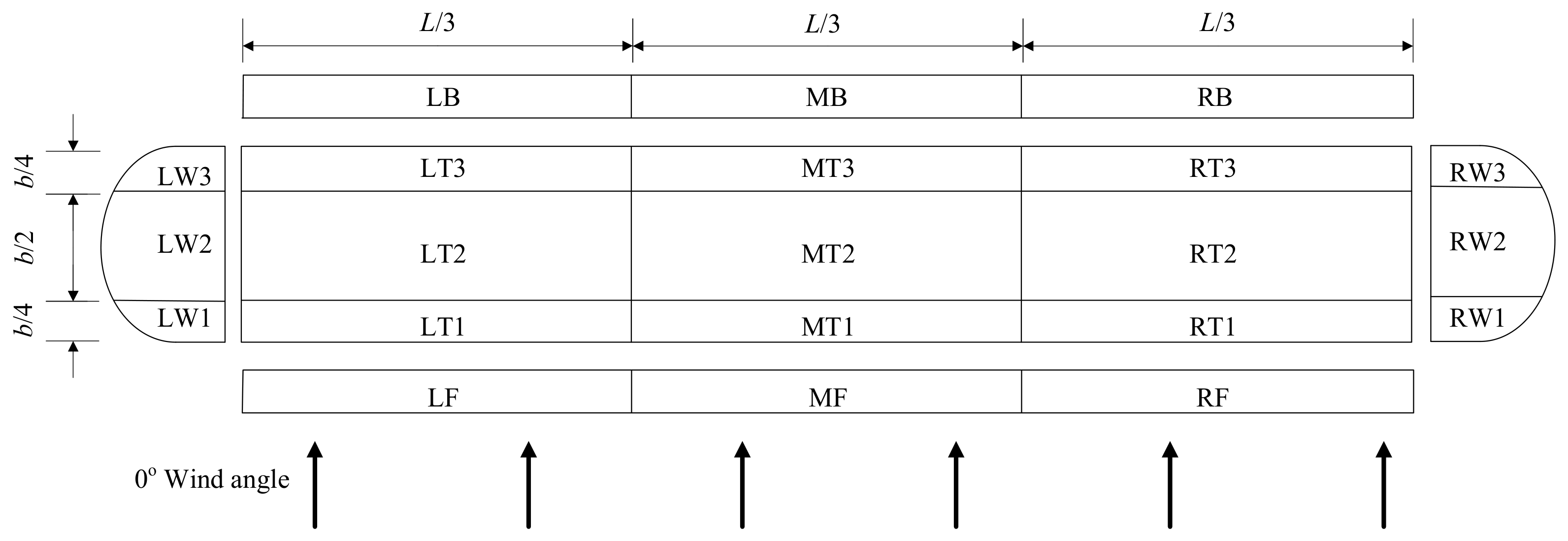
To evaluate spatial variations in wind pressure on the greenhouse surface, the greenhouse is partitioned into three equal segments along both the longitudinal and transverse directions, forming a grid of representative surface regions, based on the Code for the design load of horticultural greenhouse structures [28] and Standard for wind loads on roof structures in China [29]. This partitioning scheme allows calculation of local wind pressure coefficients for different structural surfaces. As illustrated in Figure 1, the windward wall is denoted as region F, and the leeward wall is denoted as region B. The roof surface is subdivided into three zones: T1, T2, and T3, corresponding respectively to the windward roof region, the central roof region, and the leeward roof region. The side surfaces perpendicular to the incoming flow are denoted as W. Additionally, the greenhouse is divided into left (L), middle (M), and right (R) sections along the span direction in order to capture potential asymmetric pressure distributions caused by flow interaction.

Figure 1. Wind pressure coefficient distribution zone of a plastic greenhouse [29].

3.2. Geometric Configuration of Greenhouse Clusters

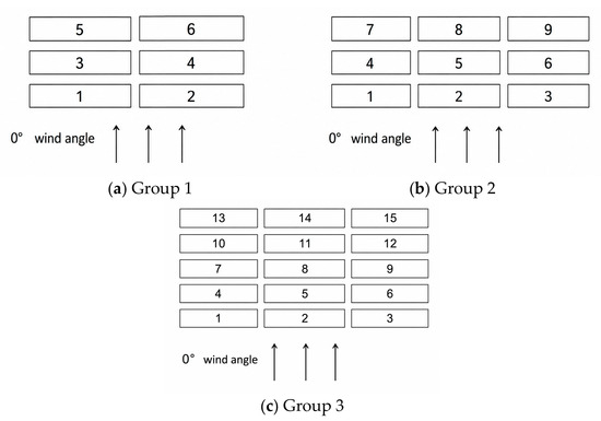
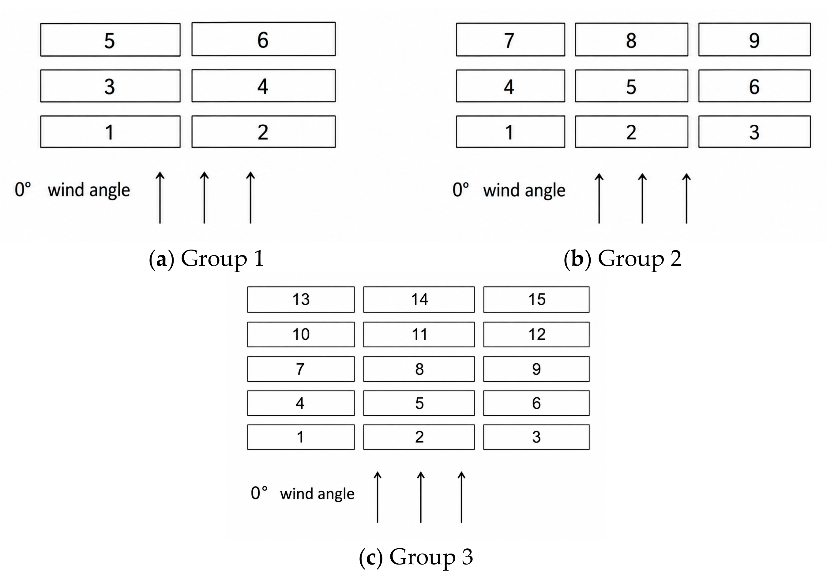
Field observations of greenhouse construction practices in Nyingchi, Tibet, indicate that plastic greenhouses are typically arranged in parallel rows to maximize land utilization while maintaining adequate solar radiation conditions [5]. Based on these practical considerations, three representative greenhouse cluster layouts are selected in this study: 2 × 3, 3 × 3, and 3 × 5, corresponding to Groups 1, 2, and 3, respectively.

In all configurations, the spacing between adjacent greenhouses in both longitudinal and transverse directions is set to 3 m. The geometric layouts and numbering scheme of the greenhouse clusters are shown in Figure 2. In the present study, only the 0° wind direction was considered, where 0° denotes wind approximately perpendicular to the longitudinal direction of the greenhouse cluster and to the greenhouse ridge direction. This wind direction was adopted as a representative unfavorable wind direction because previous CFD studies on greenhouse wind loads have shown that 0° wind-direction cases can produce large suction on windward roof regions and significant pressure variation on windward surfaces [25].

Figure 2. Layout diagram of plastic greenhouses.

It should be noted that the present study focuses on the influence of valley terrain and cluster arrangement under this representative unfavorable wind direction, rather than on the exhaustive identification of the critical wind direction among all possible wind angles.

4. Mountain Size and Wind Field Characteristics of the Valley

4.1. Selection of Valley Region

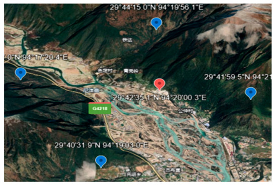
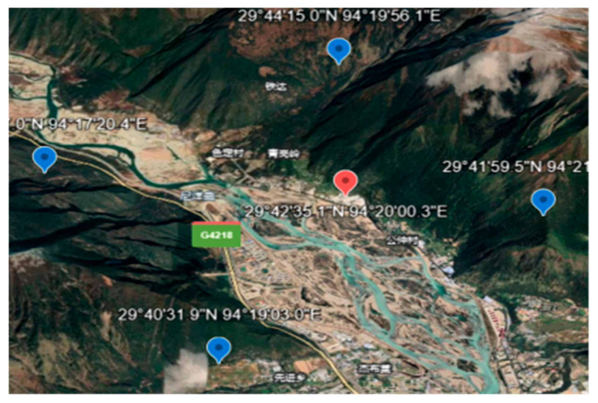
The Tibetan Plateau is characterized by complex mountainous terrain, where river valleys are mainly oriented along northeast–southwest and northwest–southeast directions. These terrain features significantly influence local wind characteristics near the ground surface, producing spatially non-uniform wind speed distributions and complex flow structures. Based on the distribution data of plastic greenhouses in Nyingchi, a representative valley region along the Nyang River was selected as the study area. As shown in Figure 3, the selected terrain domain covers an area of 7 km × 7 km and contains typical greenhouse construction areas within the valley-floor region.

Figure 3. Satellite map of the selected valley terrain domain and representative greenhouse cluster location marked by the red symbol (7 km × 7 km). Blue markers indicate surrounding meteorological stations, and the red marker indicates the representative greenhouse cluster location.

The dominant valley orientation in the selected area is northwest–southeast, and the prevailing wind direction is approximately aligned with the valley axis [30]. In this study, the terrain wind–field simulation was conducted under the 0° wind direction, which was defined as the direction approximately parallel to the northwest–southeast valley axis. The longitudinal axis of the greenhouse cluster was arranged perpendicular to the valley axis; therefore, the 0° terrain wind direction was also approximately normal to the greenhouse ridge direction and was consistent with the 0° wind direction adopted in the greenhouse cluster wind pressure simulation.

The red marker in Figure 3 indicates the representative location of the greenhouse cluster considered in this study, with an approximate geographic position of 29°42′35.1″ N, 94°20′00.3″ E. This location is situated on the relatively flat valley-floor area along the Nyang River and is bounded by mountain slopes on both sides, representing a typical siting condition for plastic greenhouse clusters in the Nyingchi valley region.

In the numerical simulation framework, this red-marked location was used as the reference position for linking the terrain wind–field simulation with the greenhouse wind pressure simulation.

4.2. Construction of Valley Terrain Model

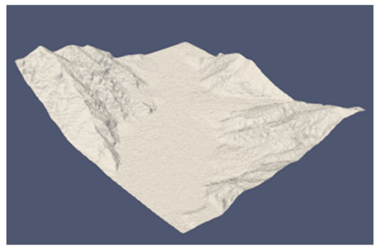
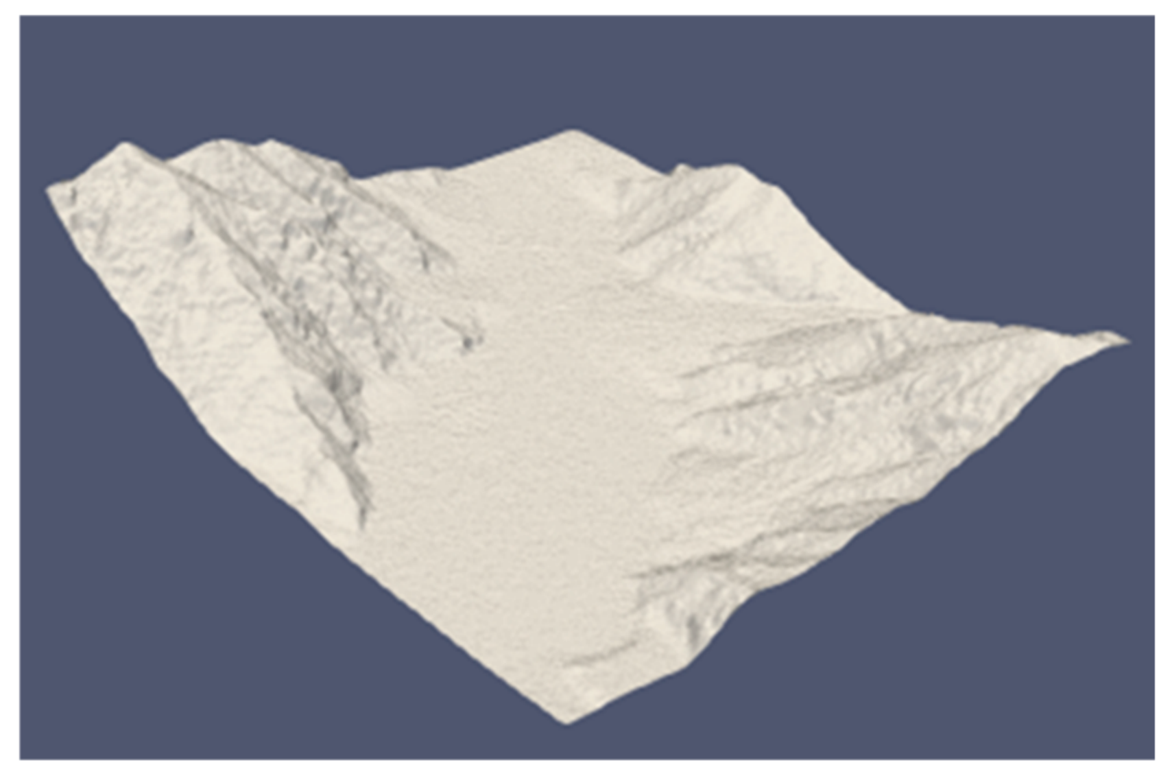
To accurately represent terrain-induced flow characteristics, a three-dimensional terrain model is constructed using digital elevation data. The digital elevation model (DEM) with a spatial resolution of 12.5 m is imported into ArcGIS10.8.2 software to extract contour elevation information for the selected region. After coordinate system transformation and data processing, the elevation data are exported and reconstructed into a three-dimensional terrain model using ParaView 5.10.1 software.

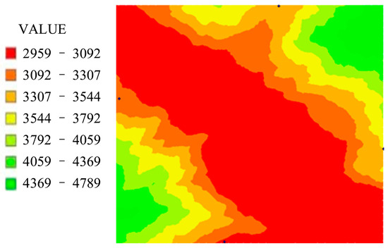
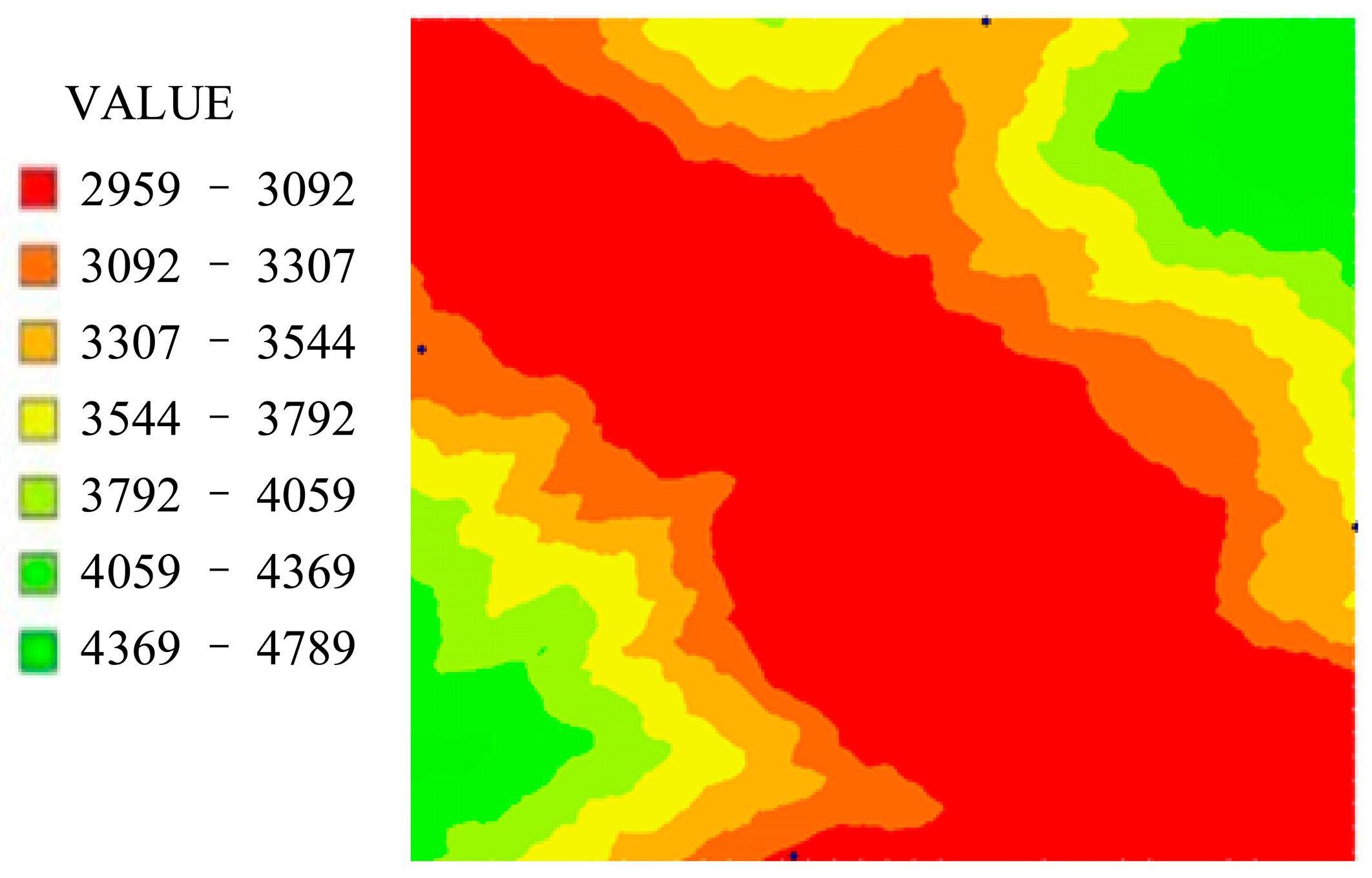
The reconstructed terrain model preserves the major geometric features of the valley, including mountain slopes and elevation variations, ensuring that the simulated wind field reflects realistic terrain-induced flow distortion. The elevation distribution of the selected region is shown in Figure 4, and Figure 5 illustrates the reconstructed three-dimensional terrain geometry.

Figure 4. Elevation map of the simulated area.

Figure 5. 3D Terrain Surface of the simulated area.

It should be noted that local obstacles such as nearby small buildings, vegetation, and other small-scale surface features were not explicitly modeled in the present terrain reconstruction; therefore, the simulations mainly capture the dominant topographic effects at the valley scale. Although these small-scale features were neglected, they may still influence the local wind field and wind pressure coefficient distribution, and their effects should be considered in future studies.

4.3. Air Properties Under High-Altitude Conditions

Air properties such as density and kinematic viscosity vary with altitude and influence the aerodynamic characteristics of the simulated flow field. Since the study area is located at an elevation of approximately 3000 m [31], air density is corrected according to atmospheric thermodynamic relationships [32]:

$$\rho ={\displaystyle \frac{p\times {10}^2}{RT}}\left(1-0.378{\displaystyle \frac{e}{p}}\right)$$

(1)

where T is the desired height temperature, K; R equal to 287.05; ρ is the density of the atmosphere at the reference elevation, kg/m³; p is the atmospheric pressure at the desired altitude, hPa; e is the water vapor pressure, hPa. The dew point temperature in Lhasa should be greater than −10.0 °C. The water vapor pressure is equal to the saturated water vapor pressure on the water surface, taken as 6.1075 hPa. Atmospheric pressure and altitude are closely related, and the formula for atmospheric pressure can be expressed as follows:

$$p=p_0\times {\left(1-{\displaystyle \frac{0.0065h}{288.15}}\right)}^{5.25588}$$

(2)

where p₀ is the standard atmospheric pressure, taken as 1013.25 hPa; h is the altitude of the desired altitude layer, m.

The dynamic viscosity $\mu$ of air is determined from the local air temperature using Sutherland’s law, and the kinematic viscosity is subsequently calculated as follows:

$$\nu ={\displaystyle \frac{\mu }{\rho }}$$

(3)

Based on an altitude of $h=3000$ m and an absolute air temperature of $T=280.15$ K, the atmospheric pressure, air density, and kinematic viscosity were calculated as 701.1 hPa, 0.997 kg/m³, and $1.76\times {10}^{-5}$ m²/s, respectively.

4.4. Numerical Simulation of Terrain-Induced Wind Field

4.4.1. Boundary Condition Settings and Transfer of Terrain-Induced Wind Field

The representative greenhouse location is situated on a relatively open valley-floor agricultural/suburban area with sparse low-rise obstacles; therefore, Terrain Category B was adopted according to GB 50009-2012 [31]. In GB 50009-2012, Terrain Category B represents suburban areas or small-to-medium-sized urban areas with relatively sparse low-rise buildings. The inlet boundary condition was defined using a vertically varying exponential wind speed profile to represent atmospheric boundary-layer characteristics over terrain with surface roughness corresponding to Class B terrain conditions [31]. The inlet boundary condition was defined using a vertically varying exponential wind speed profile corresponding to Terrain Category B according to GB 50009–2012 [31]. Because the present study focuses on normalized mean wind pressure coefficients rather than dimensional pressures or forces, the basic wind speed was used directly as the reference velocity at a height of 10 m. Based on the basic wind pressure with a 10-year return period, the wind speed is calculated as 31.64 m/s for the 3 s averaging interval [33]. The same reference velocity and inlet-profile definition were applied consistently to all simulated cases. Therefore, the selected velocity magnitude does not affect the comparative conclusions based on $C_p$. The inlet velocity profile was expressed as $V_z=V_0{\left({\displaystyle \frac{Z}{10}}\right)}^{0.16}$, where $V_0$ is the basic reference wind speed at a height of 10 m, and $z$ is the height above the ground surface. The inlet turbulence quantities were specified using the standard atmospheric boundary-layer formulation in Fluent, with turbulence intensity and turbulent kinetic energy profiles calculated consistently with the inlet velocity profile.

For the terrain-scale simulation, the exponential wind profile was imposed at the upstream boundary of the full valley terrain domain. The outlet boundary was set as a pressure outlet. The ground surface was treated as a no-slip wall, while the lateral and top boundaries were specified to minimize their influence on the near-ground flow field. The 0° wind direction was defined as the direction approximately parallel to the northwest–southeast valley axis, which corresponds to the prevailing wind direction in the selected valley region.

To link the terrain-scale wind–field simulation with the greenhouse-scale wind pressure simulation, a one-way transfer strategy was adopted. The 7 km × 7 km terrain simulation was first conducted without explicitly including the greenhouse structures. After convergence, wind speed data near the representative greenhouse location marked in Figure 3 were extracted from the terrain-scale result and fitted to define a terrain-modified vertical inlet velocity profile. This fitted profile was subsequently prescribed at the inlet of the reduced greenhouse-scale valley terrain model. The full three-dimensional terrain flow field was not directly mapped onto the greenhouse-scale inlet, and the greenhouse structures did not feed back into the terrain-scale flow field. Therefore, the adopted procedure represents a one-way profile-transfer approach rather than a fully coupled multiscale simulation.

It should be noted that the present simulations were conducted using a steady RANS framework. Therefore, the numerical results mainly represent time-averaged wind–field and mean pressure coefficient characteristics. Unsteady vortex shedding, transient separation, and peak pressure fluctuations in complex terrain cannot be fully resolved by the present method. The results should therefore be interpreted as comparative mean-flow predictions, and the limitations of the RANS approach are further discussed in Section 6.2.

For the plain-terrain reference case, the original exponential atmospheric boundary-layer wind profile was directly imposed at the inlet of the greenhouse-scale computational domain. For the valley terrain case, the same upstream exponential profile was first imposed at the inlet of the full valley terrain domain, and the terrain-modified local wind condition obtained at the representative greenhouse location was then used to adjust the inlet condition of the greenhouse-scale valley case. Therefore, the difference between the plain terrain and valley terrain greenhouse simulations was introduced through the local inlet wind condition informed by the terrain-scale simulation, while the greenhouse geometry, layout, mesh strategy, wall boundary conditions, turbulence model, and numerical settings were kept consistent.

It should be noted that this procedure is a one-way transfer approach rather than a fully coupled multiscale simulation. The greenhouse structures were not included in the terrain-scale simulation and did not feed back into the large-scale valley wind field. In addition, the full three-dimensional terrain flow field was not directly mapped onto the greenhouse-scale inlet. The complex terrain effect was introduced through the terrain-modified local wind condition at the representative greenhouse site, which was subsequently used as the inlet condition for the valley terrain greenhouse-scale simulation.

4.4.2. Turbulence Model Validation

To evaluate the suitability of the turbulence model for predicting mean surface wind pressure coefficients, six commonly used RANS turbulence models were compared, including the standard k-ε model, realizable k-ε model, renormalization group (RNG) k-ε model, standard k-ω model, shear stress transport (SST) k-ω model, and baseline (BSL) k-ω model.

It should be clarified that the validation case was not a plastic greenhouse cluster or a valley terrain model. Instead, a benchmark case of airflow around a surface-mounted cubic building was adopted. This benchmark was selected because it provides well-documented mean surface pressure coefficient data under atmospheric-boundary-layer flow conditions and has been widely used for evaluating turbulence models in computational wind engineering. Therefore, the purpose of this validation was to compare the relative performance of different RANS models in predicting mean pressure coefficients around a low-rise bluff body, rather than to provide a direct geometry-specific validation for arched greenhouses in valley terrain.

Comparative validation was performed using benchmark mean surface pressure coefficient data for airflow around a surface-mounted cube. The wind-tunnel data refer to the data reported by Murakami and Mochida [34], whereas the full-scale field data were taken from Richards and Hoxey [35]. These two datasets were used as reference pressure coefficient datasets for comparison with a single cubic-building CFD validation model, rather than as two separately reconstructed CFD inflow cases.

The wind-tunnel data should not be interpreted as a simulation or scaled reproduction of the full-scale field experiment. Accordingly, the inflow settings summarized in Table 1 apply only to the present cubic-building CFD validation simulation. The full-scale field data were used in their published normalized form, based on the reference dynamic pressure measured in the original field study, and were not used to define the inlet turbulence conditions of the present CFD model.

Table 1. CFD settings for the cubic-building benchmark validation simulation.

Item	Setting Used in Validation	Source/Explanation
Computational domain for validation	21H × 11H × 6H	Present validation simulation setting; H denotes the cube side length. The resulting blockage ratio is approximately 1.52%, below 3%.
Benchmark geometry	Surface-mounted cubic building; cube side length H = 0.2 m	Present validation simulation setting.
Mesh size/elements	1,045,183 elements	Solver setting
Inlet mean velocity profile	Exponential wind profile: $V_z=V_0{\left({\displaystyle \frac{Z}{Z_0}}\right)}^{0.16}$, $Z_0$ = 10 m	Adopted to reproduce the incoming boundary-layer flow used in the benchmark case [34].
Reynolds number	Re = ${\displaystyle \frac{uH}{v}}$ = 7 × 104	The value corresponds to the wind-tunnel-scale cube model with H = 0.2 m; it is not the Reynolds number of the full-scale field case or the final greenhouse simulations.
Inlet turbulence quantities	Turbulence intensity: I = 0.16 Re−1/8 Inlet turbulent kinetic energy: $k(z)=\frac{3}{2}{\left(V_z\cdot I\right)}^2$ Turbulent kinetic energy dissipation rate: $\epsilon \left(z\right)=C_{\mu }k{\left(z\right)}^{3/2}/l$, $l$ is the turbulence integral scale, $C_{\mu }$ = 0.09 Specific dissipation rate: $\omega (z)={\displaystyle \frac{\epsilon \left(z\right)}{C_{\mu }k\left(z\right)}}$	Solver inlet formulations; not independent experimental quantities.
Outlet boundary conditions	Pressure-outlet	Standard outflow boundary condition for the validation domain.
Ground and cube surfaces	No-slip wall	Physical wall boundary condition.
Top and lateral boundaries	Symmetry boundary condition	Used to reduce artificial shear effects at domain boundaries.
Pressure–velocity coupling	Coupled algorithm	Numerical solution scheme; not a physical boundary condition.
Near-wall treatment	standard wall functions	Solver setting
Spatial discretization	Second-order upwind scheme	Solver setting
Momentum equation convergence criterion	Residuals below 1 × 10−4 and monitored surface pressure coefficients reaching stable values	Solver setting

The CFD settings used for the cubic-building benchmark validation are summarized in Table 1. Table 1 applies only to the turbulence model validation case for the surface-mounted cube and does not apply to the subsequent terrain-scale or greenhouse-scale simulations, whose boundary conditions and mesh settings are described separately in Section 4.4.1 and Section 5.1. In this validation case, the prescribed inlet velocity profile and turbulence quantities were implemented in Fluent through a User-Defined Function (UDF).

In Table 1, H denotes the side length of the cubic benchmark model. The computational domain used in the present validation simulation was 21H × 11H × 6H, giving a blockage ratio of approximately 1.52%, below the commonly recommended limit of 3% for external-flow simulations.

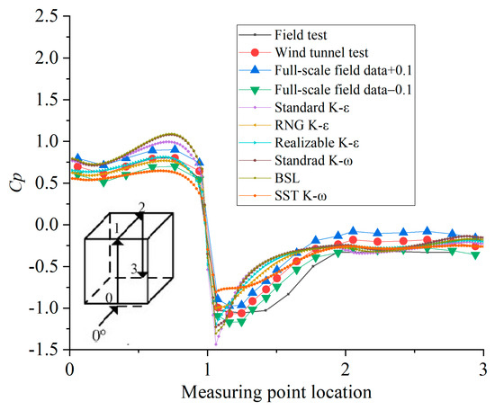
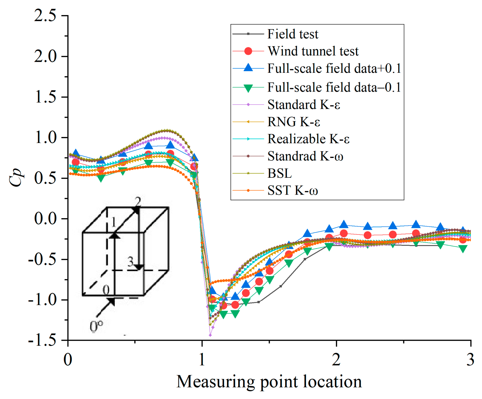
As the model’s measured data were published in Ref. [35], a comparison of the field test, wind tunnel results, and simulation results from the six turbulence models is achieved and shown in Table 2. Figure 6 compares the mean surface pressure coefficients predicted by different RANS turbulence models for the cubic-building validation model with two independent reference datasets: the wind-tunnel data reported by Murakami and Mochida [34] and the full-scale field data reported by Richards and Hoxey [35]. The comparison path follows the vertical centerline of the cubic model, extending from the base of the windward face (Point 0) to the top edge (Point 1), across the roof surface (Points 1–2), and down to the base of the leeward face (Point 3), consistent with the pressure-tap arrangement reported by Richards and Hoxey [35].

Table 2. Mean absolute errors of surface wind pressure coefficients for different models based on 20 comparison points along the vertical centreline path from Point 0 to Point 3 shown in Figure 6.

Error	Standard k-ε	RNG k-ε	Realizable k-ε	Standard k-ω	BSL	SST k-ω
Errors with the field test	0.242	0.207	0.196	0.240	0.245	0.204
Errors with the wind tunnel test	0.204	0.149	0.144	0.182	0.198	0.177

Figure 6. Comparison of simulated mean wind pressure coefficients with benchmark data for a surface-mounted cubic building.

As shown in Table 2, the RNG k-ε and realizable k-ε models produced comparable mean absolute errors. The realizable k-ε model gave the lowest error among the six models for both the wind-tunnel and full-scale reference datasets, but the difference from the RNG k-ε model was small. Therefore, the realizable k-ε model was selected as a representative RANS model for the subsequent greenhouse simulations, while this selection should not be interpreted as a statistically definitive superiority over the RNG k-ε model.

The reference data used for validation were obtained from two sources: the wind-tunnel benchmark data reported by Murakami and Mochida [34] and the full-scale field measurement data reported by Richards and Hoxey [35]. The mean absolute error in Table 2 was calculated using 20 pressure coefficient comparison points extracted along the vertical centreline path shown in Figure 6. In the comparison, the following equation of error is:

$$error=\sqrt{{\displaystyle \frac{1}{n}}{\displaystyle \sum _{i=1}^n{\left({\mathrm{Value}}_{i,\mathrm{Test}}-{\mathrm{Value}}_{i,\mathrm{Turbulence}\text{-}\mathrm{model}}\right)}^2}}$$

(4)

It should be noted that the full-scale field measurement data contain greater uncertainty than wind-tunnel data because natural wind speed, wind direction, turbulence characteristics, and reference dynamic pressure cannot be exactly reproduced. Richards and Hoxey [35] reported that approximately 90% of the normalized data for mean pressure coefficients lie within a band of ±0.1. Therefore, the full-scale data were used mainly for evaluating the overall trend of the predicted mean pressure coefficients rather than for exact pointwise calibration.

It should also be noted that the benchmark validation case adopted in this study is not geometrically identical to the arched plastic greenhouse investigated in the subsequent simulations. The cubic building has sharp edges and strong corner-induced flow separation, whereas the arched greenhouse roof has a smoother curved surface and different flow separation and reattachment characteristics. Therefore, the validation should be understood as an assessment of the ability of the turbulence models to predict mean surface pressure coefficients for low-rise bluff-body flows under atmospheric boundary-layer conditions, rather than as a direct geometry-specific validation for arched greenhouses.

The realizable k-ε model was selected because it produced the smallest overall error in the benchmark comparison of mean pressure coefficients and has been commonly used in CFD simulations of wind pressure around low-rise buildings and greenhouse structures. Compared with the standard k-ε model, the realizable formulation improves the representation of strain-rate effects and separated flows, which is relevant for the prediction of mean pressure distribution around curved-roof greenhouse structures. However, the cubic-building benchmark does not fully reproduce the aerodynamic characteristics of arched plastic greenhouse clusters in valley terrain. The validation results should therefore be interpreted as support for the comparative prediction of mean surface pressure coefficients using the selected RANS model, rather than as a complete validation of all unsteady aerodynamic features of greenhouse clusters under complex terrain conditions. Since the present study focuses on the comparative influence of valley terrain and cluster arrangement on mean wind pressure coefficients and wind load shape factors, the realizable k-ε model was considered appropriate for the mean-flow comparative analysis conducted in this work.

4.4.3. Computational Domain and Mesh Independence Validation

For an isolated building or obstacle, computational-domain adequacy is commonly assessed using a frontal-area blockage ratio. However, the present terrain represents a continuous mountainous lower boundary rather than an isolated obstacle, and a conventional building-type blockage ratio cannot be determined unambiguously from the available terrain model. Therefore, the upper-boundary height was selected using a pragmatic sensitivity-based approach. Previous domain-height testing [36] showed that, when the upper boundary was located 3000 m above the reference level, further increases in domain height produced negligible changes in the wind field within the lower 600 m, which contains the region of interest for the greenhouse simulations.

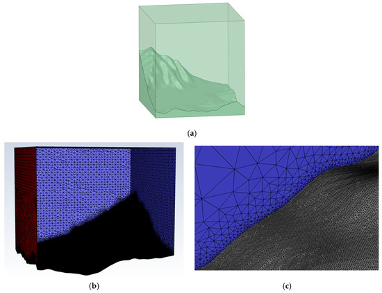
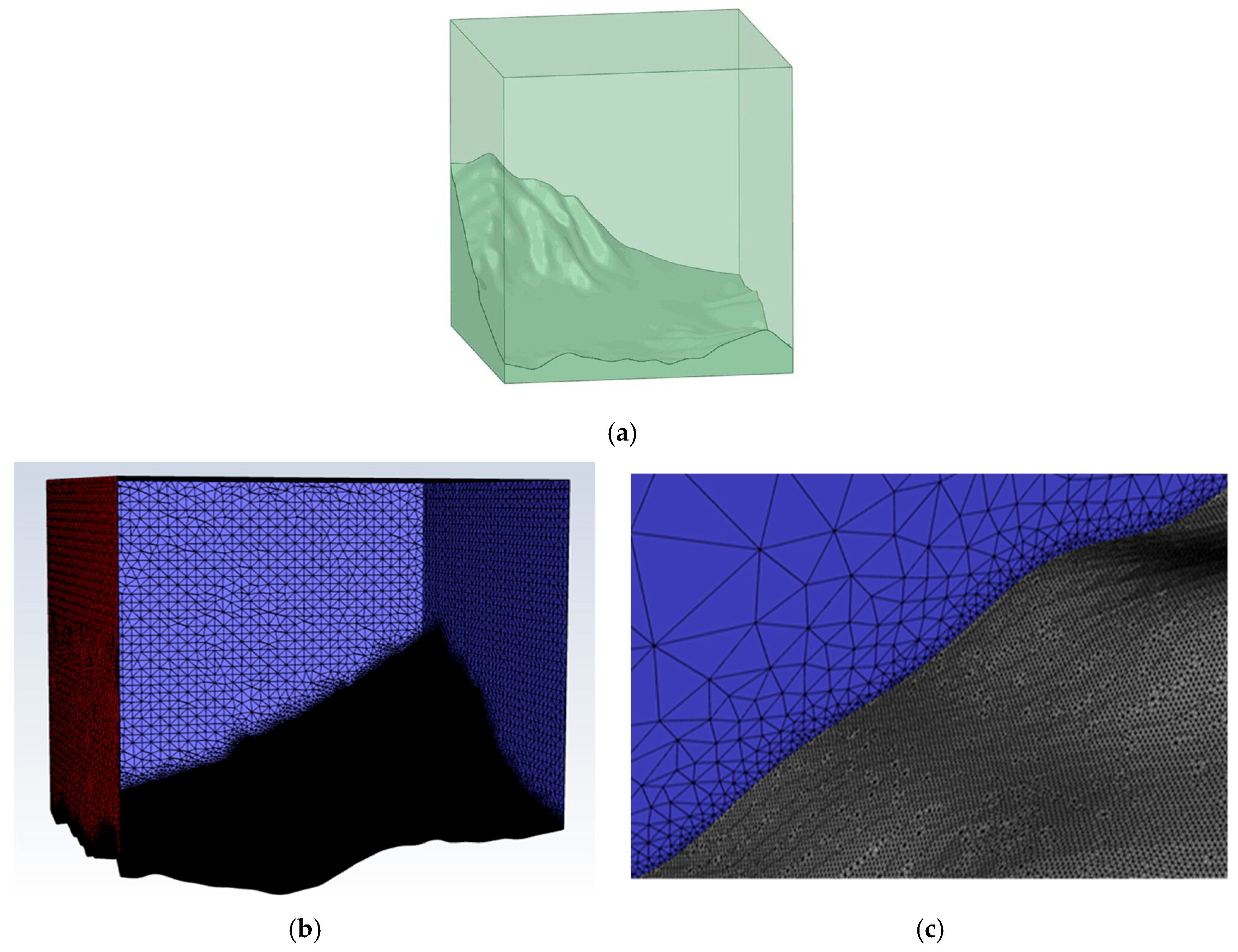
Mesh independence verification is conducted to evaluate the influence of mesh resolution on simulation accuracy. Five maximum mesh sizes (10 m, 20 m, 30 m, 40 m, and 50 m) are tested under identical boundary conditions. A refined mesh region is generated near the terrain surface, with a first-layer boundary layer thickness of 1 m, a mesh growth rate of 1.1, and a maximum mesh size of 20 m. The global maximum wind velocity on the mountain surface obtained within the entire computational domain under different maximum mesh sizes is selected as the target monitoring parameter to evaluate grid convergence. The computational fluid domain and boundary layer mesh of the mountain model are shown in Figure 7.

Figure 7. Computational domain and mesh generation for the mountain terrain model. (a) Computational fluid domain; (b) Schematic diagram of the mesh generation for the mountain model; (c) Schematic diagram of the boundary layer mesh for the mountain model.

As can be seen from Table 3, across the five different maximum mesh sizes tested, the deviations in the simulated maximum wind velocity on the mountain surface are minimal when compared to the 20 m mesh size, with a maximum error of only 1%. Considering computational accuracy and efficiency, a maximum mesh size of 20 m is selected for terrain simulation.

Table 3. Simulation results under different maximum mesh sizes of mountain surface.

Maximum Mesh Size (m)	Minimum Mesh Quality	Number of Elements (104)	Error (Relative to 20 m)
10 m	0.37	10,840	1%
20 m	0.35	7862	0
30 m	0.33	5534	0.1%
40 m	0.31	4138	0.1%
50 m	0.28	2094	0.7%

5. Research and Analysis on the Shape Factor of the Wind Load

The terrain-scale simulation was used to determine the terrain-modified inflow condition at the representative greenhouse location identified in Figure 3. The same undisturbed power-law atmospheric-boundary-layer profile was prescribed at the inlet of the terrain-scale valley simulation and was also used directly for the plain-terrain greenhouse simulations. In the valley terrain case, the airflow was modified by the surrounding terrain before reaching the representative greenhouse location. Wind speed data extracted near this location were fitted to define the inlet condition of the reduced greenhouse-scale valley model. The full three-dimensional terrain flow field was not directly mapped onto the greenhouse-scale domain. Therefore, the differences between the plain terrain and valley terrain greenhouse simulations arise from the terrain-modified inflow condition rather than from different prescribed upstream atmospheric-boundary-layer profiles.

5.1. Meshing and Boundary Conditions of Greenhouse Clusters

Before constructing the greenhouse-scale computational domains, the relationship between the terrain-scale and greenhouse-scale simulations was clarified. The smaller greenhouse-scale domains did not include the full 7 km × 7 km valley terrain. Instead, the influence of the complex terrain was introduced through the terrain-modified local wind condition obtained at the representative greenhouse cluster location from the terrain-scale simulation. In the plain-terrain reference case, the inlet condition of the greenhouse-scale domain was defined using the undisturbed exponential atmospheric boundary-layer wind profile. In the valley terrain case, the inlet condition was adjusted according to the local wind condition obtained from the terrain-scale simulation at the representative greenhouse site. Thus, the comparison between the plain terrain and valley terrain greenhouse simulations reflects the influence of the terrain-modified incoming wind condition, rather than a fully coupled simulation in which the greenhouse structures are resolved inside the complete valley domain.

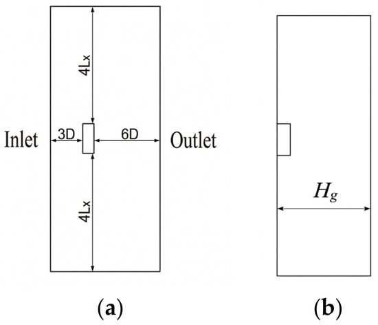
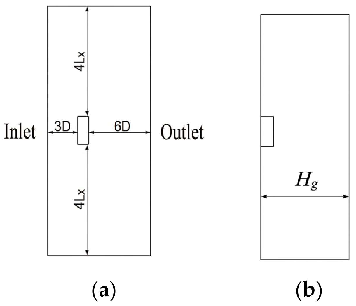
The blockage ratio of the computational domain for plastic greenhouses should not exceed 3%. For numerical simulation of this group of greenhouses, the dimensions of the flow field domain are as follows: length parallel to the incoming flow ≥ 10D, length perpendicular to the incoming flow ≥ 9L_x, and height ≥ 5H_G, where D is the width of the cluster parallel to the incoming flow, m, L_x is the length of the cluster, m, and H_G is the height of the greenhouse. As shown in Figure 8, the computational domain size of the greenhouse cluster is set as follows: 9L_x in the length direction, 10D in the width direction, and H_g = 100 m in the height direction. The size of each greenhouse group is shown in Table 4.

Figure 8. Calculation field size of plastic greenhouses. (a) Horizontal dimension of the computational domain. (b) Vertical dimension of the computational domain.

Table 4. Size table of greenhouse groups.

Parameters	Group 1	Group 2	Group 3
D/m	27	27	47
Lx/m	91	138	138
Fluid domain width/m	270	270	470
Fluid domain length/m	819	1242	1242
Fluid domain height/m	100	100	100

The plastic greenhouse group model is placed at the 1/3 position in front of the windward side of the computational domain. This arrangement provides ample pre-development distance for the incoming flow, ensuring sufficient development of the inlet flow field while effectively avoiding interference from wall expansion effects on the calculation results. The greenhouse cluster geometries were constructed using UG NX 12.0 software and exported as Parasolid files. The meshes were generated using Ansys ICEM CFD 2022 R1 software, with a maximum mesh size of 20 m in the outer computational domain and refined meshes near the greenhouse surfaces. To improve the resolution of the near-surface pressure field, local mesh refinement was applied on the greenhouse surfaces, with the mesh size in the refined region set to 0.1 m. Five refinement layers were used near the greenhouse surfaces, and the boundary-layer growth rate was set to 1.3. The total number of cells for the three greenhouse cluster models was approximately 1.35 million, 1.86 million, and 3.15 million, respectively.

For each greenhouse-scale simulation, a velocity inlet and a pressure outlet were assigned according to the corresponding terrain condition. For the plain-terrain cases, the inlet followed the original undisturbed power-law atmospheric-boundary-layer profile. For the valley terrain cases, wind speed data extracted near the representative greenhouse location from the 7 km × 7 km terrain-scale simulation were fitted to define a terrain-modified vertical velocity profile, which was then prescribed at the greenhouse-scale inlet. The full three-dimensional terrain flow field was not directly mapped onto the reduced domain. The greenhouse surfaces were defined as no-slip wall boundaries, while the top and lateral boundaries of the computational domain were treated as symmetry boundaries to reduce their influence on the flow around the greenhouse cluster.

The mesh-quality indicators, including Jacobian, aspect ratio, and skewness, were checked before calculation. No negative-volume cells were observed, and the mesh quality satisfied the basic requirements for Fluent simulations. These checks ensured the geometric validity and numerical stability of the generated meshes. The numerical solution settings that could be verified from the original simulation records are summarized in Table 5.

Table 5. Verified numerical solution settings for the greenhouse-scale wind pressure simulations.

Parameter	Setting Result
Solver	Steady-state solution
Turbulence model	Realizable k-ε
Pressure–velocity coupling	SIMPLEC
Pressure discretization	Second-order
Momentum discretization	Second-order upwind
Turbulence equations discretization	Second-order upwind
Near-wall treatment	Standard wall functions
Momentum equation convergence criterion	10−6
Convergence criteria for the continuity equation and k-ε equations	10−3

5.2. Definition of Wind Pressure Coefficient

Wind pressure acting on greenhouse surfaces is influenced by incoming wind characteristics, structural geometry, and aerodynamic interaction between adjacent structures. In wind engineering practice, the wind pressure coefficient is commonly used to describe the relationship between local surface pressure and reference dynamic pressure of the incoming flow. The wind pressure coefficient is defined as follows:

$$C_{pi}={\displaystyle \frac{P_i-P}{0.5\rho V_{10}^2}}$$

(5)

where C_pi is the wind pressure coefficient at surface point i; P_i is the local static pressure at point I, Pa; $P$ is the static pressure at the inlet boundary of the corresponding greenhouse-scale computational domain, Pa; $\rho$ is the air density, kg/m³; $V_{10}$ is the velocity obtained from the prescribed inlet profile at 10 m above the local ground surface, m/s. For the single-greenhouse and plain-terrain array cases, V₁₀ was obtained from the original undisturbed power-law profile. For the valley terrain array cases, V₁₀ was obtained from the fitted terrain-modified inlet profile. The same reference definition was applied to Groups 1, 2, and 3. The corresponding P and V₁₀ values for each simulation were used consistently to normalize the simulated surface pressures.

Positive values of C_p indicate compression relative to the reference pressure, whereas negative C_p values indicate suction. For the arched greenhouse roof, negative C_p indicates suction and may result from local flow acceleration over the curved surface, as well as from flow separation or vortex formation.

The wind load shape factor was determined from the area-weighted mean wind pressure coefficient over the corresponding surface region. Since the pressure coefficient defined in Equation (5) was normalized using the 10 m reference dynamic pressure, the resulting shape factor represents the aerodynamic shape effect of the greenhouse surface without including the wind pressure height variation coefficient, as shown in Equation (6):

$${\mu }_s={\displaystyle \frac{{\displaystyle \sum _i{C}_{pi}{A}_i}}{A}}$$

(6)

where ${\mu }_s$ is the wind load shape factor; $C_{pi}$ is the wind pressure coefficient value at the ith representative point of the partition; A_i is the surface area represented by the ith point, m²; A is the total area of the calculated surface, m².

The terrain correction coefficients were calculated as case-specific indicators to quantify the relative difference between the selected valley terrain case and the corresponding plain-terrain reference case. Because these coefficients depend on the selected terrain, greenhouse layout, wind direction, and numerical settings, their detailed definitions and values are provided in Equation (A1) of Appendix A rather than being presented as generally applicable design coefficients.

5.3. Wind Pressure Coefficient Distribution for Plain Terrain

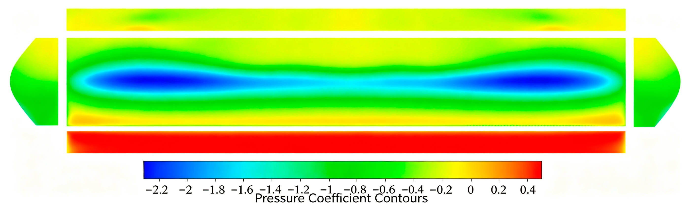
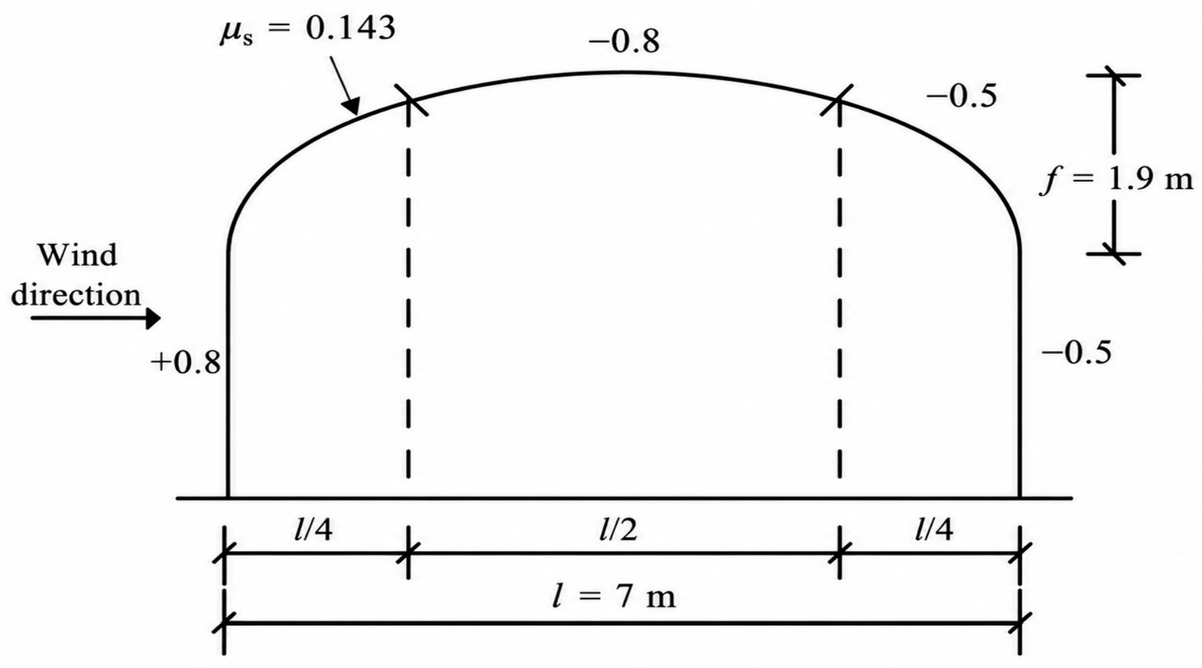
The pressure coefficient contours on a single greenhouse under plain-terrain conditions are simulated and shown in Figure 9. The wind load shape factors at different regions of the single greenhouse were specified according to the flat-terrain design code. For the windward roof, the corresponding shape factor was obtained by linear interpolation based on the code-specified values. The resulting shape factors are shown in Figure 10.

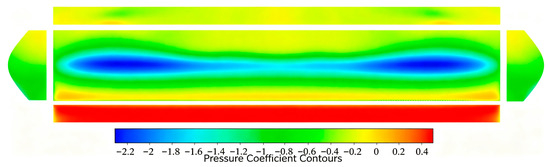
Figure 9. Pressure coefficient contours on the surface of a single plastic greenhouse under the 0° wind direction. Note: The color scale in this figure is independent of those used in the subsequent figures; therefore, colors should not be compared directly across figures.

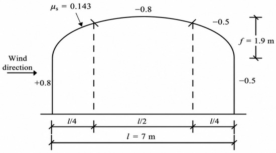
Figure 10. Pressure coefficient zones and reference coefficients for the single-greenhouse code comparison [28].

To provide a reference for the subsequent greenhouse-array analysis, the single-greenhouse CFD result was compared with the pressure coefficients/shape factors specified in the relevant design code [28]. Since Figure 9 presents pointwise C_p contours, the CFD values were area-averaged over the corresponding roof and wall zones before comparison with the code coefficients. This comparison was used only as a baseline check for the single-greenhouse simulation and not as a direct validation of the greenhouse-array results.

5.4. Analysis of the Simulation Results of Group 1 (2 × 3 Arrangement)

5.4.1. Pressure Coefficient Contours on Group 1 in a Valley Area

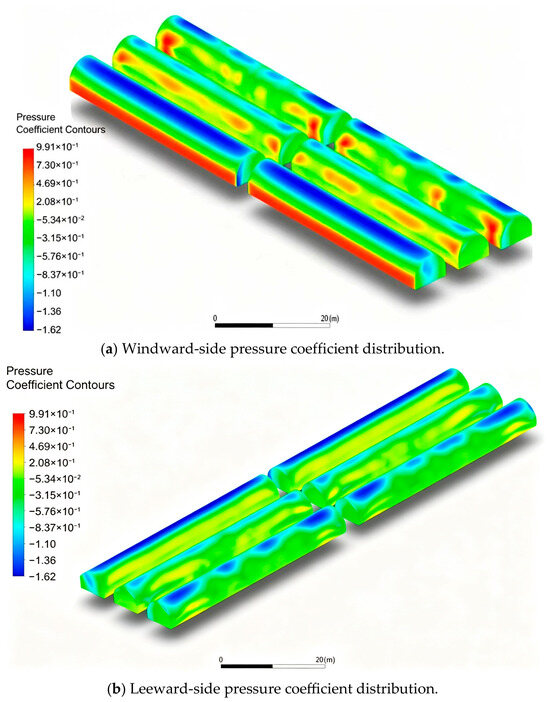
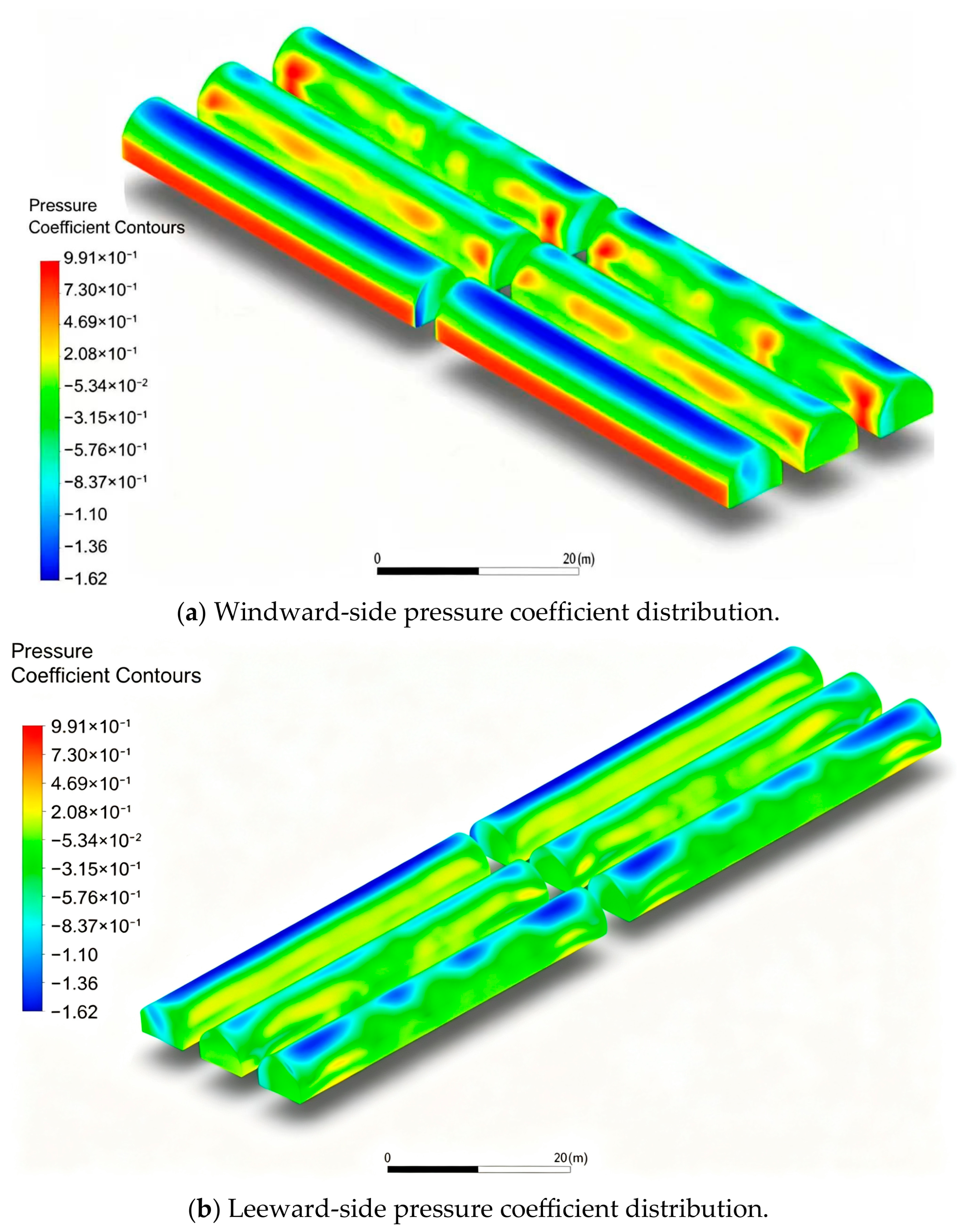
The wind pressure coefficient distribution of the 2 × 3 greenhouse cluster under valley terrain conditions is illustrated in Figure 11. The results show that the spatial distribution of surface wind pressure is strongly influenced by the combined effects of terrain-induced flow distortion and aerodynamic interference between adjacent greenhouses.

Figure 11. Wind pressure coefficient contours of Group 1 under the 0° wind direction. Note: To make the influence of complex terrain clearer, the corresponding plain-terrain numerical results are provided through the C_p tables and discussion, rather than being plotted as separate contour panels. A consistent C_p color scale is used within each individual comparison in the subsequent tablesables to avoid misleading interpretation based only on color intensity.

5.4.2. Comparison of C_p on Group 1 in Valley Areas and Plain Terrains

The ratios listed in Table 6 are CFD-based relative indicators calculated from the predicted pressure coefficients. The reference values were taken from the single-greenhouse flat-terrain case shown in Figure 9. Therefore, these ratios should not be interpreted as experimentally validated correction factors or as design-code coefficients. They provide only a case-specific comparison between the simulated greenhouse-array cases and the single-greenhouse flat-terrain reference. Because no corresponding reference data are available for the greenhouse arrays themselves, the comparison is not a strictly like-for-like comparison and should be interpreted with caution.

Table 6. Ratios of the C_p between valley topography and the plain region.

Shed Number	LF	MF	RF	LB	MB	RB	LW1	LW2	LW3	RW1	RW2	RW3	LT3	MT3	RT3	LT2	MT2	RT2	LT1	MT1	RT1
1	0.805	0.804	0.800	1.652	0.812	0.779	0.521	1.493	0.647	0.868	0.933	6.963	0.520	0.755	0.621	0.790	0.783	0.803	0.803	0.779	0.795
2	0.799	0.802	0.801	0.632	0.759	1.970	0.860	0.948	4.230	0.737	1.573	0.383	0.573	0.579	0.317	0.810	0.794	0.780	0.800	0.787	0.803
3	1.106	0.919	0.678	4.175	0.203	0.302	0.361	0.497	1.589	0.648	0.716	0.444	0.802	0.158	0.501	0.812	0.677	0.785	0.763	0.724	0.704
4	0.511	0.803	1.038	0.616	0.037	0.002	0.605	0.677	0.325	0.334	0.606	1.810	0.317	0.555	1.441	0.782	0.702	0.822	0.684	0.866	0.656
5	0.734	0.164	0.648	1.907	1.189	0.878	0.767	0.681	1.243	0.805	0.802	0.815	0.958	0.862	1.020	0.835	0.726	0.817	2.031	0.236	1.297
6	0.449	0.265	0.642	0.644	2.149	0.158	0.665	0.846	0.756	0.898	0.631	1.051	0.845	0.643	0.733	0.824	0.700	0.896	1.142	0.090	1.298

Note: The $C_p$ ratio is defined as $C_{p,\mathrm{v}\mathrm{a}\mathrm{l}\mathrm{l}\mathrm{e}\mathrm{y}}/C_{p,\mathrm{p}\mathrm{l}\mathrm{a}\mathrm{i}\mathrm{n}}$. When $C_{p,\mathrm{p}\mathrm{l}\mathrm{a}\mathrm{i}\mathrm{n}}$ is close to zero, the ratio becomes numerically sensitive and should be interpreted together with the corresponding original $C_p$ values. Large or negative ratios do not necessarily indicate proportional amplification or reduction in the physical wind pressure; further discussion is provided in Section 5.7.

As shown in Table 6, the aerodynamic behavior of the 2 × 3 greenhouse layout indicates that the first-row greenhouses dominate the windward load response due to their direct exposure to the incoming flow. The significantly larger pressure coefficients observed on Sheds No. 1 and No. 2 result from stagnation effects generated by frontal wind impingement.

5.4.3. Calculation of the Shape Factor of the Wind Load

The shape factors of wind load for Group 1 are summarized in Table 7, and the corresponding correction coefficients relative to the Chinese Load Code are presented in Table A1 of Appendix B. The design-code coefficients listed in Table 7 refer to an isolated single greenhouse under level-terrain conditions. They are used here only as baseline references for the single-greenhouse CFD result and should not be interpreted as code values for greenhouse arrays or complex terrain conditions.

Table 7. Shape factor of the wind load of Group 1 in valley topography.

Shed Number	F	B	T1	T2	T3
1	0.722	0.114	−0.541	−1.226	0.300
2	0.720	0.107	−0.542	−1.229	0.290
3	0.117	0.090	0.170	−0.650	−0.450
4	0.094	0.010	0.171	−0.658	−0.380
5	0.092	−0.269	0.068	−0.853	−0.361
6	0.086	−0.410	0.066	−0.860	−0.348
Chinese Code GB/T 51183-2016 [28]	0.800	−0.500	0.143	−0.800	−0.500
USA NGMA 2004 [37]	0.800	−0.500	0.106	−0.971	−0.500
EU EN 13031-1:2019 [38]	0.600	−0.300	0.300	−1.000	−0.400
Korea MAFRA 1999 [39]	0.800	−0.400	−0.600	−0.7–−0.5	−0.200

As shown in Table 7, under 0° wind direction, a prominent high positive pressure zone is concentrated on the windward wall (Zone F) of the leading greenhouse (Shed 1). This indicates that the oncoming airflow decelerates upon frontal impingement and forms a stagnation region, which generally corresponds to the macro-trends found in major statutory specifications such as Chinese GB/T 51183 [28] (+0.8), European EN 13031-1 [38] (+0.6), and Korean MAFRA [39] (+0.8). As the flow passes from the windward wall to the roof sectors, the CFD results show spatial variations in the roof pressure coefficients across Zones T1, T2, and T3. These variations reflect the combined influence of greenhouse-array interference and the terrain-modified incoming flow.

The comparison between Table 7 and Figure 10 shows that the CFD result captures the same general pressure pattern as the design codes, namely positive pressure on the windward wall and suction over the roof. However, the local extrema in Figure 10 should not be compared directly with the code coefficients, because the codes provide zone-averaged design values, whereas Figure 10 shows local pointwise pressure coefficients.

5.5. Analysis of the Simulation Results of Group 2 (3 × 3 Arrangement)

5.5.1. Pressure Coefficient Contours on Group 2 in Valley Area

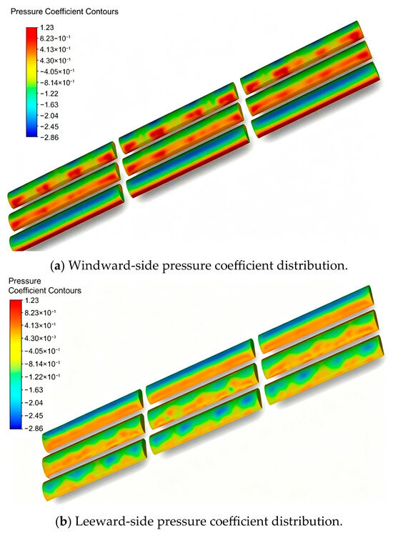
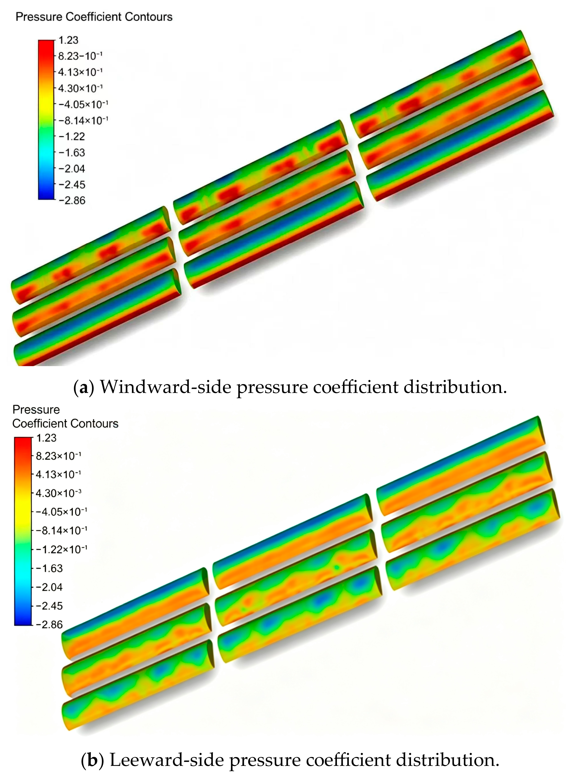
Figure 12 illustrates the pressure coefficient contours on Group 2 located in the valley topography.

Figure 12. Wind pressure coefficient contours of Group 2 under the 0° wind direction.

Figure 12 reveals a clear trend: compared with the 2 × 3 arrangement, the 3 × 3 layout exhibits more pronounced aerodynamic interference effects due to the increased cluster density.

As a result, the middle-row greenhouses experience highly non-uniform pressure distributions. This suggests that intermediate greenhouse positions may be subjected to complex localized loading conditions despite lower mean wind pressure values.

5.5.2. Comparison of C_p on Group 2 in Valley Areas and Plain Terrains

Table 8 shows the ratios of wind pressure coefficients of Group 2 in the valley terrain to those from the single-greenhouse flat-terrain case shown in Figure 9.

Table 8. Ratios of the C_p between valley topography and the plain region.

Shed Number	LF	MF	RF	LB	MB	RB	LW1	LW2	LW3	RW1	RW2	RW3	LT1	MT1	RT1	LT2	MT2	RT2	LT3	MT3	RT3
1	1.015	1.013	1.011	1.474	−0.064	0.660	0.966	0.747	0.621	1.031	1.031	1.103	0.985	0.992	1.008	0.995	0.993	1.013	1.133	0.968	1.015
2	1.011	1.013	1.013	−0.514	0.989	0.997	1.013	1.040	1.016	0.988	1.086	0.960	1.007	0.984	0.990	1.008	0.988	0.995	1.005	0.976	0.985
3	1.011	1.014	1.016	−0.727	3.173	0.102	1.089	1.011	1.126	0.963	0.802	0.694	0.992	0.989	0.976	0.995	0.995	0.984	0.875	0.965	1.018
4	4.285	0.436	3.568	4.348	1.138	0.757	1.615	1.844	2.421	1.286	1.331	1.044	2.162	1.269	0.810	1.021	0.982	0.996	0.845	1.167	0.761
5	0.926	0.380	0.322	0.368	2.062	1.269	1.147	1.155	1.269	1.112	1.218	1.465	0.755	0.613	0.585	1.056	0.878	0.970	1.004	0.884	1.079
6	0.584	2.005	3.955	0.238	0.066	2.161	0.853	0.941	0.977	1.121	1.157	1.296	0.940	0.714	−1.146	0.999	0.961	1.065	0.913	0.833	0.954
7	0.939	1.703	1.830	0.885	0.699	0.905	0.896	0.816	0.821	0.815	0.957	0.865	3.072	1.318	1.513	0.952	0.945	0.904	0.839	0.751	0.940
8	0.893	0.813	4.483	0.970	1.288	1.066	1.134	1.012	0.885	1.303	1.123	1.019	0.503	1.421	0.983	0.915	0.840	0.933	0.893	0.856	0.964
9	1.031	0.544	2.037	1.299	1.007	1.024	0.605	0.954	0.965	1.118	1.025	0.982	0.865	1.139	0.040	0.877	0.995	0.942	0.912	0.929	0.871

Note: The $C_p$ ratio is defined as $C_{p,\mathrm{v}\mathrm{a}\mathrm{l}\mathrm{l}\mathrm{e}\mathrm{y}}/C_{p,\mathrm{p}\mathrm{l}\mathrm{a}\mathrm{i}\mathrm{n}}$. When $C_{p,\mathrm{p}\mathrm{l}\mathrm{a}\mathrm{i}\mathrm{n}}$ is close to zero, the ratio becomes numerically sensitive and should be interpreted together with the corresponding original $C_p$ values. Large or negative ratios do not necessarily indicate proportional amplification or reduction in the physical wind pressure; further discussion is provided in Section 5.7.

Comparison between valley terrain and plain terrain results indicates that the influence of terrain becomes more evident in densely arranged greenhouse clusters.

In the 3 × 3 configuration, some interior greenhouses exhibit significant variation in C_p values compared with flat-terrain results. For certain roof regions, the absolute values of C_p in valley terrain exceed those observed in plain terrain, indicating that large ratios should be interpreted as local pressure redistribution, not as direct evidence of a specific vortex mechanism.

Although the overall wind exposure of interior greenhouses is reduced by shielding from the upstream rows, some local regions still exhibit large $C_p$ ratios, as observed for Shed 4 in Group 2. These ratios should be interpreted together with the corresponding original $C_p$ values and do not necessarily indicate proportional amplification of the total wind load. The numerical sensitivity associated with small denominators is discussed in Section 5.7.

5.5.3. Calculation of the Shape Factor of the Wind Load

The shape factors of the wind load on each surface of Group 2 are obtained, as shown in Table 9. While the corresponding correction coefficients relative to the Chinese Load Code are provided in Table A2 of Appendix B.

Table 9. Shape factor of the wind load of Group 2 in valley topography.

Shed Number	F	B	T1	T2	T3
1	0.970	−0.010	−0.860	−1.780	−0.290
2	0.994	−0.011	−0.887	−1.818	−0.282
3	0.971	0.011	−0.863	−1.793	−0.282
4	0.021	−0.010	0.000	−1.130	−0.266
5	0.016	−0.140	−0.044	−1.146	−0.342
6	0.030	0.007	0.009	−1.145	−0.264
7	0.078	−0.244	−0.082	−1.287	−0.630
8	0.067	−0.404	−0.158	−1.306	−0.743
9	0.099	−0.253	−0.079	−1.312	−0.648
Chinese Code GB/T 51183-2016 [28]	0.800	−0.500	0.143	−0.800	−0.500
USA NGMA 2004 [37]	0.800	−0.500	0.106	−0.971	−0.500
EU EN 13031-1:2019 [38]	0.600	−0.300	0.300	−1.000	−0.400
Korea MAFRA 1999 [39]	0.800	−0.400	−0.600	−0.7–−0.5	−0.200

Compared with the 2 × 3 arrangement, in the simulated 3 × 3 case, several interior greenhouses showed lower area-averaged shape factors than the boundary greenhouses. This suggests a shielding effect in selected interior regions, while exposed boundary and roof zones remain important for design interpretation.

The correction coefficients indicate that terrain effects may either amplify or reduce local wind loads depending on greenhouse position within the cluster. In particular, interior greenhouses experience strong aerodynamic interference effects, leading to significant deviation from flat-terrain design assumptions.

5.6. Analysis of the Simulation Results of Group 3 (3 × 5 Arrangement)

5.6.1. Pressure Coefficient Contours on Group 3 in the Valley Area

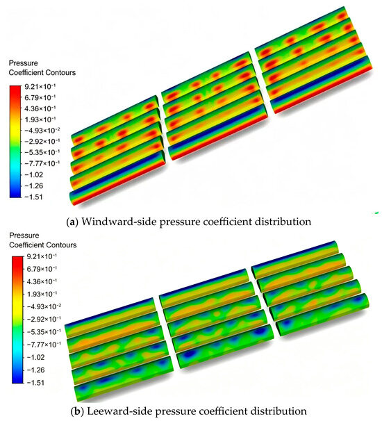
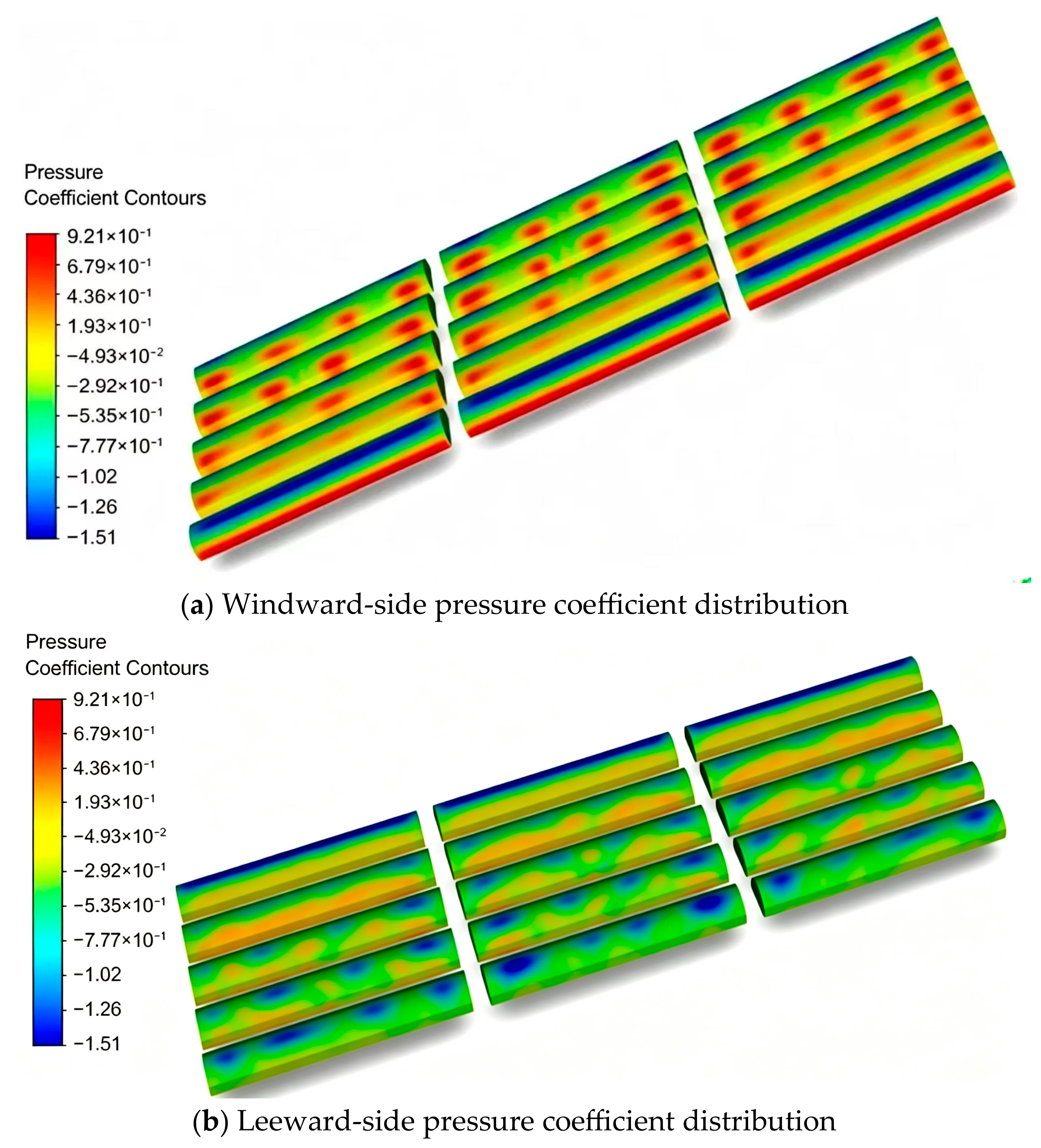
The pressure coefficient contours of Group 3 in valley terrain are shown in Figure 13.

Figure 13. Wind pressure coefficient contours of Group 3 under the 0° wind direction.

Figure 13 indicates that array shielding can reduce the area-averaged wind load in some interior greenhouse regions. However, this does not imply a general design benefit for larger arrays, because the governing wind loads are usually controlled by the most adverse local or zone-averaged pressure coefficients on exposed windward, eave, and roof suction regions.

5.6.2. Comparison of C_p on Group 3 in Valley Areas and Plain Terrains

Table 10 shows the ratios of wind pressure coefficients of Group 3 in valley terrain compared to those from the single-greenhouse flat-terrain case shown in Figure 9.

Table 10. Ratios of the C_p between valley topography and the plain region.

Shed Number	LF	MF	RF	LB	MB	RB	LW1	LW2	LW3	RW1	RW2	RW3	LT1	MT1	RT1	LT2	MT2	RT2	LT3	MT3	RT3
1	1.001	1.001	1.001	1.019	0.993	1.036	0.998	0.994	1.009	1.001	1.003	0.995	1.009	1.009	1.009	1.005	1.004	1.005	1.010	1.004	1.011
2	1.001	1.001	1.001	0.943	0.974	0.976	1.000	1.004	1.008	1.008	1.012	1.022	1.007	1.006	1.009	1.002	1.002	1.005	0.996	0.999	1.008
3	1.001	1.000	1.001	1.082	1.033	1.039	1.003	1.013	1.016	1.001	1.001	1.009	1.012	1.011	1.011	1.007	1.006	1.006	1.017	1.012	1.014
4	1.003	0.991	1.106	0.961	1.006	0.942	1.029	1.039	1.075	0.996	1.011	1.051	1.002	1.142	0.994	1.008	1.010	1.009	1.012	1.027	1.027
5	0.935	0.982	0.845	0.611	0.879	0.696	0.963	1.019	1.128	1.019	1.060	1.047	0.980	0.990	0.959	1.004	1.000	1.008	1.031	1.028	1.021
6	1.015	1.023	1.028	0.850	0.954	0.921	1.000	1.022	1.067	1.016	1.025	1.054	0.971	1.191	0.978	1.009	1.015	1.013	1.025	1.054	1.043
7	1.009	1.038	1.012	0.606	0.849	1.004	1.018	1.021	1.022	1.014	0.991	1.033	0.930	1.840	0.947	1.020	1.005	1.019	0.979	0.978	1.028
8	1.033	1.022	0.980	0.922	0.991	0.865	1.029	1.003	0.997	1.003	1.050	1.023	1.038	0.984	0.720	1.005	1.009	1.008	1.020	1.042	0.991
9	0.993	0.987	1.013	0.975	0.880	0.846	1.018	1.043	1.000	1.004	1.009	1.012	0.888	1.257	0.939	1.013	1.022	1.033	1.013	1.015	0.967
10	0.966	1.059	1.122	0.814	0.964	0.901	0.996	1.004	1.025	0.998	0.984	1.018	1.023	1.412	0.738	1.006	1.001	1.015	0.939	0.953	0.976
11	0.963	1.111	1.227	0.928	0.989	1.099	1.004	0.993	0.990	1.032	1.000	0.978	1.026	1.131	0.960	1.000	1.007	0.990	0.966	1.038	0.972
12	1.015	0.323	0.995	0.950	0.793	0.481	0.983	0.978	1.012	0.989	1.004	1.020	1.083	1.088	0.979	1.012	1.033	1.011	0.972	0.912	0.914
13	0.812	0.789	1.283	1.071	1.144	1.017	0.988	0.998	1.007	1.014	1.038	1.029	1.556	0.967	0.920	0.995	0.957	1.034	0.989	1.003	1.037
14	0.855	1.343	0.645	1.067	1.059	1.076	1.028	1.047	1.034	1.029	1.036	1.006	1.019	0.890	1.211	0.974	1.004	0.961	0.982	1.020	0.973
15	0.992	0.894	0.806	1.025	1.007	1.005	1.016	1.030	1.009	1.012	1.004	0.993	1.002	0.908	1.241	1.018	0.984	0.992	1.026	0.931	0.959

Note: The $C_p$ ratio is defined as $C_{p,\mathrm{v}\mathrm{a}\mathrm{l}\mathrm{l}\mathrm{e}\mathrm{y}}/C_{p,\mathrm{p}\mathrm{l}\mathrm{a}\mathrm{i}\mathrm{n}}$. When $C_{p,\mathrm{p}\mathrm{l}\mathrm{a}\mathrm{i}\mathrm{n}}$ is close to zero, the ratio becomes numerically sensitive and should be interpreted together with the corresponding original $C_p$ values. Large or negative ratios do not necessarily indicate proportional amplification or reduction in the physical wind pressure; further discussion is provided in Section 5.7.

In the 3 × 5 configuration, shielding by upstream greenhouses reduces the direct wind exposure of some interior greenhouses, which may lower the area-averaged wind–load response in selected regions. However, this shielding effect does not eliminate terrain-induced local pressure redistribution. Local C_p ratios may still show large values in specific surface regions because of small baseline C_p values, sign changes, wake interaction, and terrain-modified inflow. Therefore, the C_p ratios should be interpreted together with the original C_p values and area-averaged shape factors.

5.6.3. Calculation of Shape Factor of Wind Load

The shape factors of the wind load on each surface of Group 3 are shown in Table 11, with the corresponding correction coefficients relative to the Chinese Load Code given in Table A3 of Appendix B.

Table 11. Shape factor of the wind load of Group 3 in valley topography.

Shed Number	F	B	T1	T2	T3
1	0.952	−0.041	−0.646	−1.489	−0.234
2	0.969	−0.032	−0.646	−1.483	−0.218
3	0.951	−0.041	−0.647	−1.493	−0.237
4	−0.036	0.054	0.038	−0.793	−0.140
5	−0.035	0.015	0.022	−0.789	−0.166
6	−0.028	0.041	0.037	−0.788	−0.148
7	0.116	−0.041	0.054	−0.753	−0.246
8	0.094	−0.113	0.023	−0.780	−0.375
9	0.119	−0.067	0.044	−0.745	−0.275
10	0.086	−0.070	−0.003	−0.833	−0.356
11	0.094	−0.160	−0.044	−0.887	−0.499
12	0.094	−0.079	−0.021	−0.816	−0.346
13	0.058	−0.230	−0.056	−1.039	−0.583
14	0.084	−0.320	−0.088	−1.040	−0.670
15	0.043	−0.230	−0.071	−1.017	−0.566
Chinese Code GB/T 51183-2016 [28]	0.800	−0.500	0.143	−0.800	−0.500
USA NGMA 2004 [37]	0.800	−0.500	0.106	−0.971	−0.500
EU EN 13031-1:2019 [38]	0.600	−0.300	0.300	−1.000	−0.400
Korea MAFRA 1999 [39]	0.800	−0.400	−0.600	−0.7–−0.5	−0.200

Compared with the 2 × 3 and 3 × 3 arrangements, in the simulated 3 × 5 case, several interior greenhouses showed lower area-averaged shape factors than boundary greenhouses. This suggests a shielding effect in selected interior regions, while exposed boundary and roof zones remained important for design interpretation. However, boundary greenhouses still experience relatively large wind loads, particularly on windward and roof surfaces. Roof regions exhibit the largest absolute shape factor values among all greenhouse surfaces, indicating that uplift effects remain critical for greenhouse safety.

Overall, the 3 × 5 configuration demonstrates that increasing cluster density enhances aerodynamic shielding.

5.7. Interpretation of C_p Ratios and Numerical Uncertainty

The ratios $C_{p,\mathrm{v}\mathrm{a}\mathrm{l}\mathrm{l}\mathrm{e}\mathrm{y}}/C_{p,\mathrm{p}\mathrm{l}\mathrm{a}\mathrm{i}\mathrm{n}}$ reported in Table 6, Table 8 and Table 11 are used only as case-specific descriptive indicators of the differences between the valley terrain and plain-terrain simulations. These ratios are sensitive to the magnitude and sign of $C_{p,\mathrm{p}\mathrm{l}\mathrm{a}\mathrm{i}\mathrm{n}}$. When the absolute value of $C_{p,\mathrm{p}\mathrm{l}\mathrm{a}\mathrm{i}\mathrm{n}}$ is close to zero, even a small absolute difference between the two coefficients may produce a large positive or negative ratio. A change in sign between the two cases may also produce a negative ratio. Therefore, large or negative ratio values should not be interpreted directly as proportional amplification or reduction in the physical wind pressure or structural wind load.

To avoid overinterpretation, the ratio values are considered together with the corresponding original $C_p$ values. Particular attention is given to whether the denominator is close to zero, whether both coefficients have small absolute magnitudes, and whether a sign change occurs between the two terrain cases. Ratios associated with small denominators are therefore treated as numerically sensitive indicators of local pressure redistribution rather than as direct terrain-induced wind load amplification factors. A normalized difference based on the difference between the two $C_p$ values divided by their mean may provide a more robust comparison and will be considered in future studies.

From the perspective of numerical uncertainty, local wind pressure coefficients are more sensitive to mesh resolution, near-wall treatment, convergence criteria, and local flow separation than area-averaged quantities. During the CFD simulations, convergence was assessed based on residual reduction and stabilization of monitored pressure quantities. Although the same mesh strategy, turbulence model, boundary conditions, and convergence criteria were adopted for the plain-terrain and valley terrain cases to ensure comparability, the ratios associated with small denominators were interpreted with caution. Future work should further quantify numerical uncertainty through a systematic greenhouse-scale mesh sensitivity analysis and uncertainty assessment.

The local maximum and minimum C_p values shown in Figure 9, Figure 11, Figure 12 and Figure 13 represent pointwise extrema extracted from different greenhouse configurations and do not necessarily occur at the same surface region, greenhouse position, or aerodynamic condition. Therefore, these extrema are not used as a direct like-for-like comparison of structural design loads. They are reported only to indicate the overall range of the contour results and to explain the apparent differences among the color scales. The design interpretation should be based primarily on the zone-averaged pressure coefficients and wind load shape factors.

The comparison indicates that the greenhouse-array cases may produce larger local positive C_p values on exposed windward or front stagnation regions, whereas the single-greenhouse plain-terrain case can still show stronger local roof suction. This does not indicate an inconsistency in reference wind speed or reference pressure, because all C_p values were normalized using the same definition. Instead, it reflects the redistribution of pressure caused by array interference, shielding, gap flow, terrain-modified incoming flow, and local acceleration or separation over the arched roof.

It should also be noted that the absence of an independent greenhouse-scale mesh sensitivity analysis may introduce uncertainty in local pointwise pressure extrema, especially in roof-edge, windward-wall, and wake-affected regions. Therefore, local extreme C_p values and ratio-based indicators should be interpreted together with area-averaged shape factors and the overall comparative trends among cases.

5.8. Comparative Discussion of Different Cluster Arrangements

A comparative analysis of Groups 1, 2, and 3 suggests that the simulated C_p and shape-factor distributions are influenced by both terrain-modified inflow and greenhouse-array arrangement. Roof regions showed relatively large suction coefficients in the simulated cases, but the specific flow mechanisms require further verification using velocity-field analysis, transient simulations, or experimental data.

As cluster density increases from 2 × 3 to 3 × 3 and then to 3 × 5, aerodynamic shielding becomes progressively stronger. This reduces the windward pressure acting on interior greenhouses and lowers the direct wind exposure of downstream structures.

The CFD-predicted pressure coefficient distributions show larger deviations from the single-greenhouse level-terrain reference on the first-row and peripheral greenhouses. For interior greenhouses, the pressure patterns are influenced by surrounding greenhouse rows, indicating that the differences reflect the combined effects of terrain-modified inflow and array interference. Therefore, the present results should not be interpreted as isolating the effect of valley topography alone.

The comparison suggests that the simulated C_p and shape-factor distributions reflect the combined influence of terrain-modified inflow and greenhouse-array arrangement. Because no independent experimental data are available for the array cases, these results should be interpreted as CFD-based trends rather than direct evidence of a fully resolved terrain–structure interaction mechanism.

The symbols used in this paper and their definitions are presented in Table A4 of Appendix C.

6. Conclusions and Future Work

6.1. Conclusions

This study investigated the wind load characteristics of plastic greenhouse clusters located in valley terrain using CFD simulation, with emphasis on the combined effects of terrain-induced wind field variation and aerodynamic interference between adjacent structures. The main conclusions are summarized as follows:

• In the selected CFD cases, the valley terrain inflow condition led to noticeable differences in the simulated wind pressure coefficient distribution on greenhouse surfaces, resulting in noticeable deviations from those under flat-terrain conditions. Compared with flat-terrain assumptions, noticeable deviations in wind load shape factors are observed, particularly in windward walls, roof regions, and leeward surfaces.
• Greenhouses located in the first row and outermost positions consistently experience the largest wind loads because they are directly exposed to approaching airflow and less affected by aerodynamic shielding.
• The CFD-based relative ratios and shape-factor differences obtained in this study quantify the deviation between the selected valley terrain cases and the corresponding reference cases. These values are site-specific and should not be used as generally applicable design coefficients without further verification.

6.2. Limitations of the Study

While this study provides a systematic evaluation of wind load characteristics for greenhouse clusters in valley terrain, several limitations should be acknowledged. A primary focus of the comparative analysis was directed toward the Chinese wind loading codes. This specific focus is dictated by the geographic location of the case study (Tibet, China) and the practical necessity for local engineers to adhere to regional safety standards and construction mandates.

In addition, only the 0° wind direction was considered as a representative unfavorable normal-wind case for evaluating the overall wind resistance of single-span greenhouses. However, under complex valley terrain conditions, oblique winds may produce stronger local suction, asymmetric pressure distributions, and torsional effects on edge greenhouses and roof corner regions. The associated mechanisms should be examined in future studies using additional wind directions and flow-field analysis. Therefore, the present results primarily represent the aerodynamic characteristics under the selected 0° normal wind direction and should not be regarded as covering all possible critical wind directions.

It should also be noted that the present numerical validation and analysis were based on mean wind pressure coefficients. Fluctuating and peak wind pressures were not evaluated in this study. Since the steady Reynolds-averaged Navier–Stokes (RANS) approach mainly predicts time-averaged flow quantities, it cannot fully resolve unsteady vortex shedding and transient pressure fluctuations around greenhouse structures, particularly in leeward roof and wake regions. Therefore, the obtained wind pressure coefficients and shape factors should be interpreted as mean wind load characteristics. Future studies should employ transient methods, such as URANS or LES, or wind tunnel measurements to further investigate fluctuating and peak wind pressure characteristics of arched greenhouse clusters in complex valley terrain.

In addition, although the greenhouse cluster meshes were generated using a consistent refinement strategy and local mesh refinement was applied near the greenhouse surfaces, an independent mesh sensitivity study for the greenhouse-scale simulations was not conducted in the present work. Therefore, mesh-induced uncertainty in the local pressure coefficients and wind load shape factors could not be quantified explicitly. The comparative results among different terrain and layout cases should be interpreted within the same numerical framework. Future work should conduct systematic greenhouse-scale mesh sensitivity analyses to further evaluate the influence of mesh resolution on local pressure extrema and area-averaged wind load shape factors.

The present CFD simulations are based on several idealized assumptions, including prescribed inflow conditions, dry and neutral atmospheric conditions, and the neglect of surface energy balance effects and Coriolis forces. These simplifications should be considered when interpreting the results.

However, we recognize that this regional focus may limit the direct numerical applicability of the correction factors to other international standards. The primary contribution of this work is the demonstration of a CFD-based workflow for examining how terrain-modified inflow and greenhouse-array arrangement affect mean pressure coefficients in a selected valley case. The resulting numerical values and aerodynamic trends are specific to the selected terrain geometry, greenhouse layout, wind direction, and numerical modeling assumptions.

6.3. Future Work

• Oblique wind directions or a staggered arrangement of greenhouses may cause asymmetric wind pressure coefficient distribution on the greenhouse envelope, leading to torsional effects or local stress concentrations, which are critical for the structural safety of plastic greenhouses. In future studies, we will extend research on staggered arrangements and oblique wind directions, which can enrich the understanding of wind-induced interference effects in plastic greenhouse clusters and provide more comprehensive and reliable technical support for the wind-resistant design and safety assessment of such structures.
• Steady-state simulations ignore the aeroelastic effect of flexible covers. Future work should verify results via 1:50 scaled wind tunnel tests (for the three layouts) to evaluate the CFD-predicted aerodynamic trends observed in the present study.
• In addition, the effects of local surrounding obstacles, such as nearby buildings and vegetation, were not considered in the current study and should be incorporated in future simulations to improve site-specific wind load assessment.

References

- Bowen, A.J.; Lindley, D. A wind-tunnel investigation of the wind speed and turbulence characteristics close to the ground over various escarpment shapes. Bound.-Layer Meteorol. 1977, 12, 259–271. [Google Scholar] [CrossRef] [Scilit]
- Kwon, K.S.; Lee, I.B.; Kim, R.W.; Seo, I.H. Evaluation of wind pressure coefficients of single-span greenhouses built on reclaimed coastal land using a large-sized wind tunnel. Biosyst. Eng. 2016, 141, 58–81. [Google Scholar] [CrossRef] [Scilit]
- Maraveas, C. Wind Pressure Coefficients on Greenhouse Structures. Agriculture 2020, 10, 149. [Google Scholar] [CrossRef] [Scilit]
- Xu, J.; He, G.; Ren, X.; Hu, Z. Research on wind pressure coefficient distribution of plastic greenhouses in valley topography. Eng. Agríc. 2022, 42, e20220075. [Google Scholar] [CrossRef] [Scilit]
- Gao, Z.; Xu, J.; Wang, R.; Jiang, Y.; Liang, Z. Study of Wind Field and Surface Wind Pressure of Solar Greenhouse Group under Valley Topography Conditions. Agronomy 2024, 14, 973. [Google Scholar] [CrossRef] [Scilit]
- Charisi, S.; Thiis, T.K.; Aurlien, T. Full-Scale Measurements of Wind-Pressure Coefficients in Twin Medium-Rise Buildings. Buildings 2019, 9, 63. [Google Scholar] [CrossRef] [Scilit]
- Lee, E.-J.; Hwang, S.-K.; Kim, D.-W.; Ha, Y.-C. Characteristic of Vertical Distributions of Mean Wind Pressure for Windward and Leeward Walls of Tall Buildings. J. Archit. Inst. Korea Struct. Constr. 2008, 24, 35–42. Available online: http://journal.auric.kr/jaik_sc/ArticleDetail/RD_R/215895 (accessed on 2 July 2024).
- Park, J.H.; Chung, Y.B.; Ha, Y.C. A proposal of the wind pressure coefficient and simplified wind load estimating formula for the design of structural frames of the low-rise buildings. J. Korean Soc. Steel Constr. 2009, 21, 289–299. [Google Scholar]
- Kim, Y.C.; Tamura, Y. Simulation of Wind Pressures on a Target Low-Rise Building in Large Group by RANS Turbulence Model. J. Aerosp. Eng. 2015, 28, 04014082. [Google Scholar] [CrossRef] [Scilit]
- Bartko, M.; Molleti, S.; Baskaran, A. In situ measurements of wind pressures on low slope membrane roofs. J. Wind Eng. Ind. Aerodyn. 2016, 153, 78–91. [Google Scholar] [CrossRef] [Scilit]
- You, J.-Y.; Kim, G.-H.; Chae, M.-J. Analysis of peak wind pressure coefficients of penetration type and end type pilots. J. Korean Assoc. Spat. Struct. 2018, 18, 59–67. [Google Scholar] [CrossRef] [Scilit]
- Li, S.H.; Kilpatrick, J.; Browne, M.T.L.; Yakymyk, W.; Refan, M. Uncertainties in Prediction of Local Peak Wind Pressures on Mid- and High-Rise Buildings by Considering Gumbel Distributed Pressure Coefficients. J. Wind Eng. Ind. Aerodyn. 2020, 206, 104364. [Google Scholar] [CrossRef] [Scilit]
- Kandel, A.; Sun, X.; Wu, Y. Wind Tunnel Experiment on Rectangular-Shaped Arch-Supported Membrane Structures. Structures 2022, 41, 1515–1531. [Google Scholar] [CrossRef] [Scilit]
- Bronkhorst, A.J.; Geurts, C.P.W.; van Bentum, C.A.; van der Knaap, L.P.M.; Pertermann, I. Wind Loads for Stability Design of Large Multi-Span Duo-Pitch Greenhouses. Front. Built Environ. 2017, 3, 18. [Google Scholar] [CrossRef] [Scilit]
- Kim, R.U.; Kim, D.W.; Ryu, K.C.; Kwon, K.S.; Lee, I.B. Estimation of wind pressure coefficients on even-span greenhouse built in reclaimed land according to roof slope using wind tunnel. Prot. Hortic. Plant Fact. 2014, 23, 269–280. [Google Scholar] [CrossRef] [Scilit]
- Rosa, R.J.; Hincz, K. Investigation of Wind Loading on a Multi-span Anticlastic Tensile Membrane Surface: A CFD Approach. Period. Polytech. Civ. Eng. 2025, 69, 1092–1107. [Google Scholar] [CrossRef] [Scilit]
- Kuroyanagi, T. Investigating air leakage and wind pressure coefficients of single-span plastic greenhouses using computational fluid dynamics. Biosyst. Eng. 2017, 163, 15–27. [Google Scholar] [CrossRef] [Scilit]
- Liang, Z.; Gao, Z.; Li, Y.; Zhao, S. Study on the effect of size on the surface wind pressure and shape factor of wind load of solar greenhouses. Appl. Sci. 2024, 14, 7114. [Google Scholar] [CrossRef] [Scilit]
- Castro, I.P.; Robins, A.G. The flow around a surface-mounted cube in uniform and turbulent streams. J. Fluid Mech. 1977, 79, 307–335. [Google Scholar] [CrossRef] [Scilit]
- Holmes, J.D. Wind Loading of Structures, 3rd ed.; CRC Press: Boca Raton, FL, USA, 2015. [Google Scholar]
- Fernández-García, M.S.; Vidal-López, P.; Rodríguez-Robles, D.; Villar-García, J.R.; Agujetas, R. Numerical Simulation of Multi-Span Greenhouse Structures. Agriculture 2020, 10, 499. [Google Scholar] [CrossRef] [Scilit]
- Kim, R.-W.; Lee, I.-B.; Yeo, U.-H.; Lee, S.-Y. Estimating the wind pressure coefficient for single-span greenhouses using an large eddy simulation turbulence model. Biosyst. Eng. 2019, 188, 114–135. [Google Scholar] [CrossRef] [Scilit]
- Blocken, B. 50 years of computational wind engineering: Past, present and future. J. Wind Eng. Ind. Aerodyn. 2014, 129, 69–102. [Google Scholar] [CrossRef] [Scilit]
- Kim, R.; Lee, I.; Kwon, K. Evaluation of wind pressure acting on multi-span greenhouses using CFD technique, Part 1: Development of the CFD model. Biosyst. Eng. 2017, 164, 235–256. [Google Scholar] [CrossRef] [Scilit]
- Kim, R.; Hong, S.; Lee, I.; Kwon, K. Evaluation of wind pressure acting on multi-span greenhouses using CFD technique, Part 2: Application of the CFD model. Biosyst. Eng. 2017, 164, 257–280. [Google Scholar] [CrossRef] [Scilit]
- Liang, Z.; He, G.; Li, Y.; Gao, Z. Analysis of wind pressure coefficients for single-span arched plastic greenhouses located in a valley region using CFD. Agronomy 2023, 13, 553. [Google Scholar] [CrossRef] [Scilit]
- Xu, J.; Ren, X.; He, G.; Di, S. The influence of mountain height and distance on shape factor of wind load of plastic tunnel. Appl. Sci. 2023, 13, 13081. [Google Scholar] [CrossRef] [Scilit]
- GB/T 51183-2016; Code for the Design Load of Horticultural Greenhouse Structures. China Planning Press: Beijing, China, 2016.
- JGJ/T 481-2019; Standard for Wind Loads on Roof Structures. China Architecture & Building Press: Beijing, China, 2020.
- Fu, W.; Li, M.; Yin, S.; Lv, Z.; Wang, L. Study on the atmospheric boundary layer structure of the Qinghai-Xizang Plateau under the south branch of the westerly wind and the plateau monsoon circulation field. Plateau Meteorol. 2022, 41, 190–203. [Google Scholar] [CrossRef]
- GB 50009-2012; Load Code for the Design of Building Structures. China Architecture & Building Press: Beijing, China, 2012.
- Guo, X. Study on Thermal Performance of the Heating Radiator in Cold Regions with High Altitude. Master’s Thesis, Chongqing University, Chongqing, China, 2014. [Google Scholar]
- Huang, B.; Wang, C. Principles and Applications of Structural Wind Resistance Analysis; Tongji University Press: Shanghai, China, 2008. [Google Scholar]
- Murakami, S.; Mochida, A. 3-D numerical simulation of airflow around a cubic model by means of the k-model. J. Wind Eng. Ind. Aerodyn. 1988, 31, 283–303. [Google Scholar] [CrossRef] [Scilit]
- Richards, P.; Hoxey, R. Pressures on a cubic building-part 1: Full-scale results. J. Wind Eng. Ind. Aerodyn. 2012, 102, 72–86. [Google Scholar] [CrossRef] [Scilit]
- Li, L.; Zhang, L.; Zhang, N.; Hu, F.; Jiang, Y.; Jiang, W. Application of FLUENT on the fine-scale simulation of the wind field over complex terrain. Plateau Meteorol. 2010, 29, 621–628. [Google Scholar]
- NGMA. Structural Design Manual; National Greenhouse Manufacturers Association: Harrisburg, PA, USA, 2004. [Google Scholar]
- EN 13031-1; Greenhouses: Design and Construction—Part 1: Commercial Production Greenhouses. European Committee for Standardization: Brussels, Belgium, 2019.
- MAFRA. Standard and Explanation for Greenhouse Structural Design; Ministry of Agriculture, Food and Rural Affairs: Gwacheon, Republic of Korea, 1999.
Disclaimer/Publisher’s Note: The statements, opinions and data contained in all publications are solely those of the individual author(s) and contributor(s) and not of MDPI and/or the editor(s). MDPI and/or the editor(s) disclaim responsibility for any injury to people or property resulting from any ideas, methods, instructions or products referred to in the content. |
© 2026 by the authors. Licensee MDPI, Basel, Switzerland. This article is an open access article distributed under the terms and conditions of the Creative Commons Attribution (CC BY) license.