


Abstract
Fractures exert a significant influence on rock mass deformation and seepage pathways, thereby posing a serious challenge to the safe and efficient extraction of deep mines. This problem is particularly evident in deep mines located near the sea, where fractures are extensively developed. For such mines, the overlying seawater represents a considerable potential risk to mining safety. Therefore, investigating the distribution characteristics of deep fractures and clarifying the coupling relationships among the fracture, stress, seepage, and temperature fields are important for ensuring safe and efficient production in deep mines near the sea. Taking the auxiliary shaft of the Sanshandao Gold Mine as the engineering case, this study uses extensive measured fracture data, determines fracture locations by their centroids, and adopts kernel density estimation to non-parametrically characterize the fracture spatial distribution. Fourier convolution is then employed to rapidly reconstruct fracture positions in the discrete fracture network (DFN) model. The results demonstrate that the proposed kernel density estimation method can effectively identify the spatial distribution characteristics of fractures. Subsequently, the fracture field of the underground rock mass is reconstructed by the Monte Carlo method, and a thermal–hydro–mechanical multi-field coupling model incorporating the fracture field is established. The numerical results indicate that fluid flow is primarily concentrated along fractures, and that heat transfer within fractures is markedly faster than that in the rock matrix. The presence of fractures significantly affects the stress field of the underground rock mass, and their influence on the stress distribution increases as fracture length becomes greater. Accordingly, the effects of fractures should not be neglected in numerical analyses. The findings provide reliable support for mine stability calculations and safety evaluations.
1. Introduction
Natural rock masses commonly contain numerous fractures formed during geological evolution and further influenced by long-term engineering disturbances. These discontinuities not only modify the mechanical behavior of the rock mass, but also provide important pathways for groundwater flow and transport [1,2]. When distributed throughout the rock mass, they constitute complex fracture networks that are highly relevant to shale gas extraction [3], geothermal resource development, nuclear waste disposal, and other geological engineering applications [4,5,6]. Consequently, reliable identification of the spatial arrangement of fractures is essential for assessing the safety, stability, and hydraulic response of underground engineering systems. Nevertheless, accurately describing fracture networks at the engineering scale remains a considerable challenge. Field measurement of individual structural planes is itself demanding, whereas complete identification of all fractures within a rock mass is generally impractical.
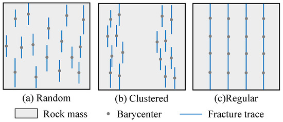
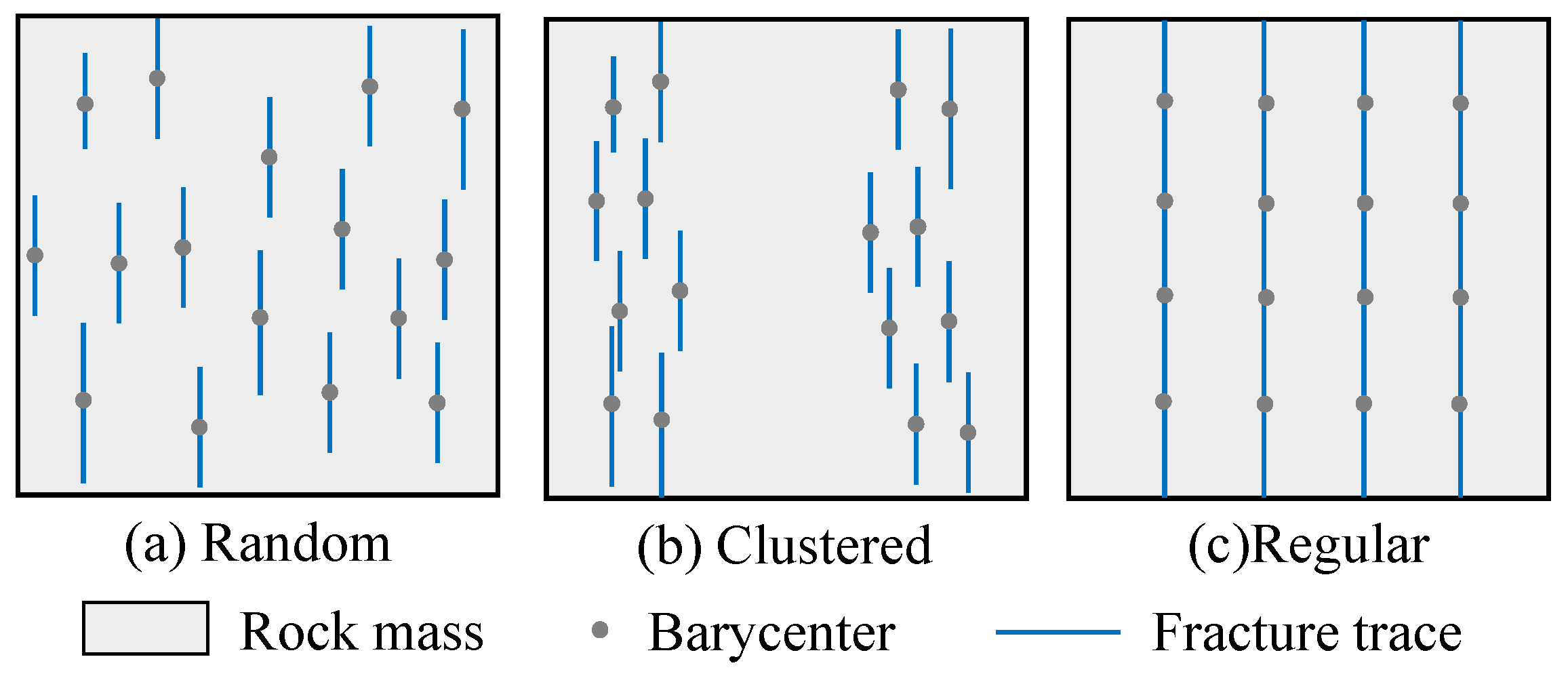
In engineering practice, fracture characteristics and their geological distribution are generally inferred from limited observations obtained through rock outcrops, borehole cores, borehole imaging, and geophysical exploration. A variety of statistical and stochastic methods have therefore been developed for fracture description and reconstruction. Zhang et al. [7] characterized the distribution of fracture lengths using a negative exponential function, while Xu et al. [8] introduced a statistical window sampling approach to improve the estimation of fracture trace lengths. Song et al. [9] subsequently developed a three-dimensional fracture-network simulation method by combining probability statistics, stochastic theory, and computer programming. Among the available approaches, the Discrete Fracture Network (DFN) model has become an important tool for representing three-dimensional fracture systems and has been widely applied in geotechnical and petroleum engineering research [10,11]. However, conventional DFN models commonly generate fractures according to a prescribed density under the assumption of spatial randomness, namely, the Poisson model [12]. Such an assumption does not adequately represent the spatial organization and correlation typically exhibited by fractures in natural rock masses. In reality, natural fractures may occur in clustered, regular, or random arrangements, as illustrated in Figure 1. In this figure, the blue lines denote fracture traces and the gray points indicate their centroids. Although the three cases have identical fracture numbers and comparable mean intensities, their different spatial arrangements lead to distinct structural characteristics. The spatial organization becomes even more complicated when several fracture sets occur simultaneously. Therefore, an accurate reconstruction of deeply fractured rock masses should describe not only the statistical characteristics of fracture geometry, but also the spatial distribution patterns and heterogeneity of the fracture network.
Figure 1.
Fracture distribution pattern.
For coastal mining operations, overlying seawater may constitute a major potential hazard to underground safety. As the mining depth approaches 2000 m, the effects of high in situ stress, elevated geothermal temperature, and high seepage pressure within deep rock masses become increasingly pronounced. Under these geological conditions, interactions among stress, fluid flow, temperature, and fracture evolution are important factors governing the stability and safety of deep underground engineering. Previous studies on underground energy-storage caverns have further demonstrated that excavation geometry, in situ stress conditions, and chamber configuration can significantly affect the stability and stress redistribution of surrounding rock masses [13,14]. Current numerical methods for analyzing coupled multi-field processes in deep geological engineering mainly include the finite difference method (FDM), boundary element method (BEM), finite element method (FEM), and finite volume method (FVM). Most available numerical platforms can simulate coupled seepage and heat-transfer processes [15,16,17,18], while several computational frameworks have further been developed for thermal–hydro–mechanical (THM) and thermal–hydro–mechanical–chemical (THMC) analyses. For instance, Rutqvist used TOUGH-FLAC to examine deformation and pore-pressure evolution in deep geological projects, including the In Salah CO2 storage project in Algeria and the Geysers geothermal field in the United States [19]. Kong et al. [20] proposed an optimization approach for geothermal well spacing based on OpenGeoSys, while programs such as ROLG can additionally account for liquid–gas phase transition and steam transport [21].
To better represent the complex behavior of fractured rock masses, discrete fracture models and mesoscopic simulation methods have also been incorporated into THM analyses. Pan et al. [22] applied cellular automata to rock-mechanics simulations and used weakened cellular elements to describe the mechanical response of complex fracture networks under THM coupling conditions. Sun et al. [23] developed a THM coupling model containing discrete fractures and compared heat-extraction performance under thermal-flow and THM coupling conditions, indicating the necessity of accounting for THM effects. Yao et al. [24] established a numerical model for heat extraction in Enhanced Geothermal Systems (EGS), examined the pressure, temperature, stress, and deformation distributions within geothermal reservoirs, and identified fractures as the principal flow pathways. Hofmann et al. [25] constructed a two-dimensional discrete fracture model for granite formations to evaluate the effects of fracture number, discretization, and well location on heat-extraction efficiency, and reported better performance for complex fracture networks than for simple horizontal fracture systems. Li et al. [26] proposed an open-loop dual-well heat-extraction model and showed that increasing well spacing could improve thermal recovery efficiency. From a broader modeling perspective, data-driven multiscale approaches have also been used to characterize crack initiation and evolution in heterogeneous solid materials under mechanical loading [27]. Although the material system considered in such studies differs from fractured rock masses, the corresponding multiscale description of crack evolution provides a useful methodological reference for analyzing damage localization in complex geological media.
Despite these advances in the analysis of THM processes in fractured rock masses, relatively limited attention has been given to coupled multi-field behavior induced by shaft excavation in deep coastal mining environments. In particular, the relationships among fracture distribution, stress redistribution, seepage migration, and temperature evolution under such conditions remain insufficiently understood. Therefore, accurately describing the spatial distribution of deep fracture networks and examining the coupling among fracture, stress, seepage, and temperature fields are important for the safe and efficient production of the deep coastal mines.
In this study, the deputy shaft in the Sanshandao mining area is taken as the engineering background. Based on a substantial amount of field-measured fracture data, fracture locations are represented by their centroids, and kernel density estimation (KDE) is adopted to describe the fracture spatial distribution in a non-parametric manner. Fourier convolution is subsequently applied to enable rapid reconstruction of fracture locations within the Discrete Fracture Network (DFN) framework. Using the obtained distribution characteristics, the underground fracture field is reconstructed by the Monte Carlo method. A thermal–hydro–mechanical multi-field coupling model incorporating the reconstructed fracture network is then developed in COMSOL6.2 to support stability analysis and safety evaluation for deep coastal mining engineering.
2. Reconstruction of Fracture Field
2.1. Overview of the Study Area
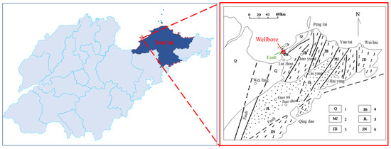
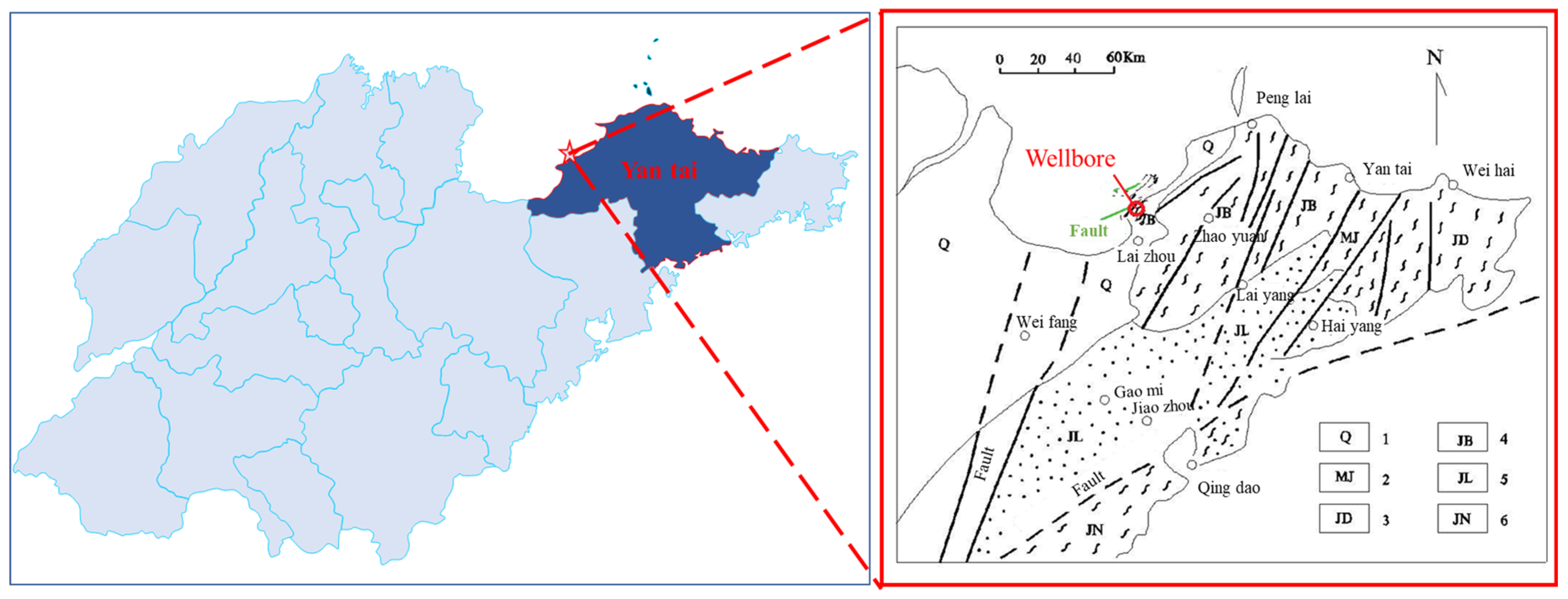
Sanshandao gold mining area is situated in Bohai Bay, and the shaft considered in this study is located at the foot of the mountain on the northwestern side of the Xishan mining area (Figure 2). The nearshore zone and seabed are generally low and flat, with elevations ranging from −5.8 m to +2.0 m. Three small hills occur close to the shoreline, among which the highest point reaches an elevation of +67.14 m; these hills are classified as denudational monadnocks. In contrast, the terrain along the eastern coastal area is relatively flat and gently inclined, with elevations between 2.0 m and 6.5 m. This area belongs to a coastal plain sedimentary landform, where eolian coarse sand is extensively distributed in the shallow surface layer. The ground surface is mainly covered by Quaternary deposits, beneath which lies the Neoarchean Jiaodong Group. The principal lithologies include granite, granodiorite, gneiss, monzonitic granite, and gneissic fine-grained biotite hornblende tonalite [28].
Figure 2.
Location of the study area.
The submarine topography along the eastern coast of Laizhou Bay is relatively simple. The 10 m isobath lies approximately 2–4 km offshore and generally follows the contour of the coastline. Beyond this isobath, the seabed becomes flat with only a gentle gradient, and the supply of terrigenous material is limited. The regional hydrodynamic conditions are mainly controlled by reciprocating currents in the NE–NW directions and waves from the north-by-west direction. Except for a small underwater delta developed at the mouth of the boundary river, nearshore underwater shoals are present and gradually transition seaward into a submarine accumulation plain.
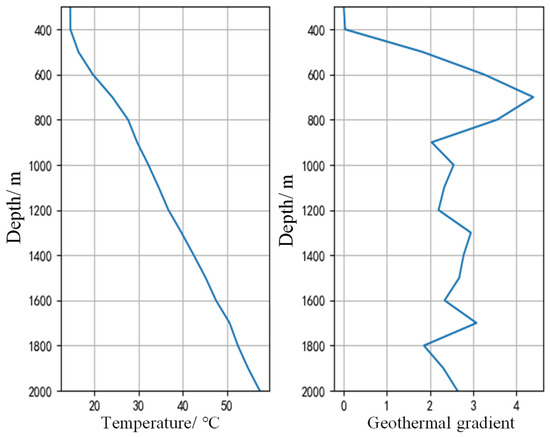
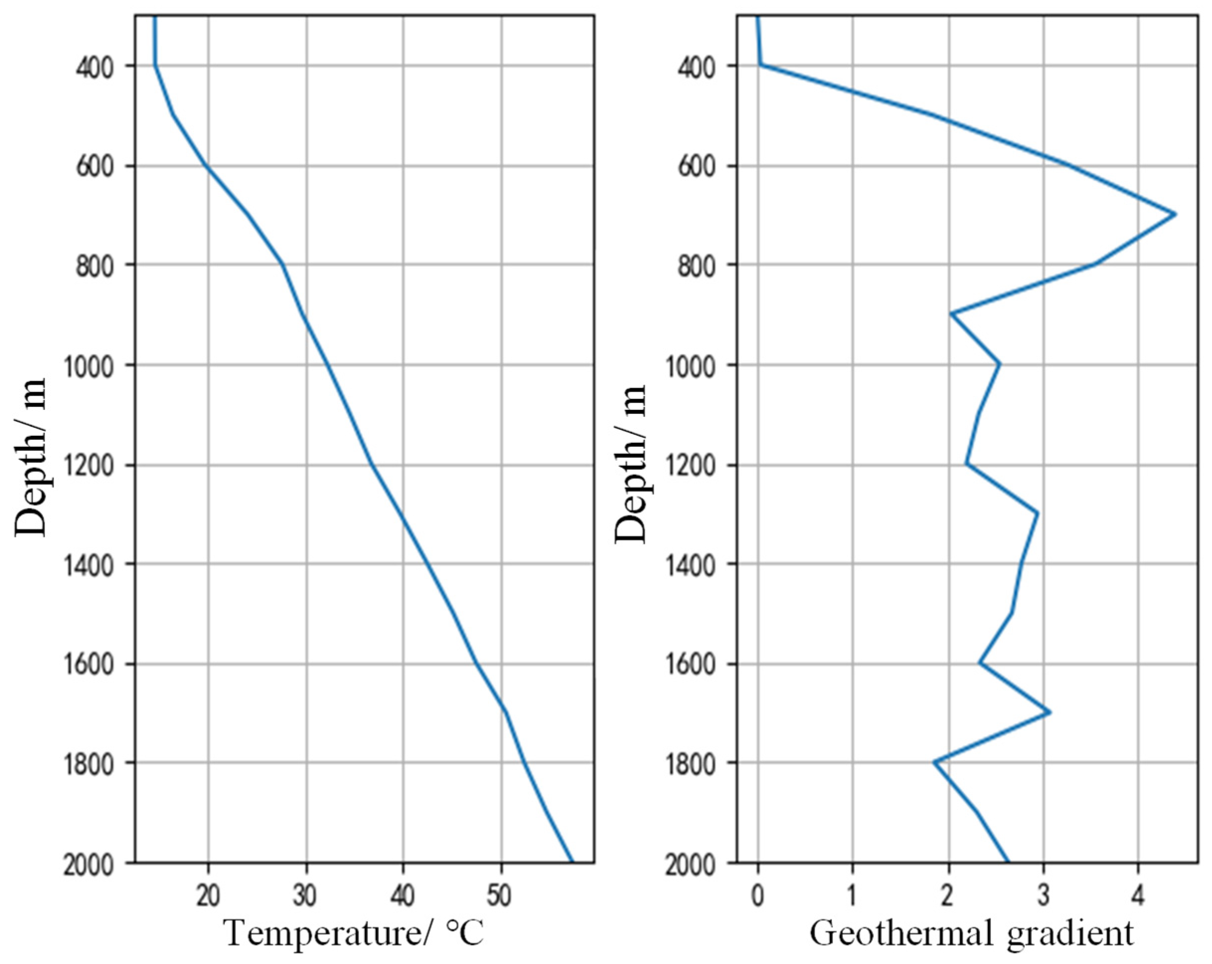
Fault structures constitute the principal tectonic features in the study area and can be classified as ore-controlling faults or post-ore faults according to their genetic relationships. Three faults, designated F1, F2, and F3, are developed within the area. The exposed rocks are dominated by magmatic and metamorphic rocks, most of which are connected through altered transitional contacts. No distinct structural planes are observed either between the different lithologies or within the rocks themselves. Accordingly, the main structural planes identified in the investigated area are fault-related structural planes. The average geothermal gradient is 2.4 °C per 100 m. The recorded temperature is 14.5 °C at a depth of 300 m and increases to 57 °C at a logging depth of 2000 m, indicating a high-temperature environment in the deep formation.
Kernel density estimation (KDE) is a non-parametric approach in which the probability density function is inferred directly from the observed samples rather than assumed to follow a predefined distribution. Therefore, a distribution model can be constructed from the intrinsic pattern of the available data without requiring prior information about the population form. Compared with parametric approaches, KDE reduces dependence on assumed sample distributions and is thus more suitable for describing data with random characteristics. For a one-dimensional real random variable X = {x1, x2, x3, …, xn}, the kernel density estimate is defined as follows [29]:
where h is the bandwidth, n denotes the sample numbers, xi represents the ith sample, and K is the kernel function.
The performance of KDE is primarily affected by the selected kernel function and bandwidth. Of these two factors, bandwidth generally has a more pronounced influence on the fitting result of the estimated distribution [30]. The bandwidth h controls the smoothing degree of the probability density curve: a larger value produces a smoother density estimate, whereas a smaller value preserves more local variation and leads to a sharper curve. In this study, the bandwidth is determined by minimizing the mean integrated squared error (MISE), as expressed below [31]:
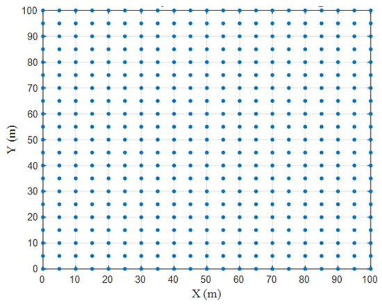
Because a fracture network generally contains a large number of fractures, performing statistical calculations for each individual fracture would impose a substantial computational burden. To improve computational efficiency, a fast kernel density estimation algorithm is adopted in this study, and new fracture points are subsequently generated from the estimated density distribution. In this procedure, the study domain is first divided linearly into equally spaced grids, as illustrated in Figure 3. Each measured data point is then traversed and assigned to its neighboring grid vertices with corresponding weights. In the one-dimensional case, a data point contributes weights to the two nearest grid vertices; for a d-dimensional case, weights are allocated to the adjacent 2d grid vertices. The computational complexity of this assignment process is therefore O(n2d). Fourier discrete convolution is subsequently employed to calculate the kernel density estimate, requiring a total of O(nlogn) operations, where n represents the number of grid points. When the statistical region is sufficiently large to reflect fracture distribution throughout the study domain, the estimated kernel density values can be used to characterize the spatial structure of fractures in the entire region.
Figure 3.
Equidistant grid points used for kernel density sampling.
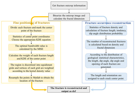
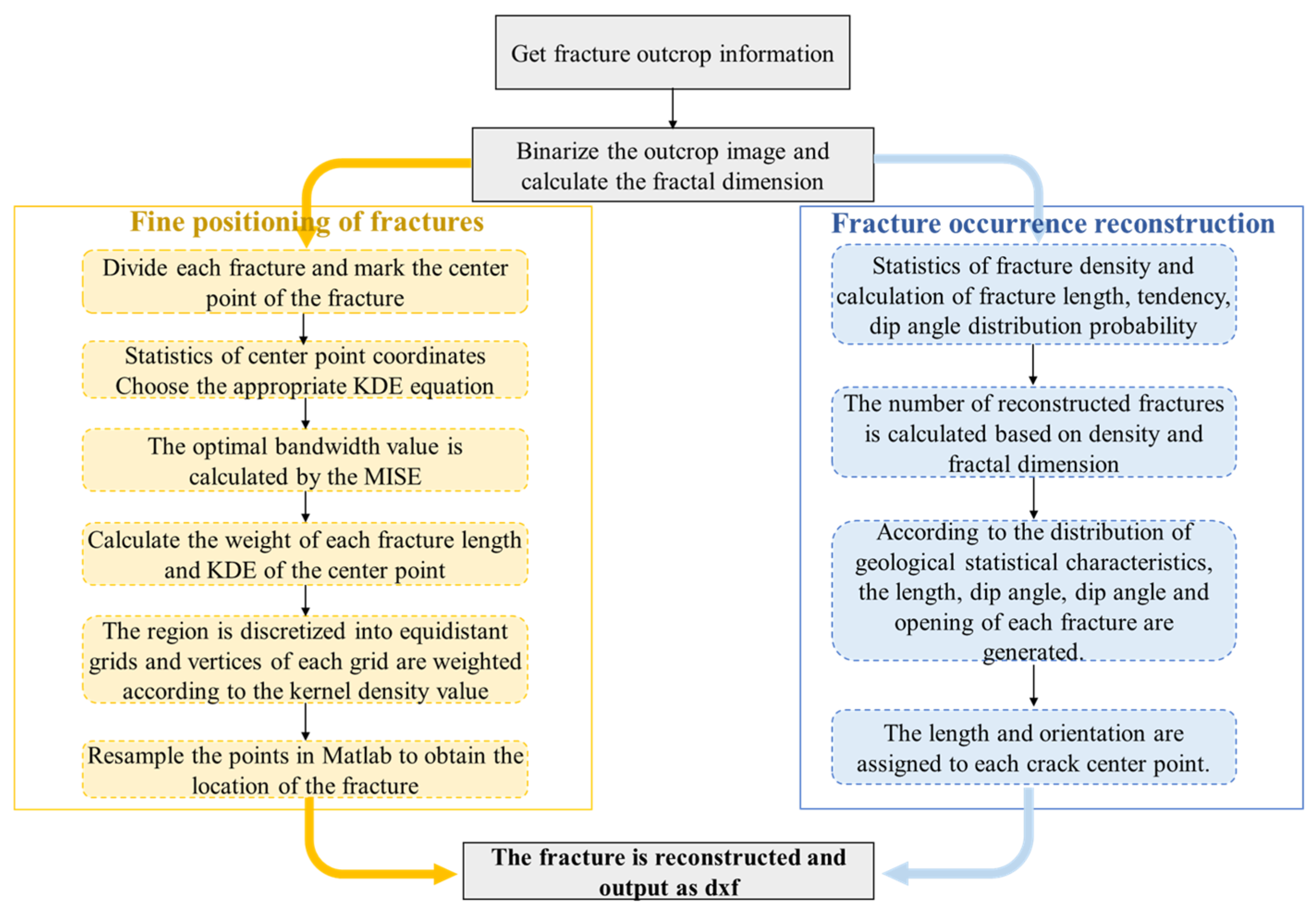
On the basis of this assumption, fracture-point sampling is performed in MATLAB 2024b by extending the sampling range to the entire study domain. The total number of sampled points is set equal to the number of fractures within the domain, and the generated points are regarded as the center points of the reconstructed fractures. Since these sampling points are generated from grid vertices, the spatial resolution of the reconstructed fracture positions is affected by grid spacing. Similar to the influence of bandwidth selection, a smaller and denser grid spacing provides a finer representation of the sampled points. Subsequently, the distributions of fracture length, orientation, and dip angle are generated in MATLAB using the Monte Carlo method. The sampled fracture positions are then randomly combined with the generated occurrence information to obtain the data required for fracture reconstruction. Finally, the reconstructed fracture field is generated in MATLAB and exported as a DXF file for subsequent finite element analysis. The overall procedure is presented in Figure 4.
Figure 4.
Flowchart of fracture-field reconstruction.
2.2. Fracture Field Reconstruction Results
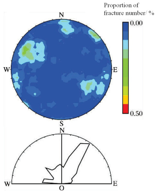
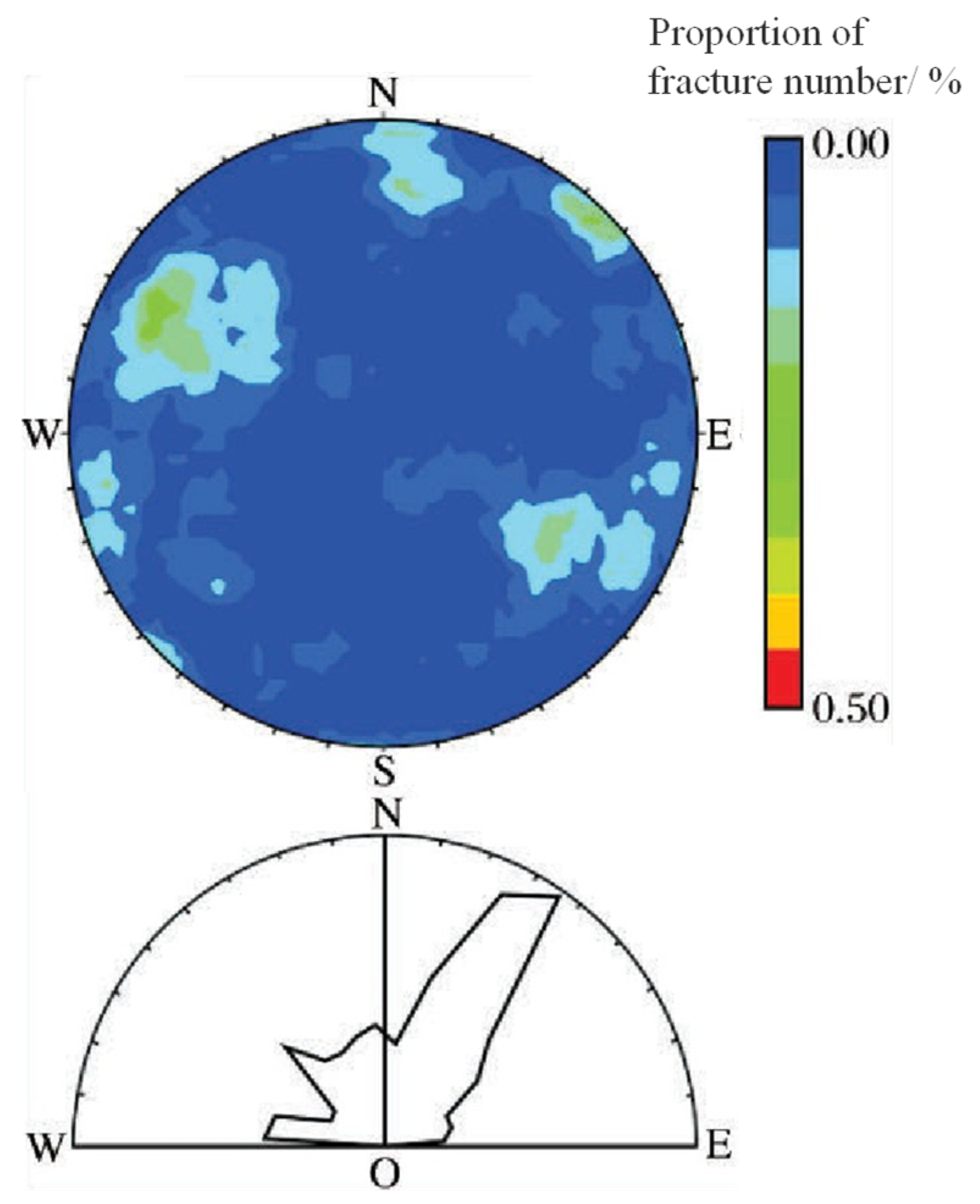
According to the statistical results, the mean fracture spacing in the study area is 0.5 m, and the fracture trace length follows a negative exponential distribution with a mean value of 8 m. Based on their orientations, the fractures are classified into three groups. The tendencies of the first and second groups follow lognormal distributions, with mean values of 120° and 297°, respectively. Because a large number of fractures have tendencies within the range of 0–20°, these fractures are treated separately as the third group, whose tendency follows a normal distribution with a mean value of 10°. The mean dip angles of the three fracture groups are 87°, 77°, and 77°, respectively. The corresponding geometric characteristics are presented in Figure 5 and Table 1 [28].
Figure 5.
Geometric characteristics of fractures in the Sanshandao mining area.
Table 1.
Statistical geometric characteristics of fractures in the study area.
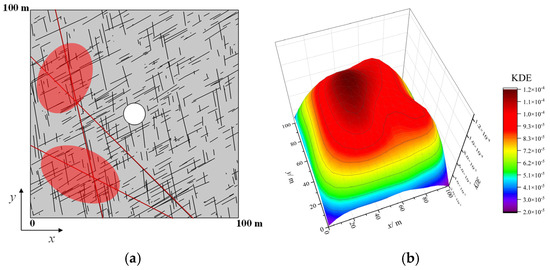
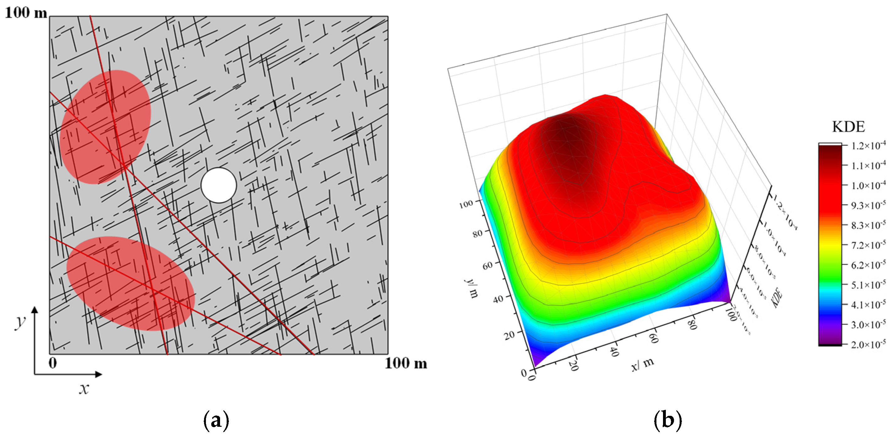
A domain of 100 m × 100 m was selected for fracture-field reconstruction, within which a total of 4330 fractures were generated. The reconstructed fracture field is presented in Figure 6a. In this figure, the red straight line denotes the major fault zone in the mining area, while the red region indicates an area with a relatively dense fracture distribution. The centroids of the generated fractures were subsequently extracted, and the corresponding kernel density distribution over the study domain is shown in Figure 6b. The results reveal several spatially clustered fracture zones, with fractures occurring more densely on the left side of the domain than on the right side. Compared with a reconstruction based on randomly distributed fractures, the reconstructed field is able to represent the concentration of fractures in the vicinity of the fault zone. However, it is worth mentioning that the model proposed in this study can describe the spatial intersection and connectivity between fracture sets in different directions, but it cannot strictly simulate the truncation and inheritance relationships in natural fracture networks. Moreover, the reconstruction model in this paper assumes that the parameters of fracture statistical information are independent of each other, and the influence of parameter correlation is not considered. In the follow-up study, the DFN model associated with the geometric characteristics of the fracture will be reconstructed.
Figure 6.
Reconstructed fracture field and spatial distribution of fractures: (a) Reconstructed fracture field; (b) Spatial distribution characteristics of fractures.
3. Results Multi-Field Coupling Mechanism of Underground Rock Mass
3.1. Coupled Model Equations
The deep metal mining area is characterized by the conditions commonly described as “three highs and one disturbance.” As shown by the geothermal profile in Figure 7, the formation temperature reaches 57 °C at a depth of 2000 m, indicating a pronounced high-temperature environment in the deep strata. Under these conditions, a coupled thermo–hydro–mechanical model is required to evaluate the effects of high in situ stress, high formation temperature, and elevated water pressure on the underground rock mass, thereby providing a basis for safe and efficient mining operations.
Figure 7.
Borehole temperature and geothermal gradient curves in the study area.
3.1.1. Mechanical Equations
Based on the differential equation of stress equilibrium, the geometric relationship, and the constitutive equation, the governing equation for the stress field in fractured rock masses is written as follows [32]:
where G is the shear modulus, Pa; K is the bulk modulus, Pa; E denotes Young’s modulus, Pa; ν is Poisson’s ratio; α represents the Biot coefficient; αT is the thermal expansion coefficient, m/°C; ε denotes strain; T is temperature, °C; and p is pore pressure, Pa.
The rock material is assumed to obey linear poroelastic behavior combined with an isotropic damage model [33]:
where σ′ denotes the effective stress, ω is the scalar damage variable, I represents the identity matrix, and D is the elastic stiffness matrix. In the adopted sign convention, compressive stress and strain are positive, whereas tensile stress and strain are negative.
The isotropic damage formulation is introduced to describe the failure process of the rock material. The damage variables under tensile and compressive conditions are represented by ωt and ωc, respectively. Under the assumption of elastic-brittle constitutive behavior, the damage evolution relationships are expressed as follows:
where κ is an internal variable recording the maximum equivalent strain attained during loading. The equivalent tensile and compressive strains are defined according to the smooth Rankine criterion. Here, εt0 = −ft0/E and εc0 = fc0/E denote the ultimate elastic tensile and compressive strains, respectively; ft0 and fc0 are the tensile and compressive strengths; ftr = ηft0 and fcr = ηfc0 are the corresponding residual strengths; η is the residual strength ratio; and κt and κc are the internal variables associated with tensile and compressive loading, respectively.
3.1.2. Normal Displacement and Shear Displacement of Fractures
For a natural fracture subjected to normal compressive loading, the variation in normal aperture is assumed to follow an exponential relationship:
where bn denotes the normal aperture, m; b0 and br are the initial and residual apertures, respectively, m; σ′n = σn − p represents the effective normal compressive stress; σn is the total normal stress; p is the pore pressure; ξ is the coefficient describing the relationship between stress and aperture, defined as 1/[Kn0(b0 − br)]; and Kn0 denotes the initial normal stiffness.
Accordingly, the response of a fracture under normal compression is characterized by a nonlinear normal stiffness, which is expressed as follows:
When both normal and shear deformations are considered, the fracture aperture bf is calculated by:
where ϕd represents the dilation angle, and ur denotes the residual shear displacement.
3.1.3. Fluid Flow in Fractured Porous Media
For single-phase fluid flow through fractured porous media, the mass conservation equation is expressed as follows [33]:
where ρw is the water density, kg/m3; φ denotes porosity, with φf and φm corresponding to the fracture and matrix porosities, respectively; t is time; U represents the fluid velocity; Q is the source term; and εv denotes the volumetric strain of the solid skeleton.
The movement of fluid within the medium is governed by Darcy’s law:
where k denotes permeability, with kf and km representing the permeabilities of the fractures and rock matrix, respectively; μw is the dynamic viscosity of water, Pa·s; and S is the storage coefficient, for which Sf and Sm refer to the values of the fractures and matrix, respectively.
For natural fractures, the permeability is related to fracture aperture according to the cubic law, and the corresponding storage coefficient is calculated as follows:
where cw is the compressibility of water. Since the natural fractures are assumed to contain no filling material, the fracture porosity φf is taken as 1.
The porosity of the rock matrix is calculated using:
where φ0 and φr are the initial and residual porosities, respectively; σ′ represents the effective mean stress; and ς is the coefficient describing the relationship between porosity and stress. For undamaged rock (ω = 0), this coefficient is expressed as cm/(φ0 − φr); for damaged rock (ω > 0), it is given by 1/[Kn(b0 − br)].
The permeability of the rock matrix is described by:
where k0 denotes the initial permeability of the matrix, and ζ is the coefficient relating damage to permeability. This coefficient is estimated according to the expression provided in Equation (13), in which h represents the width of the damaged zone and is approximately taken as the local element size in the numerical simulation.
The storage coefficient of the rock matrix is determined by:
where cm = 3(1 − 2ν)/E denotes the compressibility of the rock matrix.
3.1.4. Heat Transfer Equation
The heat exchange between the fluid and rock mass in discrete fractures is described using the heat-transfer formulation for porous media. The corresponding energy conservation equation is written as follows [34]:
where (ρCp)eff is the effective volumetric heat capacity, J/(m3·°C); Cw and λw denote the isobaric specific heat capacity and thermal conductivity of water, respectively; uf is the fluid velocity in the fractured reservoir, m/s; λeff represents the effective thermal conductivity, W/(m·°C); Cr is the isobaric specific heat capacity of the fractured reservoir, J/(kg·°C); and Qf,E denotes the heat exchange between the fluid and rock within the fractured reservoir, W/m3.
Heat conduction within the solid rock mass is governed by:
where Cs and λs are the isobaric specific heat capacity and thermal conductivity of the rock mass, respectively.
3.2. Model Validation
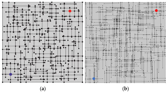
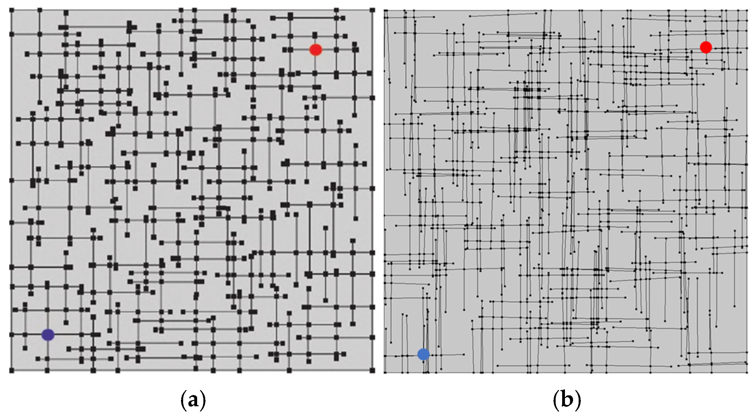
To evaluate the reliability of the proposed model, the simulation results were compared with those reported by He et al. [35]. In their study, a dual-medium thermo–hydro–mechanical coupling model was established to investigate the evolution of reservoir permeability during geothermal extraction. The computational configuration adopted for validation is shown in Figure 8. The hydraulically fractured hot dry rock reservoir is represented by a two-dimensional domain measuring 300 m × 300 m. The randomly generated fracture network mainly consists of two fracture sets. For each set, the fracture orientation follows a standard normal distribution, while the trace length is described by a normal distribution. The corresponding fracture-network parameters are listed in Table 2.
Figure 8.
Hot dry rock model containing a fracture network: (a) Model established by He et al. [35]; (b) Validation model.
Table 2.
Parameters of the fracture network used in the validation model.
A one-injection–one-production configuration is adopted in the model. As shown in Figure 8, the blue point represents the injection well, whereas the red point denotes the production well. The material parameters assigned to the fracture network are provided in the corresponding parameter Table 3. The initial water pressure in the reservoir is set to 40 MPa. Constant-pressure conditions are imposed at the wells, with pressures of 44 MPa and 40 MPa applied to the injection and production wells, respectively. Both wells have a diameter of 0.2 m, and all other boundaries are treated as no-flow boundaries. The initial temperature of both the reservoir rock and the contained water is 200 °C, while the injected water temperature is fixed at 20 °C. Thermal insulation is imposed along the outer boundaries of the model. For the stress-field simulation, displacement constraints are applied to the surrounding boundaries. In order to examine stress disturbance during the heat-extraction process more directly, the initial in situ stress is not included in this validation calculation.
Table 3.
Hot dry rock model parameters.
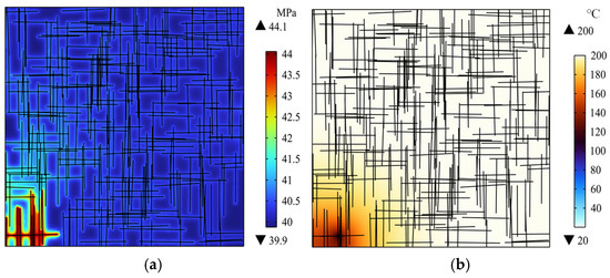
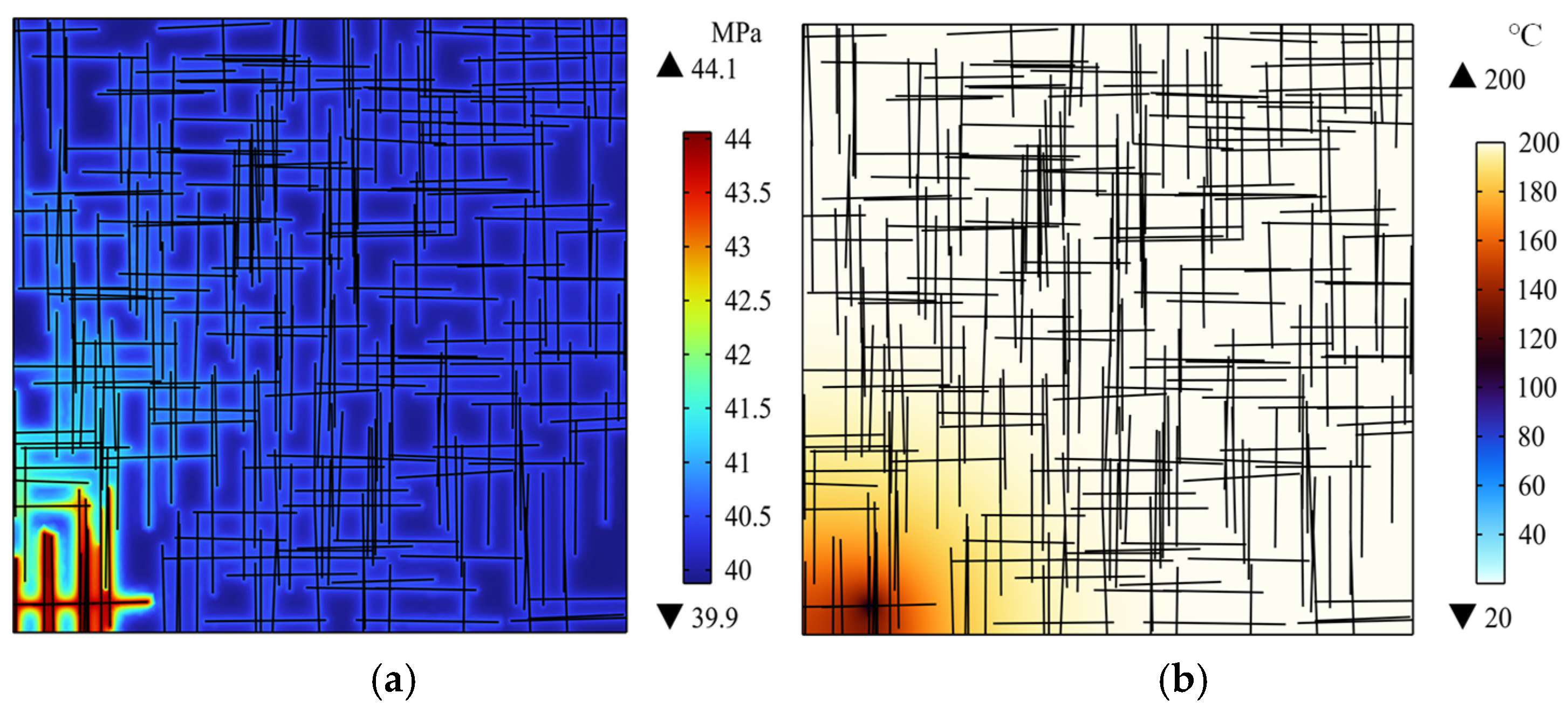
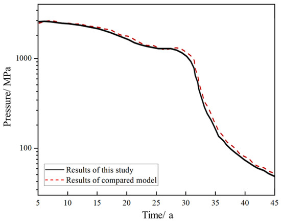
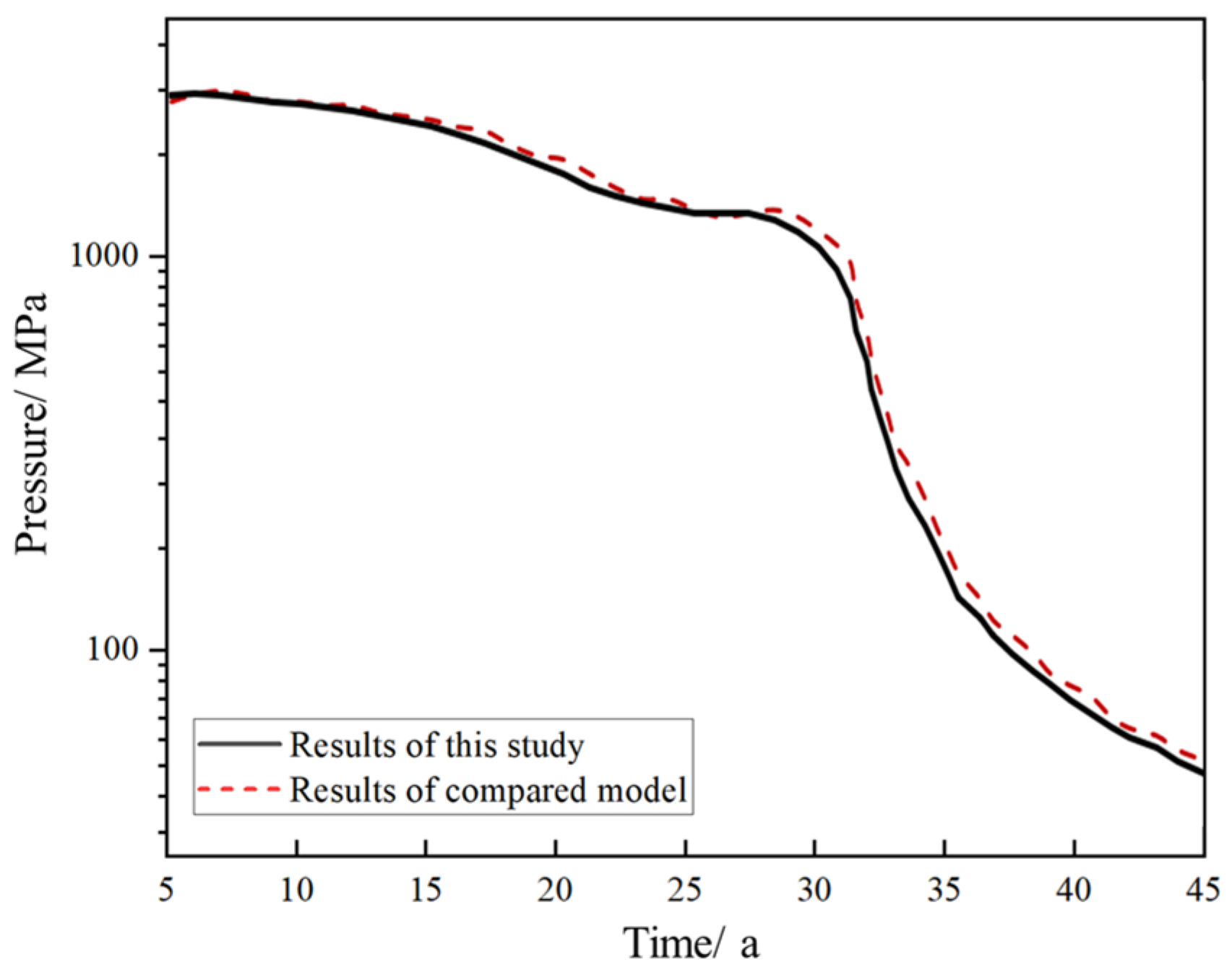
The calculated pressure and temperature distributions are presented in Figure 9. After 10 years of operation, the injection of high-pressure water causes the reservoir pressure to gradually increase. A limited amount of fluid enters the low-porosity and low-permeability rock matrix, whereas the principal flow pathways occur within fracture zones because of their higher permeability and greater flow velocity. Consequently, fluid flow within the reservoir exhibits a non-uniform distribution. Following the injection of low-temperature water into the hot reservoir, heat exchange between the cold fluid and the high-temperature rock mass also takes place mainly along the fracture zones. These results are consistent with those obtained by He et al. [35]. To further examine the reliability of the present model, the pressure evolution at the central point of the reservoir was monitored. The compared results were illustrated in Figure 10. The two sets of results exhibit a similar overall trend. A slightly lower value is obtained from the present model at 30 years, which is attributed in the original analysis to the randomness associated with the generated fracture network. Overall, the comparison supports the reliability of the established model. The verification of this study is mainly aimed at the rationality of numerical implementation, rather than the verification of on-site scale prediction ability. In the future, it is necessary to further check and verify the model parameters by combining the field monitoring data and the fracture normal-shear seepage test results.
Figure 9.
Pressure and temperature distributions in the hot dry rock reservoir: (a) Pressure; (b) Temperature.
Figure 10.
Pressure evolution at the central point of the hot dry rock reservoir.
3.3. Coupled Model and Results
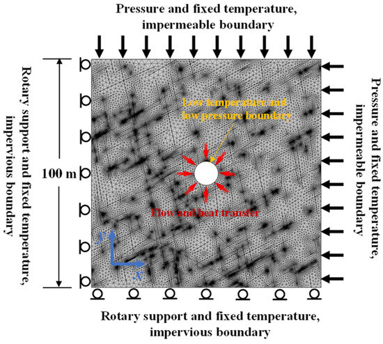
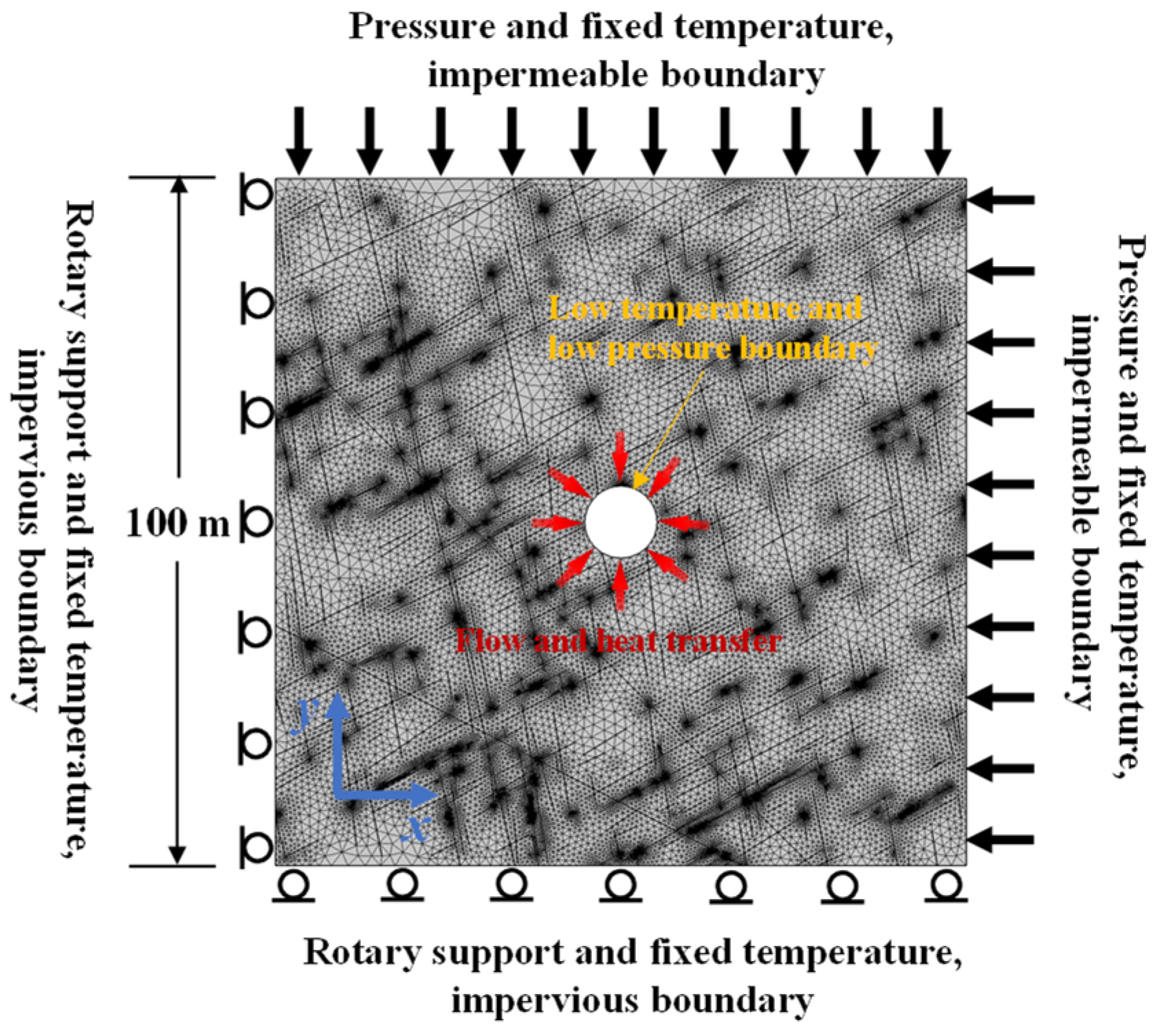
Using the reconstructed fracture field described above, a thermo–hydro–mechanical coupling model is established to investigate the behavior of fractured rock masses during shaft construction at a depth of 2000 m, as illustrated in Figure 11. The computational domain measures 100 m × 100 m, and a shaft with a diameter of 10.5 m is positioned at its center. Roller-support boundary conditions are imposed on the upper and right boundaries, whereas the original horizontal stresses of the formation are applied to the left and lower boundaries. According to the geological survey results, the maximum and minimum principal stresses at a depth of 2000 m are 70 MPa and 47 MPa, respectively.
Figure 11.
Boundary conditions of the thermo–hydro–mechanical coupling model for underground fractured rock masses.
The initial pore pressure of the formation is set to 20 MPa. The external boundaries are treated as impermeable, while atmospheric pressure is prescribed along the shaft boundary. For the temperature field, an initial temperature of 57 °C is assigned to the model, and the surrounding boundaries are maintained at 57 °C. The shaft boundary is set to room temperature, namely 10 °C, in order to examine temperature propagation within the fractured rock mass during shaft construction. The domain is discretized using triangular elements, resulting in a total of 82,723 elements with an average mesh quality of 0.82. The calculation is conducted using the built-in automatic highly nonlinear solver in COMSOL, with a calculation period of 50 days. The remaining material and fracture parameters are provided in Table 4.
Table 4.
Parameters of the multi-field coupling model.
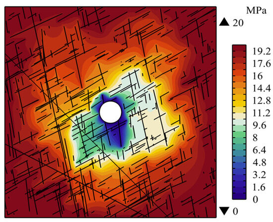
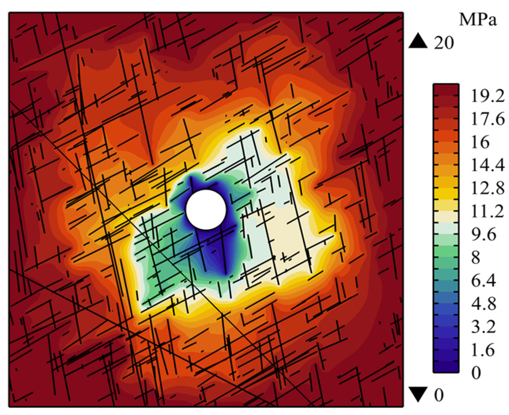
The pressure distribution obtained from the model is shown in Figure 12. Following the commencement of shaft construction, the high-pressure fluid initially stored in the formation flows toward the shaft through both the low-porosity and low-permeability rock matrix and the fractures. In the present model, the three fracture zones are concentrated in the lower-left region, where fractures are more densely distributed and exhibit stronger connectivity. Accordingly, the pressure in this region decreases more rapidly than that in other parts of the model. This region therefore constitutes the dominant seepage zone, and engineering protection against water inrush should give priority to this direction.
Figure 12.
Pressure distribution of the model.
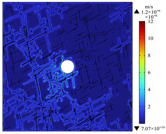
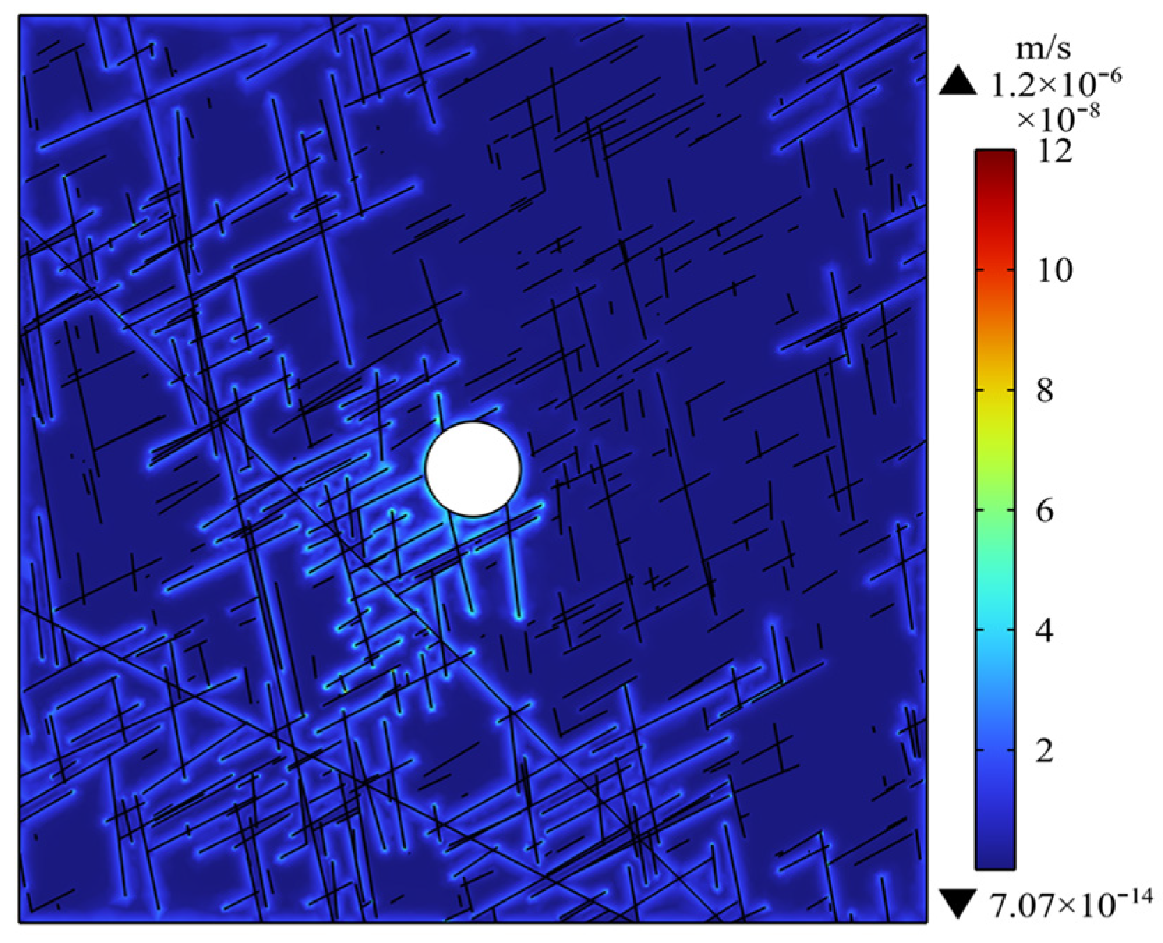
As indicated in Figure 13, the principal pathways of fluid migration are concentrated within the fracture zones, where permeability and flow velocity are relatively high and the pressure decreases earlier. The fluid velocity in the fractures is approximately three orders of magnitude greater than that in the rock matrix. Such rapid pressure reduction within the fractures consequently induces deformation of the surrounding rock matrix.
Figure 13.
Fluid velocity distribution at the initial stage.
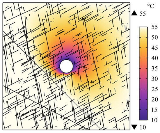
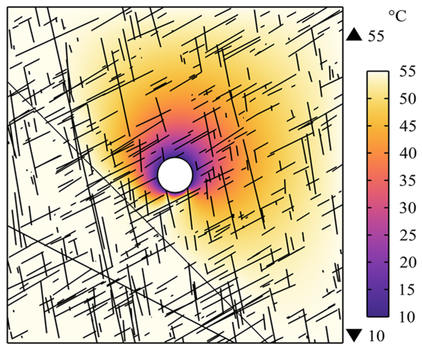
The temperature distribution of the model is presented in Figure 14. After shaft construction begins, the temperature in the surrounding region of the shaft becomes noticeably lower than the initial formation temperature, causing heat in the original formation to transfer toward the low-temperature zone. Only a small proportion of heat is transferred through the rock matrix because of its low porosity and low permeability, whereas most heat is transported with the fluid along fracture zones characterized by higher permeability and greater flow velocity. Consequently, the presence of fractures leads to an evidently non-uniform temperature distribution within the model. The current model is based on the assumption of local thermal equilibrium, and does not consider the possible thermal non-equilibrium effect between fracture and matrix. In the future, the bi-continuum LTNE model will be used to further analyze the heat transfer mechanism in the fracture network, so as to improve the accuracy of thermal–fluid–solid coupling simulation of deep fractured rock mass.
Figure 14.
Temperature transfer law of model.
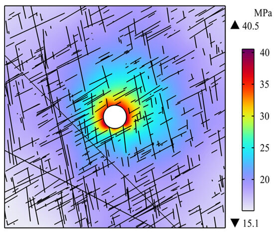
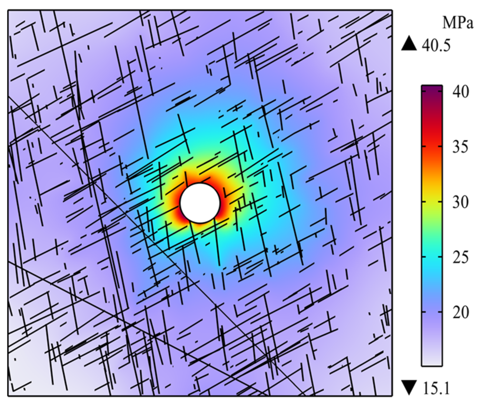
The stress distribution obtained from the model is shown in Figure 15. Owing to shaft construction, the Von Mises stress in the vicinity of the shaft is substantially higher than that in the remaining areas, with a maximum value of 122 MPa, approximately 1.7 times the original formation stress. In addition, the presence of fractures causes an uneven distribution of Von Mises stress within the formation. This phenomenon is related, on the one hand, to the differences in mechanical properties between fractures and the rock matrix, through which fractures affect the mechanical behavior of the rock mass. On the other hand, changes in the formation temperature field cause the high-temperature rock matrix to contract under cooling, thereby altering its mechanical state. Meanwhile, matrix deformation increases the fracture aperture and enhances the hydraulic conductivity of the formation. The resulting acceleration of temperature variation further contributes to redistribution of the stress field.
Figure 15.
The stress distribution of the model.
4. Discussion
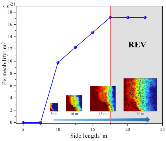
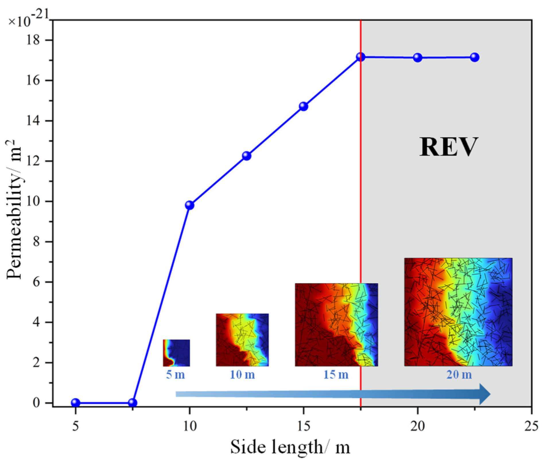
Fractures introduce heterogeneity into the physical and mechanical properties of underground rock masses. According to the concept of continuum mechanics, when the investigated rock-mass domain reaches a sufficiently large scale, the equivalent physical and mechanical properties of the fractured medium tend to stabilize at representative values. The corresponding characteristic scale is referred to as the representative elementary volume (REV) of the rock mass. To determine the REV of the fractured rock mass in the Sanshandao area, eight DFN submodels were extracted from the generated 100 m × 100 m fracture model. These submodels were centered at the coordinate point (50 m, 50 m), with the side length increasing from 5 m at an interval of 2.5 m.
For each submodel, a pressure of 10 MPa was imposed on the left boundary, atmospheric pressure was assigned to the right boundary, and the upper and lower boundaries were defined as impermeable. Figure 16 presents the variation in equivalent permeability with rock-mass size for the Sanshandao area. The equivalent permeability gradually increases as the model size becomes larger. When the side length reaches 17.5 m, the variation in permeability becomes very small, indicating that the fractured rock mass can be regarded as having reached its representative elementary volume at this scale.
Figure 16.
Equivalent permeability of fractured rock masses with different sizes in the Sanshandao area.
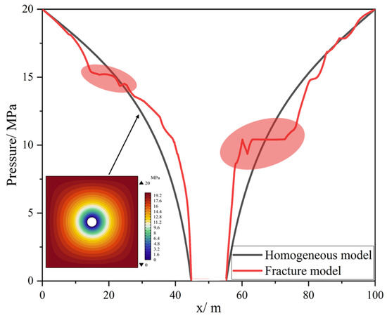
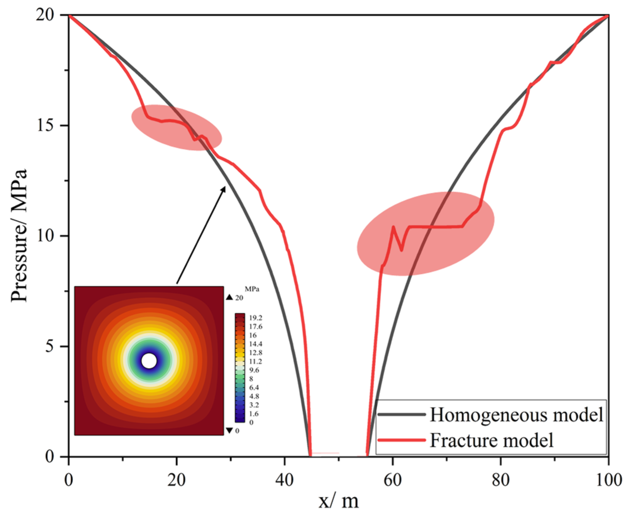
To further examine the influence of fractures on the hydraulic behavior of underground rock masses, a homogeneous model without fractures was constructed for comparison. The material parameters and boundary conditions were kept consistent with those adopted in the preceding analysis. Pressure variations along the section line at (y = 150) m were monitored for both the homogeneous model and the fractured model, and the comparison is shown in Figure 17. In the homogeneous model, the pressure decreases smoothly from 20 MPa at the external boundary to atmospheric pressure at the shaft boundary. By contrast, the pressure profile obtained from the fractured model presents distinct plateau-like and sawtooth-shaped variations. This difference indicates that hydraulic-head dissipation in fractured rock masses is spatially non-uniform. Therefore, the effects of fractures should be explicitly considered when evaluating the seepage characteristics of underground rock masses. However, the 17.5 m REV obtained in this paper should be regarded as a hydraulic REV in the strict sense, and its applicability to thermal and mechanical parameters needs to be further verified. Future research will use parameters such as equivalent elastic modulus and thermal conductivity to jointly determine the comprehensive REV under multi-field coupling conditions.
Figure 17.
Comparison of pressure variations along the (y = 150) m section line in the two models.
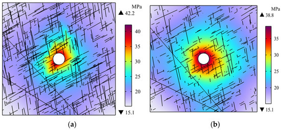
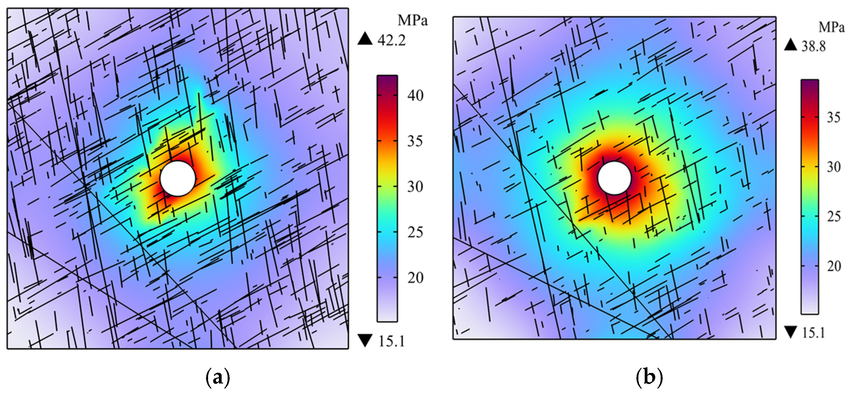
To investigate the effect of fracture length distribution on the mechanical response of underground rock masses, two additional fracture models were generated on the basis of the preceding model. Their mean fracture lengths were set to 6 m and 10 m, respectively, while the total number of fractures remained unchanged. The same boundary conditions as those applied to the model with a mean fracture length of 8 m were adopted for the comparative calculations. Figure 18 shows the stress distributions obtained for the models with different fracture-length characteristics. Following shaft construction, stress redistribution occurs in all three models, and the stress concentration around the shaft is substantially greater than the initial formation stress. Among these cases, the model with a mean fracture length of 10 m produces the highest Von Mises stress, reaching 129 MPa. This value is 11 MPa higher than that obtained for the model with a mean fracture length of 6 m. The difference is attributed to the larger proportion of the rock mass occupied by fractures when the average fracture length increases, which leads to higher permeability. Consequently, high-pressure formation water flows more rapidly toward the shaft, resulting in a sharper reduction in pore pressure around the shaft and a corresponding increase in the effective stress of the rock mass. Also, the increase in average fracture length not only increases the fracture volume fraction but also enhances the connectivity of fracture network, thus changing the pore pressure transfer path and stress redistribution mode.
Figure 18.
Stress distributions of models with different mean fracture lengths: (a) Average fracture length is 10 m; (b) Average fracture length is 6 m.
5. Conclusions
Based on extensive field-measured fracture data, this study represents fracture locations using their centroids and applies kernel density estimation (KDE) to describe the spatial distribution of fractures without assuming a predefined distribution form. Fourier convolution is then used to improve the efficiency of fracture-position reconstruction within the Discrete Fracture Network (DFN) model. The main conclusions are as follows:
- (1)
- The KDE-based method can identify the spatial distribution characteristics of fractures and represent the heterogeneity of fracture occurrence in the studied rock mass. In combination with Monte Carlo sampling, the fracture field of the underground rock mass was reconstructed in MATLAB, providing a basis for the subsequent numerical analysis.
- (2)
- A thermo–hydro–mechanical (THM) coupling model containing the reconstructed fracture network was developed in COMSOL. The numerical results show that fluid migration occurs primarily through the fractures, while heat transfer along fracture pathways is substantially faster than that through the surrounding rock matrix. Thus, fractures play an important role in the seepage and heat-transfer behavior of the investigated deep rock mass.
- (3)
- The fracture network has an evident influence on the stress distribution of the underground rock mass. Within the comparative models established in this study, an increase in mean fracture length leads to a stronger disturbance of the stress field. Therefore, the effects of fractures should be considered in numerical calculations and stability evaluations of deep fractured rock masses.
The model established in this study is based on the finite element method, and the characteristics of rough fracture filling, fracture slip and crack propagation are not considered. It is impossible to simulate the phenomenon of large-scale fracture reactivation and its induced topological structure evolution and crack directional propagation. In the following research, the phase-field method or continuous-discrete coupling method will be used to further study the problem. Moreover, the model in this paper does not consider the influence of seawater erosion for the time being, which is an important research direction. It will be studied in future research.
Author Contributions
Conceptualization, W.F.; Methodology, G.W.; Software, W.F.; Validation, W.F.; Investigation, Y.S.; Resources, Y.S.; Data curation, Y.S., L.Y. and Z.S.; Writing—original draft, G.W. and B.H.; Writing—review & editing, L.Y.; Visualization, B.H.; Supervision, B.H. and L.Y.; Project administration, Z.S.; Funding acquisition, G.W. and Z.S. All authors have read and agreed to the published version of the manuscript.
Funding
This research was funded by the Major Science and Technology Project of China Middling Coal (Grant: 20231BY001).
Data Availability Statement
Dataset available on request from the authors.
Acknowledgments
The authors are grateful for the financial support from the China Coal Construction Group Limited Corporation.
Conflicts of Interest
Authors Guoyuan Wang, Wenbo Fan, Yinhe Sun, Zhaoyang Song were employed by the company China Coal Construction Group Limited Corporation and Beijing China Coal Mine Engineering Company Limited. The remaining authors declare that the research was conducted in the absence of any commercial or financial relationships that could be construed as a potential conflict of interest.
Abbreviations
| KDE | Kernel density estimation |
| DFN | Discrete fracture network |
| THM | Thermo–hydro–mechanical |
| BEM | Boundary element method |
| FDM | Finite difference method |
| FEM | Finite element method |
| FVM | Finite volume method |
References
- Zhou, C.B.; Ye, Z.Y.; Yao, C.; Fan, X.C.; Xiong, F. Estimation of the anisotropy of hydraulic conductivity through 3D fracture networks using the directional geological entropy. Int. J. Min. Sci. Technol. 2024, 34, 137–148. [Google Scholar] [CrossRef] [Scilit]
- Wang, P.T.; Ma, C.; Zhang, B.; Gou, Q.; Tan, W.H.; Cai, M.F. Development of an improved three-dimensional rough discrete fracture network model: Method and application. Int. J. Min. Sci. Technol. 2023, 33, 1469–1485. [Google Scholar] [CrossRef] [Scilit]
- Sun, R.; Wang, J. Effects of in situ stress and multiborehole cluster on hydraulic fracturing of shale gas reservoir from multiscale perspective. J. Energy Eng. 2024, 150, 04024002. [Google Scholar] [CrossRef] [Scilit]
- Liu, R.C.; Huang, N.; Jiang, Y.J.; Jing, H.W.; Yu, L.Y. A numerical study of shear-induced evolutions of geometric and hydraulic properties of self-affine rough-walled rock fractures. Int. J. Rock Mech. Min. Sci. 2020, 127, 104211. [Google Scholar] [CrossRef] [Scilit]
- Mi, X.Z.; Yu, L.Y.; Zhang, J.; Liu, R.C.; Hu, B.W.; Wei, C. Study on the influence of statistical geometrical characteristics on the permeability tensor of fractured rock masses by the equivalent pipe network method. Comput. Geosci. 2024, 165, 105868. [Google Scholar] [CrossRef] [Scilit]
- Luo, L.; Liang, X.; Ma, B.; Zhou, H. A karst networks generation model based on the anisotropic Fast Marching algorithm. J. Hydrol. 2021, 600, 126507. [Google Scholar] [CrossRef] [Scilit]
- Zhang, J.; Liu, R.C.; Yu, L.Y.; Jing, H.W.; Yin, Q. Investigations on representative elementary volume and directional permeability of fractal-based fracture networks using polygon sub-models. Fractals 2020, 28, 2050085. [Google Scholar] [CrossRef] [Scilit]
- Xu, W.; Zhang, Y.; Li, X.; Wang, X.; Zhang, P. Study on three-dimensional fracture network connectivity path of rock mass and seepage characteristics based on equivalent pipe network. Environ. Earth Sci. 2019, 78, 516. [Google Scholar] [CrossRef] [Scilit]
- Song, S.; Xu, Q.; Chen, J.; Wang, F.; Liu, Y.; Liu, Y. Relationship between the representative element volume and discontinuity parameters. Q. J. Eng. Geol. Hydrogeol. 2021, 54, qjegh2019-071. [Google Scholar]
- Shakiba, M.; Lake, L.W.; Gale, J.F.W.; Laubach, S.E.; Pyrcz, M.J. Stochastic reconstruction of fracture network pattern using spatial point processes. Geoenergy Sci. Eng. 2024, 236, 212741. [Google Scholar] [CrossRef] [Scilit]
- Gottron, D.; Henk, A. Upscaling of fractured rock mass properties—An example comparing Discrete Fracture Network (DFN) modeling and empirical relations based on engineering rock mass classifications. Eng. Geol. 2021, 294, 106382. [Google Scholar] [CrossRef] [Scilit]
- Maillot, J.; Davy, P.; Le Goc, R.; Darcel, C.; Dreuzy, J.R. Connectivity, permeability, and channeling in randomly distributed and kinematically defined discrete fracture network models. Water Resour. Res. 2016, 52, 8526–8545. [Google Scholar] [CrossRef] [Scilit]
- Sun, R.; Wang, J.; Zhou, Y.; Shang, X.; Leung, C. Stability analysis of a compressed air energy storage cavern transformed from a horseshoe-shaped roadway in an abandoned coal mine. Deep Undergr. Sci. Eng. 2025, 4, 562–581. [Google Scholar] [CrossRef] [Scilit]
- Sun, R.; Wang, J.; Zhang, K.; Li, F.; Ding, X.; Guo, Q. Stress redistribution in a multilayer chamber for compressed air energy storage in abandoned coalmine: Elastic analytical insights and material choice. Energy Sci. Eng. 2023, 11, 4198–4223. [Google Scholar] [CrossRef] [Scilit]
- Steefel, C.; Appelo, C.; Arora, B.; Jacques, D.; Kalbacher, T.; Kolditz, O.; Lagneau, V.; Lichtner, P.C.; Mayer, K.U.; Meeussen, J.C.L.; et al. Reactive transport codes for subsurface environmental simulation. Comput. Geosci. 2015, 19, 445–478. [Google Scholar] [CrossRef] [Scilit]
- Vecchiarelli, A. Application of the 3-D Hydro-Mechanical Model Geofrac in Enhanced Geothermal Systems; Massachusetts Institute of Technology: New York, NY, USA, 2013. [Google Scholar]
- Abuaisha, M.; Eaton, D.; Priest, J.; Wong, R. Hydraulic Fracture Simulation Using the Geos Code; MINES Paris Tech: Paris, France, 2015. [Google Scholar]
- Clauser, C. Numerical Simulation of Reactive Flow in Hot Aquifers: Shemat and Processing Shemat; Springer Science & Business Media: Berlin, Germany, 2003. [Google Scholar]
- Rutqvist, J. Status of the tough-flac simulator and recent applications related to coupled fluid flow and crustal deformations. Comput. Geosci. 2011, 37, 739–750. [Google Scholar] [CrossRef] [Scilit]
- Kong, Y.; Pang, Z.; Shao, H.; Kolditz, O. Optimization of well-doublet placement in geothermal reservoirs using numerical simulation and economic analysis. Environ. Earth Sci. 2017, 76, 118. [Google Scholar] [CrossRef] [Scilit]
- Tong, F.; Jing, L.; Zimmerman, R. A fully coupled thermo-hydro-mechanical model for simulating multiphase flow, deformation and heat transfer in buffer material and rock masses. Int. J. Rock Mech. Min. Sci. 2010, 47, 205–217. [Google Scholar] [CrossRef] [Scilit]
- Pan, P.; Feng, X.; Huang, X.; Cui, Q.; Zhou, H. Coupled THM processes in EDZ of crystalline rocks using an elasto-plastic cellular automaton. Environ. Geol. 2009, 57, 1299–1311. [Google Scholar]
- Sun, Z.; Zhang, X.; Xu, Y.; Yao, J.; Wang, H.-X.; Lv, S.; Sun, Z.-L.; Huang, Y.; Cai, M.-Y.; Huang, X. Numerical simulation of the heat extraction in EGS with thermal-hydraulic-mechanical coupling method based on discrete fractures model. Energy 2017, 120, 20–33. [Google Scholar] [CrossRef] [Scilit]
- Yao, J.; Zhang, X.; Sun, Z.; Huang, Z.; Liu, J.; Li, Y.; Xin, Y.; Yan, X.; Liu, W. Numerical simulation of the heat extraction in 3D-EGS with thermal-hydraulicmechanical coupling method based on discrete fractures model. Geothermics 2018, 74, 19–34. [Google Scholar] [CrossRef] [Scilit]
- Hofmann, H.; Babadagli, T.; Yoon, J.; Blöcher, G.; Zimmermann, G. A hybrid discrete/finite element modeling study of complex hydraulic fracture development for enhanced geothermal systems (EGS) in granitic basements. Geothermics 2016, 64, 362–381. [Google Scholar] [CrossRef] [Scilit]
- Li, S.; Feng, X.G.; Zhang, D.; Tang, H. Coupled thermo-hydro-mechanical analysis of stimulation and production for fractured geothermal reservoirs. Appl. Energy 2019, 247, 40–59. [Google Scholar] [CrossRef] [Scilit]
- Sun, R.; Zhao, W.; Wang, L.; Song, Q.; Yu, X.; Pang, S.; Zhang, L. Data-driven multiscale modeling of crack evolution in compressed energetic composites. Int. J. Mech. Sci. 2025, 309, 111043. [Google Scholar] [CrossRef] [Scilit]
- Liu, G.; Ma, F.; Zhao, H.; Guo, J.; Hou, C.; Li, W. Fracture Distribution Law and 3D Modeling of Main Permeable Roadways in Xishan Mining Area of Sanshandao Gold Mine. Gold Sci. Technol. 2019, 27, 199–206. (In Chinese) [Google Scholar]
- Mi, X.; Yu, L.; Zhang, J.; Liu, R.; Hu, B.; Qiu, S. Analysis of fracture spatial distributions and fast reconstruction of discrete fracture networks model based on non-parametric kernel density estimation method. Eng. Geol. 2025, 351, 108034. [Google Scholar] [CrossRef] [Scilit]
- Wang, Y.; Ding, Y.; Shahrampour, S. TAKDE: Temporal Adaptive Kernel Density Estimator for Real-Time Dynamic Density Estimation. IEEE Trans. Pattern Anal. Mach. Intell. 2023, 45, 13831–13843. [Google Scholar] [CrossRef] [Scilit] [PubMed]
- Miecznikowski, J.; Wang, D.; Hutson, A. Bootstrap MISE Estimators to Obtain Bandwidth for Kernel Density Estimation. Commun. Stat.-Simul. Comput. 2010, 39, 1455–1469. [Google Scholar] [CrossRef] [Scilit]
- Mi, X.; Yu, L.; Hu, B.; Su, H.; Shi, M.; Li, Y. Gas transport characteristics and airtightness evaluation of lined rock cavern for compressed air energy storages (caes). Energy 2025, 337, 138738. [Google Scholar] [CrossRef] [Scilit]
- Lei, Q.; Doonechaly, N.; Tsang, C. Modelling fluid injection-induced fracture activation, damage growth, seismicity occurrence and connectivity change in naturally fractured rocks. Int. J. Rock Mech. Min. Sci. 2021, 138, 104598. [Google Scholar] [CrossRef] [Scilit]
- Zhang, Y.; Li, Y.; Zheng, H.; Fan, B. A Novel Fully Coupled Thermo-Hydro-Mechanical-Damage Model for Hydraulic Fracture Propagation in Fractured Geothermal Reservoirs. Comput. Geotech. 2025, 185, 107364. [Google Scholar] [CrossRef] [Scilit]
- He, S.; Li, C.; Sun, K. Effects of permeability evolution on EGS hot mining performance. Chin. J. Appl. Mech. 2024, 41, 938–947. [Google Scholar]

Disclaimer/Publisher’s Note: The statements, opinions and data contained in all publications are solely those of the individual author(s) and contributor(s) and not of MDPI and/or the editor(s). MDPI and/or the editor(s) disclaim responsibility for any injury to people or property resulting from any ideas, methods, instructions or products referred to in the content. |
© 2026 by the authors. Licensee MDPI, Basel, Switzerland. This article is an open access article distributed under the terms and conditions of the Creative Commons Attribution (CC BY) license.