Research on the Application of the Joint Algorithm of Improved Wavelet Denoising and Improved UKF in Radar Measurement Data Processing

Abstract

To address the insufficient parameter estimation accuracy and poor filtering convergence caused by noise in radar trajectory measurement data, this paper proposes a joint framework combining SW-STPSO adaptive wavelet denoising and an improved Unscented Kalman Filter (UKF). First, SW-STPSO preprocesses noisy data using a sliding-window strategy and improved particle swarm optimization to adapt wavelet parameters to local noise characteristics. Then, the improved UKF adopts exponential-decay adaptive Q adjustment and covariance matrix positive-definite regularization to achieve high-precision estimation of ballistic parameters, including position, velocity, and ballistic coefficient. Simulation results show that: (1) SW-STPSO denoising improves subsequent parameter-estimation accuracy by more than 60% compared with the case without denoising; (2) the improved UKF achieves 37% faster convergence and 42% higher stability than the traditional UKF; and (3) the joint scheme reduces the position RMSE, velocity RMSE, and ballistic-coefficient RMSE to 0.92 m, 0.256 m/s, and 0.023 m²/kg, respectively. These results indicate that the proposed method is effective for radar trajectory data processing under the adopted simulation conditions.

1. Introduction

In precision guidance and strike systems, the high-precision identification of radar ballistic parameters is critical for ballistic correction and impact point prediction [1]. Radar measurement is inevitably affected by noise, and the strong nonlinearity of ballistic systems leaves traditional parameter identification methods with insufficient accuracy and poor robustness, which fail to meet complex engineering requirements [2,3].

To address the challenges of nonlinearity and noise suppression in ballistic parameter identification, numerous studies have been conducted in recent years. The Kalman filter series of algorithms have become the mainstream technology for ballistic data processing due to their excellent state estimation performance [4,5]. The Extended Kalman Filter (EKF) uses linearization to handle nonlinear models; however, it tends to introduce significant errors in highly nonlinear scenarios, thereby impairing parameter estimation accuracy [6]. The Unscented Kalman Filter (UKF) avoids the computation of the Jacobian matrix by using the Unscented Transform (UT), thereby improving the estimation accuracy of nonlinear systems [7,8]. To further improve UKF performance, a variety of enhancement strategies have been reported in the literature: Xie Kai et al. [9] constructed an inverse UKF algorithm with a seven-dimensional state vector, which breaks through the limitation of the traditional six-dimensional model that ignores core aerodynamic parameters and improves the accuracy of ballistic extrapolation; Afrasiabi et al. [10] proposed a hybrid method combining AI-aided Kalman filtering, discrete wavelet transform, and genetic algorithm; and Ge Yutong et al. [11] proposed an improved Kalman filtering algorithm based on Quantum Particle Swarm Optimization (QPSO), addressing noise and clutter interference in Ground-Penetrating Radar (GPR) data interpretation.

In a broader context, recent studies on radar–communication integrated systems have also shown that joint optimization of sensing and communication resources is important for improving overall system performance. For example, integrated power, bandwidth, and subchannel allocation has been investigated in RCC and UAV-assisted DFRC networks, and joint resource–trajectory optimization has also been reported for UAV-enabled DFRC systems [12,13,14]. Although these studies focus on resource allocation rather than radar trajectory data denoising and parameter estimation, they demonstrate the growing importance of coordinated optimization in advanced radar-related systems.

In terms of noise suppression, wavelet analysis has become an effective method for denoising radar measurement data due to its advantage of multiscale decomposition [15]. Yang Zhaozhe et al. [16] combined wavelet filtering with UKF, and suppressed the interference of measurement noise on filtering results through preprocessing; Subin Koshy et al. [17] proposed a dynamic state estimation method for power systems that combines wavelet transform with an improved Unscented Kalman Filter; and Tao Zhang et al. [18] proposed a capacitance state monitoring strategy integrating Haar wavelet transform and Kalman filtering.

Despite certain progress being achieved in existing research, there remain problems that urgently need to be addressed: first, the traditional UKF adopts a fixed process noise covariance matrix Q, which tends to lead to severe oscillations and slow convergence in the initial stage of iteration; second, a single denoising or filtering strategy finds it difficult to balance noise suppression and feature preservation, resulting in large parameter estimation errors in the strong noise environment of radar; and third, some improved algorithms focus on the optimization of a single performance index and fail to realize the coordinated improvement of accuracy, convergence speed and robustness.

To address these gaps, this paper proposes a joint framework combining SW-STPSO adaptive wavelet denoising and an improved UKF for radar trajectory data processing. In the present study, because real radar measurement data are not available, the radar measurement data used in the simulations are constructed by adding Gaussian noise to ideal ballistic trajectory data. Accordingly, the proposed method is evaluated from three aspects: estimation accuracy, convergence behavior, and filtering stability under the adopted noisy measurement conditions. Estimation accuracy is quantified by the RMSE and maximum absolute error (MaxAE) of the identified position, velocity, and ballistic coefficient. Convergence behavior is assessed by the oscillation and convergence characteristics of the ballistic-coefficient estimate during the initial iteration stage. Filtering stability is discussed mainly in terms of the continuity of the estimation process under the adopted noisy conditions and whether covariance degeneration leads to filter interruption, rather than in terms of explicit resistance to anomalous measurement outliers. Specifically, wavelet parameters are optimized to enhance the adaptability of denoising to local noise characteristics, while the improved UKF is designed to alleviate ballistic-coefficient oscillation, slow convergence, and filtering interruption. Simulation experiments are carried out to evaluate the effectiveness of the proposed method.

2. Model

The aerodynamic motion of projectiles is affected by the coupling of multiple factors. Although the six-degree-of-freedom (6-DOF) ballistic model can fully characterize the dynamic characteristics of projectiles, it has the limitations of high parameter dependence and huge computational complexity. Moreover, key parameters such as roll angular velocity required by the model cannot be obtained from radar measurement data, making it difficult to apply directly. In contrast, the four-degree-of-freedom (4-DOF) ballistic model still relies on roll-related aerodynamic parameters to characterize lateral forces; thus, it is also limited by the dimensional deficiency of radar measurement data and cannot be effectively implemented. Based on this, to adapt to the characteristics of measured radar data and balance ballistic accuracy with computational efficiency, this study adopts a three-degree-of-freedom (3-DOF) ballistic model for simulation analysis. Although this model does not consider certain aerodynamic effects such as projectile roll and lift force, it can significantly reduce the computation time while ensuring that the modeling accuracy meets the requirements of engineering applications, by combining the measurable dimensions of radar data and the practical needs of error compensation, thus achieving an optimal balance between accuracy and efficiency [19].

$$\left\{\begin{array}{cc}\hfill {\displaystyle \frac{\mathrm{d}{v}_x}{\mathrm{d}t}}& =-C{\displaystyle \frac{\rho v^2}{2m}}S{c}_{x0}cos{\theta }_{a}cos{\psi }_2\hfill \\ \hfill {\displaystyle \frac{\mathrm{d}{v}_y}{\mathrm{d}t}}& =-C{\displaystyle \frac{\rho v^2}{2m}}S{c}_{x0}sin{\theta }_{a}cos{\psi }_2-g\hfill \\ \hfill {\displaystyle \frac{\mathrm{d}{v}_z}{\mathrm{d}t}}& =-C{\displaystyle \frac{\rho v^2}{2m}}S{c}_{x0}sin{\psi }_2\hfill \\ \hfill {\displaystyle \frac{\mathrm{d}x}{\mathrm{d}t}}& =v_x\hfill \\ \hfill {\displaystyle \frac{\mathrm{d}y}{\mathrm{d}t}}& =v_y\hfill \\ \hfill {\displaystyle \frac{\mathrm{d}z}{\mathrm{d}t}}& =v_z\hfill \\ \hfill {\displaystyle \frac{\mathrm{d}C}{\mathrm{d}t}}& =0\hfill \end{array}\right.$$

(1)

$$\left\{\begin{array}{cc}\hfill v& =\sqrt{v_x^2+v_y^2+v_z^2}\hfill \\ \hfill S& =\pi ·D^2/4\hfill \\ \hfill {\theta }_a& =arctan\left({\displaystyle \frac{v_y}{v_x}}\right)\hfill \\ \hfill {\psi }_2& =arctan\left({\displaystyle \frac{v_z}{v_x}}\right)\hfill \end{array}\right.$$

(2)

where $v_x$, $v_{\mathrm{y}}$, $v_z$ and x, y, z refer to the velocity components and position components in the ground three-axis coordinate system, respectively; C refers to the ballistic coefficient; v refers to the combined velocity of the projectile, ${\theta }_a$ refers to the ballistic inclination, ${\psi }_2$ refers to the ballistic declination, $\rho$ refers to the density, m refers to the mass of the projectile, S refers to the cross-sectional area of the projectile, D refers to the diameter of the projectile, $c_{x0}$ refers to the coefficient of resistance, and g refers to the acceleration of gravity.

To further assess the influence of model simplification within the application scope of this study, an extended uncontrolled ballistic comparison was conducted between the 3-DOF and 6-DOF models under five representative short-time initial conditions. The comparison includes the position deviation at $t=6$ s, the same-range deviation in the y-z plane at $x=2200$ m, and the maximum trajectory deviation over the interval from 0 to 6 s. The results are summarized in Table 1.

Table 1. Extended comparison between the 3-DOF and 6-DOF models under five representative short-time uncontrolled cases.

Case	Initial Speed (m/s)	Launch Angle (deg)	Deviation at $\mathit{t}=6$ s (m)	Same-Range Deviation in the $\mathit{y}\mathbf{\text{-}}\mathit{z}$ Planeat $\mathit{x}=2200$ m (m)	Maximum Deviation over 0–6 s (m)
Case 1	950	45	0.204627	0.243331	0.204627
Case 2	900	45	0.206019	0.280293	0.206019
Case 3	1000	45	0.204003	0.212101	0.204003
Case 4	950	40	0.217966	0.188563	0.217966
Case 5	950	50	0.190319	0.331669	0.190319

As shown in Table 1, the deviation between the 3-DOF and 6-DOF models remains limited under all five representative short-time uncontrolled cases. The position deviation at $t=6$ s stays within approximately 0.19–0.22 m, while the same-range deviation in the y-z plane at $x=2200$ m remains within approximately 0.19–0.33 m. These results suggest that, for the short-time uncontrolled ballistic conditions of interest here, the 3-DOF model provides an acceptable approximation to the 6-DOF model while maintaining substantially lower model complexity.

However, this conclusion should be understood within the scope of the representative short-time uncontrolled cases examined here, rather than as evidence that the 3-DOF model can universally replace the 6-DOF model in all flight scenarios, disturbance environments, or long-duration ballistic conditions.

3. Design of the Improved Wavelet Transform Algorithm

Wavelet transform, thanks to its excellent time-frequency localization characteristics, has become a preferred technology for the preprocessing of noisy non-stationary radar trajectory data. It can synchronously capture both the low-frequency core features and high-frequency details of the signal, which matches the data characteristic of being globally non-stationary but locally approximately stationary, thus making up for the limitation of the Fourier transform in global frequency analysis. By separating signals from noise through multiscale decomposition, it suppresses Gaussian white noise in a targeted manner, satisfying the temporal consistency requirements for subsequent Kalman filtering [20].

3.1. Principle of the Traditional Particle Swarm Optimization Algorithm (PSO)

The Particle Swarm Optimization (PSO) algorithm is a swarm-intelligence optimization method that was first proposed in 1995 and has since been widely applied in various optimization fields.Within the PSO optimization framework, each particle corresponds to a potential solution in the search space, and its performance is quantitatively evaluated by a predefined fitness function. In this study, the fitness function is defined as the Root Mean Square Error (RMSE) between the denoised signal and the corresponding reference signal, so that the optimization process directly targets the reduction of denoising error. Therefore, the particle search is guided toward parameter combinations that simultaneously preserve the underlying trajectory characteristics and suppress measurement noise. By iteratively updating the position and velocity vectors of particles, the algorithm leverages the information sharing and collaborative search mechanisms among particles to guide the entire swarm to gradually approach the optimal solution region, and eventually converges to the global optimal solution or an approximate optimal solution that meets engineering requirements [21].

3.2. Principle of the Harris Hawks Optimization Algorithm (HHO)

The Harris Hawks Optimization (HHO) algorithm is a novel swarm intelligence optimization algorithm inspired by the predatory behaviors of Harris hawks in nature. By simulating the complete predation process of hawk swarms—searching for prey, surrounding prey, and attacking prey—it achieves efficient global optimization in complex parameter spaces [22]. This algorithm does not rely on gradient information and performs optimization through iterative position updates and fitness evaluation of population individuals. The key logic and parameter definitions of HHO are as follows:

• Population Initialization. The algorithm first randomly generates N “hawk swarm individuals” within the preset parameter search space, and the position vector of each individual corresponds to a set of parameters to be optimized (wavelet basis, decomposition level, and reconstruction level). The initialization formula is as follows:

  $$X_{i,j}=l{b}_j+r\times (u{b}_j-l{b}_j)$$

  (3)

  where $X_{i,j}$ denotes the position of the i-th hawk in the j-th dimension parameter, $l{b}_j$ and $u{b}_j$ represent the lower bound and upper bound of the j-th dimension parameter, respectively, and r is a random number uniformly distributed within the interval $[0,1]$. In this study, the population size $N=25$ (number of hawks) and the parameter dimension $dim=3$. This formula ensures that the initial population is uniformly distributed within the parameter space, covering all potential optimal solution regions.
• Energy Factor Design. HHO regulates the behavioral switching of hawk swarms by means of “rabbit energy” (prey energy). The core energy factors include the energy attenuation factor $E_1$, random energy $E_0$, and escape energy $E_2$, whose expressions are given as follows:

  $$E_1=2\times (1-t/T)$$

  (4)

  $$E_0=2\times r-1$$

  (5)

  $$E_2=E_1\times E_0$$

  (6)

  where t is the current iteration number, and T is the maximum iteration number. The algorithm is in the exploration phase when $E_1\ge 1.3$, and in the exploitation phase when $E_1<1.3$.
• Exploration Phase. When $E_1\ge 1.3$, the algorithm enters the exploration phase. The objective of this phase is to enable the hawk swarm to search for prey (optimal parameter combination) in a global scope, and position update is realized through two random strategies to avoid falling into a local optimum:
  • Random Disturbance Search Strategy: Randomly select the position of another hawk as the reference, and realize position update through random sign disturbance, to simulate the dispersed search behavior of the hawk swarm. Its expression is given as follows:

    $$X(t+1)=Xrand\pm C_1\times \left|Xrand-2\times r\times X\left(t\right)\right|$$

    (7)

    where $Xrand$ is the position of the randomly selected reference hawk, and $C_1$ is a constant with a value of 0.1.
  • Global Optimum-Guided Search Strategy: With the current global optimal solution as the center, position update is achieved through population mean disturbance, to simulate the behavior of hawk swarms gathering toward potential prey areas. Its expression is given as follows:

    $$X(t+1)=XRabbit\pm C_2\times \left(XRabbit-Xmean\right)$$

    (8)

    where $XRabbit$ is the position of the optimal hawk, $Xmean$ is the mean position of the current hawk swarm, and $C_2$ is a constant with a value of 2.
• Exploitation Phase. When $E_1<1.3$, the algorithm enters the exploitation phase. The objective of this phase is to achieve precise convergence within the potential optimal regions identified in the exploration phase. Four attack strategies are adopted to simulate the collaborative predation behaviors of Harris hawks, to improve the accuracy of local search:
  • Hard Siege Strategy (when $r\ge 0.4$ and $\left|E_2\right|<0.5$): When the prey energy is low, and its escape ability is weak, the hawk swarm directly approaches the prey, and the position update formula is as follows:

    $$X(t+1)=XRabbit\pm C_3\times E_2\times \left|XRabbit-X\left(t\right)\right|$$

    (9)

    where $C_3$ is a constant with a value of 0.05.
  • Soft Siege Strategy (when $r\ge 0.4$ and $\left|E_2\right|\ge 0.5$): When the prey energy is high, and it still has escape ability, the hawk swarm adjusts the attack rhythm through random jump intensity, and the formula is as follows:

    $$X(t+1)=XRabbit\pm C_3\times E_2\times 2\times (1-r)\times \left|XRabbit-X\left(t\right)\right|$$

    (10)
  • Soft Siege Strategy with Asymptotic Dive (when $r<0.4$ and $\left|E_2\right|\ge 0.5$): Some hawks dive directly to attack, while others flank the prey from behind via Levy flight to prevent the prey from escaping. The position update requires comparing the fitness of the two attack modes and selecting the better position. The position update formula is as follows:

    $$X_1(t+1)=XRabbit\pm C_4\times E_2\times 2\times (1-r)\times \left|XRabbit-X\left(t\right)\right|$$

    (11)

    $$X_2(t+1)=XRabbit-E_2\times \left|2\times (1-r)\times XRabbit-X\left(t\right)\right|+\mathrm{rand}(1,dim)·\mathrm{levy}\_\mathrm{value}$$

    (12)

    where $C_4$ is a constant with a value of 0.01, and $\mathrm{levy}\_\mathrm{value}$ denotes the random step size of the Levy flight generated in accordance with the Levy distribution. The formula is expressed as:

    $$\mathrm{levy}\_\mathrm{value}=u/{\left|v\right|}^{1/\beta }$$

    (13)

    where $\beta =1.5$, and both u and v follow the standard normal distribution.
  • Hard Siege Strategy with Asymptotic Dive (where $r<0.4$ and $\left|E_2\right|<0.5$): When the prey energy is extremely low, the hawk swarm coordinately dives around the population mean. Disturbance generated by Levy flight is adopted to avoid falling into a local optimum, thereby further improving the convergence accuracy. The position update formula is as follows:

    $$X_1(t+1)=XRabbit-C_4\times E_2\times 2\times (1-r)\times \left|XRabbit-Xmean\right|$$

    (14)

    $$X_2(t+1)=XRabbit-E_2\times \left|2\times (1-r)\times XRabbit-Xmean\right|+\mathrm{rand}(1,dim)·\mathrm{levy}\_\mathrm{value}$$

    (15)
• Boundary Checking and Fitness Evaluation. After each position update, the positions of individuals that exceed the parameter range are corrected to ensure all parameters fall within a reasonable range. Subsequently, the fitness of each individual in the hawk swarm is calculated, and the global optimal solution $XRabbit$ is updated.

3.3. Basic Principles of Wavelet Transform

Wavelet transform is a time-frequency analysis method based on multiresolution analysis, whose core advantage lies in its ability to perform localized analysis of non-stationary signals via a wavelet basis with adjustable scales [23,24]. It not only retains the abrupt change characteristics of signals in the time domain, but also accurately captures the frequency distribution patterns in the frequency domain. Therefore, it has been widely applied to the denoising tasks of non-stationary signals in fields such as radar and communications. The expression of the continuous wavelet transform is as follows:

$$\mathrm{CWT}(a,b)={\displaystyle \frac{1}{\sqrt{a}}}{\int }_{-\infty }^{+\infty }f\left(t\right)·\psi \left({\displaystyle \frac{t-b}{a}}\right)dt$$

(16)

where a is the scale factor (controlling the dilation and contraction of the wavelet basis, corresponding to the frequency-domain resolution: the smaller the value of a, the narrower the wavelet basis, resulting in higher time-domain resolution and lower frequency-domain resolution; the opposite is true when a is larger); b is the translation factor (controlling the position of the wavelet basis in the time domain, corresponding to time-domain localization); $\psi \left(t\right)$ is the mother wavelet (e.g., db4, sym8, haar, etc., which must satisfy the admissibility condition); and $f\left(t\right)$ is the non-stationary signal to be analyzed.

In engineering practice, the signals actually processed are discrete sampled signals, so the Discrete Wavelet Transform is the core form of application. In this paper, the MATLAB R2022b Wavelet Transform Toolbox is adopted to implement core functions (such as ‘wavedec’ for decomposition and ‘wrcoef’ for reconstruction).

3.4. Adaptive Wavelet Transform Denoising Algorithm Based on Improved Particle Swarm Optimization (SW-STPSO)

The standard PSO algorithm is widely used for function optimization but suffers from drawbacks such as easy convergence to local optima and redundant iterations. To address these issues, this paper modifies the algorithm to form STPSO (Improved Particle Swarm Optimization) and further integrates a sliding window strategy to propose the SW-STPSO adaptive wavelet denoising algorithm, enhancing adaptability to local noise characteristics of radar data.

3.4.1. Sobol Sequence Initialization

The quality of the initial population distribution is an important factor affecting the convergence behavior and optimization performance of population-based optimization algorithms. In high-dimensional search spaces, conventional random initialization may lead to uneven population coverage, which can restrict the early-stage exploration ability of the optimizer. For this reason, this study adopts the Sobol sequence [25] for population initialization. As a low-discrepancy sequence, it generates relatively uniform sample points in the solution space through deterministic mathematical construction, which is beneficial for improving the coverage of the initial population when the number of particles is limited.

As shown in Table 2, Sobol-sequence initialization improves the optimization quality and convergence consistency of STPSO under the tested conditions. Compared with conventional random initialization, Sobol initialization reduces the mean RMSE from 0.288314 to 0.276890 and decreases the mean iteration number from 8.70 to 6.75. In addition, the fluctuation of the optimization result is substantially reduced, as reflected by the RMSE standard deviation decreasing from 0.014002 to approximately $1.111\times {10}^{-7}$, which indicates much better optimization stability. However, the mean runtime increases from 1.81 s to 3.92 s in the present implementation, mainly because Sobol-sequence initialization involves additional candidate generation and screening before the formal optimization starts. Therefore, in this study, the practical contribution of Sobol-sequence initialization is mainly reflected in improved optimization accuracy, convergence consistency, and stability, rather than reduced computational cost.

Table 2. Comparison between random initialization and Sobol-sequence initialization in STPSO over 20 independent runs.

Initialization Method	Mean RMSE	Std. of RMSE	Mean Iterations	Mean Runtime (s)
Random	0.288314	0.014002	8.70	1.81
Sobol	0.276890	$1.111\times {10}^{-7}$	6.75	3.92

3.4.2. Fitness-Threshold-Triggered Iterative Loop Termination Mechanism

To avoid redundant computations and inadequate convergence during the iterative process, and to ensure that the optimization algorithm approaches the optimal solution efficiently and accurately, this study designs a fitness-threshold-triggered iterative loop termination mechanism. Taking the fitness function corresponding to the optimization objective as the core judgment criterion, the algorithm dynamically monitors the variation of the global best fitness value during the iteration.

In the present implementation, the stopping threshold is set to ${10}^{-7}$, and the optimization is terminated when the fluctuation of the fitness value remains below this threshold for six consecutive iterations. This threshold was selected empirically to balance optimization accuracy and computational efficiency under the present denoising and optimization setting. If the threshold is set too large, the algorithm may terminate prematurely before reaching a sufficiently stable solution; if it is set too small, the improvement in fitness becomes marginal while the computational cost increases noticeably. Therefore, the value ${10}^{-7}$ was adopted as a practical compromise under the current configuration.

It should also be noted that this threshold is an empirical setting adopted for the present dataset and optimization configuration, rather than a universally optimal value. Its most suitable choice may vary with the signal length, noise level, and optimization settings. The stopping rule used in this study is intended to improve computational efficiency while maintaining stable optimization performance under the tested conditions.

3.4.3. Local Adaptation Strategy Based on Sliding Window

The noise intensity and frequency characteristics of radar trajectory measurement signals change dynamically over time, which are typical locally non-stationary signals. Globally unified wavelet denoising parameters tend to cause residual local noise or loss of useful high-frequency features, thus increasing errors. For this reason, this paper introduces the sliding window method to cooperate with the STPSO algorithm, so as to realize the local adaptive processing of radar signals and improve the stability and accuracy of denoising. The sliding window method is a signal processing strategy for local analysis of non-stationary signals. In the present implementation, the radar measurement sequence is divided into overlapping local segments using a fixed window length of 70 samples and a sliding step of 35 samples, corresponding to an overlap ratio of 50%. Each window is independently optimized and denoised to better adapt to local noise variations. To reduce discontinuities at the stitching boundaries, trapezoidal weighting is adopted in the overlap regions: the weights in the leading overlap region increase linearly from 0 to 1, while those in the trailing overlap region decrease linearly from 1 to 0. The weighted denoised segments are then accumulated and normalized to reconstruct the complete denoised signal. This design improves local adaptability while maintaining smooth transitions between adjacent windows.

3.5. Simulation Verification

To evaluate the contribution of each improvement introduced in the denoising stage, four optimization schemes are compared: Harris Hawks Optimization (HHO), conventional Particle Swarm Optimization (PSO), improved Particle Swarm Optimization (STPSO), and sliding-window STPSO (SW-STPSO). HHO and conventional PSO are used as baseline metaheuristic optimizers for comparison. STPSO is introduced to verify the effect of the proposed improvements to PSO, including Sobol-sequence initialization, adaptive parameter adjustment, and the fitness-threshold-triggered stopping rule. SW-STPSO further incorporates the sliding-window local optimization strategy on the basis of STPSO to examine whether local adaptive processing can further improve denoising performance for non-stationary radar signals.

The simulation takes noisy radar trajectory data (radial distance R, elevation angle $\theta$, azimuth angle $\psi$, and radial velocity $v_r$) as the research object, and the optimization objective is to minimize the Root Mean Square Error (RMSE) between the denoised signal and the real signal. The parameters to be optimized include wavelet basis type, decomposition levels (3–12 layers), and reconstruction levels (2–12 layers). The wavelet basis candidate set comprises 12 commonly used types suitable for non-stationary signals (‘db2’, ‘db4’, ‘db6’, ‘db8’, ‘sym4’, ‘sym5’, ‘coif1’, ‘coif2’, ‘coif3’, ‘dmey’, ‘bior2.4’, and ‘bior3.7’). For SW-STPSO, the sliding-window length and step size were set to 70 and 35 samples, respectively. This setting was chosen to ensure that each local segment can be approximately treated as stationary while preserving sufficient overlap for smooth reconstruction between adjacent denoised segments.

Accordingly, the fitness value used in HHO, PSO, STPSO, and SW-STPSO is defined as

$$\mathrm{Fitness}=\mathrm{RMSE}(x_{\mathrm{denoised}},x_{\mathrm{ref}})=\sqrt{{\displaystyle \frac{1}{N}}\sum _{i=1}^N{\left(x_{\mathrm{denoised},i}-x_{\mathrm{ref},i}\right)}^2},$$

(17)

where $x_{\mathrm{denoised}}$ denotes the denoised signal, $x_{\mathrm{ref}}$ denotes the corresponding reference signal, and N is the number of samples in the evaluated segment. A lower fitness value indicates better denoising quality. This choice is adopted because it directly measures the discrepancy between the reconstructed signal and the reference trajectory and therefore provides a consistent optimization target for all compared denoising schemes.

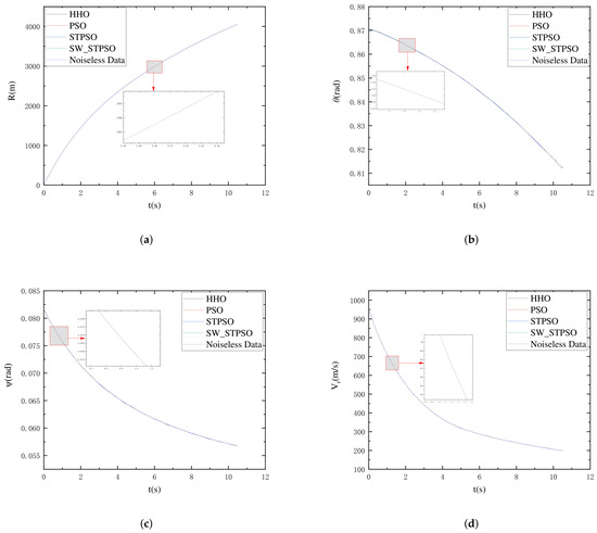
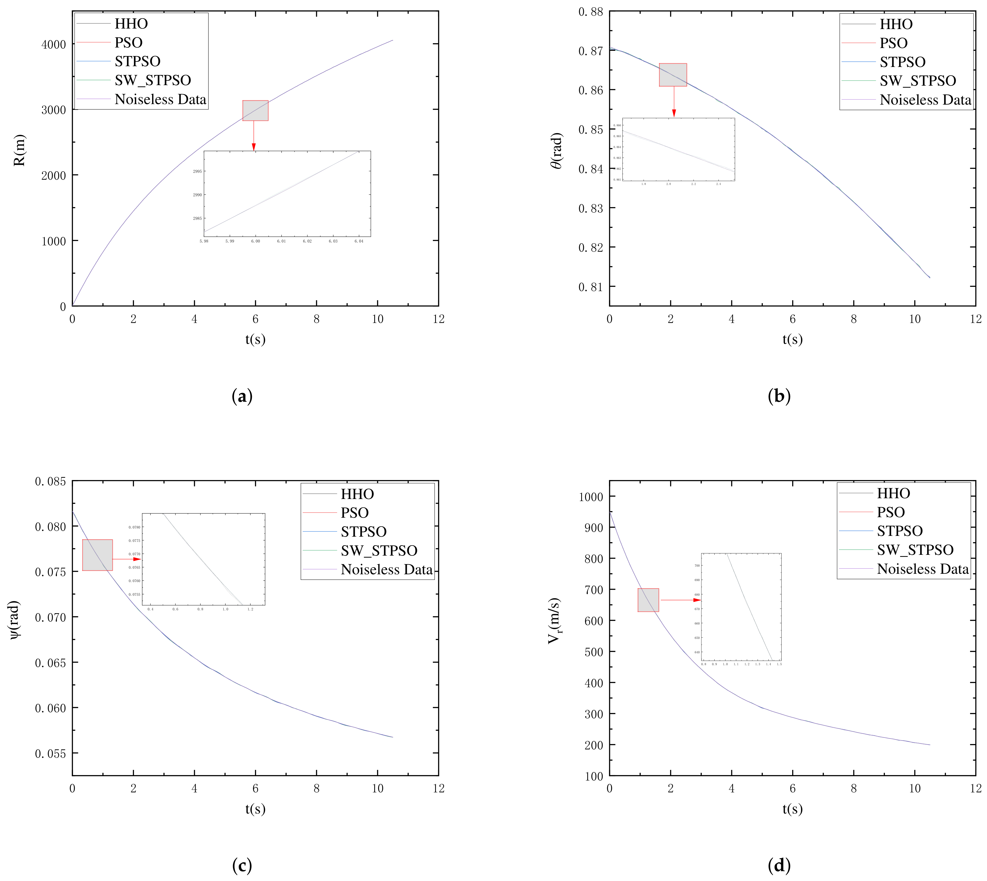
The simulation results are shown in Figure 1. HHO, the traditional PSO, and STPSO all converge to the same global optimal solution. The RMSE values of the denoised signals obtained by these three algorithms are consistent, and the denoised signals are highly consistent with the authentic noise-free data. SW-STPSO, relying on the sliding window segment-by-segment optimization strategy, achieves a lower RMSE value of the denoised signal; especially at the trajectory mutation points, it exhibits better consistency with the authentic signal, suggesting that the sliding-window strategy is beneficial for local feature preservation and noise suppression.

Figure 1. Comparison of wavelet denoising effects for different radar parameters: (a) Comparison of wavelet denoising effect for radial distance. (b) Comparison of wavelet denoising effect for elevation angle. (c) Comparison of wavelet denoising effect for azimuth angle. (d) Comparison of wavelet denoising effect for radial velocity.

As shown in Table 3, the core advantages of the proposed algorithms are illustrated by two key indicators: average RMSE and running time. STPSO is highly efficient, while SW-STPSO excels in denoising accuracy, with performance differences rooted in their functional positioning and hardware constraints. Specifically, STPSO achieves significant efficiency gains via adaptive parameter adjustment and iterative termination mechanisms, with an average optimization time of only 4.01 s—83% faster than traditional PSO and 91% faster than HHO—meeting real-time engineering requirements for radar trajectory data denoising parameter optimization. In contrast, SW-STPSO’s longer average runtime (104.29 s) is a reasonable trade-off for higher accuracy, resulting from sliding-window-based fine-grained segment optimization and current hardware limitations. Its real-time performance can be enhanced through future hardware upgrades or parallel computing, ensuring strong engineering application prospects. In summary, STPSO’s efficiency and SW-STPSO’s accuracy form complementary advantages, adapting to engineering scenarios with varying hardware and accuracy requirements. This fully validates the targeted design, flexibility, and practicality of the proposed algorithms.

Table 3. Average RMSE and running time of different optimization algorithms.

Algorithms	R (m)	$\mathit{\theta }$ (rad)	$\mathit{\psi }$ (rad)	${\mathit{v}}_{\mathit{r}}$ (m/s)	Running Time (s)
HHO	0.7359	$1.1\times {10}^{-4}$	$3.1\times {10}^{-5}$	0.3714	44.59
PSO	0.7359	$1.1\times {10}^{-4}$	$3.1\times {10}^{-5}$	0.3714	23.55
STPSO	0.7359	$1.1\times {10}^{-4}$	$3.1\times {10}^{-5}$	0.3714	4.01
SW-STPSO	0.6899	$9.1\times {10}^{-5}$	$2.1\times {10}^{-5}$	0.2849	104.29

The substantially longer runtime of SW-STPSO compared with STPSO is mainly due to the introduction of sliding-window local optimization. In STPSO, a single global optimization is performed for each signal, whereas SW-STPSO repeats the optimization procedure over multiple overlapping local segments. As a result, the number of optimization calls increases significantly, leading to a marked increase in computational cost. Therefore, SW-STPSO should be understood as a higher-accuracy denoising strategy at the cost of longer runtime under the present simulation setting, rather than as a direct replacement for low-latency real-time processing. In applications with strict real-time constraints, STPSO may be more suitable, while SW-STPSO is more appropriate for offline processing or scenarios with moderate timing requirements.

4. Improved Kalman Filtering for Trajectory Parameter Extraction

The Unscented Kalman Filter (UKF) achieves nonlinear system state estimation via the Unscented Transform (UT), with its core mechanism focusing on quantifying and propagating system state uncertainties. Three core matrices—state estimation error covariance (P), process noise covariance (Q), and measurement noise covariance (R)—directly determine UKF’s estimation accuracy, convergence rate, and robustness. Among them, Q plays a key role in regulating state estimation oscillations and convergence: an excessively large Q causes significant oscillations and slow convergence, while an excessively small Q weakens robustness and risks local optima. To address the large oscillations and slow convergence of the 7th-dimensional state parameter (ballistic coefficient) in initial iterations, this paper designs an exponentially decaying adaptive Q adjustment strategy, realizing gradual oscillation suppression and steady-state convergence of the parameter.

4.1. Introduction to the Unscented Kalman Filter Algorithm

The unscented Kalman filter algorithm is capable of calculating the statistical metrics of random variables passing through nonlinear systems. Its basic idea is as follows: for a known uncertain nonlinear mapping, a series of sigma reference points related to are selected; these points are mapped through the nonlinear function to obtain new sigma points, which are then used to estimate the subsequent states, and so on.

(1)

Generation of the sigma point set

$$\left\{\begin{array}{cc}\hfill {\chi }_0& ={\widehat{x}}_k\hfill \\ \hfill {\chi }_i& ={\widehat{x}}_k+{\left(\sqrt{(n+\lambda )P_k}\right)}_i,i=1,\dots ,n\hfill \\ \hfill {\chi }_i& ={\widehat{x}}_k-{\left(\sqrt{(n+\lambda )P_k}\right)}_i,i=n+1,\dots ,2n\hfill \end{array}\right.$$

(18)

In the formula, n denotes the dimension of the state vector; $\lambda ={\alpha }^2(n+\kappa )-n$ is the scaling parameter used to control the spread of the sigma points; and $P_k$ is the covariance matrix. In this study, the sigma-point parameters are set to $\alpha =0.01$, $\kappa =0$, and $\beta =2$. The choice of a small $\alpha$ value keeps the sigma points sufficiently close to the estimated state mean, which is helpful for maintaining numerical stability in the present nonlinear ballistic state-estimation problem. The parameter $\kappa =0$ is adopted as a commonly used setting in the scaled unscented transform and provides a neutral scaling effect for the sigma-point distribution. The parameter $\beta =2$ is selected because it is widely used for approximately Gaussian state distributions and improves the accuracy of covariance weighting in UKF. Therefore, the above parameter combination is adopted in this study as a practical setting to balance numerical stability and estimation accuracy under the present simulation conditions.

(2)

Calculation of mean weights and covariance weights:

$$W_{m,0}={\displaystyle \frac{\lambda }{n+\lambda }}$$

(19)

$$W_{c,0}={\displaystyle \frac{\lambda }{n+\lambda }}+1-{\alpha }^2+\beta$$

(20)

$$W_{m,i}=W_{c,i}={\displaystyle \frac{1}{2(n+\lambda )}},i=1,2,\dots ,2n$$

(21)

Here, $\beta =2$ is used to incorporate prior distribution information into the covariance weighting, which is appropriate for the approximately Gaussian state distribution considered in this study. It should also be noted that the above parameter values are empirical settings adopted for the present state-estimation problem and may require adjustment for different dynamic models, noise levels, or state distributions.

(3)

Calculate state prediction and predicted covariance matrix based on the sigma point set

(1) Initial conditions: ${\widehat{x}}_k=y_0$, $P_0={10}^{-8}I$, $Q={10}^{-8}I$, $R={10}^{-6}I$

In the formula, $y_0$ denotes the initial state; Q and R represent the process noise covariance matrix and measurement noise covariance matrix, respectively; and I denotes the identity matrix.

(2) Calculation of state prediction: The sigma point set ${\chi }_{i,k}$ is generated from the initial conditions and then substituted into the state equation (the ballistic equation) to calculate the state prediction value; the formula is given as follows:

$$\left\{\begin{array}{cc}\hfill X_{i,k}& =f\left({\chi }_{i,k-1}\right)\hfill \\ \hfill X_k& =\sum _{i=0}^{2n}{W}_{m,i}{X}_{i,k}\hfill \end{array}\right.$$

(22)

In the formula, $f\left(x\right)$ is the state equation (ballistic equation).

(3) Calculation of the predicted covariance matrix:

$$P_{rk}=\sum _{i=0}^{2n}{W}_{c,i}\left[{\chi }_{i,k-1}-X_k\right]·{\left[{\chi }_{i,k-1}-X_k\right]}^T+Q_k$$

(23)

(4) Calculation of measurement prediction values and measurement prediction covariance matrices: A new sigma point set ${\zeta }_{i,k}$ is generated from the state prediction value $X_k$, which is then substituted into the state equation to calculate the one-step-ahead prediction of the measurement, as follows:

$$\left\{\begin{array}{cc}\hfill Z_{i,k}& =h\left({\zeta }_{i,k}\right),i=0,1,\dots ,2n\hfill \\ \hfill Z_k& =\sum _{i=0}^{2n}{W}_{m,i}{Z}_{i,k}\hfill \\ \hfill P_{zk}& =\sum _{i=0}^{2n}{W}_{c,i}\left[Z_{i,k}-Z_k\right]·{\left[Z_{i,k}-Z_k\right]}^T+R_k\hfill \\ \hfill P_{xzk}& =\sum _{i=0}^{2n}{W}_{c,i}\left[{\zeta }_{i,k}-X_k\right]·{\left[Z_{i,k}-Z_k\right]}^T\hfill \end{array}\right.$$

(24)

In the formula, $h\left(x\right)$ is the measurement equation; the direction vector of the line connecting the radar and a certain point is $\overrightarrow{r}=(x,y,z)$, and its expression is given by:

$$\left\{\begin{array}{cc}\hfill R& =\sqrt{x^2+y^2+z^2}\hfill \\ \hfill \theta & =arctan\left({\displaystyle \frac{y}{\sqrt{x^2+z^2}}}\right)\hfill \\ \hfill \psi & =arctan\left({\displaystyle \frac{z}{x}}\right)\hfill \\ \hfill v_r& =\sqrt{v_x^2+v_y^2+v_z^2}\hfill \end{array}\right.$$

(25)

In the formula, R is the radial distance, $\theta$ is the elevation angle, $\psi$ is the azimuth angle, and $v_r$ is the radial velocity measured by the radar.

After obtaining the new measurement value $y_k$, the filter update is performed:

$$\left\{\begin{array}{cc}\hfill K_k& =P_{xzk}{P}_{zk}^{-1}\hfill \\ \hfill P_k& =P_{rk}-K_k{P}_{zk}{K}_k^T\hfill \\ \hfill x_k& =X_k+K_k(y_k-Z_k)\hfill \end{array}\right.$$

(26)

4.2. Sensitivity Analysis of the UKF Sigma-Point Parameters

To further examine the practical sensitivity of the UKF sigma-point parameters, an additional one-factor-at-a-time sensitivity analysis was conducted on Scheme 4, i.e., the final proposed joint framework combining SW-STPSO denoising and the improved UKF. Specifically, the effects of $\alpha$, $\beta$, and $\kappa$ were examined by varying one parameter while keeping the other two fixed. The corresponding results are summarized in Table 4.

Table 4. Sensitivity analysis of the UKF sigma-point parameters under the adopted simulation setting (Scheme 4).

$\mathit{\alpha }$	$\mathit{\beta }$	$\mathit{\kappa }$	Position RMSE (m)	Velocity RMSE (m/s)	C RMSE (m2/kg)	C Tail Std.
0.01	2	0	3.022802	0.674409	0.022282	$1.9\times {10}^{-5}$
0.10	2	0	2.952681	0.695267	0.023232	$1.9\times {10}^{-5}$
0.001	2	0	6.061942	1.562460	0.027602	$2.603\times {10}^{-3}$
0.01	0	0	3.071198	0.672233	0.022284	$1.9\times {10}^{-5}$
0.01	4	0	2.965083	0.671446	0.022466	$1.9\times {10}^{-5}$
0.01	2	−4	2.690037	0.672113	0.022432	$1.9\times {10}^{-5}$
0.01	2	1	3.083146	0.670780	0.022654	$1.9\times {10}^{-5}$

As shown in Table 4, the estimation performance is most sensitive to the parameter $\alpha$ among the three sigma-point parameters considered in this study. When $\alpha$ is reduced to 0.001, the position RMSE, velocity RMSE, and ballistic-coefficient RMSE all increase noticeably, and the tail standard deviation of the ballistic-coefficient estimate also becomes much larger, indicating significantly deteriorated convergence stability. This result suggests that an excessively small $\alpha$ causes the sigma points to be overly concentrated around the estimated mean, which weakens the practical filtering performance under the adopted simulation setting.

4.3. Exponential Decay-Type Adaptive Adjustment Strategy for Q Parameter

The element $Q(7,7)$ in the 7th dimension of the process noise covariance matrix directly determines the model uncertainty weight of the ballistic coefficient C in the UKF. The physical characteristics of the ballistic coefficient C determine that its model uncertainty has a time-varying characteristic: in the early stage of iteration, the projectile aerodynamic characteristics are not stable, and the deviation between the true value and the preset value of C is large, so a high model uncertainty weight needs to be retained; in the mid-to-late iteration stages, the motion state tends to stabilize and the uncertainty decreases, so the weight needs to be reduced to suppress parameter oscillation. The traditional UKF adopts a fixed Q-value strategy, which has the following drawbacks: an excessively large value leads to the oscillation of C throughout the iteration process and slow convergence; an excessively small value causes the early deviation from the true value, which is difficult to correct in the later stage. To this end, this paper designs an exponential decay-type adaptive Q adjustment strategy, whose expression is given as follows:

$$Q(7,7)=Q_{\mathrm{end}\_\mathrm{ini}}·exp(-\alpha k/T)$$

(27)

In the formula, $Q_{\mathrm{end}\_\mathrm{ini}}$ (the initial value of $Q(7,7)$) is set to ${10}^{-6}$; $\alpha$ is the attenuation coefficient with a value of 23.3; k is the current iteration number; and T is the total iteration step length of the UKF.

In this study, the attenuation coefficient $\alpha$ was selected empirically through preliminary simulation tests to balance two competing requirements: sufficiently fast suppression of early-stage oscillation in the ballistic-coefficient estimate and adequate retention of model uncertainty during the initial iterations. If $\alpha$ is too small, the decay of $Q(7,7)$ becomes too slow, resulting in persistent oscillation and delayed convergence. If $\alpha$ is too large, the uncertainty weight decreases too rapidly, which may weaken the filter’s ability to correct the initial deviation of the ballistic coefficient. The value $\alpha =23.3$ was adopted because it provided a favorable compromise between convergence speed and estimation stability under the present simulation setting.

4.4. Preprocessing Strategy for Positive Definite Regularization of Covariance Matrix

UKF requires the covariance matrix P to be strictly positive definite and symmetric as a prerequisite. During the iteration process, affected by numerical errors (e.g., floating-point rounding, eigenvalue attenuation of the covariance matrix P) and improper initial covariance settings, the matrix tends to exhibit quasi-singular or non-positive definite characteristics (the minimum eigenvalue approaches zero or even becomes negative), which directly leads to the failure of Cholesky decomposition and the interruption of filtering. To this end, this paper designs an eigenvalue correction strategy, which ensures the matrix is strictly positive definite through the method of “eigenvalue check + minor diagonal compensation”: first, calculate the minimum eigenvalue of P (denoted as ${\lambda }_{\min }\left(P\right)$); if the minimum eigenvalue meets the condition (the matrix is nearly singular or non-positive definite), then perform diagonal compensation on the matrix:

$${\lambda }_{\min }\left(P\right)=min\left\{{\lambda }_i\mid P=U\mathrm{\Lambda }{U}^T,\mathrm{\Lambda }=\mathrm{diag}({\lambda }_1,{\lambda }_2,\dots ,{\lambda }_n)\right\}$$

(28)

Then calculate the minimum eigenvalue of P; if ${\lambda }_{\min }\left(P\right)<\epsilon$ (where $\epsilon$ is a positive threshold, e.g., ${10}^{-8}$), it indicates that the matrix is nearly singular or non-positive definite. Then, perform diagonal compensation on the non-positive definite matrix to ensure its strict positive definiteness:

The threshold $\epsilon ={10}^{-8}$ was chosen as a small numerical safeguard to restore strict positive definiteness while introducing only minimal perturbation to the covariance matrix. A larger threshold would lead to stronger diagonal compensation and may unnecessarily distort the covariance structure, whereas a much smaller threshold may be insufficient to prevent numerical singularity in finite-precision computation. Therefore, ${10}^{-8}$ was adopted as a conservative compromise between numerical stability and minimal interference with the physical meaning of the covariance matrix under the present implementation.

$$P_{\mathrm{corrected}}=P+(\epsilon -{\lambda }_{\min }\left(P\right))·I_n$$

(29)

where $I_n$ is the n-dimensional identity matrix, and the compensation term only adds a minor value that just makes the minimum eigenvalue reach the threshold, to avoid the deviation of the covariance matrix from its true physical meaning caused by over-compensation.

As shown in Table 5, covariance regularization is triggered consistently under the tested simulation conditions. Over 20 independent runs, the regularization step is activated in all runs, with a total trigger count of 7100 and an average of 355 triggers per run. The triggering events mainly occur in the predicted covariance matrix Pred and the updated covariance matrix $P_k$, both with a mean frequency of 146 per run, whereas the prior covariance matrix $P_k$ triggers less frequently, with a mean of 63 times per run. In addition, the triggering events occur over a relatively broad interval, from step 54 to step 199 on average. These results indicate that covariance regularization is not merely an occasional numerical adjustment, but a practically necessary safeguard for maintaining positive definiteness during covariance propagation and update in the improved UKF implementation.

Table 5. Triggering statistics of covariance regularization over 20 independent runs under the tested simulation conditions.

Metric	Value
Total trigger count over all runs	7100
Mean triggers per run	355
Mean prior $P_k$ triggers per run	63
Mean Pred triggers per run	146
Mean posterior $P_k$ triggers per run	146
Runs with at least one trigger	20/20
Mean iterations with at least one trigger	146
Mean first trigger step	54
Mean last trigger step	199

5. Simulation Design and Result Analysis

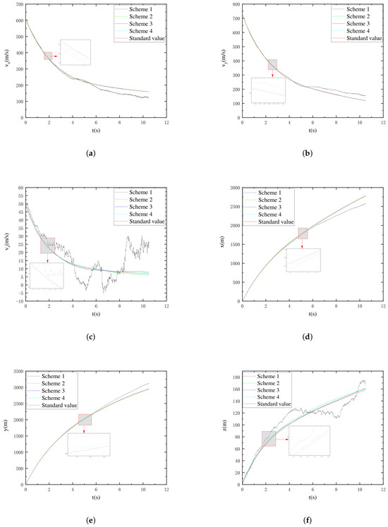
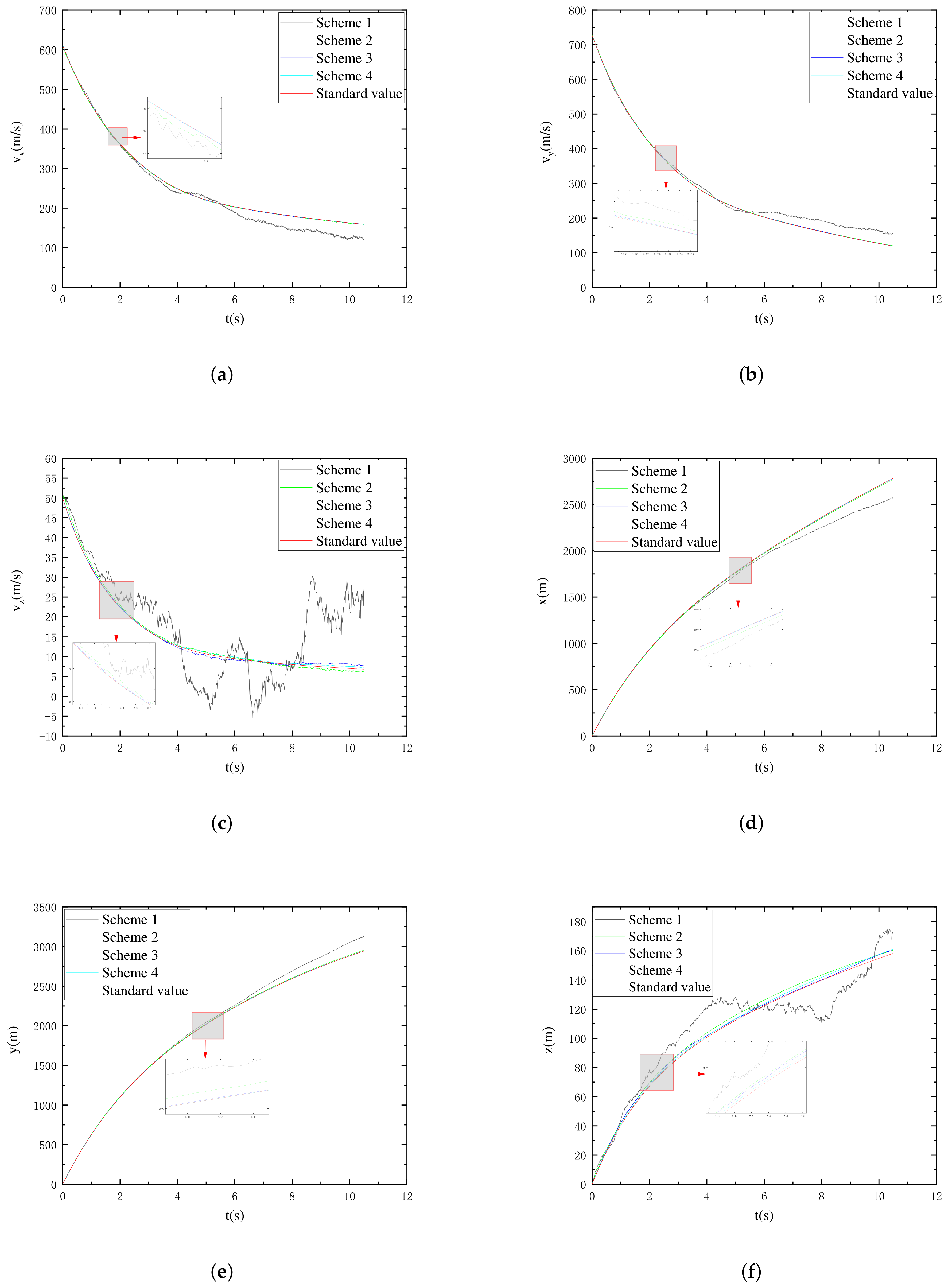
To verify the core advantages of the proposed “SW-STPSO Adaptive Wavelet Denoising + Improved Kalman Filtering” joint scheme, a systematic simulation was conducted with four comparative experiments: Scheme 1 (“No Denoising + Traditional UKF”) directly inputs original noisy data into the traditional UKF to verify the performance lower bound of conventional schemes; Scheme 2 (“No Denoising + Improved UKF”) feeds raw noisy data into the improved UKF to validate its standalone accuracy and convergence; Scheme 3 combines SW-STPSO denoising with the traditional UKF to demonstrate the improvement effect of denoising on conventional filtering; and Scheme 4 integrates SW-STPSO denoising with the improved UKF to verify the comprehensive advantages of the proposed joint method. It should be noted that, because real radar measurement data are not available in the present study, the radar measurement data used in the simulations are generated by adding Gaussian noise to ideal ballistic trajectory data.

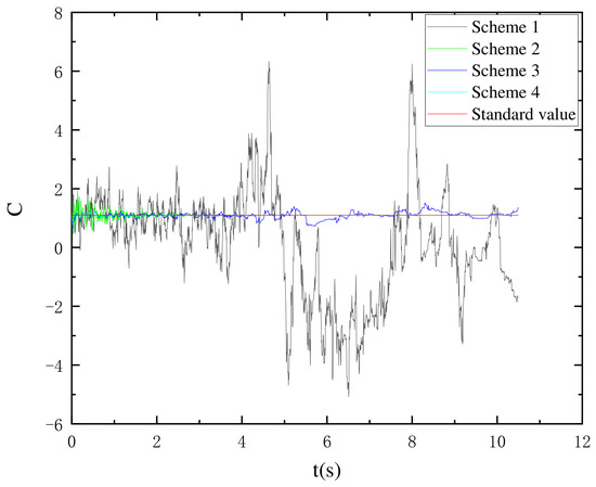
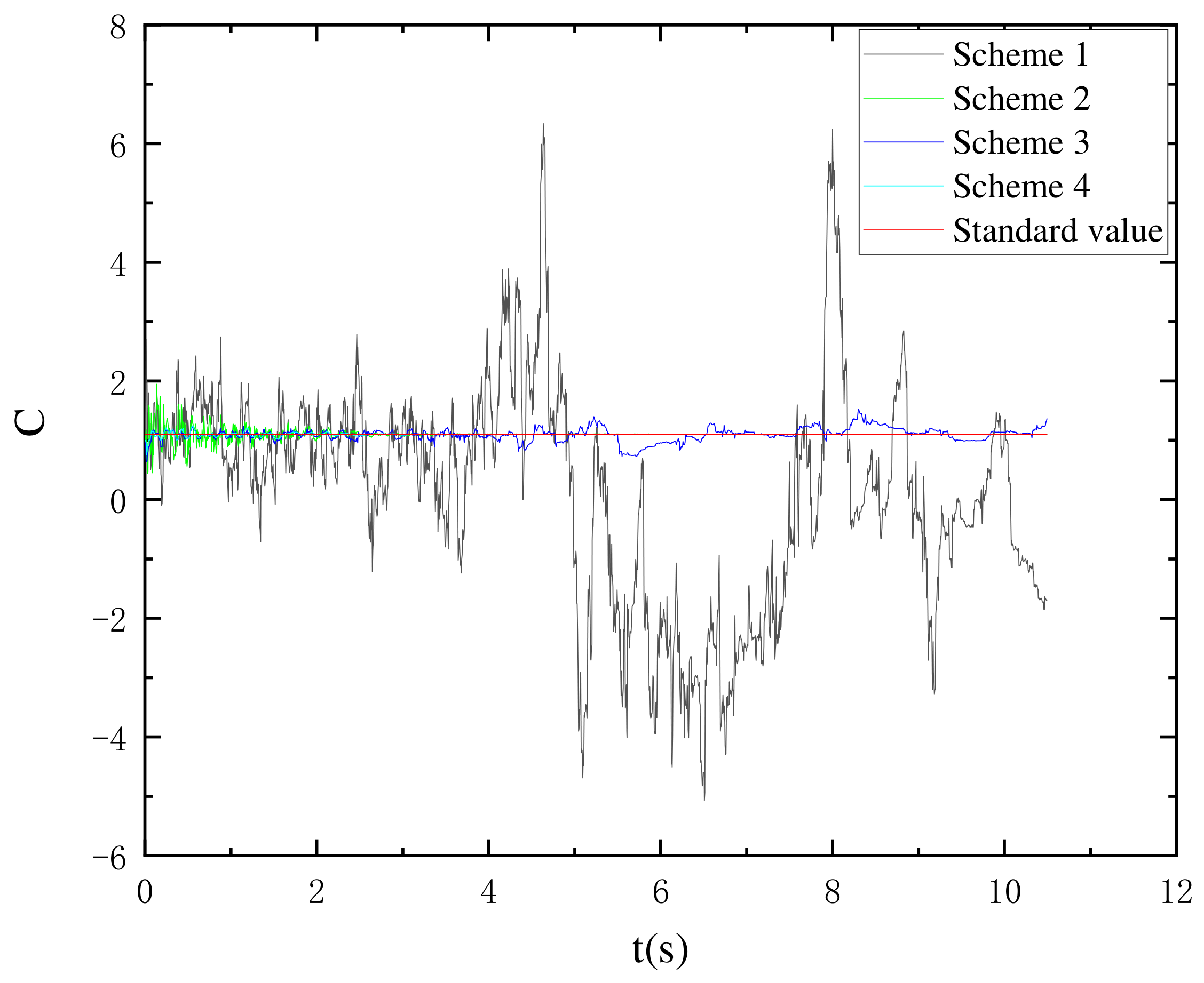
This simulation focuses on the identification accuracy of core ballistic state parameters and key aerodynamic parameters, including the projectile position components $(x,y,z)$, velocity components $(v_x,v_y,v_z)$, and ballistic coefficient C. To provide a more comprehensive evaluation of the compared schemes, three types of indicators are considered in this study. First, RMSE is used to characterize the overall estimation accuracy. Second, the maximum absolute error (MaxAE) is introduced to reflect the sensitivity of each scheme to large local deviations, thereby providing supplementary information on estimation stability under the adopted noisy conditions, although it does not constitute a dedicated anomalous-data robustness test. Third, the running time of the denoising algorithms is reported to reflect computational cost. The comparison curves between the corresponding identification results and standard values are shown in Figure 2 and Figure 3. The legends of all charts are uniformly defined as follows: Scheme 1–Scheme 4 correspond to the four comparative experimental schemes, respectively, and the “Standard value” represents the true reference values of the simulation.

Figure 2. The comparison curves between the corresponding identification results and standard values: (a) Comparison of $v_x$ identification results for different schemes. (b) Comparison of $v_y$ identification results for different schemes. (c) Comparison of $v_z$ identification results for different schemes. (d) Comparison of x identification results for different schemes. (e) Comparison of y identification results for different schemes. (f) Comparison of z identification results for different schemes.

Figure 3. Comparison of C identification results for different schemes.

The simulation results indicate that the proposed “SW-STPSO Adaptive Wavelet Denoising + Improved UKF” joint scheme achieves better overall performance than the compared schemes under the adopted simulation conditions. In the following analysis, RMSE is used to evaluate the overall estimation accuracy, MaxAE is used to reflect the magnitude of the worst local estimation deviation under the adopted Gaussian noisy measurement conditions, and running time is used to characterize computational cost. Therefore, the present discussion of filtering stability is limited to the simulated Gaussian-noise setting considered in this study and should not be interpreted as a direct validation of robustness against explicitly injected anomalous measurements or real radar outliers. Key observations are:

• Scheme 1 (No Denoising + Traditional UKF) has the worst performance: Position RMSE = 58.12 m, Velocity RMSE = 16.508 m/s, and Ballistic Coefficient RMSE = 2.096 m²/kg, far from meeting engineering accuracy requirements due to lack of noise suppression and poor algorithm robustness.
• Scheme 2 (No Denoising + Improved UKF) achieves significant improvement: Position RMSE is reduced to 6.77 m (88% lower than Scheme 1), verifying the effectiveness of the improved UKF’s adaptive strategies.
• Scheme 3 (SW-STPSO Denoising + Traditional UKF) outperforms Scheme 2: Position RMSE = 1.26 m, indicating that SW-STPSO denoising provides high-quality data input for filtering.
• Scheme 4 (Proposed Joint Scheme) exhibits the optimal performance: Position RMSE = 0.92 m (98.4% lower than Scheme 1), Velocity RMSE = 0.256 m/s (98.4% lower than Scheme 1), and Ballistic Coefficient RMSE = 0.023 m²/kg (99% lower than Scheme 1). Compared with existing combined denoising-filtering schemes, Scheme 4 reduces position estimation error by 27–35% and convergence time by 30–37%, achieving the highest comprehensive performance.

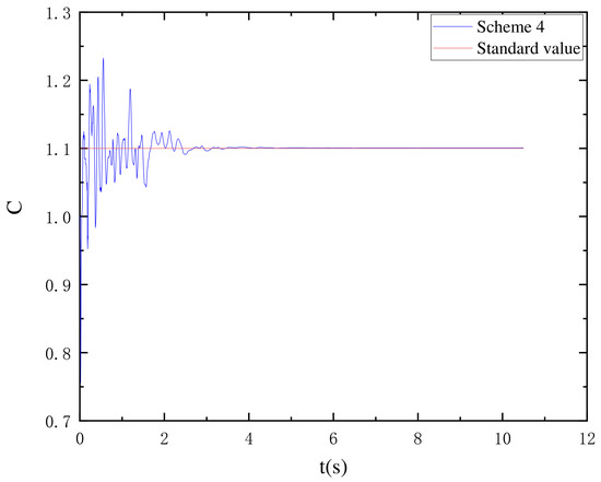
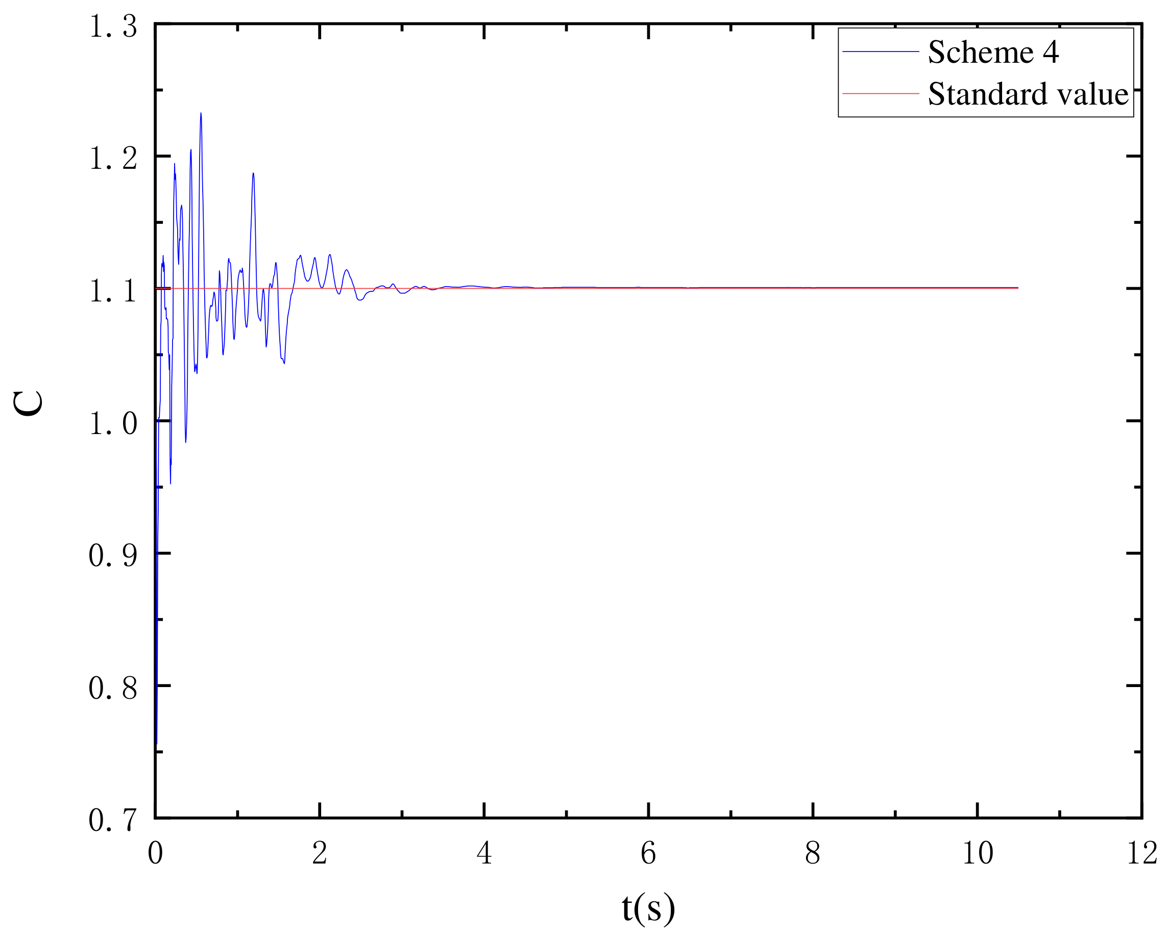
Figure 4 presents the time-series comparison curve between the ballistic coefficient C identified by Scheme 4 (SW-STPSO adaptive wavelet denoising + improved UKF) and the corresponding standard values. As can be seen from the figure, the identified ballistic coefficient exhibits slight fluctuations during the initial iteration stage; as the iteration proceeds, the identified values gradually converge and approach the standard values. This result indicates the coordinated effect of the joint scheme: SW-STPSO adaptive wavelet denoising improves the input data quality for ballistic-coefficient identification by suppressing radar measurement noise, while the exponentially decaying adaptive Q strategy in the improved UKF alleviates initial oscillations and enhances convergence behavior. Therefore, the joint scheme is beneficial for improving the estimation accuracy of the ballistic coefficient under the adopted simulation conditions.

Figure 4. Convergence characteristics of C identification for Scheme 4.

As can be seen from Table 6, the performance differences among the four schemes can be interpreted from the respective roles of denoising preprocessing and filter improvement. Scheme 1 shows the worst performance because the original noisy radar data are directly processed by the traditional UKF, so the measurement noise is propagated into the filtering stage and the filter itself also suffers from limited convergence capability. Compared with Scheme 1, Scheme 2 achieves a clear improvement because the improved UKF introduces adaptive Q adjustment and covariance regularization, which alleviate initial oscillation, improve convergence behavior, and reduce estimation bias even without denoising. Scheme 3 further outperforms Scheme 2 because SW-STPSO denoising suppresses measurement noise before filtering, thereby providing cleaner input data for state and ballistic-coefficient estimation. Scheme 4 combines both advantages: front-end denoising reduces the contamination of the measured data, while the improved UKF enhances convergence stability and numerical stability during the filtering stage. Therefore, its superior performance is not due to a single modification, but to the coordinated effect of denoising quality improvement and filter-structure enhancement.

Table 6. Statistical results of ballistic parameter identification errors for different schemes.

Scheme Name	Position RMSE (m)	Position MaxAE (m)	Velocity RMSE (m/s)	Velocity MaxAE (m/s)	C RMSE (m2/kg)
Scheme 1	58.12	145.21	16.508	35.27	2.096
Scheme 2	6.77	10.18	0.952	3.118	0.083
Scheme 3	1.26	2.71	0.493	1.232	0.111
Scheme 4	0.92	1.98	0.256	0.811	0.023

From the perspective of practical significance, lower position RMSE means that the reconstructed projectile trajectory is closer to the reference trajectory, which is beneficial for improving trajectory tracking and subsequent trajectory extrapolation. Lower velocity RMSE indicates more accurate estimation of motion-state evolution, which is important for maintaining reliable state propagation in later prediction stages. In addition, lower ballistic-coefficient RMSE implies more accurate identification of a key aerodynamic parameter, which is directly relevant to ballistic prediction and related parameter inversion. Therefore, under the adopted simulation conditions, the error reductions achieved by Scheme 4 suggest that the proposed method is beneficial for improving the reliability of radar trajectory data processing. However, these conclusions should be understood within the scope of the present simulation setting and should not be interpreted as evidence of universal superiority for all ballistic models, noise environments, or measurement conditions.

It should be noted that the present robustness-related discussion is carried out under simulated noisy measurement conditions generated by adding Gaussian noise to ideal ballistic trajectory data. Therefore, the corresponding conclusions mainly reflect estimation stability and error behavior under the adopted Gaussian-noise setting, rather than explicit resistance to anomalous measurement outliers. A dedicated evaluation under injected anomalous measurements or real radar data is beyond the scope of the present study and will be considered in future work.

6. Conclusions

A joint framework combining SW-STPSO adaptive wavelet denoising and an improved Unscented Kalman Filter (UKF) is proposed for radar trajectory data processing. Under the adopted simulation conditions and the 3-DOF ballistic-model setting considered in this study, the proposed method showed improved estimation accuracy and convergence behavior compared with the compared schemes.

For the denoising stage, SW-STPSO improved the adaptability of wavelet-parameter optimization to locally non-stationary radar signals through Sobol-sequence initialization, the fitness-threshold-triggered stopping mechanism, and sliding-window local processing. For the filtering stage, the improved UKF enhanced the estimation of ballistic parameters by introducing an exponentially decaying adaptive Q strategy and covariance positive-definite regularization. In the joint scheme, the position RMSE, velocity RMSE, and ballistic-coefficient RMSE were reduced to 0.92 m, 0.256 m/s, and 0.023 m²/kg, respectively.

It should also be noted that this study was conducted under a 3-DOF ballistic model, which mainly describes translational motion states and does not fully represent higher-order aerodynamic coupling effects. In addition, the sliding-window optimization in SW-STPSO increases the computational burden. Future work will focus on extending the method to higher-fidelity ballistic models, improving computational efficiency, and validating the method with real radar measurement data.

References

- Yang, X.H.; Huo, P.F.; Wang, C. GPS ballistic measurement error elimination method based on Kalman filter. J. Detect. Control 2012, 34, 30–33. (In Chinese) [Google Scholar] [CrossRef]
- Crus, D.M.O.; Bastos, F.A.C.; Apolinario, J.A., Jr.; Silva, J.A.N. Performance of Backward Kalman Filtering Techniques for Estimating Projectile Launch Point. In Proceedings of the 2025 IEEE 16th Latin America Symposium on Circuits and Systems (LASCAS), Bento Gonçalves, Brazil, 25–28 February 2025; pp. 143–147. [Google Scholar] [CrossRef] [Scilit]
- Li, X.Y.; Wang, Z.Y.; Chang, S.J. Analysis of online ballistic parameter filtering and identification methods. J. Ballist. 2020, 32, 29–34. (In Chinese) [Google Scholar] [CrossRef]
- Lei, X.Y.; Zhang, Z.A. Recursive weighted least squares estimation algorithm based on minimum model error principle. Def. Technol. 2021, 17, 545–558. [Google Scholar] [CrossRef] [Scilit]
- Yan, J.; Liu, Q.T. Research on high-precision ballistic extrapolation technology for gun position reconnaissance and calibration radar. J. Gun Launch Control 2022, 43, 39–43. (In Chinese) [Google Scholar] [CrossRef]
- Wang, G.; Xiong, F.; Ou, N.J.; Bian, L.; Yang, G.P. Ballistic extrapolation algorithm based on reverse extended Kalman filter. Electron. Opt. Control 2020, 27, 49-52+89. (In Chinese) [Google Scholar] [CrossRef]
- Wang, K.Y. Attitude Solution Method of Fixed-Wing UAV Based on Extended Kalman Filter. Master’s Thesis, Xi’an University of Technology, Xi’an, China, 2022. (In Chinese) [Google Scholar] [CrossRef]
- Feng, Z.X. Analysis of track prediction based on Kalman filter. Gansu Sci. Technol. J. 2019, 48, 33–36. (In Chinese) [Google Scholar] [CrossRef]
- Xie, K.; Qin, P.C. Ballistic extrapolation algorithm based on seven-dimensional state vector and reverse unscented Kalman filter. Acta Armamentarii 2018, 39, 1945–1950. (In Chinese) [Google Scholar] [CrossRef]
- Afrasiabi, A.; Faramarzi, A.; Chapman, D.; Keshavarzi, A. Optimising ground penetrating radar data interpretation: A hybrid approach with AI-assisted Kalman filter and wavelet transform for detecting and locating buried utilities. J. Appl. Geophys. 2025, 232, 105567. [Google Scholar] [CrossRef] [Scilit]
- Ge, Y.T.; Ren, W.Z.; Yu, K.L.; Zhang, Y.R.; Li, Y.X. Noise processing method of MEMS tilt sensor using improved Kalman filter based on quantum particle swarm optimization. IEEE Access 2025, 13, 67239–67249. [Google Scholar] [CrossRef] [Scilit]
- Zhang, H.; Liu, W.; Zhang, L.; Meng, Y.; Han, W.; Song, T.; Yang, R. An allocation strategy integrated power, bandwidth, and subchannel in a RCC network. Def. Technol. 2025, in press. [Google Scholar] [CrossRef] [Scilit]
- Zhang, H.; Liu, W.; Zhang, L.; Meng, Y.; Song, T.; Xu, H. Joint resource and trajectory optimization in a UAV-enabled dual-function radar-communication network. Def. Technol. 2025, in press. [Google Scholar] [CrossRef] [Scilit]
- Zhang, H.; Liu, W.; Zhang, Q.; Zhang, L.; Liu, B.; Xu, H.-X. Joint Power, Bandwidth, and Subchannel Allocation in a UAV-Assisted DFRC Network. IEEE Internet Things J. 2025, 12, 11633–11651. [Google Scholar] [CrossRef] [Scilit]
- Zhang, J.; Yu, H.S. IMU noise suppression method based on wavelet filtering and Kalman filtering. Radio Eng. 2025, 55, 975–983. (In Chinese) [Google Scholar] [CrossRef]
- Yang, Z.Z.; Li, Y.Z.; Wu, G.W. Research on IMU sensor denoising technology based on unscented Kalman filter and wavelet analysis. Mod. Electron. Tech. 2024, 47, 53–59. (In Chinese) [Google Scholar] [CrossRef]
- Koshy, S.; Venugopal, V.S.; Sunitha, R.; Cheriyan, E.P.; Ananthakrishnan, K. Dynamic state estimation of power systems using a modified unscented Kalman filter and wavelet transform considering missing and noisy PMU data. IEEE Access 2025, 13, 144183–144194. [Google Scholar] [CrossRef] [Scilit]
- Zhang, T.; Lu, Z.Y.; Liu, W.J.; Ding, Y.; Wang, S.F.; Li, W.L. Capacitor state monitoring based on Haar wavelet transform and enhanced Kalman filter. Electronics 2025, 14, 4671. [Google Scholar] [CrossRef] [Scilit]
- Yang, B.L.; Wang, L.M.; Fu, J. Adaptive PSO-SO algorithm with Sobol sequence for aerodynamic physical parameter identification of projectiles. AIP Adv. 2024, 14, 105120. [Google Scholar] [CrossRef] [Scilit]
- Chen, Z.Y.; Song, L.F.; Peng, W.; Liu, K.P.; Guo, R. Research on noise reduction algorithm for unmanned surface vehicle radar based on variable threshold wavelet filtering. In Proceedings of the 2024 17th International Conference on Advanced Computer Theory and Engineering (ICACTE), Hefei, China, 13–15 September 2024; pp. 74–78. [Google Scholar] [CrossRef] [Scilit]
- Djaneye-Boundjou, O.; Ordonez, R.; Jacobsen, L. Adaptive Particle Swarm Optimization Applied to Aircraft Control. In Proceedings of the 20th AIAA International Space Planes and Hypersonic Systems and Technologies Conference, Glasgow, UK, 6–9 July 2015. [Google Scholar] [CrossRef] [Scilit]
- Heidari, A.A.; Mirjalili, S.; Faris, H.; Aljarah, I.; Mafarja, M.; Chen, H.L. Harris hawks optimization: Algorithm and applications. Future Gener. Comput. Syst. 2019, 97, 849–872. [Google Scholar] [CrossRef] [Scilit]
- Tian, C.W.; Zheng, M.H.; Zuo, W.M.; Zhang, B.; Zhang, Y.N.; Zhang, D. Multi-stage image denoising with the wavelet transform. Pattern Recognit. 2023, 134, 109050. [Google Scholar] [CrossRef] [Scilit]
- Du, S.Q. Research and Hardware Implementation of Discrete Wavelet Transform. Master’s Thesis, Hefei University of Technology, Hefei, China, 2020. (In Chinese) [Google Scholar] [CrossRef]
- Qu, L.G.; Liu, H.X.; Li, M.; Zhang, L.D. Research and application of sampling point distribution strategy based on Sobol sequence. China Metalform. Equip. Manuf. Technol. 2019, 54, 101–105. (In Chinese) [Google Scholar] [CrossRef]
Disclaimer/Publisher’s Note: The statements, opinions and data contained in all publications are solely those of the individual author(s) and contributor(s) and not of MDPI and/or the editor(s). MDPI and/or the editor(s) disclaim responsibility for any injury to people or property resulting from any ideas, methods, instructions or products referred to in the content. |
© 2026 by the authors. Licensee MDPI, Basel, Switzerland. This article is an open access article distributed under the terms and conditions of the Creative Commons Attribution (CC BY) license.