Article

Response Surface-Based Predictive Modeling of Cavitation Damage in Morning-Glory Spillways Under Uncertainty

by
Masoud Ghaffari
1,
Mehdi Azhdary Moghaddam
1,*,
Gholamreza Aziziyan
1 and
Mohsen Rashki
2
1
Civil Engineering Department, University of Sistan and Baluchestan, Zahedan 98167-45845, Iran
2
Architectural Engineering Department, University of Sistan and Baluchestan, Zahedan 98167-45845, Iran
*
Author to whom correspondence should be addressed.
Modelling 2026, 7(3), 78; https://doi.org/10.3390/modelling7030078
Submission received: 1 November 2025 / Revised: 29 December 2025 / Accepted: 2 January 2026 / Published: 23 April 2026

Abstract

Cavitation damage poses a serious threat to the reliability of morning-glory spillways. This study aims to develop a reliability framework for predicting cavitation damage probability under uncertain operational conditions for the Haraz Dam spillway. Cavitation analysis in such structures exhibits inherent nonlinearity and uncertainty, complicating accurate damage prediction. This study incorporates model uncertainties to assess cavitation responses at multiple points on the Haraz Dam morning-glory spillway. Three-dimensional flow simulations were performed using Computational Fluid Dynamics (CFD) and validated against an experimental model from the Iran Water Research Institute, showing satisfactory agreement. Statistical parameters and probability density functions (PDFs) for key uncertainties were determined using the Shapiro–Wilk test. A total of 35 simulation runs, designed via the Central Composite Design (CCD) method, were conducted using Latin Hypercube Sampling (LHS). These simulations incorporated inter-uncertainty correlations and predicted cavitation damage responses at ten critical spillway locations through Response Surface Methodology (RSM). Both linear and second-order response functions were formulated based on interactions among model uncertainties. The results indicated a strong correlation (R2 > 0.95) between numerical model outputs and RSM predictions, with the maximum RSM errors remaining within acceptable thresholds. Among the uncertainty factors, the inflow velocity demonstrated the highest contribution (>50%) to cavitation damage responses. These outcomes advance the understanding of cavitation mechanisms and provide a reliable methodology for evaluating damage risks in morning-glory spillways under uncertain operational conditions.

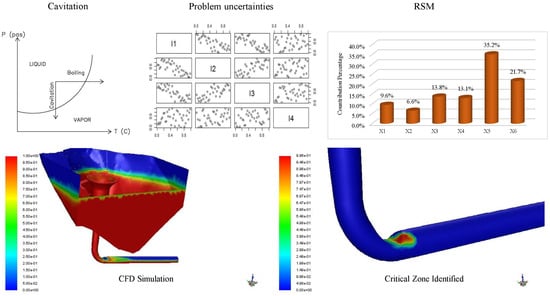
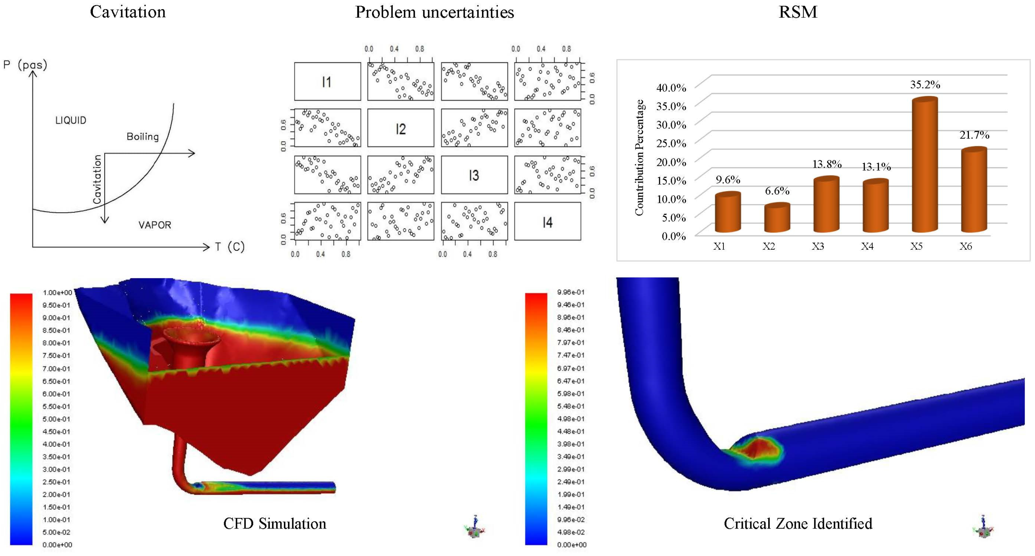
Graphical Abstract

1. Introduction

Research on flood control systems, such as spillways, is critically important as floods are natural disasters that frequently result in significant financial losses and casualties. Uncertainties in parameters such as hydraulic flow, applied loads, environmental conditions, material properties, and constructional defects can unexpectedly impact spillways and their structural performance. Therefore, these factors must be thoroughly considered during the design process. Spillways are highly complex, and managing cavitation is particularly challenging due to the numerous factors that must be accounted for [1]. Aydin et al. [2] investigated the impact of cone dimensions on the hydraulic performance of shaft siphon spillways. Using CFD numerical simulations, they demonstrated that increasing the shaft opening significantly reduces vacuum velocity in the siphon, thereby mitigating cavitation along the shaft surface. In the cavitation mechanism, a decrease in pressure at constant temperature causes the liquid to form an air–vapor mixture due to static and dynamic factors. The resulting bubbles grow gradually and collapse under high-pressure conditions. When the collapse occurs near a concrete surface, it is asymmetric and leads to jet formation, which can cause structural damage [3]. Mathematically, cavitation is best forecasted using the cavitation index (σ), defined by Equation (1) [4]:
σ = P 0 P V 0.5 ρ V 2                
where P0 is the local pressure at the intended point, Pv is the water vapor pressure, V is the local velocity, and ρ is the fluid density. In a study on spillway damage, Manogaran et al. [5] developed numerical and experimental models to mitigate failure by calculating the minimum velocity required to control erosion and cavitation. Wuyi et al. [6] evaluated cavitation damage on rapid-flow chute spillways using computational fluid dynamics (CFD) models, numerical predictions, and risk analyses, identifying high-cavitation-potential areas on the concrete spillway surface. Sharifi [7] investigated stepped spillway performance by proposing upward/downward-shaped step surfaces as an alternative to traditional horizontal designs. Using 2D CFD modeling, the study highlighted how modified step geometries influence skimming flow dynamics, vortex formation, and structural resilience. Kalateh and Aminvash [8] optimized aerator positioning in morning-glory spillways using CFD, demonstrating 50% pressure reduction in vertical shafts and 81.6% lower cavitation risk in elbows through two-phase flow management. Recent breakthroughs have dramatically improved our ability to predict cavitation risks.
Recent advancements by Reza and Dziedzic [9] have significantly progressed this field through their enhanced Bayesian risk assessment model. Their meta-analysis of over 100 studies not only critically evaluated Bayesian methodologies but also established improved guidelines for dam safety protocols and emergency preparedness measures. Using FLOW-3D v11.1, Enjilzadeh and Nohani [10] investigated hydraulic flow parameters for different discharges at the Alborz Dam morning-glory spillway. They compared their results with experimental data, reporting errors of 6.4% for passing discharge and 7.6% for flow depth over the spillway crest. The Volume of Fluid (VOF) model is a well-established method for simulating complex air–water interfaces in hydraulic structures, as successfully demonstrated in high-accuracy studies of dike-induced flows using OpenFOAM v2512 [11]. Bordbar et al. [12] developed hydraulic models for both smooth and stepped morning-glory spillways, demonstrating that a 7-step spillway design was most effective in preventing concrete erosion, with a regression index of 99%.
Foroudia and Barati [1] examined spillway cavitation, identifying the cavitation index as the most critical factor for various spillway angles. Modern analysis employs advanced methods like finite-element strength-reduction for safety factor estimation and Bayesian global optimization for boundary determination [13]. These uncertainties significantly influence failure probabilities (Pf), as established by Yen et al. [14] and further developed by Yen and Tung [15], who demonstrated the impact of model and parameter uncertainties. Motahari Moghadam et al. [16] numerically investigated hydraulic erosion in spillways, focusing on flow parameters under single- and double-gate configurations. Using CFD modeling of the Romaine IV spillway, they demonstrated that double-gate setups promote uniform flow distribution, while single-gate designs cause higher depth fluctuations. Zhou et al. [17] further elucidated how inflow velocity and angle govern cavitation dynamics, including bubble formation and collapse mechanisms. Mozaffari et al. [18] used CFD models to control spillway discharge, achieving a good comparison between numerical and experimental models. They reported acceptable errors based on the calculated mean absolute error (MAER) and regression coefficient (R). Kocaer et al. [19] conducted turbulent flow studies on chute spillways using the ANSYS Fluent v19.0 model, finding a strong correlation between numerical and experimental parameters.

1.1. Response Surface Method (RSM)

RSM is a set of mathematical and statistical techniques used to adapt empirical data to polynomial models. It allows for the simultaneous and sequential study of variable effects and parameter interactions to identify optimal solutions. The model used in RSM is typically a complete quadratic equation (or its reduced form), expressed as follows (Equation (2)) [20]:
y = β 0 + i = 1 k β i x i + i = 1 k β i i x i 2 + β i j x i x j + ε
where β0, βi, βii, and βij are, respectively, constant, linear, quadratic term, and factor interaction coefficients, and X i and X j are coded independent variables. The matrix notation is as follows (Equation (3)):
y = X β + ε
where y is an n × 1 response vector, X is an n × p independent variable vector, Β is a p × 1 regression coefficient vector, and ε is an n × 1 random error vector. The difference between responses y i and predicted values y ^ i is displayed with e i (residual value). The least square method (LSM) is used to determine β parameters. The sum of squares error (SSE) is defined as follows (Equation (4)) [21]:
S S E = i = 1 n ( y i y ^ i ) 2 = i = 1 n ( e i ) 2 = e T e
where n is the number of observations and T is the number of regression coefficients. Identifying different uncertainty sources is necessary to accurately predict and describe the performance of the structures’ destructive factors [22]. Uncertainties in hydraulic engineering systems can be hydrologic, hydraulic, structural, and economic [23]. Since spillway cavitation performance is influenced by uncertainties such as fluid properties, hydraulic flow, spillway geometry, material strength, construction quality, and human error, simulation methods require numerous samples to account for the probability distribution of these uncertainties.
RSM has been proposed alongside simulation methods to address this issue with reduced computational effort [24,25]. Using RSM, Keshtegar et al. [26] developed a model that predicted river flow with an acceptable error rate using polynomial functions of the second to fifth degree. Considering uncertainty sources and using RSM, Bayari et al. [27] conducted a probabilistic assessment of structures, fitting the boundary condition function to a second-degree polynomial and calculating the expected damage probability based on it.
Accounting for temperature uncertainty, Yang et al. [28] used RSM to study the safety factor in arch dams by analyzing failure probability in their body and foundation. Their model, analyzed in ANSYS, evaluated strength and stability reliability, demonstrating accurate results. Hammed et al. [29] used high-order (second to fifth) RSM to investigate resistant concrete and predict its strength while considering expected uncertainties. Zhang et al. [30], incorporating time-dependent factors and reliability analysis with RSM, rapidly predicted the stability of steep rock-fill dams and identified their safe zones.

1.2. Research Methodology

This study aims to use RSM and numerical techniques to investigate cavitation damage on the morning-glory spillway of Haraz Dam. Since the damage is complex, the boundary condition function lacks a clear form and requires extensive calculations for its estimation, making it a less explored area in research. While Yang et al. [28] assessed only one uncertainty parameter to estimate responses, this study examines six parameters to develop response surface functions. Unlike Zhang et al. [30] and Bayari et al. [27], who applied correlation matrices derived from similar studies, this research used the Shapiro–Wilk test to identify and extract statistical parameters, including the correlation matrix, specifically for the Haraz Dam spillway.
To derive numerical results, 35 simulations were conducted using the Latin Hypercube Sampling (LHS) method, analyzed with the ANSYS Fluent 3D model. Cavitation responses were predicted at 10 critical points on the spillway using the Central Composite Design (CCD) for RSM. Finally, the association rate and interactions of each uncertainty parameter were evaluated to predict cavitation responses at specific points on the spillway.
This research comprehensively identifies uncertainties affecting cavitation behavior and quantifies performance objectives for spillways by assessing response levels. Another significant contribution of this study is that its equations and response functions can be used in future research to greatly reduce computational costs.


2. Materials and Methods

This study investigates cavitation damage on the morning-glory spillway of the Haraz Dam in Iran. The key specifications of the dam and its spillway are summarized in Table 1.
To analyze the flow, the ANSYS Fluent 19.0 software uses Reynolds-Average Navier–Stokes equations (RANS), which are discretized by the finite volume method, and to solve the Fluent problems, analyses of the conservation equations (continuity, momentum, and energy) are an important step because in each iteration, they should be repeatedly solved to solve the problem and reach convergence. The present computational model constitutes a full three-dimensional representation of the fluid domain. The governing equations are solved within the entire discretized volume. Equation (5) (RANS), which expresses the rules governing the flow of an incompressible viscous fluid, mathematically expresses the mass and momentum stability as follows [32]:
ρ U i t + ρ U i U i x j = p x i + x j ( 2 μ S i j ρ u j u i ¯ )
where u j u i ¯ , Ui, xi, t, and P are the Reynolds stress tensor, velocity, coordinate, time, and pressure, respectively, and ρ, µ, and Sij are density, dynamic viscosity, and strain rate tensor, respectively. Among models used to accurately simulate turbulent flows, k-ε is the one used in this study because of its experience, robustness, acceptable accuracy and cost-effective calculations; solving two transport equations separately in the k-ε model enables the turbulence speed and characteristic length to be determined separately. Besides continuity and momentum equations, there is a free surface differential equation for two mixed volumes of fluids (VOF), which is solved for each cell volume.

2.1. Spillway Flow Field Analysis and Modeling

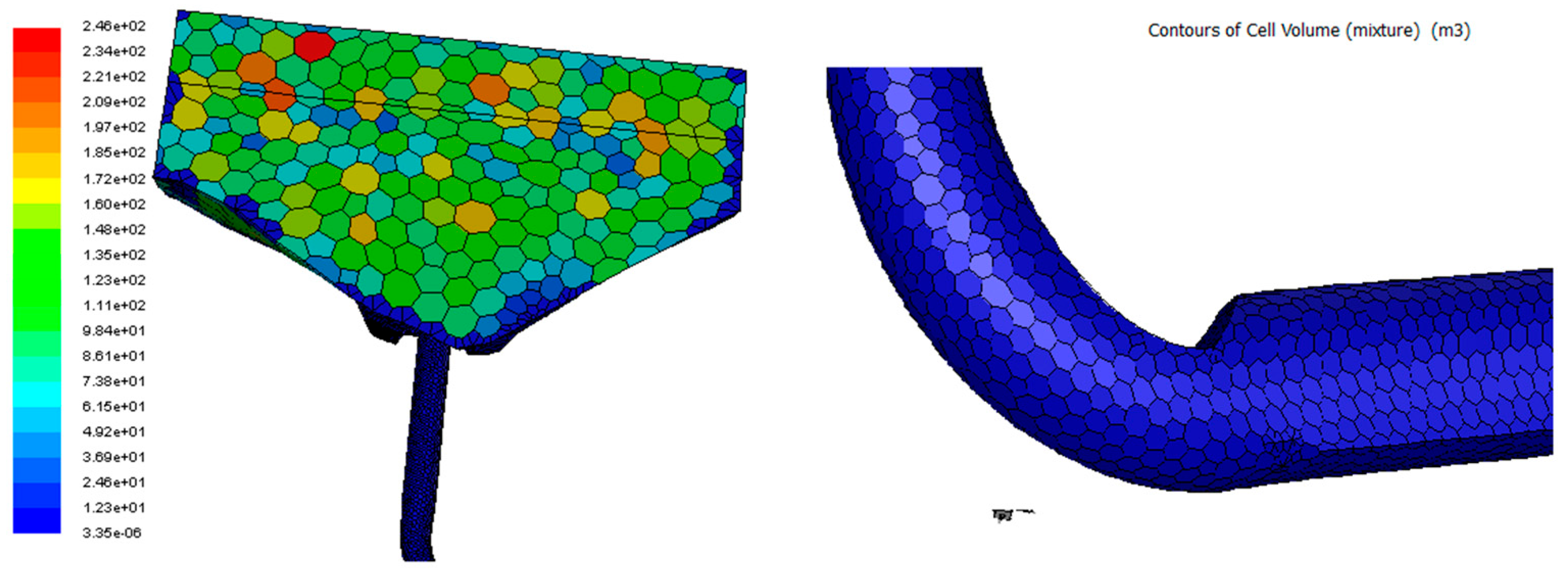
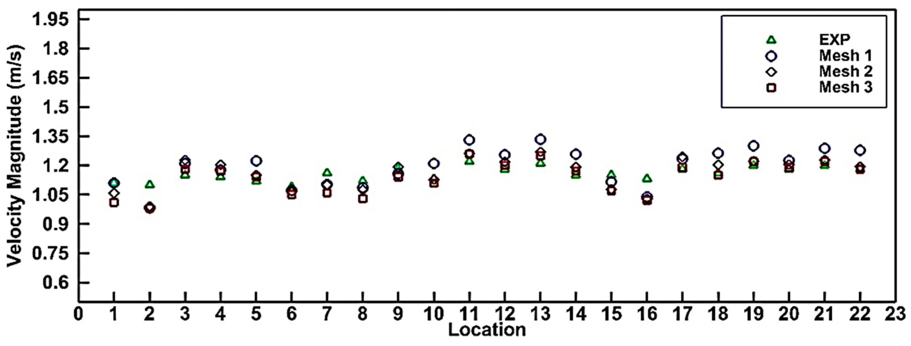
A 3D geometry of the numerical model was drawn in AutoCAD 2022 and meshed in the ANSYS, and then the flow field was meshed by honeycomb networks. The computational domain was discretized using an unstructured grid of honeycomb cells. This type of mesh is particularly effective for complex geometries like the morning-glory spillway, balancing computational efficiency with accuracy. To accurately resolve the near-wall flow, prismatic inflation layers were applied at the boundaries. After solving the problem, the previous network was changed to achieve network independence, and three different models were developed with honeycomb meshes based on the details of Table 2. The honeycomb meshes developed for the numerical model of the morning-glory spillway are illustrated in Figure 1. Velocities on 22 points over the spillway crest were extracted based on Figure 2 for meshing and experimental results. Since the difference between the points was less than 5% for meshes 1 to 3, mesh 1 was selected as the optimal mesh to reduce the computational costs of the analyses and calculations. Boundary conditions and the numerical model’s solution method are shown in Table 3.
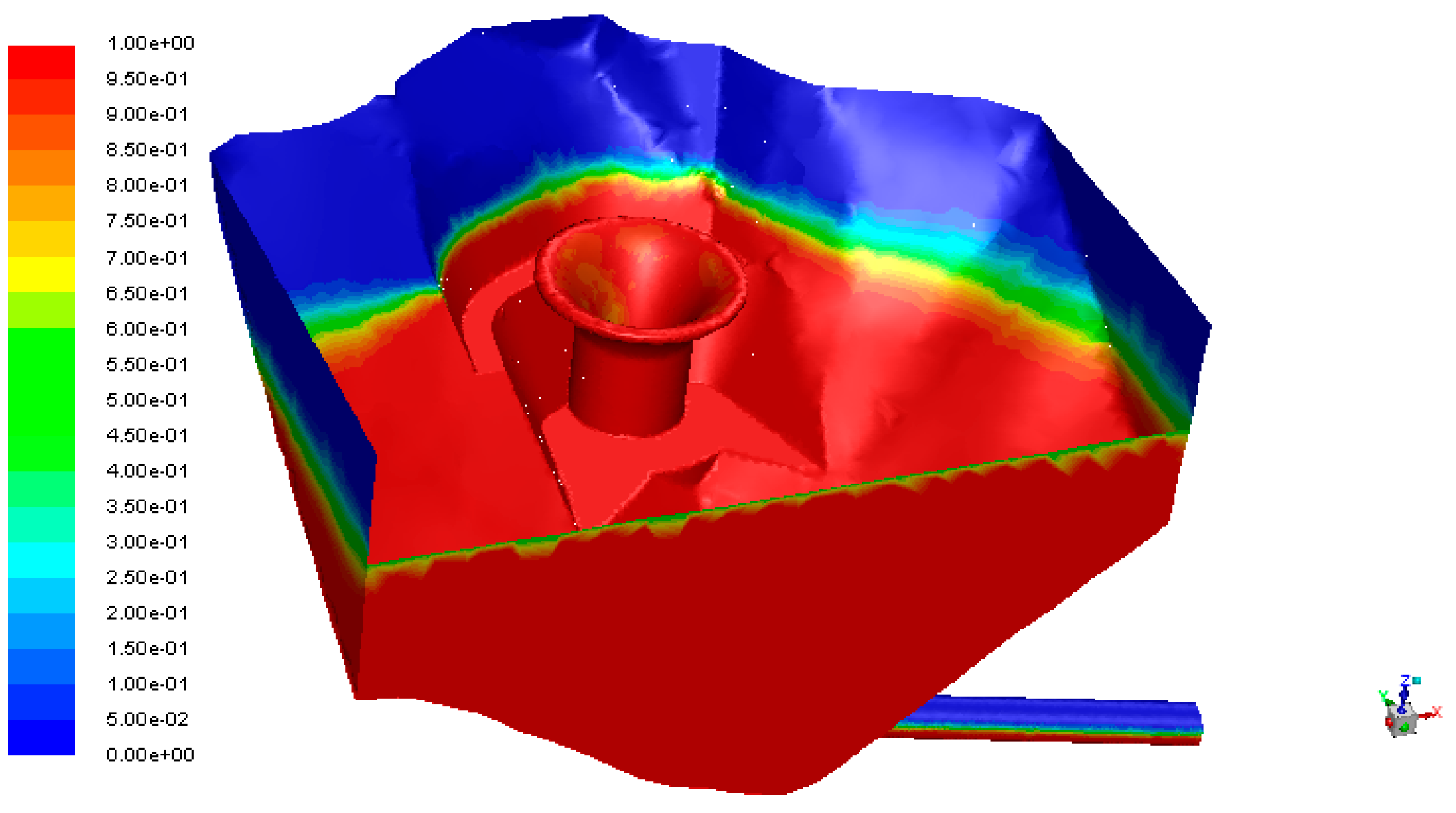
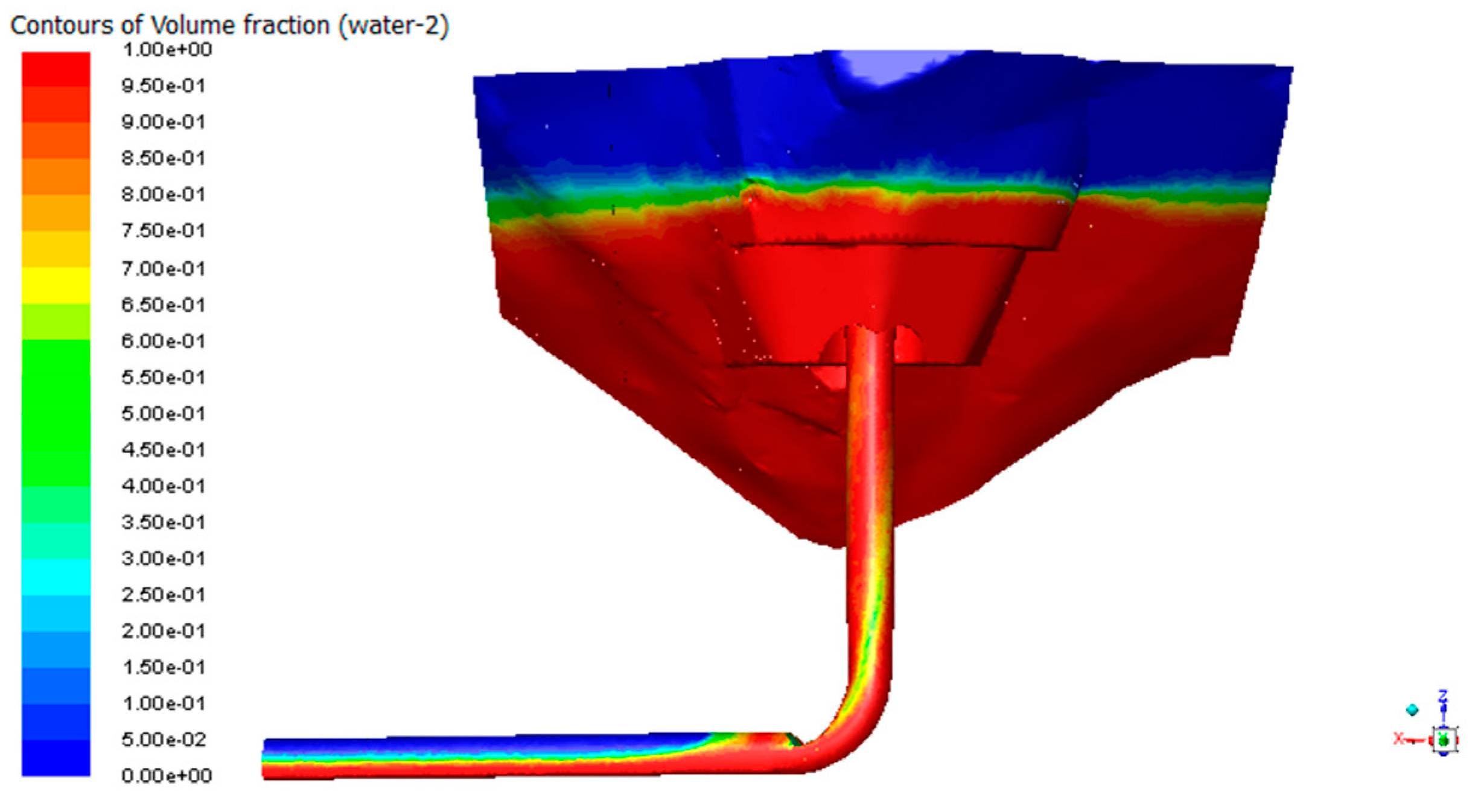
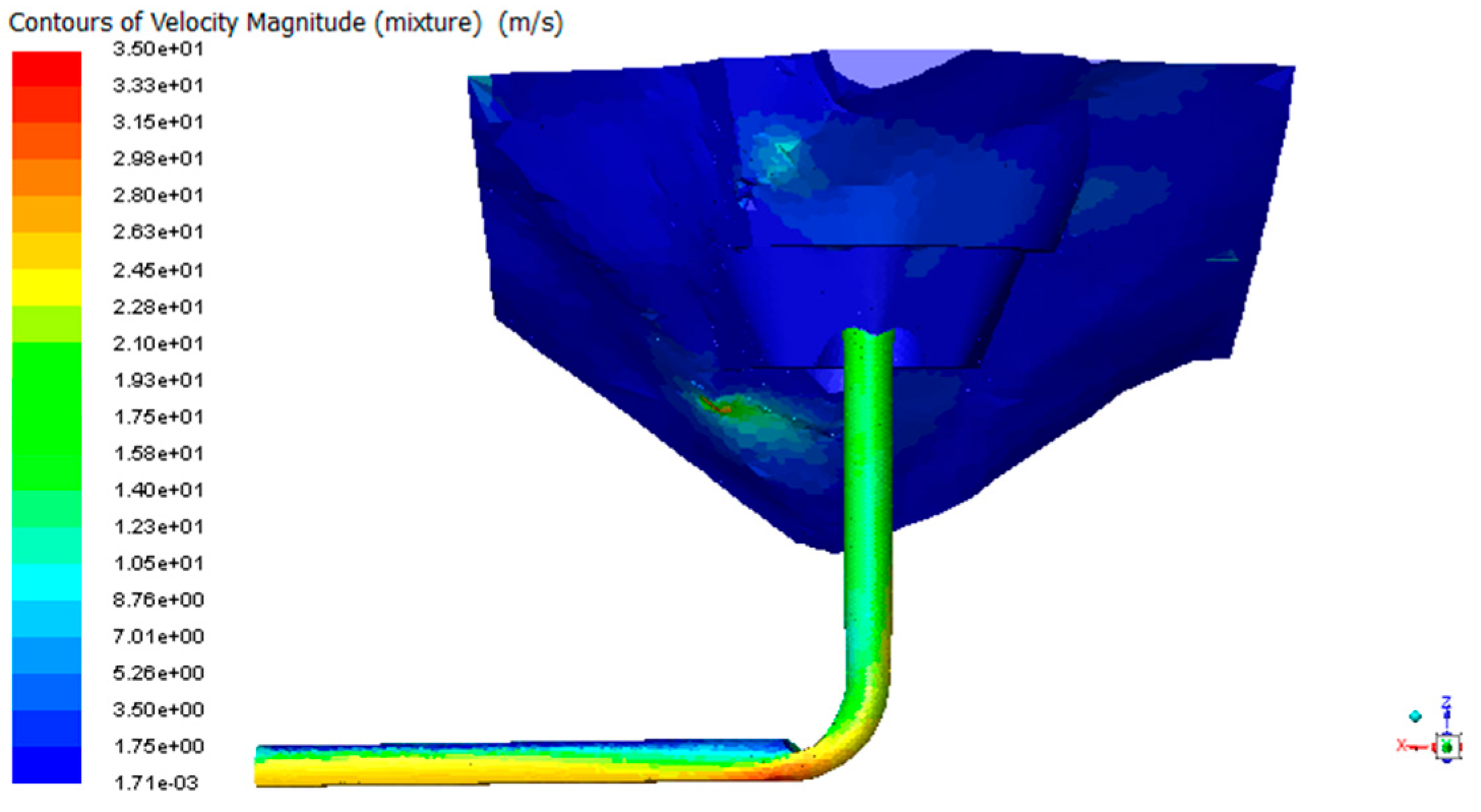
The flow equations were solved for an inflow discharge = 640 m3/s and then the flow became constant after 600 s; overall, solution of the flow equations lasted 850 s. A transient simulation was conducted using adaptive time stepping, with step sizes ranging from 0.001 s to 0.00001 s. Convergence within each step required the scaled residuals for all governing equations to fall below 1 × 10⁻⁴, with a maximum of 20 iterations allowed. The total simulated flow time was 850 s to ensure full development and stability of the cavitating flow. According to the contour of the air–water phases in Figure 3, while the flow control is outflow, the crest, vertical shaft, and knee joint are submerged. The color bar scale from 0 to 1 represents the volume fraction of water. A value of 1.0 (red) indicates a cell completely filled with water, 0.0 (blue) indicates a cell filled with air, and values between 0 and 1 represent cells containing a mixture of both phases. In Figure 4, velocity contour, the highest velocity occurs at the lowest knee-joint point and the velocity in that area is greater than 30 m/s. The velocity values in this validation plot are local measurements at specific points on the spillway transition. The high velocities cited in the results section than 30 m/s correspond to the fully accelerated flow in the downstream shaft and elbow.

2.2. Validating the Results of the Numerical Modeling

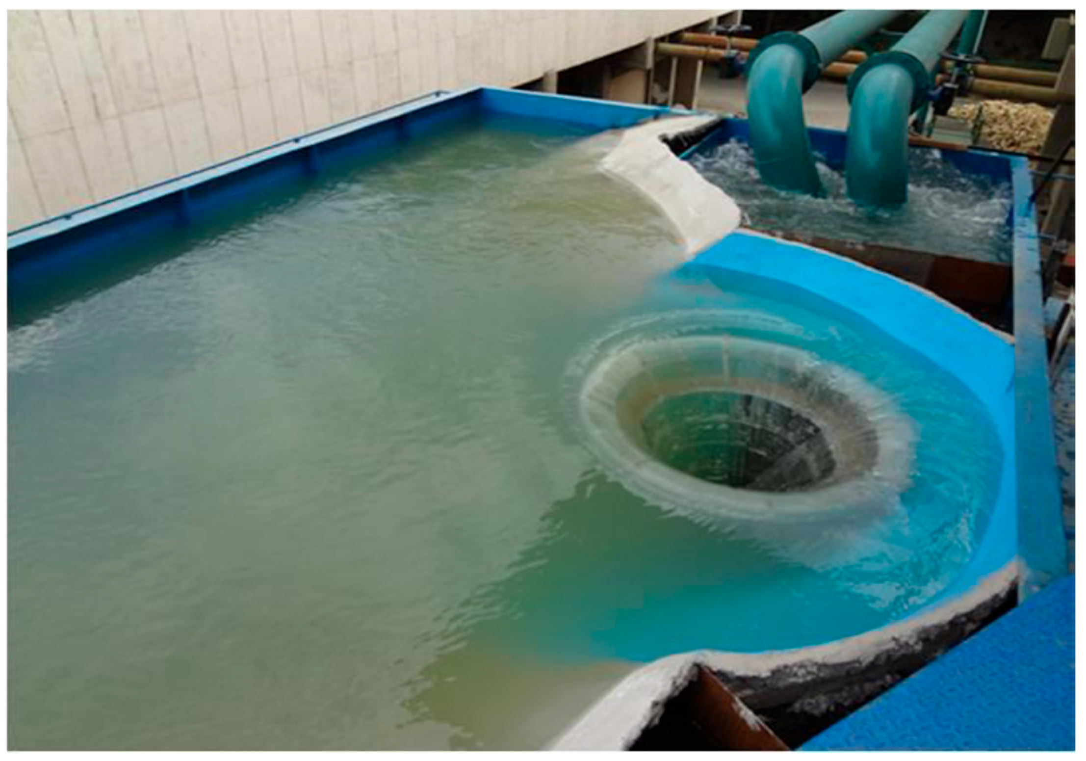
Figure 5 and Figure 6 indicate the 1:30 scale geometry of the numerical and experimental models of the morning-glory spillway of Haraz Dam, the results of both which have been compared for validation purposes (plans were developed in 2018 by the Iran-Water Resource Research Laboratory).
The MAER criterion determines the mean percentage error value as follows (Equation (6)) [33]:
M A E R =   C e C a C e × 100 n
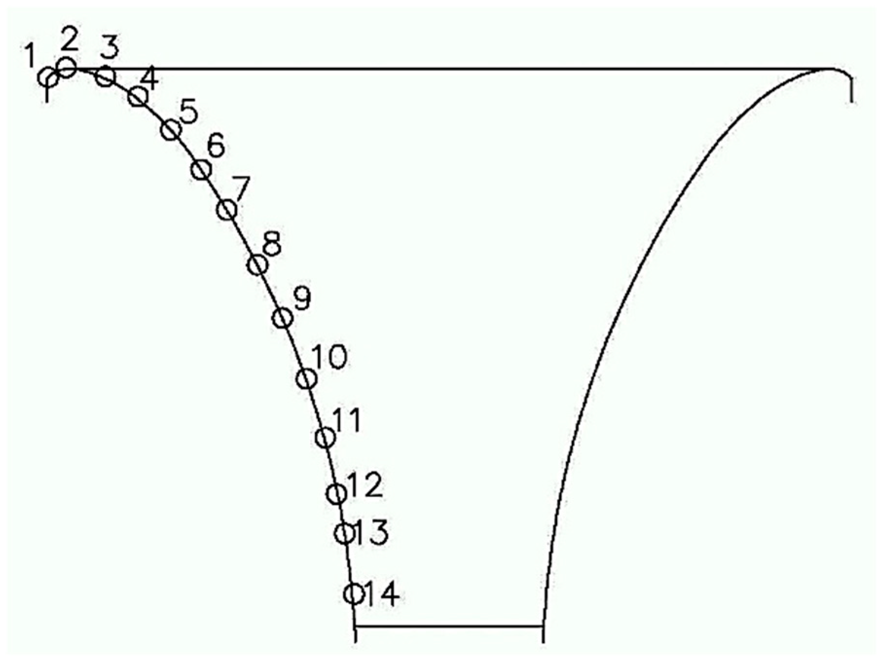
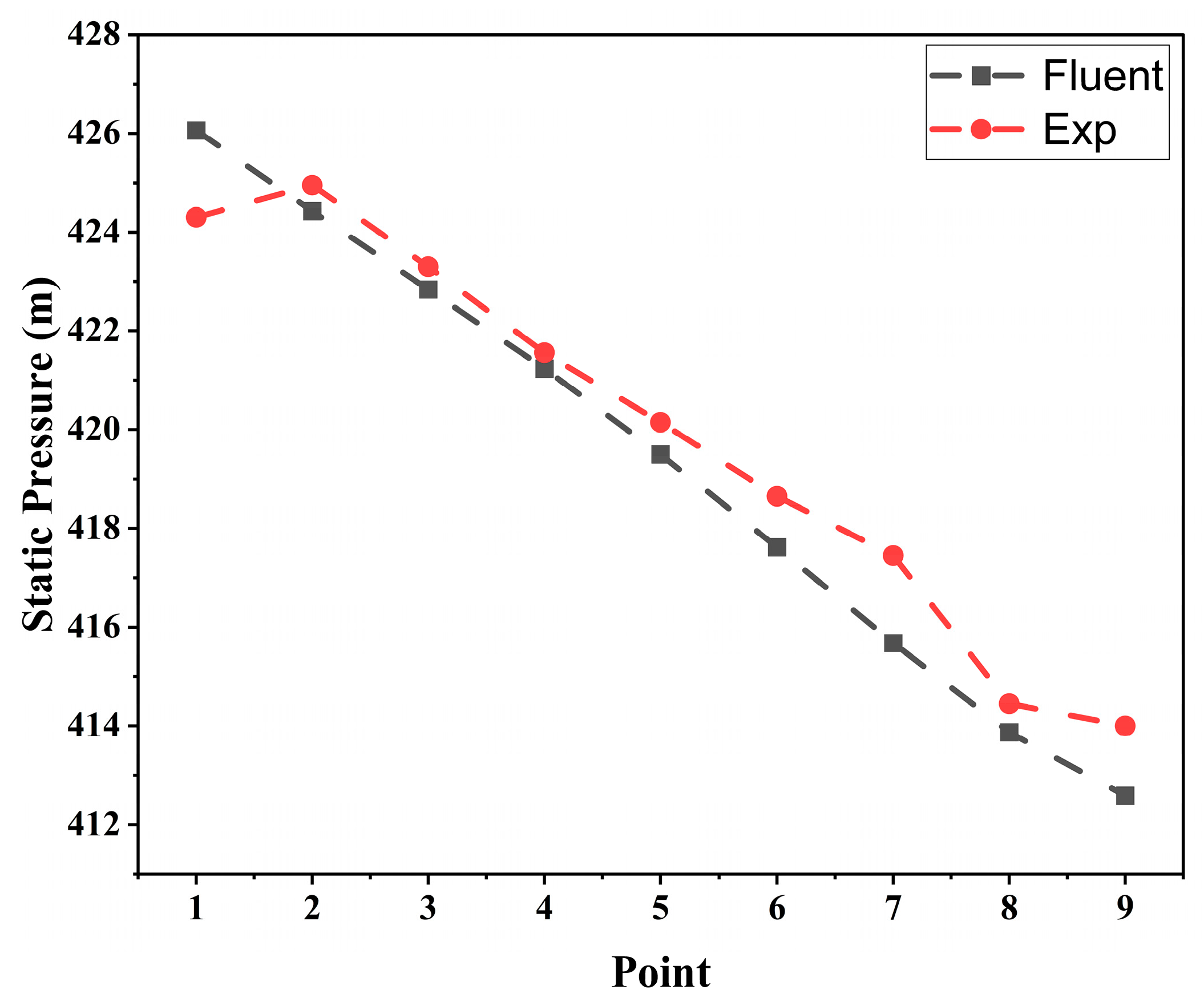
where Ce and Ca are the numerical and experimental results, respectively, and n is the number of data; here, n = 1 because the error values have been extracted independently for each data. Table 4 presents the mean percentage error (MAER) of the velocity and pressure parameters for different parts of the spillway between the numerical and experimental models. As shown, static pressures are not significant compared to the calculated turbulent flow velocity. A calculated MAER of 4.097% indicates the high accuracy of the numerical model. Figure 7 and Figure 8 show the locations of 14 points on the ogee part and the diagram of static pressure (m) between the numerical and experimental models, respectively; in Figure 8, the calculated MAER is 0.28%.

2.3. Problem Uncertainties

Cavitation depends on such factors as the flow velocity and pressure, operation time, spillway surface roughness, and fluid features. Considering the analytical and standard relationships that determine the cavitation index as the performance level, 6 variables, (1) temperature, (2) water density, (3) air density, (4) water vapor pressure, (5) inflow velocity, and (6) absolute spillway surface roughness, were selected as model uncertainties, and analysis of variance (ANOVA) and data distribution normality were examined for them using the Shapiro–Wilk test, where the null hypothesis represents the normal data distribution and the opposite hypothesis indicates the non-normal data distribution. As the hypothesis is rejected for p-values less than the error value, the sample data are not obtained from a normal population. Assuming X1, X2, …, Xn as the observed values of random variable X, the statistic of the Shapiro–Wilk test is defined as follows (Equation (7)) [34]:
W =   ( i = 1 n a i x ( i ) ) 2 i = 1 n ( x i x ¯ ) 2
where vector ai is found as follows (Equation (8)):
a 1 , a 2 , a n = m T V 1 C
where V is the covariance matrix of the order statistics and vector C is defined as follows (Equation (9)):
C = V 1 m = ( m T V 1 V 1 m ) 1 / 2
where vector m is the mathematical expectation of the order statistics and x ¯ is the average value observed from the random samples. The difference between xi and xi is that the former is the value of the random sample and the latter is the order statistic (ordered value) of the random variable. According to Table 5, since temperature, velocity, and absolute roughness-related data are in the same numerical range, they follow a uniform distribution. Statistical analyses related to water/air density and water vapor pressure uncertainties were performed using the Shapiro–Wilk test (Table 6). As the p-values are greater than the model error (0.05), the null hypothesis (normality of data distribution) is not rejected.
In hydraulic engineering problems, since various uncertain variables have their momentary specific conditions and values in different situations, establishing a correlation among them in cavitation responses is difficult because the related assumptions affect the final prediction of the expected responses. The matrix of correlation among dependent uncertainties was extracted as follows (Equation (10)):
1 c o r x 1 , x 2 c o r x 1 , x 3 c o r x 1 , x 4 c o r x 2 , x 1 1 c o r x 2 , x 3 c o r x 2 , x 4 c o r x 3 , x 1 c o r x 3 , x 2 1 c o r x 3 , x 4 c o r x 4 , x 1 c o r x 4 , x 2 c o r x 4 , x 3 1 = 1 0.933 0.911 0.985 0.933 1 0.894 0.729 0.911 0.894 1 0.942 0.985 0.729 0.942 1

2.4. Experiment Design and Simulation

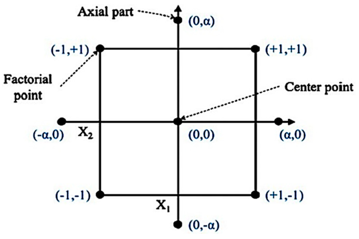
The number of the problem simulations was determined by examining the concept related to different RSMs, which includes three-level full factorial design, Box–Behnken design, and CCD. The latter, used in this research, includes a two-level full or fractional factorial design along with axial and central points (Figure 9), where each factor has 5 levels and factor points are determined as the modeling boundaries by designing an experiment, wherein the upper and lower limits are defined by ±1, negative values in the original are denoted with a hyphen (-).
The total number of experiments is determined by the CCD as follows (Equation (11)):
R u n = 2 f p + 2 f + 1 + r
where f is the number of variables, r is the number of iterations, and p is a fraction of the full factorial design. As the Min-run Res V design reduces the number of analyses when there are more than 5 uncertainty factors, it needed 35 analyses in this research for 6 uncertainty factors and 1 central point; hence, 35 samples were generated by the LHS.
If the cavitation damage-related uncertainties are x = x 1 . x 2 . x 3 . . x 6 , then the mean vector is l n μ x = ( ln μ x 1 . ln μ x 2 . . ln μ x 6 ) , standard deviation vector is   σ L n x = σ L n x 1 . σ L n x 2 . . σ L n x 6 , and the covariance matrix is σ J K = C o v x J . x K ; hence LHS generates a 35 × 6 Z-matrix, and the dependent multivariate random variables are generated as follows (Equation (12)):
Y = l n μ x + L ~ Z
where L ~ is the lower triangular matrix corresponding to the covariance matrix.

2.5. Summary of the Proposed Procedure

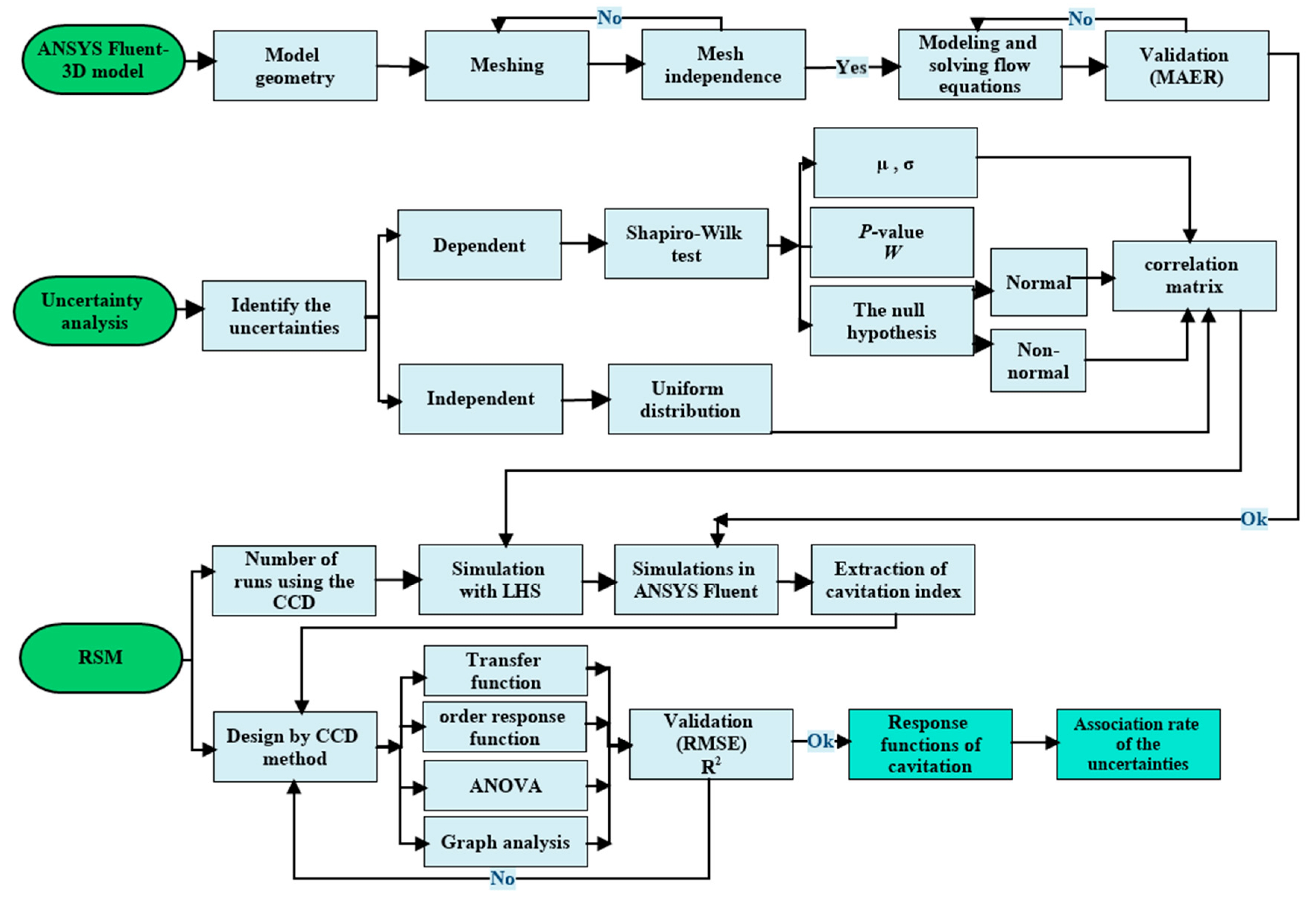
In this research, results of the statistical and cavitation damage functions were extracted to analyze model uncertainties by different methods. Figure 10 shows the flowchart of the general method used to achieve the desired results.

3. Results and Discussion

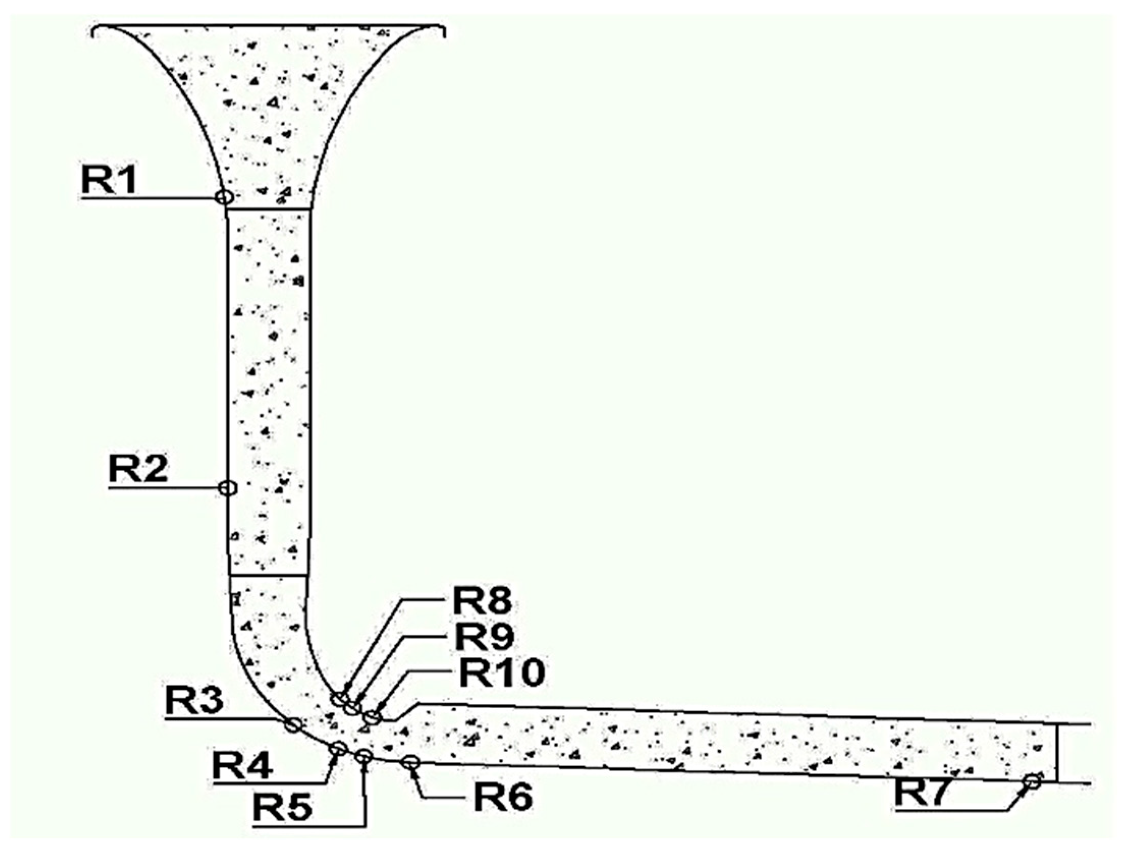
After the LHS generated a 35 × 6 matrix for the cavitation damage, 35 numerical analyses were conducted by a supercomputer processing system, 46 points were evaluated, and 10, with the minimum cavitation number, were selected as the critical points on the morning-glory spillway; 1 on the ogee part, 1 on the vertical shaft, 3 over the knee joint, 3 at the bottom of the knee joint, and 2 at the bottom of the horizontal tunnel. Locations of these points on two spillway dimensions are shown in Figure 11.

3.1. Results of RSM Analysis

Response surface, a function of the responses of each experiment (simulation), is provided as a performance factor. In this study, although the design model is a second-order RSM involving terms related to the effect of the main factors, second-order factors and their interactions, it cannot keep the line of best fit of all the terms. Hence, their significance level is determined by p-values; the intended term is significant if p-values < 0.05 and insignificant in the response if p-values > 0.1. Response normalization is possible through various transformations, and this study used transfer functions for the normality of its 10 final responses. In Table 7 that lists a summary of the design, including uncertainty factors, upper and lower bounds, mean and standard deviation of responses, transfer function, and type of response function, R2 and R3 do not need to be transferred. Out of 10 response functions of cavitation finally extracted at the spillway (Table 8), R1, R4, R5, and R6 are linear, R2 and R3 are inter-variable interaction effects, and R7R10 follow second-order equations.
The criteria used to assess the RSM accuracy were MSE (mean square error), R (correlation coefficient), and RMSE (root mean square error) shown, respectively, by Equations (13)–(15) [35].
M S E = i = 1 n ( y e s t i y o b s i ) 2 n
R = i = 1 n y o b s i y ¯ o b s × y e s t i y ¯ e s t i = 1 n y o b s i y ¯ o b s 2 i = 1 n y e s t i y ¯ e s t 2
R M S E = i = 1 n ( y e s t i y o b s i ) 2 n
where y o b s is the value found from numerical analysis, y ¯ o b s is the related mean value, y e s t is the estimated value, and y ¯ e s t is the related mean value. In Table 9 that lists the values of R, MSE, and RMSE of the results of the numerical and prediction models for 10 responses, MSE < 5%, which is acceptable, and R shows that the coefficient of determination obtained from the second-order equation is much higher than those of the linear equations, concluding that the former predicts the cavitation damage better than the latter.
This study examined the results of the cavitation damage on three spillway points selected from among 10 predicted responses.

3.2. Response at Point R6

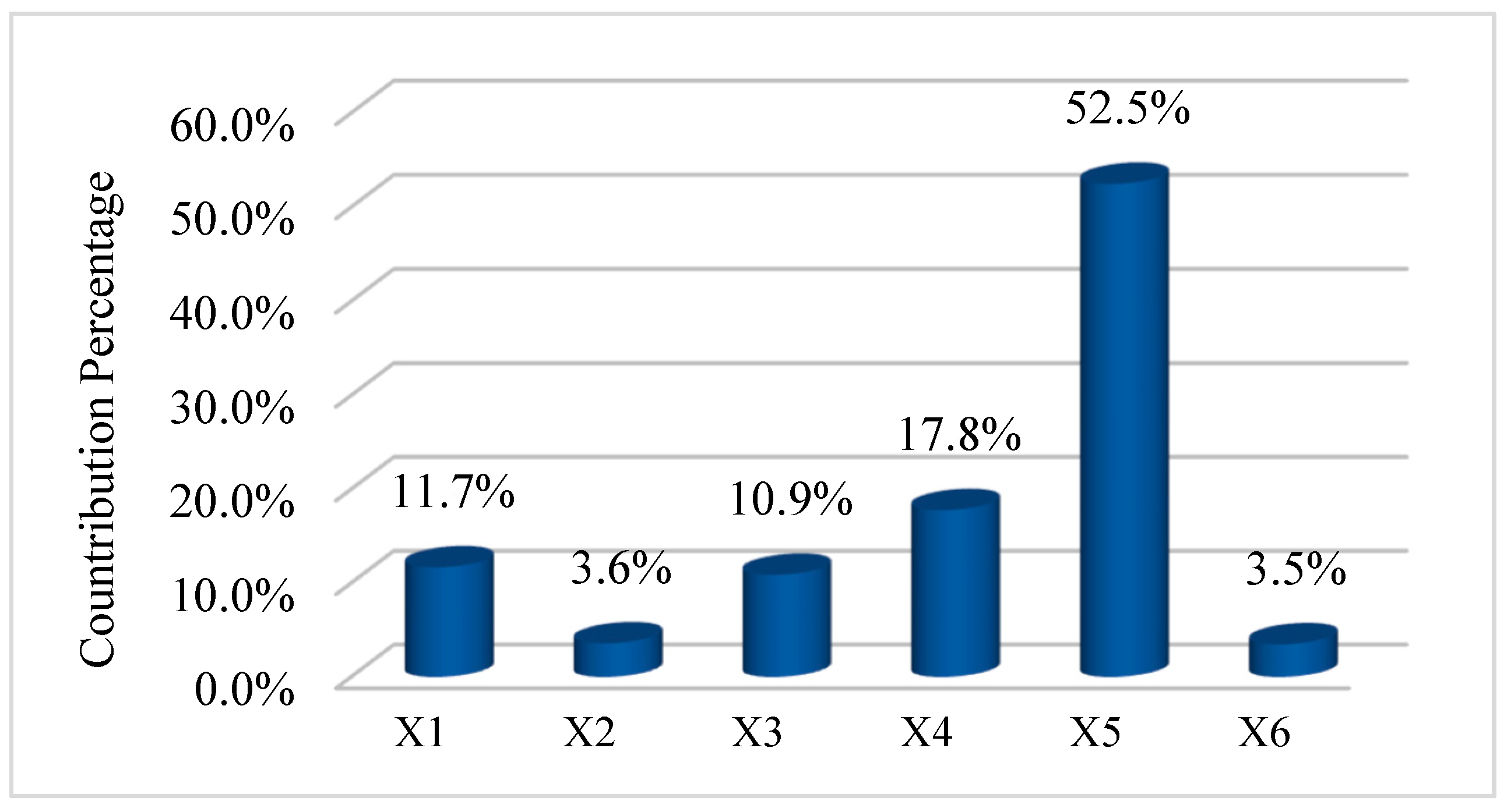
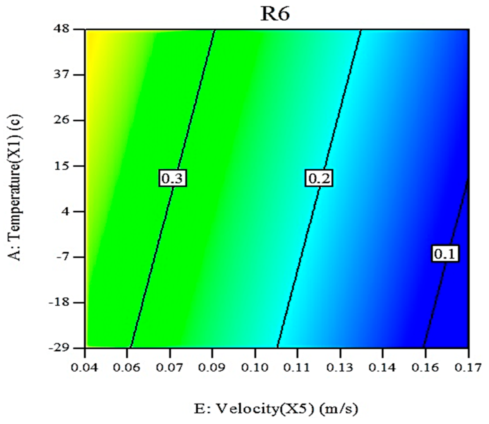
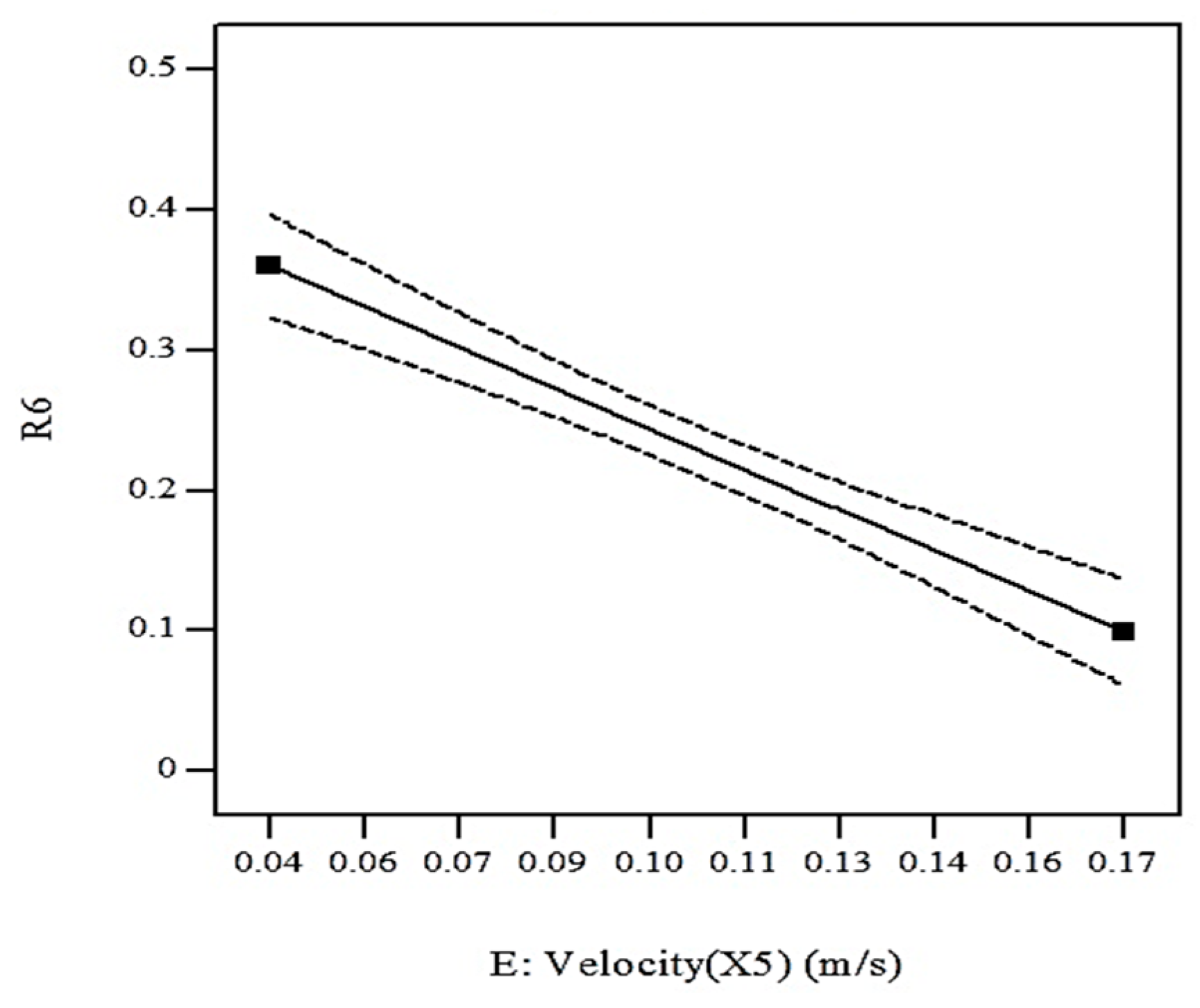
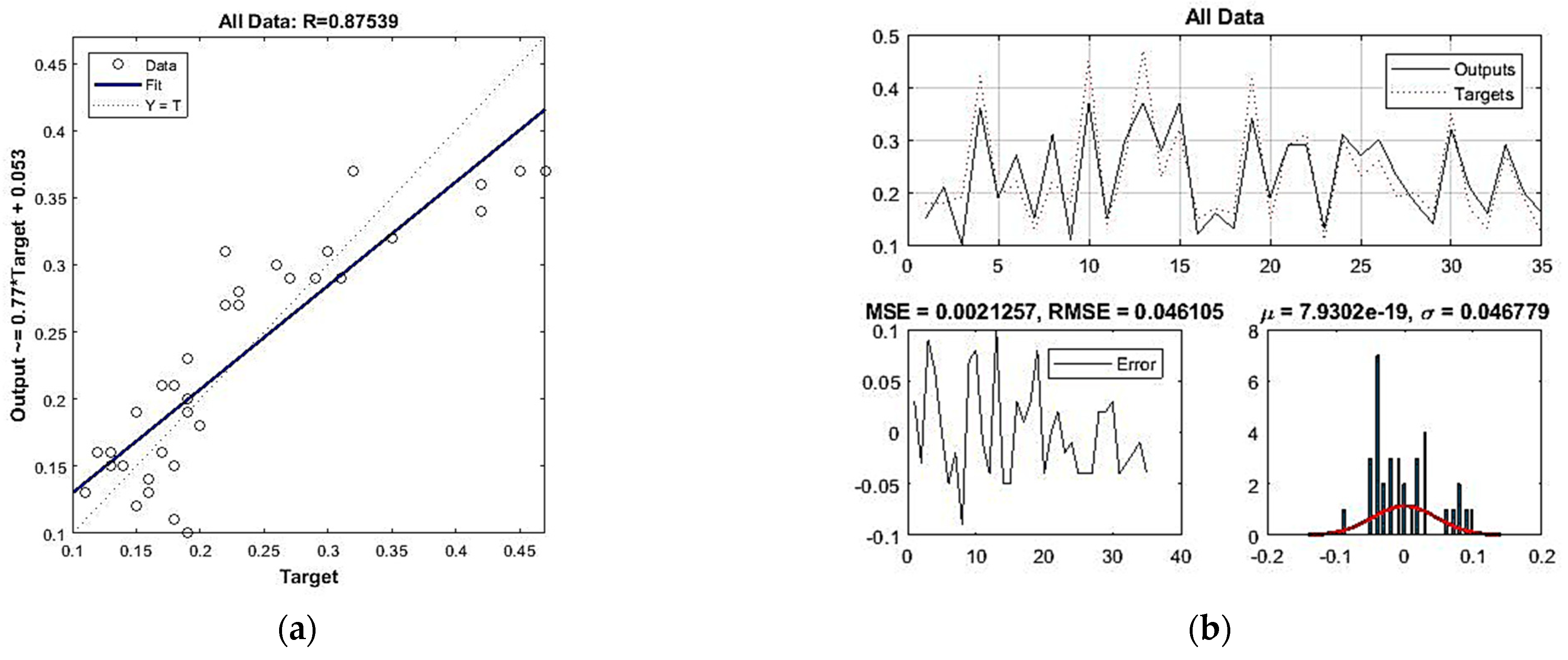
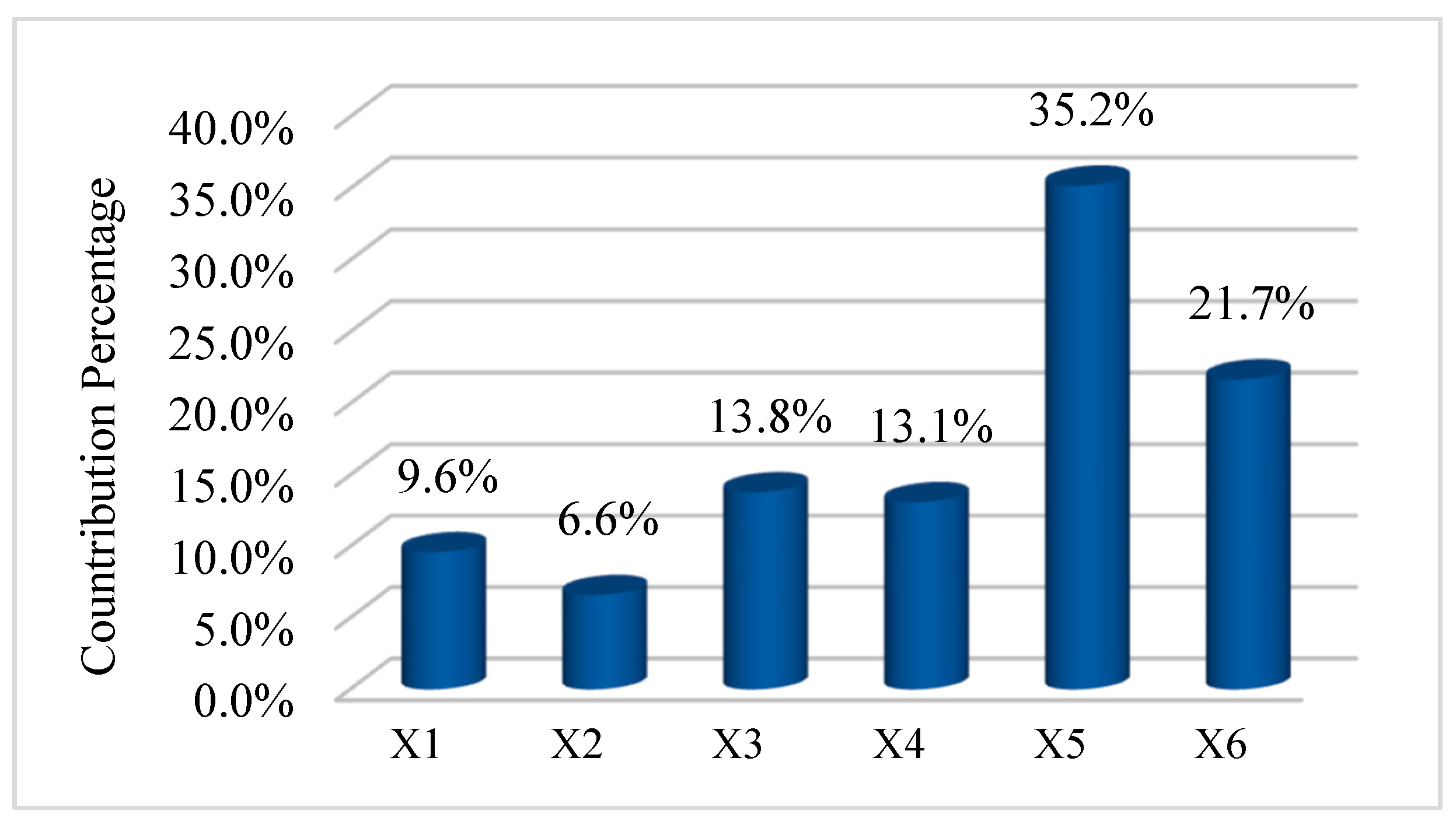
The response function at this point is extracted as a liner. According to Figure 12, the association rate of the model uncertainty factors in this response indicates that the greatest effect is related to the velocity of the inflow to the spillway. Effects of water vapor pressure and temperature are significant in predicting the cavitation damage. The temperature-velocity interaction effects (Figure 13) and those of velocity–cavitation index (Figure 14) reveal that the cavitation response (index) decreases and reaches a critical state when the inflow velocity increase; here, the cavitation damage potential rises. While the sensitivity analysis confirmed inflow velocity as the predominant factor governing cavitation risk (accounting for over 50% of the response variance), the revised analysis also quantifies the secondary role of other parameters. For instance, within the operational range studied, the contribution of water temperature variation to the cavitation index was less than 12%, and the effect of wall roughness remained negligible below a threshold. The error graphs for response R6 are shown in Figure 15, respectively, where part a shows the correlation between the target and output data, and part b corresponds to the target data found from the ANSYS Fluent model, the output data predicted for 35 simulations, MSE, RMSE, histogram, and mean and standard deviation for the cavitation index.

3.3. Response at Point R9

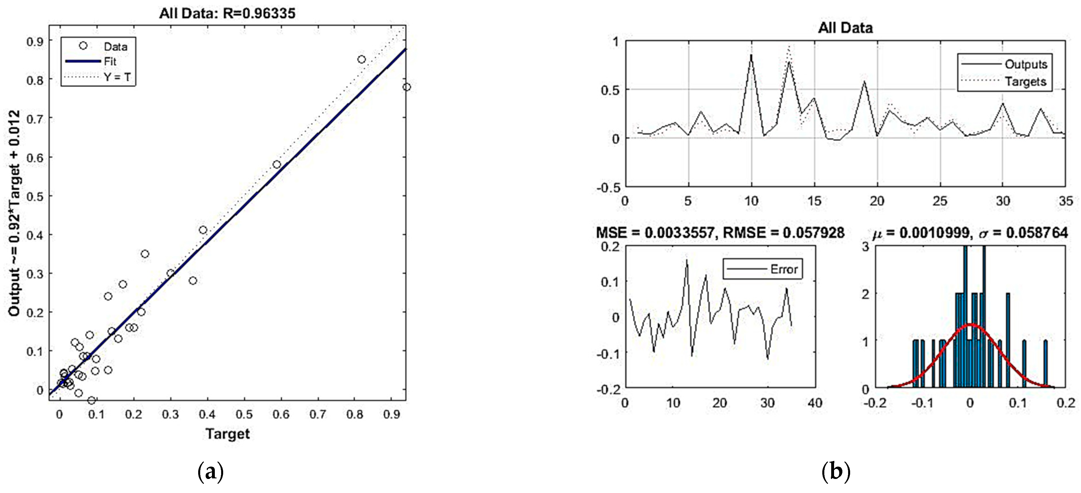
The response function at this point is extracted as a second-order equation. According to Figure 16, the association rate of the model uncertainty factors in this response indicates that the greatest effect is related to the velocity of the inflow to the spillway, and the surface roughness contributes more than 21% in predicting the response. The error graphs for response R9 are shown in Figure 17, respectively, where part a shows the correlation between the target and output data, and part b corresponds to the target data found from the ANSYS Fluent model. The error graph shows the correlation diagram of actual (numerical model) results versus those predicted by RSM with R > 96%.
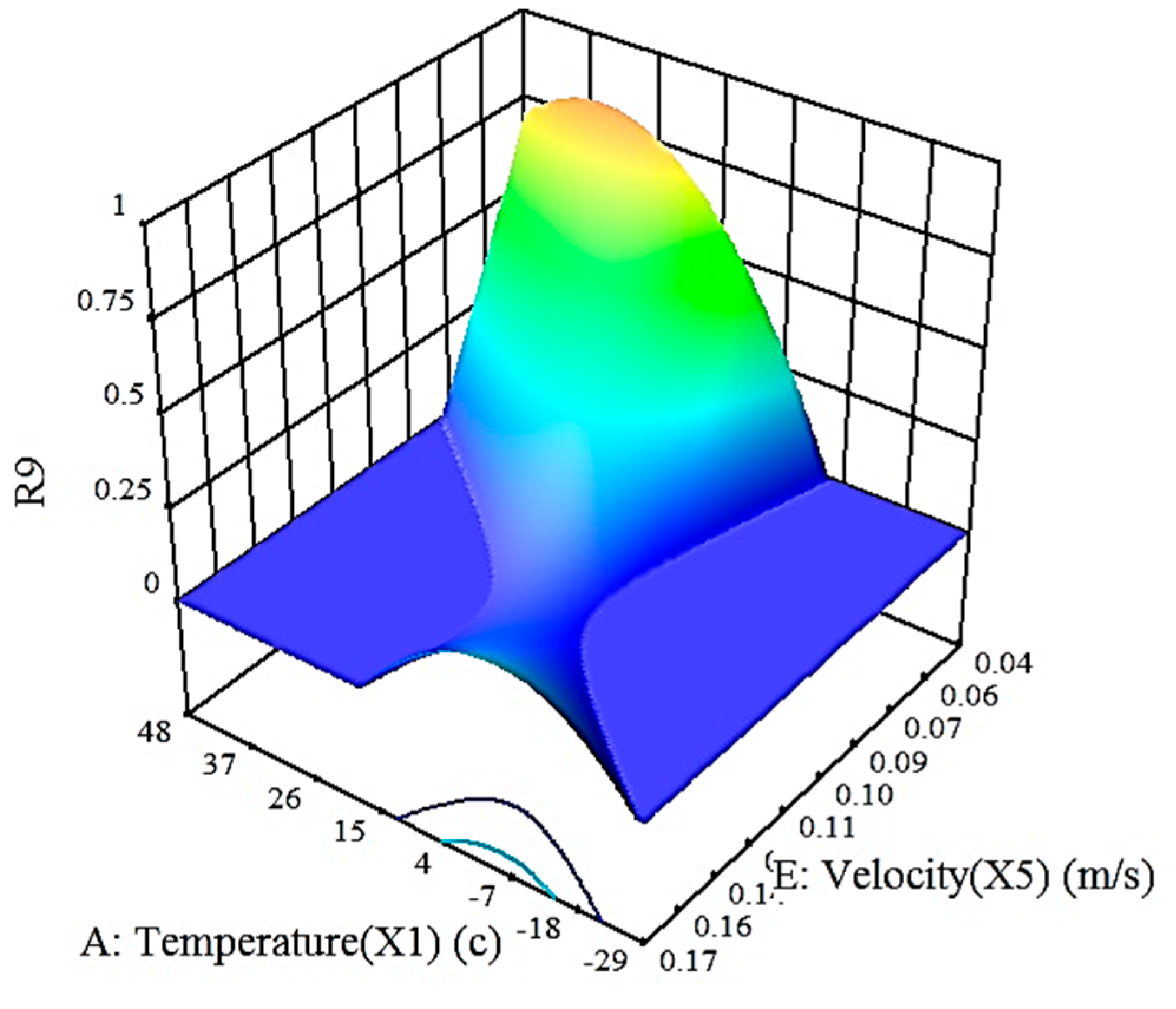
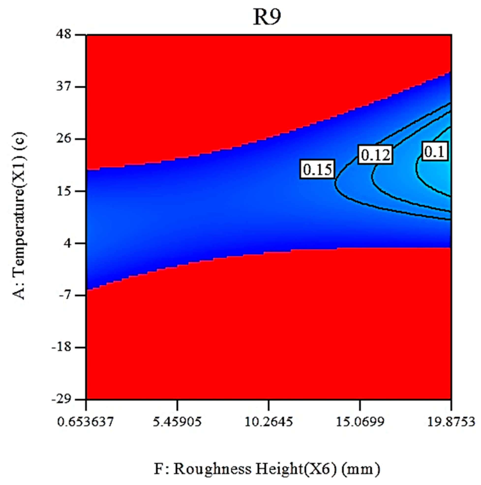
Effects of the temperature–velocity and temperature–surface roughness interactions on R9 are shown in Figure 18 and Figure 19, respectively; as shown in the former, an increase in velocity decreases the cavitation index considerably, causing it to reach a critical state for damage, and in the latter, as the spillway surface roughness increases, the cavitation index decreases with a gentle slope, causing the damage to be more at points where the spillway surface has a higher roughness.

4. Conclusions

This study assessed cavitation responses at various points on the morning-glory spillway of Haraz Dam, Iran, accounting for uncertainties in model parameters. These included time-dependent uncertainties such as water density, air density, and water vapor pressure, as well as independent uncertainties like fluid characteristics, inflow velocity, and absolute surface roughness. The spillway flow field was modeled using ANSYS Fluent 3D, and the numerical results were validated against experimental hydraulic parameters. With a mean absolute error rate (MAER) of less than 5%, the results were deemed acceptable. The correlation matrix for statistical analyses of model uncertainties was derived using the Shapiro–Wilk test.
The flow field was analyzed through 35 LHS numerical simulations, considering inter-correlations among model uncertainties. Cavitation index responses were extracted for 10 critical points. Response functions R1, R4, R5, and R6 were linear, R2 and R3 were interaction effects, and R7 to R10 followed second-order equations. Except for R2 and R3, all responses were transformed via transfer functions to obtain normalized response data. The RMSE between Fluent 3D numerical data and RSM predictions was less than 5%, and the correlation coefficient RR between actual and predicted data indicated reliability. Second-order equation responses were more accurate than linear responses in predicting cavitation damage.
Response assessments showed that the inflow velocity, absolute surface roughness, and water vapor pressure had the highest association rates with model uncertainties. Results demonstrated that increasing inflow velocity reduced the cavitation index while increasing the probability of cavitation damage-induced failure. Similarly, higher absolute surface roughness pushed the cavitation index closer to the critical boundary, raising failure probability. High R values and RMSE < 5% confirm that RSM is a highly accurate method, capable of effectively estimating spillway cavitation damage responses.
The integrated CFD-RSM framework developed herein provides a robust and practical methodology for cavitation risk assessment under uncertainty. While the computational demand of 3D simulations and the site-specific derivation of uncertainty parameters are inherent considerations, the study successfully demonstrates a transferable workflow. The derived response surface functions offer a significant reduction in computational cost for future probabilistic analyses of similar structures.

5. Suggestions for Future Studies

The following suggestions can help improve the model in future research:
  • Utilize optimal values for each expected uncertainty and cavitation damage response results at critical points to mitigate cavitation-related damage.
  • Apply the model responses at the 10 critical points identified in this study to establish relationships between uncertainties, assess reliability, and calculate failure probabilities.
  • Compare the RSM results of this study with alternative prediction methods, such as neural networks (NNs) and fuzzy logic.
  • Use the cavitation damage response functions developed in this research to identify safe zones and prevent spillway failure.

Author Contributions

Conceptualization, M.A.M. and M.R.; Methodology, M.G.; Software, M.G.; Validation, M.G.; Formal analysis, M.G.; Investigation, M.G.; Resources, M.G.; Data curation, M.G.; Writing—original draft, M.G.; Writing—review & editing, M.A.M. and M.R.; Visualization, M.A.M., G.A. and M.R.; Supervision, M.A.M., G.A. and M.R.; Project administration, M.G., M.A.M. and M.R. All authors have read and agreed to the published version of the manuscript.

Funding

This research received no external funding.

Data Availability Statement

The datasets generated during and/or analyzed during the current study are available from the corresponding author on reasonable request.

Conflicts of Interest

The authors declare no conflicts of interest.

References

  1. Foroudi, A.; Barati, R. Experimental study of cavitation index in an ogee spillway by considering convergence angle of sidewalls. Water Supply 2022, 22, 5729–5738. [Google Scholar] [CrossRef] [Scilit]
  2. Aydin, M.C.; Ulu, A.E. Developing and testing a novel pressure-controlled hydraulic profile for siphon-shaft spillways. Flow Meas. Instrum. 2023, 90, 102332. [Google Scholar] [CrossRef] [Scilit]
  3. Falvey, H.T. Cavitation in Chutes and Spillways; US Department of the Interior, Bureau of Reclamation: Washington, DC, USA, 1992. [Google Scholar]
  4. Matos, J.; Novakoski, C.K.; Ferla, R.; Marques, M.G.; Dai Prá, M.; Canellas, A.V.B.; Teixeira, E.D. Extreme pressures and risk of cavitation in steeply sloping stepped spillways of large dams. Water 2022, 14, 306. [Google Scholar] [CrossRef] [Scilit]
  5. Manogaran, T.; Zainol, M.M.A.; Wahab, M.K.A.; Aziz, M.A.; Zahari, N.M. Assessment of flow characteristics along the hydraulic physical model of a dam spillway. J. Civ. Eng. Sci. Technol. 2022, 13, 69–79. [Google Scholar] [CrossRef] [Scilit]
  6. Wuyi, W.; Bin, L.; Awais, R. Numerical prediction and risk analysis of hydraulic cavitation damage in a high-speed-flow spillway. Shock Vib. 2018, 2018, 1817307. [Google Scholar] [CrossRef] [Scilit]
  7. Sharifi, S.N. Enhancing performance of stepped spillways: CFD analysis of shaped step surfaces for improved flow dynamics. Results Eng. 2025, 25, 103704. [Google Scholar] [CrossRef] [Scilit]
  8. Kalateh, F.; Aminvash, E. Numerical investigation of aerator position effects on two-phase flow and hydraulic efficiency in morning glory spillway. Innov. Infrastruct. Solut. 2025, 10, 10. [Google Scholar] [CrossRef] [Scilit]
  9. Reza, G.; Dziedzic, M. An improved conceptual Bayesian model for dam break risk assessment. In Proceedings of the World Environmental and Water Resources Congress, Milwaukee, VI, USA, 19–22 May 2024; pp. 1002–1018. [Google Scholar] [CrossRef] [Scilit]
  10. Enjilzadeh, M.R.; Nohani, E. Numerical modeling of flow field in morning glory spillways and determining rating curve at different flow rates. Civ. Eng. J. 2016, 2, 448–457. [Google Scholar] [CrossRef] [Scilit]
  11. Iqbal, S.; Dissanayaka, K.D.C.R.; Tanaka, N. Numerical modeling and validation of dike-induced water flow dynamics using OpenFOAM. ISH J. Hydraul. Eng. 2024, 30, 559–573. [Google Scholar] [CrossRef] [Scilit]
  12. Bordbar, A.; Mousavi Jahromi, H.; Shafaei Bajestan, M.; Sedghi, H. Step effects investigation on the flow regime and cavitation in stepped morning glory spillways. World Appl. Sci. J. 2010, 10, 1024–1031. [Google Scholar]
  13. Feng, C.; Borgonovo, M.; Hu, Y.; Faes, M.G.; Beer, M. Interval fields for geotechnical engineering uncertainty analysis under limited data. ASCE-ASME J. Risk Uncertain. Eng. Syst. Part A Civ. Eng. 2025, 11, 04025004. [Google Scholar] [CrossRef] [Scilit]
  14. Yen, B.C.; Cheng, S.T.; Melching, C.S. First order reliability analysis. In Handbook of Turbulence; Frost, W., Ed.; Water Resources Publications: Littleton, CO, USA, 1986; pp. 1–36. [Google Scholar]
  15. Yen, B.C.; Tung, Y.K. Reliability and Uncertainty Analyses in Hydraulic Design; ASCE Publications: New York, NY, USA, 1993. [Google Scholar]
  16. Motahari Moghadam, E.; Saeidi, A.; Rouleau, A.; Patarroyo, J. A numerical study on the effect of gate configuration on the hydraulic parameters of dam spillways. Results Eng. 2025, 25, 104446. [Google Scholar] [CrossRef] [Scilit]
  17. Zhou, B.; Liu, H.; Zhang, G.; Han, X.; Wang, X.; Tan, S.K. Numerical simulation of cavity dynamics and motion characteristics for water entry of a hydrophobic sphere at various speeds and angles. J. Eng. Mech. 2020, 146, 04020091. [Google Scholar] [CrossRef] [Scilit]
  18. Mozaffari, S.; Amini, E.; Mehdipour, H.; Neshat, M. Flow discharge prediction study using a CFD-based numerical model and gene expression programming. Water 2022, 14, 650. [Google Scholar] [CrossRef] [Scilit]
  19. Kocaer, Ö.; Yarar, A. Experimental and numerical investigation of flow over ogee spillway. Water Resour. Manag. 2020, 34, 3949–3965. [Google Scholar] [CrossRef] [Scilit]
  20. Achintya, H. Recent Developments in Reliability-Based Civil Engineering; World Scientific: Singapore, 2006. [Google Scholar] [CrossRef]
  21. Deng, J.; Gu, D.; Li, X.; Yue, Z.Q. Structural reliability analysis for implicit performance functions using artificial neural network. Struct. Saf. 2005, 27, 25–48. [Google Scholar] [CrossRef] [Scilit]
  22. Ugurhan, B.; Baker, J.W.; Deierlein, G.G. Uncertainty estimation in seismic collapse assessment of modern reinforced concrete moment frame buildings. In Proceedings of the 10th National Conference on Earthquake Engineering, Anchorage, AK, USA, 21–25 July 2014. [Google Scholar]
  23. Azhdary Moghaddam, M.; Hasanalipour Shahrabadi, A. Assessing the reliability of cavitation on chute spillway by using form and Monte Carlo simulation method. Iran. J. Irrig. Sci. 2020, 43, 87–99. [Google Scholar] [CrossRef] [Scilit]
  24. Beheshti-Aval, S.B.; Khojastehfar, E.; Noori, M.; Zolfaghari, M. A comprehensive collapse fragility assessment of moment resisting steel frames considering various sources of uncertainties. Can. J. Civ. Eng. 2016, 43, 118–131. [Google Scholar] [CrossRef] [Scilit]
  25. Khojastehfar, E.; Beheshti-Aval, S.B.; Zolfaghari, M.R.; Nasrollahzade, K. Collapse fragility curve development using Monte Carlo simulation and artificial neural network. Proc. Inst. Mech. Eng. Part O J. Risk Reliab. 2014, 228, 301–312. [Google Scholar] [CrossRef] [Scilit]
  26. Keshtegar, B.; Allawi, M.F.; Afan, H.A.; El-Shafie, A. Optimized river stream-flow forecasting model utilizing high-order response surface method. Water Resour. Manag. 2016, 30, 3899–3914. [Google Scholar] [CrossRef] [Scilit]
  27. Bayari, M.A.; Shabakhty, N.; Izadi Zaman Abadi, E. Estimating collapse risk and reliability of concrete moment frame structure using response surface method and hybrid of artificial neural network with particle swarm optimization algorithm. Proc. Inst. Mech. Eng. Part O J. Risk Reliab. 2021, 235, 1072–1089. [Google Scholar] [CrossRef] [Scilit]
  28. Yang, M.Z.; Wu, Q.X.; Lu, J. Reliability analysis of arch dam considering temperature change field. Appl. Mech. Mater. 2012, 226–228, 1332–1337. [Google Scholar] [CrossRef] [Scilit]
  29. Hameed, M.M.; Al Omar, M.K.; Baniya, W.J.; Al Saadi, M.A. Prediction of high-strength concrete: High-order response surface methodology modeling approach. Eng. Comput. 2022, 38, 1655–1668. [Google Scholar] [CrossRef] [Scilit]
  30. Zhang, H.; Chen, J.; Kou, Q.J.; Pei, L.; Huang, H. A fast prediction method for stability safety and reliability of reservoir bank rock slopes based on deformation monitoring data. Front. Earth Sci. 2022, 10, 944299. [Google Scholar] [CrossRef] [Scilit]
  31. Ministry of Energy; Khorasani Zadeh, A.; Roshan, R. Final Report of Hydraulic Model Studies of the Morning Glory Spillway of Haraz Dam; Project Code: HSM-9202; Iranian Water Research Institute: Tehran, Iran, 2018. [Google Scholar]
  32. Fattor, C.A.; Bacchiega, J.D. Design conditions for morning-glory spillways: Application to Potrerillos Dam spillway. In Advances in Water Resources and Hydraulic Engineering; Zhang, C., Tang, H., Eds.; Springer: Berlin/Heidelberg, Germany, 2009; pp. 2123–2128. [Google Scholar] [CrossRef] [Scilit]
  33. Boes, R.M.; Hager, W.H. Hydraulic design of stepped spillways. J. Hydraul. Eng. 2003, 129, 671–679. [Google Scholar] [CrossRef] [Scilit]
  34. González-Estrada, E.; Villaseñor, J.A.; Acosta-Pech, R. Shapiro-Wilk test for multivariate skew-normality. Comput. Stat. 2022, 37, 1985–2001. [Google Scholar] [CrossRef] [Scilit]
  35. Myers, R.H.; Montgomery, D.C.; Anderson-Cook, C.M. Response Surface Methodology: Process and Product Optimization Using Designed Experiments, 4th ed.; John Wiley & Sons: Hoboken, NJ, USA, 2016. [Google Scholar]
Figure 1. An illustration of honeycomb meshes of the numerical model.
Modelling 07 00078 g001
Figure 2. A comparison of the results of the numerical model velocity for 3 network and experimental models.
Modelling 07 00078 g002
Figure 3. Contour of air–water phases.
Modelling 07 00078 g003
Figure 4. Velocity contour of the flow field.
Modelling 07 00078 g004
Figure 5. Geometry of the Numerical model.
Modelling 07 00078 g005
Figure 6. The experimental model of the spillway.
Modelling 07 00078 g006
Figure 7. The location of 14 points on the ogee part.
Modelling 07 00078 g007
Figure 8. The diagram of static pressure (m) between the numerical and experimental models on the ogee part.
Modelling 07 00078 g008
Figure 9. Factorial, central, and axial points in the CCD [27].
Modelling 07 00078 g009
Figure 10. Flowchart general method of research. The different colors are used to distinguish between the various input cases, output responses, and methodological approaches compared in this analysis.
Modelling 07 00078 g010
Figure 11. The location of 10 critical points on the morning glory spillway of Haraz Dam. The background color enhances the visual clarity and distinction of the data series/methodologies presented in this figure.
Modelling 07 00078 g011
Figure 12. The association rate of R6 uncertainties.
Modelling 07 00078 g012
Figure 13. Interaction effects of temperature and velocity on response R6.
Modelling 07 00078 g013
Figure 14. Interaction effect of velocity on response R6. The different line styles (and the square marker) are used for visual distinction, but the key result is the consistent negative slope across all cases, indicating a uniform trend.
Modelling 07 00078 g014
Figure 15. (a) Correlation between the target and output data for response R6. (b) Target data, output data, error values, and error histogram for response R6. The red line represents the standard normal distribution curve (or the theoretical/expected distribution).
Modelling 07 00078 g015
Figure 16. Association rate of the uncertainties related to response R9.
Modelling 07 00078 g016
Figure 17. (a) Correlation between the target and output data for response R9. (b) Target data, output data, error values, and error histogram for response R9.
Modelling 07 00078 g017
Figure 18. The diagram of the interaction effect of temperature and velocity on the response R9.
Modelling 07 00078 g018
Figure 19. The interaction effect of temperature and absolute roughness on response R9.
Modelling 07 00078 g019
Table 1. The characteristics of the morning glory spillway of Haraz Dam [31].
IndexAmounts
Coordinates of the spillway centerx = 622,982.08, y = 4,012,945.72
1000-year return period discharge305 m3/s
10,000-year return424 m3/s
Maximum possibility of flooding1050 m3/s
Dam threshold levelAltitude 508 m
Spillway threshold levelAltitude 502 m
Table 2. The results of three models obtained from meshing the flow field.
MeshCells NumberPoints NumberNetwork Volume (m3)Element Number
Mesh 192,161473,498min2.8 × 10−6579,499
max3.8 × 102
Mesh 2175,822823,357min2.2 × 10−6957,635
max3.5 × 102
Mesh 3355,2411,542,551min1.95 × 10−61,768,938
max3.1 × 102
Table 3. The boundary conditions and a method for solving numerical model.
IndexMethod
Inlet boundary conditionsVelocity Inlet
Outlet boundary conditionsPressure Outlet
Flow phasesAir–Water, two-phase
Mixed modelVOF
Volume fraction equationsImplicit
Initial phaseAir
Method for solving flow equationsPressure–Velocity Coupling
Method for solving turbulence equationsSecond-order
Table 4. The mean percentage error (MPE) of the numerical and experimental models.
ValidationVelocity over the CrestStatic Pressure in the Ogee PartStatic Pressure on the Vertical ShaftStatic Pressure Above the ElbowStatic Pressure in Horizontal TunnelVelocity in Horizontal Tunnel
Points number22148966
MAER (%)4.0970.2820.1910.2520.1112.762
Table 5. Uncertainties characteristics with uniform distribution.
UncertaintyNameUnitRangeDistribution FunctionVariable Type
X1TemperatureC−30 ≤ X1 ≤ 50UniformDependent
X5Velocitym/s0.04 ≤ X5 ≤ 0.17UniformIndependent
X6Absolute roughnessmm0.1 ≤ X6 ≤ 20UniformIndependent
Table 6. Uncertainties characteristics with normal distribution.
UncertaintyNameUnitShapiro–Wilk ValuesDistributionStatistical ValuesVariable Type
Wp-ValueMeanStandard Deviation
X2Water densitykg/m30.9790.071Normalμ = 996.58σ = 3.191Dependent
X3Air densitykg/m30.9820.119Normalμ = 1.386σ = 0.166Dependent
X4Vapor pressurepa0.9810.104Normalμ = 2986.41σ = 766.36Dependent
Table 7. A summary of design based on the response surface method.
ResponseMinMaximumMeanStd. Dev.RatioTransModel
R10.1183.421.8160.82028.904PowerLinear
R20.6493.551.2450.7125.466None2FI
R30.8752.2311.2750.3012.550None2FI
R40.6331.3280.9550.2072.097PowerLinear
R50.5461.0870.8050.1681.989PowerLinear
R60.1080.4680.2310.0974.307PowerLinear
R70.2211.2160.4390.1995.502PowerQuadratic
R80.0512.0440.3450.43140.082PowerQuadratic
R90.00250.9350.1670.218368.117PowerQuadratic
R100.00090.7180.1340.169765.0PowerQuadratic
Table 8. Response functions of cavitation at the 10 critical points of the morning-glory spillway of Haraz Dam.
Cavitation ResponseResponse Function
R1 R 1 = 4.92 × 10 3 X 1 + 0.01 X 2 0.07 X 3 ( 6.04 × 10 5 ) X 4 + 20.9 X 5 + 0.01 X 6 16.05
R2 R 2 = 2089.07 1.94 X 1 2.1 X 2 1875.95 X 3 + 0.18 X 4 + 557.02 X 5 6.67 X 6 + ( 1.73 × 10 3 ) X 1 X 2        + 0.14 X 1 X 3 ( 1.79 × 10 6 ) X 1 X 4 + 0.16 X 1 X 5 ( 2.62 × 10 3 ) X 1 X 6 + 1.8 X 2 X 3        ( 1.8 × 10 4 ) X 2 X 4 0.58 X 2 X 5 + ( 7.7 × 10 3 ) X 2 X 6 ( 1.55 × 10 3 ) X 3 X 4 + 14.6 X 3 X 5        0.48 X 3 X 6 ( 1.07 × 10 3 ) E X 4 X 5 ( 6.7 × 10 5 ) X 4 X 6 0.74 X 5 X 6
R3 R 3 = 707.7 + 0.05 X 1 0.7 X 2 651.8 X 3 + 0.03 X 4 + 686.6 X 5 + 7.58 X 6 ( 5.22 × 10 5 ) X 1 X 2 + 0.03 X 1 X 3        ( 7.3 × 10 6 ) X 1 X 4 0.07 X 1 X 5 ( 2.72 × 10 3 ) X 1 X 6 + 0.6 X 2 X 3 ( 3.27 × 10 5 ) X 2 X 4        0.72 X 2 X 5 ( 7.18 × 10 3 ) X 2 X 6 ( 1.2 × 10 3 ) X 3 X 4 + 20.62 X 3 X 5 0.35 X 3 X 6        + ( 7.59 × 10 4 ) X 4 X 5 + ( 3.38 × 10 5 ) X 4 X 6 + 0.023 X 5 X 6
R4 R 4 = 9.87 + 2.28 × 10 3 X 1 8.93 × 10 3 X 2 + 0.32 X 3 1.12 × 10 4 X 4 2.38 X 5 + 9.46 × 10 3 X 6
R5 R 5 = 5.18 + 2.8 × 10 3 X 1 4.5 × 10 3 X 2 + 0.4 X 3 1.05 × 10 4 X 4 2 X 5 + 7 × 10 3 X 6
R6 R 6 = 1.68 + ( 7.46 × 10 4 ) X 1 ( 1.27 × 10 3 ) X 2 + 0.07 X 3 ( 2.62 × 10 5 ) X 4 2.08 X 5 + ( 8.9 × 10 4 ) X 6
R7 R 7 = 12449.8 1.75 X 1 24.95 X 2 + 98.37 X 3 + 0.03 X 4 1438.47 X 5 7.73 X 6 + 1.89 × 10 3 X 1 X 2        0.1 X 1 X 3 3.63 × 10 6 X 1 X 4 + 0.21 X 1 X 5 + 8.31 × 10 4 X 1 X 6 0.08 X 2 X 3        3.09 × 10 5 X 2 X 4 + 1.4 X 2 X 5 + 8.83 × 10 3 X 2 X 6 5.93 × 10 4 X 3 X 4 + 14.6 X 3 X 5        0.01 X 3 X 6 4.08 × 10 3 X 4 X 5 2.29 × 10 5 X 4 X 6 + 0.32 X 5 X 6 1.59 × 10 4 X 1 2        + 0.01 X 2 2 5.79 X 3 2 + 1.47 × 10 7 X 4 2 + 80.03 X 5 2 ( 1.16 × 10 3 ) X 6 2
R8 R 8 = 36894.95 + 12.46 X 1 + 72.9 X 2 + 984.27 X 3 0.23 X 4 + 2052.96 X 5 + 2.064 X 6 0.012 X 1 X 2        + 0.06 X 1 X 3 + ( 4.32 × 10 5 ) X 1 X 4 0.66 X 1 X 5 + ( 1.49 × 10 3 ) X 1 X 6 1.016 X 2 X 3        + ( 2.32 × 10 4 ) X 2 X 4 2.005 X 2 X 5 ( 2.46 × 10 3 ) X 2 X 6 + ( 3.81 × 10 3 ) X 3 X 4        62.97 X 3 X 5 + 0.27 X 3 X 6 + ( 7.8 × 10 3 ) X 4 X 5 ( 8.43 × 10 6 ) X 4 X 6 0.09 X 5 X 6        ( 5.12 × 10 4 ) X 1 2 0.03 X 2 2 + 8.11 X 3 2 ( 4.69 × 10 7 ) X 4 2 + 52.85 X 5 2        + ( 1.91 × 10 3 ) X 6 2
R9 R 9 = 21643.43 + 7.93 X 1 + 42.8 X 2 + 627.86 X 3 0.15 X 4 + 1241.94 X 5 + 1.015 X 6 ( 7.95 × 10 3 ) X 1 X 2        0.01 X 1 X 3 + ( 2.14 × 10 5 ) X 1 X 4 0.32 X 1 X 5 + ( 7.91 × 10 4 ) X 1 X 6 0.63 X 2 X 3        + ( 1.55 × 10 4 ) X 2 X 4 1.24 X 2 X 5 ( 1.2 × 10 3 ) X 2 X 6 + ( 1.3 × 10 3 ) X 3 X 4 22.47 X 3 X 5        + 0.11 X 3 X 6 + ( 4.33 × 10 3 ) X 4 X 5 + ( 1.49 × 10 6 ) X 4 X 6 + 0.01 X 5 X 6 ( 5.13 × 10 4 ) X 1 2        0.021 X 2 2 + 2.73 X 3 2 ( 2.18 × 10 7 ) X 4 2 + 64.4 X 5 2 + ( 3.03 × 10 4 ) X 6 2
R10 R 10 = 8412.47 + 1.7 X 1 + 16.75 X 2 + 43.16 X 3 0.012 X 4 + 433.3 X 5 + 1.36 X 6 ( 1.75 × 10 3 ) X 1 X 2        + 0.01 X 1 X 3 + ( 1.02 × 10 5 ) X 1 X 4 0.12 X 1 X 5 ( 3.35 × 10 5 ) X 1 X 6 0.044 X 2 X 3        + ( 1.09 × 10 5 ) X 2 X 4 0.42 X 2 X 5 ( 1.42 × 10 3 ) X 2 X 6 + ( 1.81 × 10 3 ) X 3 X 4 12.80 X 3 X 5        + 0.026 X 3 X 6 + ( 6.2 × 10 4 ) X 4 X 5 ( 4.53 × 10 6 ) X 4 X 6 + 0.053 X 5 X 6 + ( 2.58 × 10 5 ) X 1 2        ( 8.33 × 10 3 ) X 2 2 1.07 X 3 2 ( 1.36 × 10 7 ) X 4 2 + 35.97 X 5 2 + ( 1.04 × 10 3 ) X 6 2
Table 9. Values of R, RMSE, and MSE of the factors of the second-order model of response surface.
Cavitation ResponseRRMSEMSECavitation ResponseRRMSEMSE
R10.8910.3310.049R60.8750.0460.002
R20.91310.2850.041R70.9840.0340.001
R30.9160.1180.014R80.9520.1280.016
R40.7240.1400.019R90.9630.0570.003
R50.7380.1110.012R100.9800.0320.001
Disclaimer/Publisher’s Note: The statements, opinions and data contained in all publications are solely those of the individual author(s) and contributor(s) and not of MDPI and/or the editor(s). MDPI and/or the editor(s) disclaim responsibility for any injury to people or property resulting from any ideas, methods, instructions or products referred to in the content.