


Abstract
Trajectory planning in dynamic multi-vehicle interaction environments faces three critical challenges, including the difficulty of quantifying spatial risk distributions, the complexity of characterizing behavioral uncertainty arising from the multimodal maneuvers of surrounding vehicles, and the challenge of simultaneously optimizing multiple competing objectives such as safety, efficiency, comfort, and energy consumption. To address these challenges, this paper proposes an Improved Driving Risk Field-based Multi-objective Trajectory Optimization (IDRF-MTO) method. First, a joint spatiotemporal social attention mechanism achieves unified modeling of spatial interactions, temporal dependencies, and spatiotemporal coupling, combined with a lateral–longitudinal intent strategy for multimodal trajectory prediction. Second, an improved dynamic risk field model is constructed comprising three components: a vehicle risk field that incorporates spatial orientation and motion direction factors for anisotropic risk representation, along with a collision tendency factor that converts objective risk into effective risk; a predicted trajectory risk field that achieves anticipatory quantification of future risk from surrounding vehicles through confidence-weighted fusion; and a driving environment risk field that encapsulates road geometry, static obstacles, and environmental conditions. Finally, a multi-objective cost function embedding risk field gradients is formulated, and multi-objective coordinated optimization is realized through a three-dimensional spatiotemporal situation graph with adaptive safety sampling. Simulation results demonstrate that the proposed method enhances safety while simultaneously improving comfort and efficiency and reducing energy consumption, exhibiting excellent planning performance in complex dynamic environments.
1. Introduction
Trajectory planning for autonomous vehicles requires real-time generation of driving trajectories that satisfy multiple constraints in dynamic traffic environments, representing one of the core technologies for achieving high-level autonomous driving. Effective trajectory optimization relies on accurate behavior prediction and risk quantification.
The high dynamism, scenario complexity, and interactivity inherent in vehicle trajectories pose significant challenges for trajectory prediction. Early research primarily relied on physics-based models, employing Kalman filtering and kinematic constraints for modeling [1,2]; however, prediction errors increase substantially as the prediction horizon extends. Traditional machine learning approaches, such as the Interacting Multiple Model-Kalman Filter (IMM-KF) framework [3,4], have shown improvements in multi-vehicle scenarios, yet long-horizon prediction accuracy remains limited. Deep learning-based methods can extract deep features from historical data. Alahi et al. [5] proposed Social LSTM, which models pedestrian interactions through a social pooling layer. Lin et al. [6] combined spatiotemporal attention mechanisms with LSTM for vehicle trajectory prediction. Deo et al. [7] introduced an interaction-aware LSTM that outputs multimodal distributions. Tang et al. [8] designed a probabilistic framework for joint modeling of multi-agent interactions. Messaoud et al. [9] employed attention mechanisms to model high-order vehicle interaction relationships. Mozaffari et al. [10] utilized Transformer networks for multimodal trajectory prediction. Yuan et al. [11] proposed AgentFormer for joint modeling from both temporal and social dimensions. Sheng et al. [12] introduced GSTCN, which uses Graph Convolutional Networks (GCNs) to process spatial interactions and Convolutional Neural Networks (CNNs) to capture temporal features. Recent studies have further advanced social interaction modeling and spatiotemporal feature fusion: Yang et al. [13] proposed the SoPerModel framework to naturally capture social interactions among agents; Chen et al. [14] designed an enhanced bidirectional recurrent network to capture both long-term and short-term temporal dependencies while constructing an adaptive social feature learning module; Zhang et al. [15] proposed a CGAN model that fuses dilated CNNs, GRU, and attention mechanisms to extract spatiotemporal interaction features; and Wang et al. [16] explored cooperative motion prediction in connected vehicle environments. Regarding driving intention prediction, Zhao et al. [17] proposed the goal-driven framework TNT for multi-trajectory regression. More recent studies have introduced increasingly sophisticated spatiotemporal modeling architectures: Benrachou et al. [18] combined a weighted distance graph attention network (wDGAT) with a multi-head attention Transformer, achieving consistent state-of-the-art performance over a 5 s prediction horizon on the NGSIM dataset; and Liang et al. [19] developed a Transformer- and transfer-learning-based interaction-aware prediction method that explicitly captures bidirectional interactions between autonomous and human-driven vehicles while incorporating prediction uncertainty into the planning module. Nevertheless, most existing methods treat spatial and temporal attention as decoupled components, precluding the unified capture of spatiotemporal coupling features. Moreover, the majority of models lack explicit joint modeling of lateral and longitudinal driving intentions, which limits further gains in medium- to long-term prediction accuracy.
Risk assessment methods can be broadly classified into four categories. Deterministic assessment methods neglect motion uncertainty and employ simplified models with selected indicators to characterize risk. Lee et al. [20] computed the time required for the ego vehicle to reach occupied regions based on predictive occupancy maps; Tyagi et al. [21] proposed the Acceleration Threat Number (ATN) and Deceleration Threat Number (DTN) for collision detection. Such methods offer high computational efficiency but are limited in application scope. Probabilistic assessment methods account for motion uncertainty. Ryan et al. [22] utilized Gaussian processes and CNNs to detect abnormal driving behaviors; Jasour et al. [23] employed deep neural networks to predict Gaussian Mixture Model parameters describing control uncertainty. These methods provide more reasonable quantification but incur higher computational costs. Reachable set-based methods compute the set of states a vehicle can attain. Söntges et al. [24] predicted the future trajectories of surrounding vehicles to reflect risk levels; Khattar et al. [25] calculated collision probabilities through probabilistic reachable sets. While comprehensive in assessment, these methods suffer from high computational complexity and limited real-time performance. Potential field-based methods utilize repulsive fields to describe collision risk, calculating field strength by considering road boundaries and obstacle coordinates. Wang et al. [26] further incorporated driver driving style into field strength calculation beyond vehicle–road interactions; Li et al. [27] introduced acceleration parameters in addition to relative position and velocity for field strength computation. Zuo et al. [28] proposed a comprehensive safety potential field (C-SPF) that fuses a subjective risk perception field with an objective collision probability field and leverages trajectory datasets for parameter calibration, substantially improving the generalization of lateral and longitudinal risk assessment. Although potential field methods offer the advantage of accommodating multiple scenario elements simultaneously, the aforementioned risk assessment approaches all construct risk fields from instantaneous perceptual information, with no anticipatory modeling of surrounding vehicles’ future behavior. This inherent limitation leads to reactive responses to dynamic threats such as sudden lane changes, rendering them insufficient for proactive safety-oriented trajectory planning.
In trajectory planning research, regarding sampling methods, Li et al. [29] proposed a pseudo-random sampling strategy to improve roadmap construction efficiency; Kang et al. [30] introduced RRT-Connect to enhance search efficiency through bidirectional tree expansion. For artificial potential field methods, Xin et al. [31] deeply integrated APF with RRT and combined them with the dynamic window approach to optimize trajectory smoothness; Wang et al. [32] developed a dynamic repulsive field distribution mechanism. Numerical optimization methods incorporate vehicle dynamics, road boundaries, and obstacle avoidance within a unified framework. Qiu et al. [33] employed the Gauss pseudospectral method to solve nonlinear programming problems for automated parking; Chen et al. [34] developed the Constrained Iterative Linear Quadratic Regulator (CILQR) to handle nonlinear obstacle avoidance constraints. Deep learning and reinforcement learning methods have gained increasing prominence: Chai et al. [35] proposed an RDNN-based planning and control framework; and Yu et al. [36] enhanced generalization capability through joint training of DDPG with vehicle dynamics. As technology matures, the research focus has shifted from single-objective safety assurance to multi-objective coordinated optimization. Shang et al. [37] proposed a hierarchical planner that balances energy consumption, safety, and comfort through dynamic programming; Paganelli et al. [38] employed nonlinear MPC to achieve optimal trade-offs between comfort and traffic efficiency; and Liu et al. [39] proposed the Cheetah framework integrating global attention mechanisms to improve trajectory comfort and prediction accuracy. Li et al. [40] developed a TD3 deep reinforcement learning-based multi-objective trajectory planning model that jointly optimizes safety, fuel consumption, and efficiency in mixed traffic. However, existing multi-objective planning methods predominantly rely on fixed-weight cost functions, and their safety cost terms lack coupling with risk evolution trends, making it difficult to mount proactive, guidance-oriented responses to rapidly evolving collision threats in highly dynamic scenarios.
Despite the progress outlined above, the individual limitations of trajectory prediction, risk assessment, and planning collectively give rise to a systemic challenge in complex dynamic environments. At the prediction level, the decoupling of spatiotemporal features and the absence of intent modeling degrade the fidelity of medium- to long-term anticipatory information. At the assessment level, risk models anchored to the current time instant cannot capture the dynamic behavioral evolution of surrounding vehicles. At the planning level, the disconnect between the safety cost and predicted risk gradients deprives the multi-objective optimizer of its proactive guidance capability. These three categories of limitations are interdependent and mutually reinforcing, underscoring the need for a trajectory planning framework that tightly integrates accurate anticipatory prediction, dynamic risk perception, and multi-objective coordinated optimization.
To address these challenges, this paper proposes a multi-objective trajectory optimization method based on an Improved Driving Risk Field for autonomous vehicles (IDRF-MTO). The main contributions are as follows:
(1) To overcome the limitation that existing trajectory prediction methods decouple spatial and temporal attention—thereby failing to capture spatiotemporal coupling features in a unified manner—and lack explicit representation of driving intent, this paper develops a Joint Spatiotemporal Social Interaction (JSTI) attention mechanism. The JSTI simultaneously models spatial interactions, temporal dependencies, and spatiotemporal coupling within a single framework, and employs a lateral–longitudinal intent strategy for multimodal trajectory distribution prediction. By enabling direct cross-dimensional feature interaction through joint attention weights, JSTI more effectively suppresses error accumulation over medium- to long-term prediction horizons.
(2) To address the fundamental limitation that existing potential field methods rely exclusively on instantaneous perceptual information and thus cannot anticipate the dynamic behavior of surrounding vehicles, this paper constructs an improved dynamic risk field (IDRF) model comprising three sub-fields. The vehicle risk field introduces spatial orientation and collision tendency factors to convert the objective physical field into an effective collision risk field. The predicted trajectory risk field fuses the multimodal trajectories generated by the prediction module via confidence-weighted integration, enabling proactive quantification of future behavioral uncertainty. The driving environment risk field encapsulates road geometry, static obstacles, and environmental conditions to provide comprehensive scene-level risk awareness.
(3) To address the limitation that existing multi-objective planning methods consider only the instantaneous risk magnitude in their safety cost—lacking guidance from risk evolution trends and thus producing passive responses in highly dynamic scenarios—this paper proposes a multi-objective trajectory optimization framework that embeds risk field gradients. The novelty is twofold. First, the incorporation of a risk field gradient and second-order gradient terms into the cost function enables the planner to sense whether the current trajectory is heading toward increasing danger, thereby achieving proactive avoidance rather than reactive obstacle evasion. Second, candidate trajectories are generated over a three-dimensional spatiotemporal situation graph with an adaptive safety sampling strategy, ensuring coordinated optimization of safety, efficiency, comfort, and economy under dynamically varying risk conditions. Different weight configurations yield differentiated planning solutions distributed along the Pareto front, and the optimal weight coefficients are determined through a scenario-based iterative calibration process.
The remainder of this paper is organized as follows: Section 2 introduces the algorithmic framework of the proposed method; Section 3 elaborates on the trajectory prediction method based on joint spatiotemporal social attention; Section 4 describes the construction of the improved dynamic risk field; Section 5 presents the multi-objective trajectory optimization algorithm; Section 6 validates the effectiveness of the method through experiments; and Section 7 concludes the paper.
2. System Framework
In complex and dynamic traffic scenarios, safe trajectory planning for autonomous vehicles hinges on the accurate anticipation of surrounding vehicles’ future behavior. However, instantaneous perceptual information—such as the current positions and velocities of nearby vehicles—captures only a snapshot of the traffic state and is insufficient to support forward-looking safety decisions. To bridge this gap, this paper proposes the IDRF-MTO method, which adopts a three-layer progressive architecture following a “prediction–assessment–optimization” paradigm, as illustrated in Figure 1. The prediction layer performs multimodal trajectory prediction for surrounding obstacle vehicles, extending instantaneous perception into temporal behavioral expectations. The assessment layer takes the prediction outputs as inputs and transforms both the current states and predicted trajectories of obstacle vehicles into a continuous spatial risk distribution, furnishing the planning layer with differentiable risk measures. The optimization layer then conducts multi-objective trajectory optimization for the ego vehicle under the guidance of the resulting risk field. Critically, the anticipatory capability of the assessment layer is contingent upon the accuracy of the prediction layer, and the safety assurance of the optimization layer depends on the comprehensiveness of the assessment layer; the absence of any single layer would preclude proactive safety planning.
Figure 1.
Overall system architecture.
The multimodal trajectory prediction module targets the obstacle vehicles surrounding the ego vehicle and employs a joint spatiotemporal social attention mechanism to capture interaction features both among obstacle vehicles and between obstacle vehicles and the ego vehicle. Through an intent fusion strategy, the module produces probabilistic trajectory distributions for each obstacle vehicle and outputs multiple predicted trajectories with associated confidence scores, thereby supplying anticipatory information for downstream risk field construction.
The dynamic risk field construction module receives the current states and predicted trajectories of obstacle vehicles as inputs and produces a quantified risk distribution spanning the ego vehicle’s driving corridor. The vehicle risk field characterizes the anisotropic risk footprint of each obstacle vehicle via spatial orientation and motion direction factors, while incorporating a collision tendency factor to convert the objective risk field into an effective risk measure that accounts for the interactive state between vehicles. The predicted trajectory risk field applies confidence-based filtering and weighted fusion to the multimodal trajectories generated by the prediction module, yielding a future-oriented spatiotemporal risk distribution. The driving environment risk field integrates road geometric potential fields, static obstacles, and environmental condition factors. These three components are combined to form a comprehensive risk field that enables proactive risk assessment for the ego vehicle.
The multi-objective trajectory optimization module refines the ego vehicle’s trajectory using the improved risk field. First, a three-dimensional spatiotemporal situation graph is constructed in which nodes represent reachable spatiotemporal positions of the ego vehicle and edges satisfy dynamic feasibility constraints. An adaptive sampling strategy then populates safe regions identified from the risk field distribution with candidate trajectory points. Finally, a multi-objective optimization algorithm embedding risk gradients performs a spatiotemporal joint search to identify the optimal ego vehicle trajectory, achieving coordinated optimization across safety, efficiency, comfort, and energy economy.
3. Multimodal Vehicle Trajectory Prediction Based on Joint Spatiotemporal Social Attention
3.1. Problem Definition and Model Architecture
The model takes as inputs the historical trajectories and state information of both the target vehicle and neighboring vehicles. The trajectory state information of vehicle i over the time interval is represented as , where contains the position, velocity, and type of vehicle i at time t. The model outputs bivariate Gaussian distribution parameters for the predicted trajectory of the target vehicle, including the mean , variance , and correlation coefficient .
This paper proposes a trajectory prediction model comprising four modules: (1) a trajectory information encoder that transforms historical trajectories into high-dimensional representations and encodes them using LSTM; (2) a spatiotemporal interaction feature extraction module that extracts social interaction relationships among vehicles through sub-modules for spatial, temporal, and joint spatiotemporal interactions, outputting context vectors with joint spatiotemporal interaction features; (3) a spatiotemporal feature–intention fusion module that combines lateral and longitudinal intentions and fuses them with joint spatiotemporal interaction features; and (4) a trajectory prediction decoder that computes lateral and longitudinal maneuver probabilities, applies self-attention to weight intention features, and outputs predicted trajectories through an LSTM decoder. The model architecture is illustrated in Figure 2.
Figure 2.
Architecture of the trajectory prediction model.
3.2. Construction of the Trajectory Prediction Model Based on Spatiotemporal Attention Mechanism
3.2.1. Trajectory Information Encoder
The trajectory information encoding module transforms raw data into high-dimensional temporal features. Vehicle states are converted into embedded representations through a fully connected layer:
where is a fully connected layer and represents the learnable weights.
The embedded vectors are then fed into an LSTM encoder:
where is the hidden state vector of vehicle i at time t, and denotes the learnable weights in the LSTM encoder. Through this encoder, the hidden states of both the target vehicle and neighboring vehicles are obtained.
3.2.2. Spatiotemporal Interaction Feature Extraction Module
- Spatial Interaction Features
A multi-head attention mechanism is employed to extract spatial interaction features between the target vehicle and neighboring vehicles. The hidden state sequence of neighboring vehicles and the hidden state of the target vehicle are mapped to Query, Key, and Value representations through convolutional operations:
The spatial attention weights are obtained using the scaled dot-product attention mechanism:
The attention head is computed by performing a weighted sum of and :
N attention heads are employed to capture different interaction patterns. The spatial interaction features are obtained using a Gated Linear Unit (GLU) with residual connections:
- 2.
- Temporal Interaction Features
A multi-head self-attention mechanism is applied to process the spatial interaction features , extracting the degree of interaction between neighboring vehicles and the target vehicle at different time steps. After mapping to Query, Key, and Value, the temporal attention weights B are computed using the scaled dot-product attention mechanism:
The weights B and corresponding values are integrated with temporal information:
Following the same operations, the temporal interaction features of the target vehicle are obtained:
- 3.
- Joint Spatiotemporal Interaction Features
The temporal and spatial interaction features and are fused to compute joint spatiotemporal attention weights, reflecting the degree of spatiotemporal interaction between the target vehicle and surrounding vehicles:
The joint spatiotemporal attention weights and corresponding values are aggregated to extract joint spatiotemporal interaction information:
Following the same operations as the aforementioned modules, as shown in Figure 3, the context vector with joint spatiotemporal interaction features is obtained:
Figure 3.
Schematic of the joint spatiotemporal interaction attention mechanism.
3.2.3. Spatiotemporal Feature-Intention Fusion Module
The intentions of the target vehicle are categorized into lateral intentions and longitudinal intentions. Lateral intentions include , representing lane change left, lane change right, and keep lane, respectively. Longitudinal intentions include , representing acceleration, deceleration, and constant speed, respectively. The lateral and longitudinal intention probabilities are computed through a Softmax function:
The lateral and longitudinal intentions are discretized and converted into two independent one-hot matrices: and . Considering that both types of intentions can occur simultaneously, intention combinations are divided into three categories: , + , and . As illustrated in Figure 4, the one-hot matrices are combined with the context vector containing joint spatiotemporal interaction features to obtain an intention-aware context vector:
Figure 4.
Spatiotemporal feature–intention fusion module.
A self-attention mechanism is deployed to process the intention features, enabling adaptive alignment of intention features with intention probabilities. The lateral intention probability, longitudinal intention probability, and intention features are concatenated:
The output of the fully connected layer is mapped to Query, Key, and Value representations, and scaled dot-product attention is applied to obtain the context feature vector that fuses joint spatiotemporal interaction and intention information.
3.2.4. Trajectory Prediction Decoder
The model outputs a conditional probability distribution:
The trajectory prediction results are characterized by a bivariate Gaussian distribution. The parameter set of the distribution is denoted as . The parameters at each time step are defined as , where denotes the mean, denotes the variance, and denotes the correlation coefficient between the x- and y-axes.
The context feature vector , which fuses joint spatiotemporal interaction and intention information, is fed into an LSTM decoder to output the predicted distribution parameters:
where represents the predicted distribution parameters at time , denotes the weight matrix in the LSTM decoder, and represents the weight matrix for linear transformation that maps the LSTM hidden states to Gaussian parameters.
3.3. Simulation Experiment Results and Analysis
All experiments were performed on a Windows 11 system equipped with an AMD Ryzen 7 7840H CPU, 16 GB of RAM, and an NVIDIA GeForce RTX 4060 Laptop GPU (8 GB VRAM), using PyTorch 2.3.1 with CUDA 11.8 and Python 3.9.21.
The NGSIM dataset is adopted for training and evaluation in this study. Recorded at a sampling frequency of 10 Hz, the dataset covers two freeway segments: the southbound US-101 corridor in Los Angeles (approximately 640 m, five mainline lanes plus one auxiliary lane) and the eastbound I-80 corridor in the San Francisco Bay Area (approximately 500 m, six mainline lanes plus one on-ramp). Each corridor provides 45 min of continuous recording, yielding a combined total of 10,847 distinct vehicles and 7,722,994 samples. The dataset is partitioned into training, validation, and test sets in a 70/15/15 ratio, comprising 5,406,096, 1,158,449, and 1,158,449 samples, respectively. Each sample pairs a 3 s historical trajectory serving as the model input with the subsequent 5 s trajectory serving as the prediction target. The input features include relative coordinates (x, y) and velocities expressed in a frame centered on the target vehicle at the current time step, together with vehicle type, lane ID, and encoded lateral and longitudinal driving intents. Descriptive statistics of the input variables are summarized in Table 1.
Table 1.
Descriptive statistics of input variables on the NGSIM dataset.
Training proceeds in two stages. In the first stage, trajectory coordinates are optimized with mean squared error (MSE). In the second stage, intent combinations are randomly sampled and the model is trained by minimizing the negative log-likelihood (NLL) to capture the multimodal output distribution. The Adam optimizer is employed with an initial learning rate of 0.0005, an exponential learning rate schedule (ExponentialLR, γ = 0.6), gradient clipping at a maximum norm of 10, and a batch size of 32. Training spans 20 epochs in total: the first six epochs use the MSE loss as a warm-up, after which training switches to the NLL loss. Each epoch requires approximately 30 min, yielding a total training time of roughly 10 h. The Root Mean Square Error (RMSE) is used to quantify prediction accuracy. Lower RMSE values indicate higher spatial correspondence between predicted and ground truth trajectories:
The proposed model is compared with several baseline methods, including S-LSTM [5], CS-LSTM [7], MFP [8], MHA-LSTM [9], and MMnTP [10].
As shown in Figure 5, the prediction error increases monotonically with the prediction horizon. Over short horizons, all methods benefit from kinematic continuity and achieve comparably low errors. As the horizon lengthens, however, prediction quality becomes increasingly dependent on the perception of driving intentions and behavioral preferences, and inter-method differences widen. Over the medium- to long-term horizon of 3 s and beyond, the proposed method consistently achieves the lowest RMSE among all compared approaches, confirming its superior prediction accuracy.
Figure 5.
RMSE comparison across different models.
As shown in Table 2, the proposed model achieves prediction accuracy improvements of 32.9%, 30.65%, 19.06%, 17.99%, and 12.68% at the 5 s horizon compared to S-LSTM, CS-LSTM, MHA-LSTM, MFP, and MMnTP, respectively, demonstrating excellent prediction performance. In the 1 and 2 s horizons, the proposed method is not uniformly the best performer; this is expected, since vehicles largely maintain their current kinematic state over such short windows, leaving limited room for differentiation. The core value of the joint spatiotemporal attention and intent fusion mechanism lies in capturing how evolving driving intentions shape medium- to long-term trajectories. Accordingly, the advantages of the proposed method emerge clearly in the 3–5 s range and the performance margin continues to grow with the prediction horizon.
Table 2.
RMSE comparison of different models on the NGSIM dataset.
To provide a more granular assessment of prediction quality, longitudinal and lateral RMSE are further analyzed, as shown in Figure 6. Longitudinal RMSE reflects accuracy in predicting car-following and braking behavior, whereas lateral RMSE directly gauges the fidelity of lane-change intent prediction and is therefore more sensitive from a driving safety perspective.
Figure 6.
Longitudinal and lateral RMSE.
As illustrated in Figure 6, longitudinal error dominates the total error budget, primarily due to the accumulated uncertainty of speed variations over extended horizons. Lateral error, by contrast, remains consistently low—only 0.53 m at the 5 s horizon—indicating that the model predicts lane-change maneuvers with high accuracy, which is beneficial for the spatial localization of the downstream predicted trajectory risk field.
Figure 7 presents the visualization of predicted trajectories. The green dashed lines represent the historical trajectories of surrounding vehicles, the red curves denote the historical trajectory of the target vehicle, the black curves indicate the ground truth trajectories, the blue curves represent predicted trajectories, and the green solid lines correspond to the highest-probability predicted trajectories.
Figure 7.
Visualization of predicted trajectories.
Across different driving scenarios, the model accurately captures trajectory trends, with predicted trajectories exhibiting high correspondence with ground truth trajectories.
To validate the contribution of each key module, ablation experiments were conducted. As shown in Table 3, removing the JSTI leaves short-term errors virtually unchanged but increases the 5 s error by 20.3% to 3.73 m, demonstrating that this module is essential for long-range spatiotemporal interaction modeling. Removing STIF produces the largest degradation, with a 27.4% increase in the 5 s error, confirming the necessity of explicit intent information for long-term prediction. Removing S-ATT has limited impact at short horizons but causes a marked increase in the 4–5 s errors, indicating that intent-probability-based feature weighting plays a critical role in suppressing long-horizon error accumulation.
Table 3.
Ablation study.
The complete model achieves a 5 s RMSE of 3.10 m, substantially lower than any single-module-ablated configuration. This improvement stems from the synergistic coupling of the three modules rather than a simple additive combination of their individual effects. The JSTI extracts context vectors from surrounding vehicles’ historical trajectories that jointly encode spatial proximity and temporal evolution, furnishing the interaction context required for intent recognition. Building on this context, STIF models lateral and longitudinal intents separately before fusing them, enabling explicit differentiation of behavioral modes in the feature space. During decoding, S-ATT performs intent-probability-weighted feature selection, anchoring the decoder to the most likely behavioral mode and blocking error propagation from incorrect modes. Without the JSTI, intent classification is deprived of interaction context; without STIF, interaction features cannot be translated into modal discriminability; and without S-ATT, modal confusion causes rapid error growth over long horizons. Together, the three modules form a coherent pipeline—from interaction feature extraction through intent decoupling to mode-selective decoding—whose joint performance significantly exceeds the sum of their standalone contributions.
4. Improved Dynamic Risk Field Construction
This study constructs driving risk fields for vehicles, predicted trajectories, and environmental conditions. Through a unified mathematical framework, discrete traffic elements are transformed into continuous risk distributions, providing a quantitative basis for trajectory planning.
4.1. Vehicle Risk Field
The vehicle risk field quantitatively characterizes the potential risk that vehicles pose to the traffic environment. It comprises two components: the objective risk field (dependent solely on obstacle vehicle attributes) and the effective risk (the actual perceived risk after incorporating ego vehicle factors).
4.1.1. Objective Risk Field
The objective risk field is determined exclusively by the attributes of obstacle vehicles, governed by the spatial orientation factor, motion direction factor, equivalent mass, and vehicle condition factor.
To accurately characterize the influence of obstacle vehicle geometry and spatial orientation on risk intensity distribution, a spatial orientation factor is introduced. A larger indicates more significant driving risk influence from the target vehicle at the current position. Let the x-axis represent the longitudinal direction aligned with the vehicle’s forward motion, and the y-axis represent the lateral direction. When the obstacle vehicle travels along the longitudinal road direction (heading angle ), the following can be calculated:
where represents the coordinates of an arbitrary point; and are the longitudinal and lateral coordinates of the target vehicle’s center of mass, respectively; and are dimension coefficients related to vehicle length and width, governing the longitudinal and lateral extent of , respectively; and and are longitudinal and lateral effective length corrections that shift the risk field center from the geometric centroid toward the vehicle front, yielding a more realistic representation of forward collision risk. K is the overall risk intensity adjustment factor that controls the global magnitude of the vehicle risk field and encodes the prevailing risk level under different traffic conditions: a higher K is adopted under heavy traffic or adverse weather to heighten sensitivity to potential hazards, while a moderate value is used under normal conditions. Since K acts as a uniform scale factor on the entire risk field, its variation affects only the overall field magnitude without altering the spatial morphology. v is the target vehicle velocity; and are velocity sensitivity coefficients. Because vehicle dynamics impose tighter longitudinal constraints, longitudinal speed variations are more pronounced, and the associated collision risk grows far more rapidly than lateral risk at high speeds. Consequently, is assigned a larger value than , ensuring a prompt response to longitudinal velocity changes and thereby minimizing collision risk. As long as the ordering > is maintained, the field retains its qualitatively correct elongation along the direction of motion, and the planning outcome is insensitive to the specific values chosen within their physically reasonable range; is a numerical smoothing term. A constant of 0.1 is included to prevent division by zero.
Figure 8 illustrates the distribution of the spatial orientation factor under different vehicle dimension parameters. To reveal the effect of the dimension coefficients on , different combinations of L and W are evaluated. As the length-to-width ratio increases, the influence zone of extends further longitudinally while contracting laterally, reflecting the imprint of vehicle geometry on risk distribution. The longitudinal decay rate of the field intensity is considerably slower than the lateral rate—consistent with the physical reality that, at a given distance, longitudinal risk substantially exceeds lateral risk. By tuning Land W, the model can accommodate vehicles of varying dimensional profiles.
Figure 8.
Distribution of under different vehicle dimension parameters: (a) L = 3, W = 2; (b) L = 4, W = 1.8; (c) L = 5, W = 1.5.
When the obstacle vehicle heading angle , coordinate transformation is required:
Substituting into in Equation (19) yields the spatial orientation factor for arbitrary heading angles.
The risk in the region ahead of the obstacle vehicle’s motion direction should be higher than that in the rear region. A motion direction factor is introduced to characterize this property. Let the azimuth angle of spatial point relative to the obstacle vehicle’s center of mass be as follows:
The angle between the obstacle vehicle’s velocity direction and this azimuth angle is as follows:
The motion direction factor is then
where is the obstacle vehicle velocity and is the velocity direction sensitivity coefficient, which ensures that the forward risk intensity significantly exceeds the rearward intensity during normal driving—consistent with the physical reality that frontal threats dominate over rear threats. Values of in the range 0.03–0.08 consistently preserve the forward dominance of the risk field; variations within this range only adjust the sharpness of the front–rear asymmetry without altering its qualitative structure.
The equivalent mass [26] comprehensively considers the influence of obstacle mass, velocity, and other attributes on potential risk:
The vehicle condition factor adaptively adjusts risk field intensity based on vehicle type, dynamic state, and driving behavior:
where is the vehicle type coefficient; and and are the sensitivity coefficients for lateral and longitudinal acceleration, respectively. Because lateral acceleration is directly linked to rollover and sideslip risk and exerts a stronger influence on driving stability than longitudinal acceleration, is set to a higher value than . and denote the lateral and longitudinal acceleration, respectively; is the stability decay coefficient; and represent the standard deviations of heading angle and velocity, respectively; and is the driving behavior coefficient.
Combining all the above factors, the objective risk field is expressed as follows:
where represents the objective risk field intensity generated by the obstacle vehicle at spatial point , which depends solely on the obstacle vehicle’s own attributes. Figure 9 presents the objective risk field under different motion states. Under stationary conditions (Figure 9a), the image center at (30, 0) coincides with the obstacle centroid and constitutes the peak-intensity region; intensity decays symmetrically with increasing distance, and the field orientation aligns with the road direction. In Figure 9b, the field rotates by 45° in response to the changed heading angle. Under moving conditions (Figure 9c), the motion direction factor causes the field to elongate markedly along the velocity vector—an asymmetry consistent with the intuitive principle that a moving vehicle poses far greater risk ahead than behind. At a 45° heading (Figure 9d), this asymmetry rotates accordingly, with the high-risk region distributed along the velocity vector.
Figure 9.
Objective risk field of vehicles: (a) v = 0, = 0°; (b) v = 0, = 45°; (c) v = 5 m/s, = 0°; (d) v = 5 m/s, = 45°.
4.1.2. Effective Risk
The comprehensive driving risk depends not only on the objective risk field intensity generated by external obstacles but also on the physical attributes and motion state of the ego vehicle. Through the collision tendency factor and ego vehicle response factor, driving risk is integrated with ego vehicle state, achieving the transformation from “objective field intensity” to “actual perceived risk.”
The collision tendency factor characterizes the influence of relative motion direction between the ego vehicle and obstacle vehicles on collision risk. Let the direction angle of the line from the obstacle vehicle’s center of mass to the ego vehicle’s center of mass be as follows:
The obstacle vehicle approach angle is the angle between the obstacle vehicle’s velocity direction and the line direction. The ego vehicle approach angle is the angle between the ego vehicle’s velocity direction and the reverse line direction (from the ego vehicle toward the obstacle vehicle):
where is the obstacle vehicle heading angle and is the ego vehicle heading angle.
The collision tendency factor comprehensively considers the motion tendencies of both vehicles:
where is the obstacle vehicle velocity, is the ego vehicle velocity, and is the collision tendency sensitivity coefficient. Its value is chosen to produce moderate modulation of the effective risk over the typical relative-velocity range, preventing over-reaction to minor speed perturbations. A larger amplifies the response of the effective risk to relative-velocity variations and may cause it to saturate, whereas a smaller renders the field nearly unresponsive to relative motion. The value adopted in this study lies well within the stable range where neither degenerate behavior occurs.
The ego vehicle response factor reflects the influence of ego vehicle mass and velocity on collision consequences:
where is the ego vehicle mass, is the ego vehicle type coefficient, and is the ego vehicle velocity.
Combining all the above factors, the vehicle risk field model is expressed as follows:
where represents the effective risk posed by the obstacle vehicle (with center of mass at to the ego vehicle); is the objective risk field; is the collision tendency factor; and is the ego vehicle response factor.
Figure 10 illustrates the vehicle risk field distribution under different ego vehicle heading angles. The red rectangle denotes an obstacle vehicle and the green rectangle the ego vehicle; the two obstacle vehicles share identical parameters and travel forward at constant speed. In Figure 10a, the ego vehicle proceeds straight at a speed exceeding that of the obstacle vehicles, creating a rear-end collision tendency with the leading vehicle. Accordingly, the leading vehicle’s risk field intensity is visibly elevated and markedly higher than the risk imposed by the left-side obstacle vehicle. In Figure 10b, the ego vehicle heading is set to 45° while its speed remains unchanged. The high-risk region now extends along the velocity vector toward the upper left area, generating a collision tendency with the obstacle vehicle in that direction and a corresponding increase in its risk field intensity. The left-side obstacle vehicle’s field intensity consequently surpasses that of the right-side vehicle. This demonstrates the capability of the collision tendency factor to dynamically adjust effective risk distribution based on the relative motion relationships between the ego vehicle and each obstacle vehicle.
Figure 10.
Vehicle risk field: (a) ego vehicle heading angle 0°; (b) ego vehicle heading angle 45°.
4.2. Predicted Trajectory Risk Field
Conventional risk fields consider only instantaneous risk at the current moment, lacking foresight. This paper transforms multimodal predicted trajectories into spatiotemporal risk distributions, enabling proactive, future-oriented risk assessment.
Let the prediction model output M candidate trajectories , where each trajectory corresponds to a confidence score determined by the joint probability of its intent combination:
For any point on trajectory , the trajectory arc length is as follows:
The preview distance is determined by the preview time and current vehicle velocity . A height attenuation coefficient is introduced to describe the decay of risk along the predicted trajectory:
Here, is the risk decay coefficient, which governs the rate at which risk intensity attenuates along the predicted trajectory so that proximal risk exceeds distal risk. A dynamic diffusion width is introduced to describe the cumulative effect of prediction uncertainty as the trajectory extends:
where is the base Gaussian width, set according to the vehicle’s lateral dimension to ensure that the proximal risk field covers the vehicle’s actual occupied width. is the diffusion growth coefficient, which causes the diffusion width to increase with arc length, consistent with the well-established statistical property that prediction uncertainty grows with the time horizon.
The predicted risk field at any spatial point under the influence of trajectory is as follows:
where is the nearest projection point of onto trajectory . Figure 11 illustrates the risk field distribution corresponding to a single predicted trajectory. The red curve represents the predicted trajectory, around which the risk distribution is displayed. The trajectory origin corresponds to the vehicle’s current position, where the risk field intensity is at its peak. As shown in Figure 11a, when the vehicle intends to change lanes to the left, the risk field extends along the predicted trajectory toward the upper left. As shown in Figure 11b, when the vehicle executes a consecutive lane change, the risk field assumes an S-shaped distribution that envelops the spatial region the vehicle may traverse. Along the trajectory, the field intensity decays progressively while the coverage area broadens, manifesting the dynamic diffusion width mechanism and reflecting the increasing prediction uncertainty over longer horizons. The higher proximal risk relative to the distal risk embodies the systematic attenuation of risk along the predicted path.
Figure 11.
Single-trajectory predicted risk field: (a) vehicle changing to left lane; (b) vehicle executing consecutive lane changes.
To reduce computational complexity, a confidence-based adaptive trajectory filtering strategy is proposed. A confidence threshold and maximum trajectory count are set to filter the effective trajectory subset , followed by normalization:
denotes the trajectory confidence filtering threshold; trajectories whose confidence falls below this value are excluded from risk field fusion, ensuring that the composite field is governed by high-probability behaviors. The final multimodal predicted trajectory risk field is obtained through confidence-weighted superposition of individual trajectory risk fields:
The predicted trajectory risk field serves the functional role of risk situation awareness, and it must reasonably cover the spatial regions that surrounding vehicles may occupy in the future. Since the lateral RMSE of the prediction model is far smaller than a standard lane width, the spatial localization accuracy of the risk field is sufficient to support lane-level safety planning. Robustness is further enhanced through two complementary mechanisms. First, confidence-weighted fusion automatically down-weights low-confidence trajectories, and any trajectory whose confidence drops below is discarded entirely, ensuring that the field is dominated by high-probability behaviors. Second, the dynamic diffusion width grows linearly with arc length, producing a narrow and precise proximal field that transitions to a broad and conservative distal field—matching the pattern of prediction error growth with the time horizon and enabling efficient anticipatory risk assessment.
Figure 12 illustrates the risk field distribution after multimodal predicted trajectory fusion. The primary trajectory corresponds to straight-ahead driving, while the secondary trajectories represent left and right lane changes. After filtering out trajectories with confidence below , the remaining intent-specific trajectories are superimposed with confidence-based weighting, yielding a composite risk field that spans the vehicle’s potential future motion envelope. Regions associated with high-confidence trajectories exhibit elevated risk intensity, whereas those linked to low-confidence trajectories display comparatively lower risk, thereby providing a quantitative characterization of the behavioral uncertainty of surrounding vehicles. This formulation ensures that the fused field is primarily shaped by the most probable maneuvers while preserving conservative coverage for less likely yet safety-critical alternatives, such as abrupt lane changes.
Figure 12.
Multimodal predicted trajectory risk field.
4.3. Driving Environment Risk Field
The environment risk field constrains vehicles to operate within safe regions and comprises three components: the road geometry potential field, the static obstacle risk field, and the environmental condition factor.
The road geometry potential field includes the boundary potential field and lane line potential field [41]. The road boundary potential field employs an exponential function to prevent vehicles from departing from the roadway [42]. The lane centerline potential field guides vehicles to travel along the center of their lane. Notably, when a vehicle is positioned in the oncoming lane, it continuously experiences a guiding force directing it back to the proper lane. In addition, the lane divider potential field establishes a risk barrier at the lane dividing line to discourage arbitrary lane crossing.
Assuming a lane width of 3.5 m and a total bidirectional road width of 7 m, the road geometry potential field is expressed as follows:
The lane divider potential field is expressed as follows:
where is the lane divider risk intensity coefficient and is the lane divider risk distribution width.
The complete road geometry potential field is as follows:
Figure 13 illustrates the distribution of the road geometry potential field. Field intensity depends on the vehicle’s current position relative to the road geometry: it peaks at road edges, where the boundary potential grows exponentially as the vehicle approaches the carriageway limit, and reaches its minimum along the lane centerline, thereby guiding the vehicle toward centered driving. When the vehicle encroaches on the opposing lane, the field continuously outputs elevated values to urge the ego vehicle back to the correct lane. Pronounced risk peaks at lane boundaries further inhibit unwarranted lane crossing.
Figure 13.
Road geometry potential field.
Static obstacles are classified into three categories based on geometric characteristics—point, line, and region—each modeled separately. For point obstacles such as traffic cones and warning signs, the risk field is as follows:
where is the distance from spatial point to the obstacle, is the point obstacle risk intensity coefficient, is the distance decay exponent, and is a numerical smoothing term.
For linear obstacles such as guardrails and construction barriers extending from point A to point B, the risk field is as follows:
where is the shortest distance from the spatial point to the line segment, is the linear obstacle risk intensity coefficient, is the distance decay exponent, and is a numerical smoothing term.
For enclosed regions requiring restricted access, such as construction zones and hazardous areas, the ray casting method is employed to determine the positional relationship between spatial points and regions, and the shortest distance from the point to the region boundary is calculated. The regional obstacle risk field is as follows:
where is the regional risk intensity coefficient and is the external risk decay coefficient. The interior takes the maximum risk value to form a no-go zone, while external risk decays exponentially with distance, guiding vehicles to avoid the area in advance.
The aggregate static obstacle risk field is as follows:
where , , and denote the number of point, linear, and regional obstacles, respectively. Figure 14 illustrates a typical static obstacle risk field distribution. The scenario includes a road maintenance area, barriers, and traffic cones. The maintenance area forms an extensive high-risk region, barriers generate linear risk distributions along road edges, and traffic cones create localized point risk areas, collectively constituting the risk constraints of the static environment.
Figure 14.
Static obstacle risk field.
The environmental condition factor reflects the influence of comprehensive driving environment characteristics on driving risk:
where is the road surface friction coefficient, is the absolute value of road curvature, and is the normalized visibility.
Combining the road geometry potential field, the static obstacle risk field, and the environmental condition influence factor, the complete driving environment risk field is expressed as follows:
Figure 15 illustrates the spatial distribution of the driving environment risk field. Road boundaries exhibit the highest field intensity, forming steep virtual walls. The field intensity is lowest along the ego vehicle’s lane centerline, promoting centered driving. A distinct risk peak appears at the road center dividing line. Static obstacles generate localized high-risk zones: point obstacles produce circular risk distributions centered on the obstacle, linear obstacles give rise to strip-shaped distributions aligned with their orientation, and area obstacles create uniform high-risk interiors bounded by transitional risk gradients on their periphery.
Figure 15.
Driving environment risk field: (a) two-dimensional view; (b) three-dimensional view.
4.4. Comprehensive Driving Risk Field Construction
The unified driving risk field is obtained by integrating the vehicle risk field, predicted trajectory risk field, and environment risk field:
where represents the total field intensity of the unified driving risk field, with its magnitude representing the driving risk intensity experienced by the vehicle at the current moment and position. , , and denote the vehicle risk field, predicted trajectory risk field, and environment risk field intensities experienced by the ego vehicle in the driving scenario, respectively. , , and are the corresponding weight coefficients.
Figure 16 illustrates the comprehensive driving risk field intensity distribution. The scenario includes six dynamic vehicles (V1–V6) and various static obstacles (road maintenance area, barriers, and traffic cones). The vehicle risk field exhibits differentiated intensity distributions based on the relative motion relationships between each vehicle and the ego vehicle. The predicted trajectory risk field extends along the potential future trajectories of each vehicle. The driving environment risk field forms constraints at road boundaries and static obstacle regions. After weighted fusion of the three risk field categories, low-risk regions (shown in blue) form traversable corridors, providing a global situational awareness foundation for subsequent trajectory optimization.
Figure 16.
Comprehensive driving risk field intensity distribution.
5. Multi-Objective Trajectory Optimization Algorithm Based on Dynamic Risk Field
Based on the improved risk field, this chapter designs a multi-objective trajectory optimization algorithm. First, a three-dimensional spatiotemporal situation map is constructed to achieve integrated representation of spatiotemporal information and risk conditions. Second, an adaptive safe sampling strategy is proposed to reduce search complexity. Third, a multi-objective cost function incorporating risk gradients is designed. Finally, global optimal trajectory planning is achieved through a spatiotemporal joint search.
5.1. Three-Dimensional Spatiotemporal Situation Map Construction
The three-dimensional spatiotemporal situation map transforms the trajectory planning problem into an optimal path search problem on a discrete graph. The three-dimensional search space is defined as , where , , and represent the longitudinal, lateral, and temporal dimensions, respectively. To ensure the physical feasibility of the planned trajectory, the state transition reachable set satisfies the dynamic constraint function:
where is the dynamic constraint function, encompassing constraints on velocity, acceleration, steering rate, and path curvature.
The risk attribute of each spatiotemporal grid node is computed through the dynamic risk field. The time-varying nature of the risk field endows the situation map with dynamic characteristics. Primary safe regions are identified through dynamic thresholding:
The dynamic safety threshold adapts based on global traffic conditions and ego vehicle state:
where is the baseline threshold; is the number of vehicles within the perception range; and are the normal traffic flow baseline and critical congestion threshold, respectively; is the current ego vehicle velocity; is the maximum allowable velocity; and and are weight coefficients. The threshold decreases during dense traffic or high-speed conditions to enforce more conservative planning, while increasing during sparse traffic and low-speed conditions to improve efficiency.
Connectivity analysis is performed on the filtered safe regions. Each connected component is validated to ensure sufficient maneuvering space, avoiding excessively narrow or irregular regions. Connected regions satisfying all constraints are integrated into the reachable safe region:
where is the set of valid connected components.
Based on the identified valid safe region set, an adaptively distributed set of safe sampling points is output. The search space is restricted to validated safe regions, significantly improving search efficiency.
5.2. Multi-Objective Optimization Framework
Trajectory optimization must simultaneously consider multiple objectives including safety, efficiency, economy, and comfort. A weighted sum method is employed to transform the multi-objective problem into a scalar optimization problem:
where represents the trajectory sequence, which must satisfy the feasible domain constituted by dynamic and safety constraints. The coefficients , , , and are the weights assigned to each objective and sum to unity. These weights are determined through a scenario-based iterative calibration process: for a given traffic scenario, multiple candidate weight configurations are systematically sampled, and a complete trajectory optimization is executed for each. The resulting candidate trajectories are then evaluated using a composite scoring mechanism that encompasses individual scores in four dimensions—safety, efficiency, comfort, and economy—together with a weighted aggregate score. Configurations failing to meet the safety threshold are first discarded, and the configuration achieving the highest aggregate score among the remaining candidates is adopted as the calibrated weight set for that scenario.
5.3. Multi-Objective Cost Function Design
The safety cost incorporates risk gradient information to achieve proactive risk avoidance:
This comprises three key terms: the direct risk term evaluates the instantaneous risk level; the gradient guidance term penalizes motion along risk-increasing directions, enabling proactive avoidance; and the second-order gradient term prevents the trajectory from entering regions of rapidly increasing risk. Here, denotes the unit tangent vector of the trajectory at points. The gradient weight adapts based on velocity and risk gradient:
The efficiency cost establishes a spatiotemporally coupled optimization model:
The temporal efficiency term measures the deviation between actual and desired travel velocities:
where is the actual velocity and is the reference velocity profile.
The spatial efficiency term measures the deviation between actual and reference paths:
where is the actual lateral position, is the lane centerline position, is the lane width, is the actual path length, is the shortest path length between the origin and destination, and is the path length penalty coefficient. Joint optimization of spatiotemporal efficiency ensures efficient vehicle operation in both temporal and spatial dimensions.
The economy cost establishes an energy consumption model based on vehicle dynamics principles:
Total power consumption includes traction power and braking losses:
The traction power encompasses rolling resistance, grade resistance, aerodynamic drag, and acceleration resistance. The braking loss power accounts for the regenerative braking system efficiency .
The comfort cost establishes a multi-dimensional evaluation model based on human physiology:
Longitudinal comfort is ensured by limiting jerk (rate of change in acceleration), lateral comfort, by limiting centripetal acceleration, and angular comfort, by limiting angular acceleration.
5.4. Optimal Trajectory Output
Based on the three-dimensional spatiotemporal situation map, multi-objective cost function, and heuristic function, a heuristic graph search method is employed to solve for the optimal trajectory. During the search process, expansion priority is determined by the multi-objective cost function, successor nodes are generated using the adaptive safe sampling strategy, and search direction is guided by the heuristic function to guarantee global optimality. Upon search termination, the optimal trajectory sequence is reconstructed by backtracking parent node pointers: . This trajectory achieves global optimality under multi-objective cost function constraints but is constructed from discrete sampling points and requires further smoothing to satisfy vehicle dynamics continuity requirements.
A quintic spline curve is employed to smooth the spatial path, ensuring continuity. Let the original path points be . The parameterized spline is constructed as follows:
where is the normalized parameter and is the j-th order polynomial coefficient vector.
The optimization objective minimizes the rate of curvature change while constraining deviation:
where is the curvature, is the original path point, and is the maximum allowable spatial deviation.
The velocity profile is replanned based on the smoothed path. Let the arc length parameter be s. The optimization objective is as follows:
where is the velocity at arc length s, is the longitudinal acceleration, and is the longitudinal jerk.
The constraints include the velocity’s upper bound:
where is the maximum vehicle velocity, is the road speed limit, is the maximum allowable lateral acceleration, and is the curvature at arc lengths.
The longitudinal dynamics constraints are as follows:
where and are the allowable upper limits for longitudinal acceleration and jerk, respectively.
The temporal consistency constraint is calculated as follows:
where is the arc length position corresponding to the i-th original path point, is the original timestamp, and is the allowable time deviation. The left-hand integral represents the actual arrival time at when traveling according to the velocity profile. This constraint ensures that arrival times at each point remain consistent with the original spatiotemporal trajectory after optimization, thereby preserving the spatiotemporal joint planning characteristics.
After smoothing optimization, the trajectory exhibits continuous curvature and smooth velocity, satisfying vehicle dynamics constraints. The executable trajectory is output as illustrated in Figure 17.
Figure 17.
Trajectory optimization.
6. Experimental Analysis
To validate the effectiveness of the IDRF-MTO method, a co-simulation platform integrating PreScan and Simulink was employed. Comparative experiments were conducted against the Spatiotemporal A* (ST-A*) algorithm in dynamic multi-vehicle interaction scenarios, with comprehensive evaluation across four dimensions: safety, efficiency, comfort, and economy.
The physical meaning of each parameter is described alongside the corresponding equation; the specific values used in this study are summarized in Table 4.
Table 4.
Simulation experiment parameters.
The test scenario is illustrated in Figure 18, featuring a two-lane straight road with a length of 200 m and width of 7.2 m.
Figure 18.
Dynamic scenario design.
To verify algorithm performance in complex dynamic environments, five dynamic obstacle vehicles were configured: Obstacle Vehicle 1 at (10 m, −1.8 m), Obstacle Vehicle 2 at (40 m, 1.8 m), Obstacle Vehicle 3 at (55 m, 1.8 m), Obstacle Vehicle 4 at (80 m, −1.8 m), and Obstacle Vehicle 5 at (105 m, 1.8 m). All obstacle vehicles travel at a constant velocity of 3 m/s along the positive x-axis direction. This scenario encompasses typical interaction situations including same-lane car-following and adjacent-lane overtaking, examining the algorithm’s comprehensive performance under complex operating conditions. The ego vehicle’s starting point is set at (0 m, −1.8 m) and the destination at (200 m, −1.8 m), with an initial velocity of 0 m/s.
Figure 19 presents the trajectory comparison between the two algorithms in the dynamic multi-vehicle scenario. The green curve represents the trajectory generated by the proposed IDRF-MTO method, while the blue dashed line represents the trajectory generated by the conventional Spatiotemporal A*. The proposed method maintains continuous and smooth trajectories while avoiding obstacles, with natural lane-change transitions. The ST-A* algorithm yields a path length of 201.85 m, whereas the proposed method achieves 201.07 m, indicating higher path efficiency while satisfying obstacle avoidance constraints.
Figure 19.
Comparison of trajectory planning results.
Safety is the primary evaluation criterion for autonomous driving trajectory planning. Figure 20 illustrates the distance variation curves between the ego vehicle and surrounding obstacle vehicles during operation for both algorithms. Experimental results indicate that the minimum inter-vehicle distance for the ST-A* method is 0.73 m, while the proposed method achieves 1.19 m, representing an improvement of 63.01%. This demonstrates that the improved risk field effectively enhances the proactive hazard avoidance capability. Furthermore, the average safety distance for the ST-A* algorithm is 4.76 m, compared to 4.78 m for the proposed method, maintaining superior safety margins while ensuring optimization of other performance metrics.
Figure 20.
Comparison of inter-vehicle distance variations.
Ride comfort is a critical indicator for evaluating trajectory planning quality. This study assesses comfort from three aspects: acceleration characteristics, heading angle variation, and yaw rate.
Figure 21 presents the acceleration curve comparison. The ST-A* algorithm exhibits a mean acceleration of 1.34 m/s2, while the proposed method achieves 0.98 m/s2, representing a reduction of 26.87%. Regarding acceleration variance, the ST-A* algorithm yields 0.820 compared to 0.467 for the proposed method, a reduction of 43.05%. These results demonstrate that the proposed method significantly outperforms the baseline algorithm in velocity smoothness. Benefiting from the gradient guidance mechanism, the trajectory transitions smoothly along risk-decreasing directions, suppressing frequent acceleration–deceleration switching.
Figure 21.
Resultant acceleration comparison.
Figure 22 presents the heading angle variation comparison. The conventional method exhibits larger heading angle variations, with particularly pronounced fluctuations during overtaking and dynamic obstacle avoidance maneuvers. The heading angle variance for the ST-A* algorithm is 0.018, while the proposed method reduces this to 0.013, an improvement of 27.78%. The reduction in heading angle variance indicates more stable lateral vehicle motion, reducing passenger discomfort caused by frequent steering inputs.
Figure 22.
Heading angle variation comparison.
Figure 23 presents the yaw rate comparison curves. The yaw rate directly reflects the vehicle’s lateral stability. The ST-A* algorithm exhibits a yaw rate range of −8.37°/s to 8.80°/s with a variance of 0.0071; the proposed method achieves a range of −8.01°/s to 5.11°/s with a variance of 0.0038, representing a variance reduction of 46.48%. The proposed method demonstrates more stable dynamic response without significant abrupt changes. These results indicate that the proposed method effectively reduces vehicle lateral oscillations, improving ride comfort and driving stability.
Figure 23.
Yaw rate comparison.
Energy economy is an important evaluation dimension for intelligent connected vehicles, particularly significant for new energy vehicles. This paper analyzes energy consumption from two aspects: instantaneous power and cumulative energy consumption.
Figure 24 presents the instantaneous power comparison results. The mean power, peak power, and power variance of the ST-A* algorithm were 12.59 kW, 44.78 kW, and 153.58 kW2, respectively, while the corresponding metrics for the proposed method were 9.15 kW, 29.76 kW, and 61.62 kW2, representing improvements of 27.32%, 33.54%, and 59.88%, respectively. Using the coefficient of variation (standard deviation/mean) to measure power stability, the ST-A* algorithm yielded 0.985, while the proposed method achieved 0.858, representing an improvement of 12.89%. These results demonstrate that the proposed method effectively suppresses severe power fluctuations, producing more stable power output, which is beneficial for extending the service life of power batteries.
Figure 24.
Instantaneous power comparison.
Figure 25 presents the cumulative energy consumption comparison results. The cumulative energy consumption of the ST-A* algorithm was 84 Wh, while the proposed method achieved 61 Wh, yielding an energy saving rate of 27.38%. The significant reduction in energy consumption is primarily attributed to smooth trajectory planning, which reduces frequent acceleration and deceleration operations, decreases energy losses caused by powertrain response delays, and avoids frequent engagement of the regenerative braking system, thereby improving overall energy efficiency.
Figure 25.
Cumulative energy consumption comparison.
To examine the trade-off characteristics of the multi-objective optimization framework and to validate the rationality of the weight calibration, five representative weight configurations were evaluated under identical simulation conditions. The results are reported in Table 5.
Table 5.
Weight sensitivity analysis.
As shown in Table 5, increasing the safety weight raises the minimum inter-vehicle spacing from 0.91 m to 1.38 m while extending the path length from 200.42 m to 202.64 m, illustrating the competitive relationship between safety and traffic efficiency. Increasing the comfort weight simultaneously reduces both acceleration variance and energy consumption, revealing a synergistic coupling between these two objectives. Configuration B achieves a well-balanced trade-off across all metrics while satisfying the safety requirement. Notably, the minimum inter-vehicle spacing under all five configurations exceeds that of the baseline ST-A* algorithm (0.73 m), confirming the robustness of the proposed method with respect to weight selection.
The above analysis is conducted on a scenario that encompasses same-lane car-following and adjacent-lane overtaking. Based on the competitive and synergistic relationships identified above, the optimal weight configuration can be further characterized according to traffic density. Under low-density free-flow conditions, where inter-vehicle gaps are naturally large, a safety weight of = 0.25–0.30 is sufficient to maintain the minimum spacing above the baseline value of 0.73 m, and the remaining weight budget can be allocated to to improve travel efficiency. Under medium-density conditions comparable to the present experiment, Configuration B ( = 0.35) is the only configuration that simultaneously achieves a minimum spacing above 1 m, a path length within 0.5 m of the shortest observed value, and an acceleration variance below 0.50, making it the recommended default. Under high-density congested conditions, where frequent interactions and short headways elevate collision risk, should be increased to 0.40–0.50 to secure adequate safety margins at the cost of a modest reduction in efficiency.
Overall, the experimental results validate the proposed method from two complementary perspectives. First, under the calibrated weight configuration, the method significantly outperforms the baseline ST-A* algorithm across all four dimensions: safety, efficiency, comfort, and energy economy. Second, the weight sensitivity analysis demonstrates that different configurations yield distinct equilibrium solutions in the objective space, exhibiting clearly identifiable competitive and synergistic inter-objective relationships—thereby confirming the effectiveness of the multi-objective optimization framework.
7. Conclusions
This paper proposes an Improved Driving Risk Field-based Multi-objective Trajectory Optimization (IDRF-MTO) method for autonomous vehicles. Through improvements and integration of prediction, risk assessment, and multi-objective optimization approaches, the key challenges of trajectory planning in dynamic environments are addressed.
The joint spatiotemporal social attention mechanism achieves deep mining of vehicle interaction features, reducing the 5 s prediction RMSE to 3.10 m on the NGSIM dataset, representing improvements of 12.68% to 32.9% compared to baseline methods, thereby providing reliable forward-looking information for risk assessment.
The improved dynamic risk field model accurately characterizes anisotropic vehicle risk distributions through spatial orientation factors, transforms multimodal predicted trajectories into spatiotemporal risk distributions to enable proactive future-oriented risk assessment, and constructs an environment risk field model that dynamically adjusts based on driving environment changes, significantly enhancing risk perception capability in complex traffic scenarios. The multi-objective trajectory optimization framework based on the three-dimensional spatiotemporal situation map reduces search complexity through adaptive safe sampling, designs cost functions incorporating risk gradients to provide spatial optimization guidance, and achieves coordinated optimization of safety, efficiency, comfort, and economy.
Experiments in dynamic multi-vehicle scenarios demonstrate that, compared to the conventional ST-A* algorithm, the proposed method achieves: a 63.01% improvement in minimum safety distance; a 43.05% reduction in acceleration variance; a 27.78% reduction in heading angle variance; a 46.48% reduction in yaw rate variance; a 59.88% reduction in instantaneous power variance; and a 27.38% reduction in cumulative energy consumption. These results validate the effectiveness and superiority of the proposed method.
This paper transforms risk assessment from “binary threshold judgment” to “continuous gradient guidance,” achieving balanced improvement across multiple objectives and providing theoretical and technical support for autonomous driving applications in complex scenarios. The method accepts inputs directly available from onboard perception systems, and the continuous differentiability of the risk field facilitates seamless integration with gradient-based motion controllers, offering viable deployment potential for SAE Level 3 and above autonomous driving systems. The current experiments assume a straight two-lane road with obstacle vehicles traveling at constant speed; applicability to more complex scenarios warrants further investigation.
Future work will proceed in three directions. First, the method will be extended to complex scenarios such as signalized intersections and ramp merging zones to assess the robustness of the predicted risk field and the generalization capability of the multi-objective framework. Second, the effect of incorporating additional input features—such as acceleration and steering angle—on prediction accuracy and model generalization will be systematically evaluated. Third, an online adaptive weight mechanism based on reinforcement learning will be explored to enable dynamic weight adjustment in response to evolving traffic conditions, accompanied by real-vehicle testing to verify the engineering feasibility of the algorithm.
Author Contributions
Conceptualization, P.L. and W.L.; methodology, P.L. and W.L.; software, P.L. and J.G.; validation, P.L. and W.L.; formal analysis, P.L. and W.L.; investigation, P.L., W.L. and J.G.; resources, P.L. and W.L.; data curation, P.L. and C.X.; writing—original draft preparation, P.L. and W.L.; writing—review and editing, P.L., W.L. and P.B.; visualization, P.L. and C.X.; supervision, P.L. and W.L.; project administration, P.L. and P.B.; funding acquisition, J.G. All authors have read and agreed to the published version of the manuscript.
Funding
This research was funded by National Natural Science Foundation of China (grant number U22A2069).
Data Availability Statement
Data are contained within the article.
Conflicts of Interest
The authors declare no conflicts of interest.
References
- Zhang, R.; Cao, L.; Bao, S.; Tan, J. A method for connected vehicle trajectory prediction and collision warning algorithm based on V2V communication. Int. J. Crashworthiness 2017, 22, 15–25. [Google Scholar] [CrossRef] [Scilit]
- Xie, G.; Gao, H.; Qian, L.; Huang, B.; Li, K.; Wang, J. Vehicle trajectory prediction by integrating physics-and maneuver-based approaches using interactive multiple models. IEEE Trans. Ind. Electron. 2017, 65, 5999–6008. [Google Scholar] [CrossRef] [Scilit]
- Abbas, M.T.; Jibran, M.A.; Afaq, M.; Song, W.C. An adaptive approach to vehicle trajectory prediction using multimodel Kalman filter. Trans. Emerg. Telecommun. Technol. 2020, 31, e3734. [Google Scholar] [CrossRef] [Scilit]
- Lefkopoulos, V.; Menner, M.; Domahidi, A.; Zeilinger, M.N. Interaction-aware motion prediction for autonomous driving: A multiple model kalman filtering scheme. IEEE Robot. Autom. Lett. 2020, 6, 80–87. [Google Scholar] [CrossRef] [Scilit]
- Alahi, A.; Goel, K.; Ramanathan, V.; Robicquet, A.; Fei-Fei, L.; Savarese, S. Social lstm: Human trajectory prediction in crowded spaces. In Proceedings of the IEEE Conference on Computer Vision and Pattern Recognition, Las Vegas, NV, USA, 27–30 June 2016; pp. 961–971. [Google Scholar]
- Lin, L.; Li, W.; Bi, H.; Qin, L. Vehicle trajectory prediction using LSTMs with spatial–temporal attention mechanisms. IEEE Intell. Transp. Syst. Mag. 2021, 14, 197–208. [Google Scholar] [CrossRef] [Scilit]
- Deo, N.; Trivedi, M.M. Multi-modal trajectory prediction of surrounding vehicles with maneuver based lstms. In 2018 IEEE Intelligent Vehicles Symposium (IV); IEEE: New York, NY, USA, 2018; pp. 1179–1184. [Google Scholar]
- Tang, C.; Salakhutdinov, R.R. Multiple futures prediction. In Proceedings of the Neural Information Processing Systems, NeurIPS 2019, Sydney, Australia, 8–14 December 2019; Volume 32. [Google Scholar]
- Messaoud, K.; Yahiaoui, I.; Verroust-Blondet, A.; Nashashibi, F. Attention based vehicle trajectory prediction. IEEE Trans. Intell. Veh. 2020, 6, 175–185. [Google Scholar] [CrossRef] [Scilit]
- Mozaffari, S.; Sormoli, M.A.; Koufos, K.; Dianati, M. Multimodal manoeuvre and trajectory prediction for automated driving on highways using transformer networks. IEEE Robot. Autom. Lett. 2023, 8, 6123–6130. [Google Scholar] [CrossRef] [Scilit]
- Yuan, Y.; Weng, X.; Ou, Y.; Kitani, K.M. Agentformer: Agent-aware transformers for socio-temporal multi-agent forecasting. In Proceedings of the IEEE/CVF International Conference on Computer Vision, Montreal, QC, Canada, 10–17 October 2021; pp. 9813–9823. [Google Scholar]
- Sheng, Z.; Xu, Y.; Xue, S.; Li, D. Graph-based spatial-temporal convolutional network for vehicle trajectory prediction in autonomous driving. IEEE Trans. Intell. Transp. Syst. 2022, 23, 17654–17665. [Google Scholar] [CrossRef] [Scilit]
- Yang, H.; Tian, Y.; Tian, C.; Yu, H.; Lu, W.; Deng, C. Sopermodel: Leveraging social perception for multi-agent trajectory prediction. IEEE Trans. Geosci. Remote Sens. 2025, 63, 5613413. [Google Scholar] [CrossRef] [Scilit]
- Chen, X.; Liang, Y.; Hu, C.; Wang, H.; Ye, Q. Traffic agents trajectory prediction based on enhanced bidirectional recurrent network and adaptive social interaction model. IEEE Trans. Autom. Sci. Eng. 2025, 22, 12182–12196. [Google Scholar] [CrossRef] [Scilit]
- Zhang, Z.; Xu, T.; Zhou, J.; Chen, Y.; Han, Y.; Deng, K. An improved hybrid model for vehicle trajectory prediction considering spatiotemporal interactions. Transp. B Transp. Dyn. 2025, 13, 2440589. [Google Scholar] [CrossRef] [Scilit]
- Wang, Z.; Wang, Y.; Wu, Z.; Ma, H.; Li, Z.; Qiu, H.; Li, J. Cmp: Cooperative motion prediction with multi-agent communication. IEEE Robot. Autom. Lett. 2025, 10, 3876–3883. [Google Scholar] [CrossRef] [Scilit]
- Zhao, H.; Gao, J.; Lan, T.; Sun, C.; Sapp, B.; Varadarajan, B.; Shen, Y.; Shen, Y.; Chai, Y.; Schmid, C.; et al. Tnt: Target-driven trajectory prediction. In Conference on Robot Learning; PMLR: New York, NY, USA, 2021; pp. 895–904. [Google Scholar]
- Benrachou, D.E.; Glaser, S.; Elhenawy, M.; Rakotonirainy, A. Graph-based spatial-temporal attentive network for vehicle trajectory prediction in automated driving. IEEE Trans. Intell. Transp. Syst. 2025, 26, 13109–13130. [Google Scholar] [CrossRef] [Scilit]
- Liang, J.; Tan, C.; Yan, L.; Zhou, J.; Yin, G.; Yang, K. Interaction-aware trajectory prediction for safe motion planning in autonomous driving: A transformer-transfer learning approach. IEEE Trans. Intell. Transp. Syst. 2025, 26, 17080–17095. [Google Scholar] [CrossRef] [Scilit]
- Lee, K.; Kum, D. Collision avoidance/mitigation system: Motion planning of autonomous vehicle via predictive occupancy map. IEEE Access 2019, 7, 52846–52857. [Google Scholar] [CrossRef] [Scilit]
- Tyagi, I. Threat Assessment for avoiding collisions with perpendicular vehicles at Intersections. In 2021 IEEE International Conference on Electro Information Technology (EIT); IEEE: New York, NY, USA, 2021; pp. 184–187. [Google Scholar]
- Ryan, C.; Murphy, F.; Mullins, M. End-to-end autonomous driving risk analysis: A behavioural anomaly detection approach. IEEE Trans. Intell. Transp. Syst. 2020, 22, 1650–1662. [Google Scholar] [CrossRef] [Scilit]
- Jasour, A.; Huang, X.; Wang, A.; Williams, B.C. Fast nonlinear risk assessment for autonomous vehicles using learned conditional probabilistic models of agent futures. Auton. Robot. 2022, 46, 269–282. [Google Scholar] [CrossRef] [Scilit]
- Söntges, S.; Althoff, M. Computing the drivable area of autonomous road vehicles in dynamic road scenes. IEEE Trans. Intell. Transp. Syst. 2017, 19, 1855–1866. [Google Scholar] [CrossRef] [Scilit]
- Khattar, V.; Eskandarian, A. Stochastic predictive control for crash avoidance in autonomous vehicles based on stochastic reachable set threat assessment. In ASME International Mechanical Engineering Congress and Exposition; V07BT07A026; American Society of Mechanical Engineers: New York, NY, USA, 2021; Volume 85628, p. 85628. [Google Scholar]
- Wang, J.; Wu, J.; Li, Y. The driving safety field based on driver–vehicle–road interactions. IEEE Trans. Intell. Transp. Syst. 2015, 16, 2203–2214. [Google Scholar] [CrossRef] [Scilit]
- Li, L.; Gan, J.; Ji, X.; Qu, X.; Ran, B. Dynamic driving risk potential field model under the connected and automated vehicles environment and its application in car-following modeling. IEEE Trans. Intell. Transp. Syst. 2020, 23, 122–141. [Google Scholar] [CrossRef] [Scilit]
- Zuo, D.; Bian, Z.; Zuo, F.; Ozbay, K. Composite safety potential field for highway driving risk assessment. Accid. Anal. Prev. 2025, 220, 108080. [Google Scholar] [CrossRef] [Scilit] [PubMed]
- Li, Q.; Xu, Y.; Bu, S.; Yang, J. Smart vehicle path planning based on modified PRM algorithm. Sensors 2022, 22, 6581. [Google Scholar] [CrossRef] [Scilit] [PubMed]
- Kang, J.G.; Lim, D.W.; Choi, Y.S.; Jang, W.-J.; Jung, J.-W. Improved RRT-connect algorithm based on triangular inequality for robot path planning. Sensors 2021, 21, 333. [Google Scholar] [CrossRef] [Scilit] [PubMed]
- Xin, P.; Wang, X.; Liu, X.; Wang, Y.; Zhai, Z.; Ma, X. Improved Bidirectional RRT* Algorithm for Robot Path Planning. Sensors 2023, 23, 1041. [Google Scholar] [CrossRef] [Scilit]
- Wang, P.; Gao, S.; Li, L.; Sun, B.; Cheng, S. Obstacle avoidance path planning design for autonomous driving vehicles based on an improved artificial potential field algorithm. Energies 2019, 12, 2342. [Google Scholar] [CrossRef] [Scilit]
- Qiu, D.; Qiu, D.; Wu, B.; Gu, M.; Zhu, M. Hierarchical control of trajectory planning and trajectory tracking for autonomous parallel parking. IEEE Access 2021, 9, 94845–94861. [Google Scholar] [CrossRef] [Scilit]
- Chen, J.; Zhan, W.; Tomizuka, M. Autonomous driving motion planning with constrained iterative LQR. IEEE Trans. Intell. Veh. 2019, 4, 244–254. [Google Scholar] [CrossRef] [Scilit]
- Chai, R.; Liu, D.; Liu, T.; Tsourdos, A.; Xia, Y.; Chai, S. Deep learning-based trajectory planning and control for autonomous ground vehicle parking maneuver. IEEE Trans. Autom. Sci. Eng. 2022, 20, 1633–1647. [Google Scholar] [CrossRef] [Scilit]
- Yu, L.; Shao, X.; Wei, Y.; Zhou, K. Intelligent land-vehicle model transfer trajectory planning method based on deep reinforcement learning. Sensors 2018, 18, 2905. [Google Scholar] [CrossRef] [Scilit]
- Shang, Y.; Liu, F.; Qin, P.; Guo, Z.; Li, Z. Energy-Efficient Speed Planning for Autonomous Driving in Dynamic Traffic Scenarios. Transp. Res. Rec. 2024, 2678, 785–802. [Google Scholar] [CrossRef] [Scilit]
- Paganelli, S.; Yunus, I.; Fagiano, L. Comfort-Aware Trajectory Planning in Autonomous Driving via Multi-Objective Nonlinear Model Predictive Control. In 2022 IEEE Conference on Control Technology and Applications (CCTA); IEEE: New York, NY, USA, 2022; pp. 664–669. [Google Scholar]
- Liu, S.; Chen, X.; Zhao, Y.; Su, H.; Zhou, X.; Zheng, K. Comfort-Aware Lane Change Planning with Exit Strategy for Autonomous Vehicle. IEEE Trans. Knowl. Data Eng. 2024, 36, 15. [Google Scholar] [CrossRef] [Scilit]
- Li, H.; Ge, Y.; Guo, Y.; Guan, Y.; Zhang, X. Multi-objective trajectory planning for connected and autonomous vehicles in mixed traffic flow. J. Eng. Appl. Sci. 2025, 72, 91. [Google Scholar] [CrossRef] [Scilit]
- Wolf, M.T.; Burdick, J.W. Artificial potential functions for highway driving with collision avoidance. In 2008 IEEE International Conference on Robotics and Automation; IEEE: New York, NY, USA, 2008; pp. 3731–3736. [Google Scholar]
- Li, H.; Li, S.; Xia, F.; Luo, J. Driving risk field modeling and the influencing factors analysis for intelligent connected vehicle. In International Conference on Intelligent Traffic Systems and Smart City (ITSSC 2021); SPIE: Bellingham, WA, USA, 2022; Volume 12165, pp. 532–538. [Google Scholar]
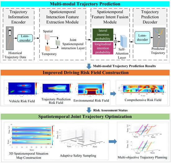
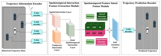
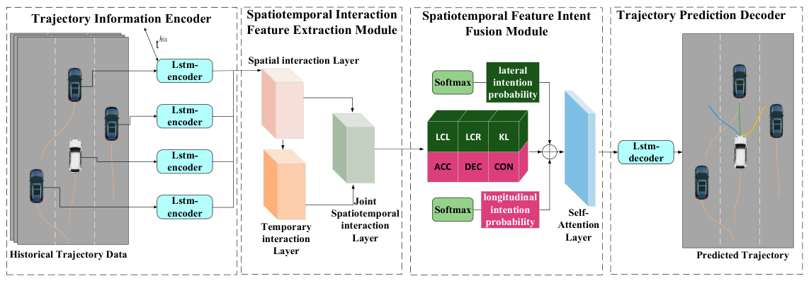
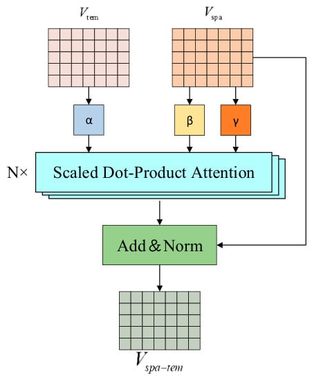
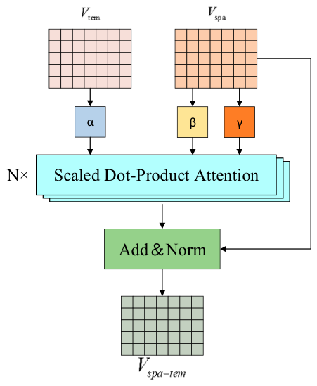
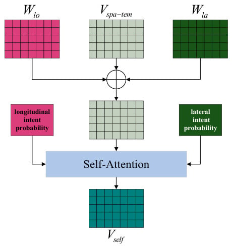
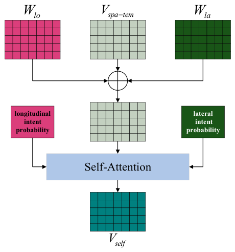
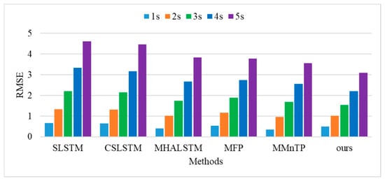
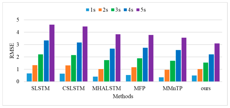
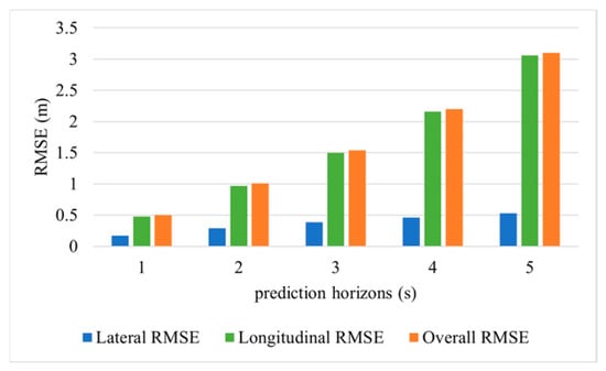
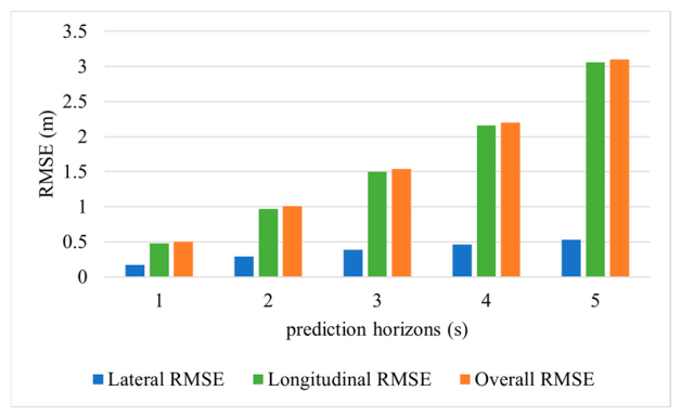
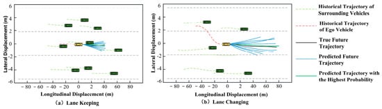
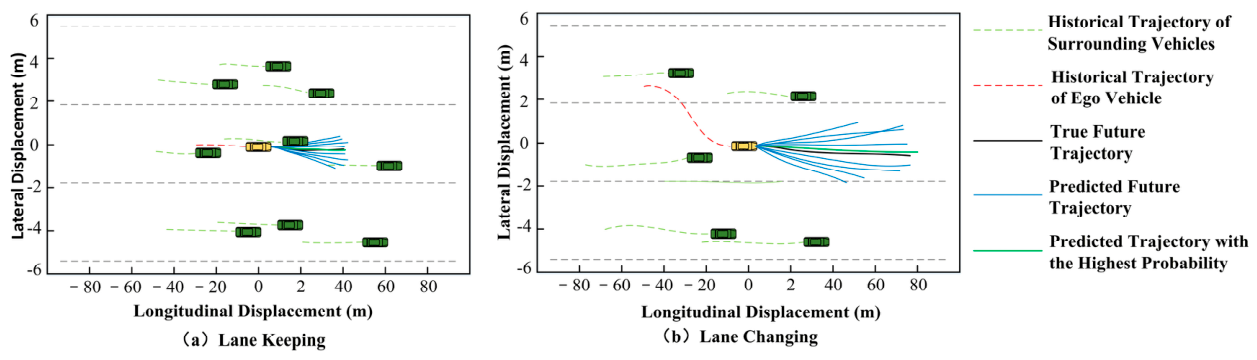


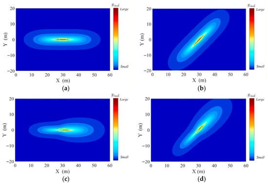
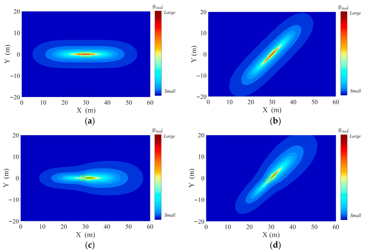
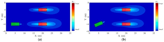
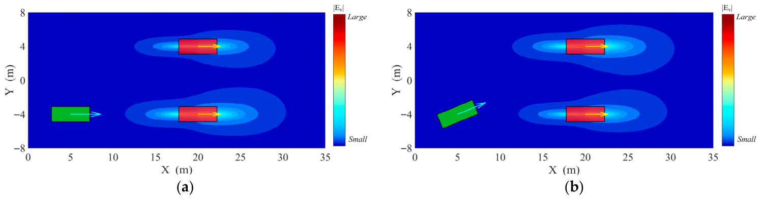
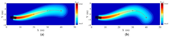
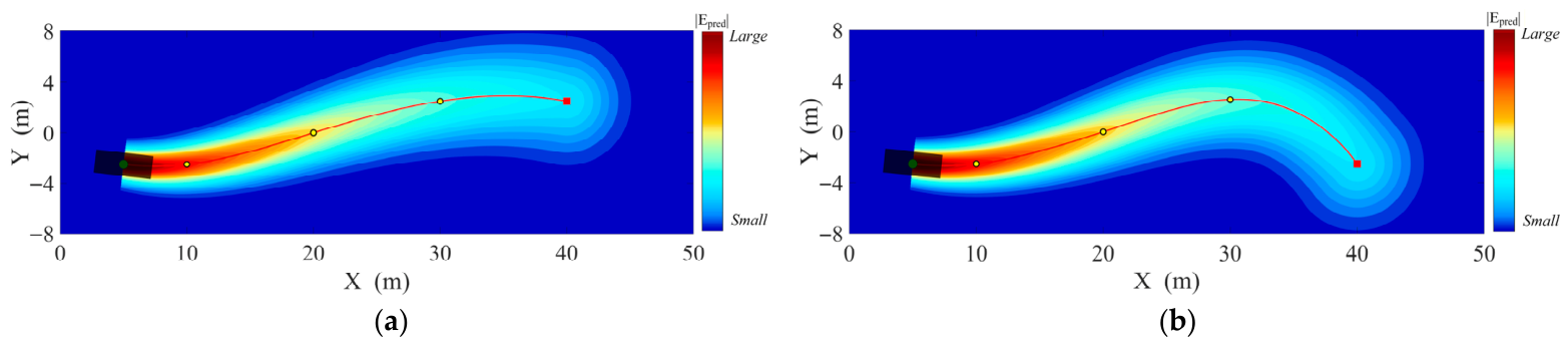
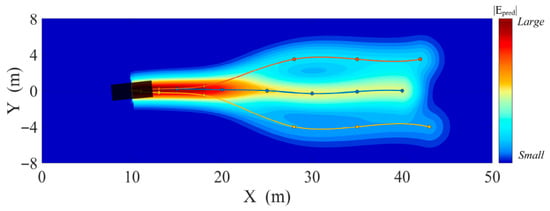
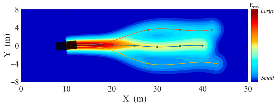
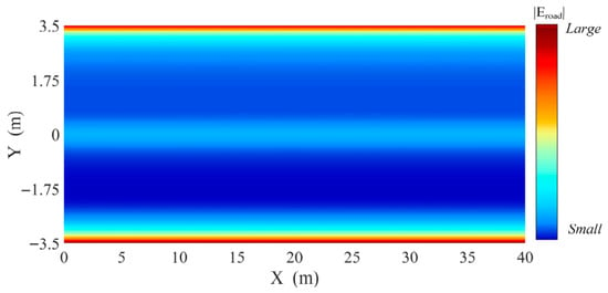
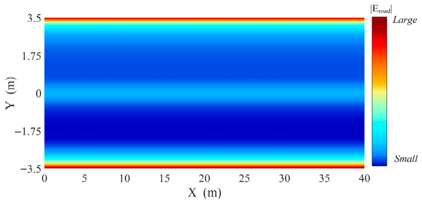
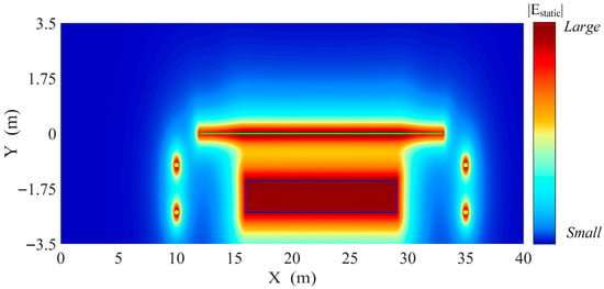
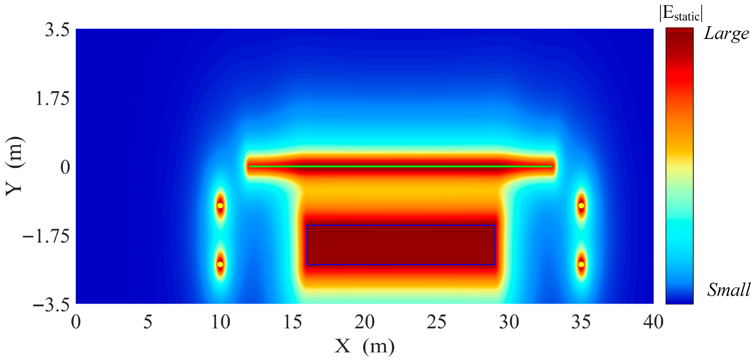
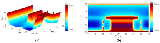
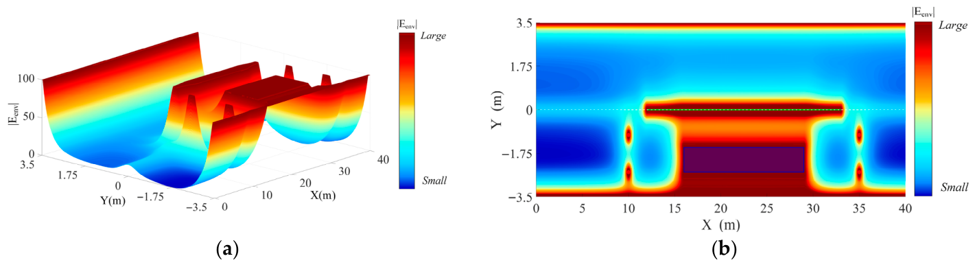
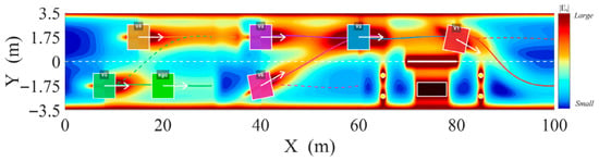
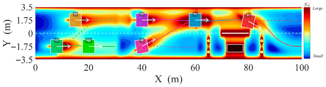
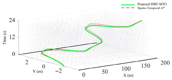
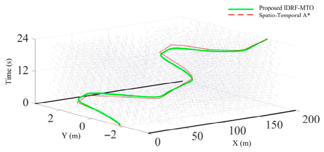
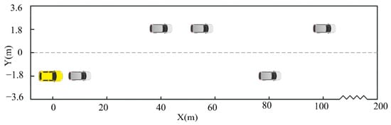
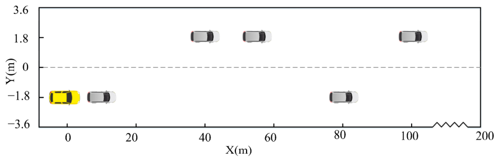
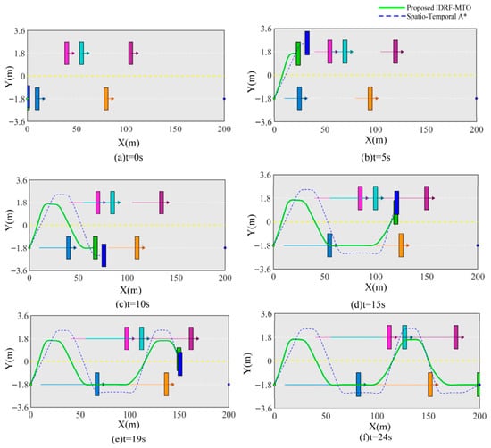
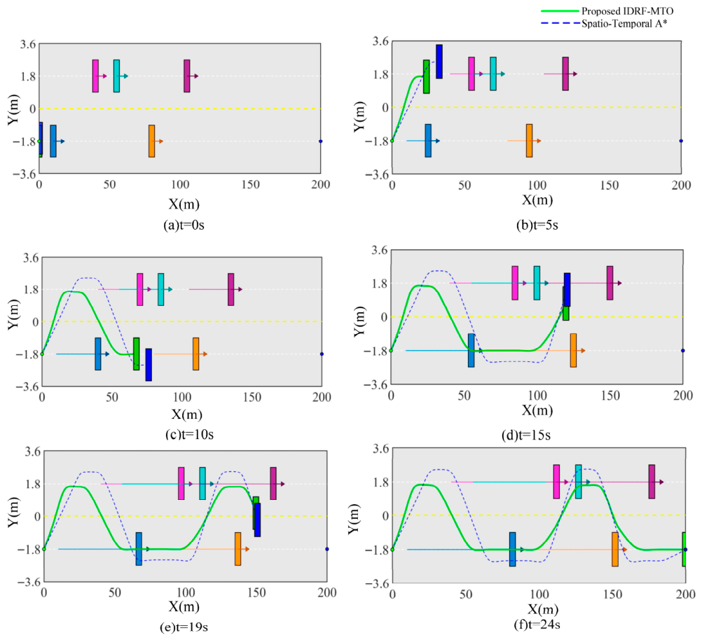
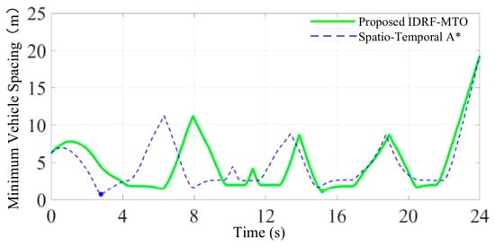
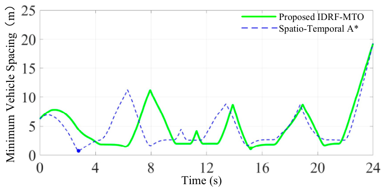
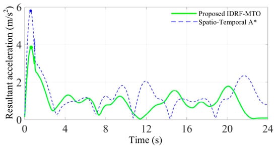
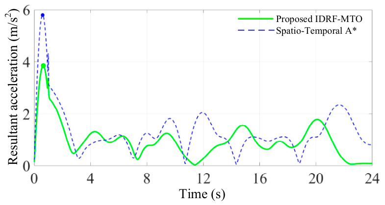
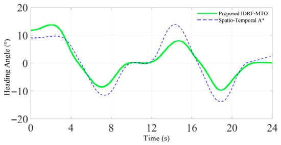
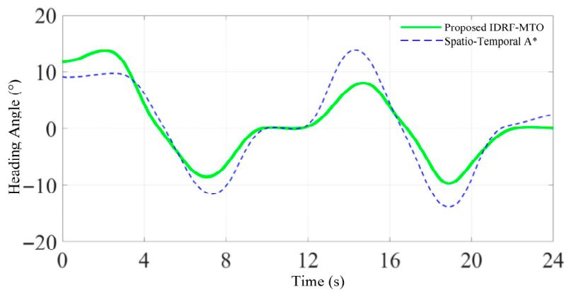
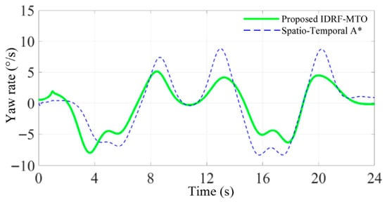
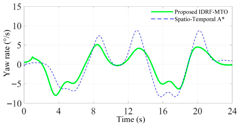
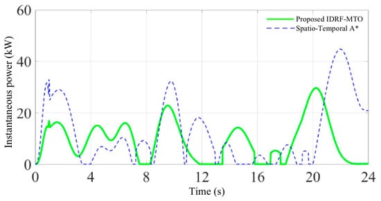
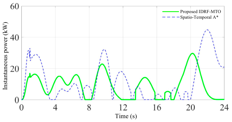
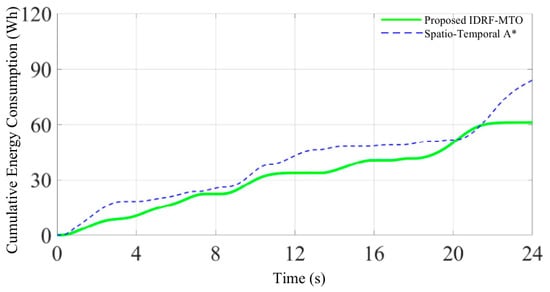
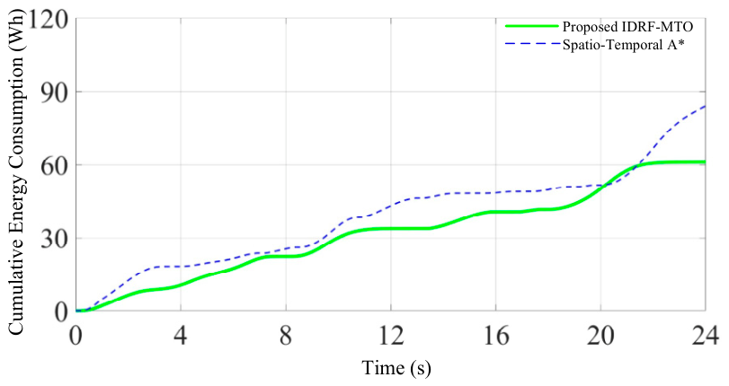

Disclaimer/Publisher’s Note: The statements, opinions and data contained in all publications are solely those of the individual author(s) and contributor(s) and not of MDPI and/or the editor(s). MDPI and/or the editor(s) disclaim responsibility for any injury to people or property resulting from any ideas, methods, instructions or products referred to in the content. |
© 2026 by the authors. Licensee MDPI, Basel, Switzerland. This article is an open access article distributed under the terms and conditions of the Creative Commons Attribution (CC BY) license.