Operation Prediction of a Gasification-Based Waste Treatment Plant Using Deep Learning

Abstract

In gasification-based waste treatment plants, continuous generation of combustible gas is essential for stable and efficient operation. To achieve this, multiple gasification furnaces are operated alternately; however, the internal states of the furnaces cannot be directly observed, making it difficult to assess the progress of gasification. Consequently, operation planning relies heavily on the experience of skilled operators. In this study, nonlinear system identification models based on deep learning are developed to predict the valve opening that controls the injection of gasification agents, which implicitly reflects the gasification state. Several modeling approaches, including linear finite impulse response (FIR) models, block-oriented Hammerstein–Wiener (HW) models, deep Hammerstein–Wiener models, and Transformer-based models, are investigated and compared. The models are trained and validated using actual operational data obtained from an industrial waste treatment plant. The results demonstrate that nonlinear models significantly outperform linear models, particularly for long-term prediction horizons. Among the examined approaches, the Transformer-based model shows stable and competitive performance across different prediction intervals. These findings indicate that deep learning-based nonlinear modeling is effective for predicting plant operation and has the potential to support automated operation planning, thereby reducing reliance on operator expertise.

1. Introduction

In recent years, artificial intelligence (AI) techniques have increasingly been applied to industrial plants, including waste treatment facilities, to improve operational efficiency and stability. Data-driven modeling has therefore attracted considerable attention in the field of process operation and monitoring [1,2,3,4]. In particular, gasification-based waste treatment plants, in which solid waste is gasified and the generated combustible gas is subsequently burned, have attracted significant attention [5]. Classical approaches such as autoregressive moving average (ARMA) models and FIR models have been widely used for modeling industrial processes [6,7]. Previous studies have applied machine learning techniques to tasks such as anomaly detection, short-term steam flow prediction, and estimation of gas composition in gasification processes [1,8].

For nonlinear dynamic systems, various system identification frameworks have been proposed [9,10,11]. Despite these advances, operation planning in gasification plants remains challenging. Because the internal state of a gasification furnace cannot be directly observed, it is difficult to assess the progress of gasification of the input waste [2,8]. As a result, operators must rely heavily on empirical knowledge to determine appropriate switching operations among multiple furnaces, which limits the potential for automation.

In this study, we focus on predicting the valve opening that controls the injection of gasification agents into the furnace. The valve opening is automatically adjusted to maintain the temperature of the combustion furnace within a desired range and therefore implicitly reflects the amount of combustible gas being generated. Unlike previous studies that directly predict physical quantities such as gas flow rates or gas compositions [3,10], this work targets the control variable itself, providing a more direct and operation-oriented indicator of the gasification state.

To address this problem, nonlinear system identification methods based on deep learning are investigated. Multiple model structures, including block-oriented models and Transformer-based architectures, are developed and compared using actual operational data obtained from an industrial waste treatment plant. The objective of this study is to clarify the effectiveness of nonlinear modeling approaches for long-term (multi-horizon) prediction of plant operation and to identify model structures suitable for practical deployment in industrial settings.

Unlike conventional soft sensor modeling approaches that focus on physical variables, this study addresses the prediction of a control-related variable that implicitly reflects the internal process state, providing an operation-oriented formulation that is more directly relevant to plant operation planning. In contrast to conventional control-oriented prediction tasks that focus on short-term or one-step-ahead forecasting, this study explicitly addresses multi-step prediction for operational planning purposes.

In summary, the main contributions of this study are as follows:

1.

This study presents, to the best of our knowledge, the first formulation of multi-horizon prediction of valve opening for gasification–incineration plant operation using real industrial data. While many previous studies have focused on physical variables such as gas composition and primarily addressed one-step-ahead prediction problems [12,13,14,15], the present study explicitly addresses multi-horizon prediction for operational planning.

2.

Unlike conventional soft sensor approaches that focus on physical variables, this study targets a control-related variable that implicitly reflects the internal process state, thereby providing an operation-oriented prediction framework.

3.

Multiple modeling approaches, including linear models, block-oriented models, and attention-based models, are systematically compared under a unified experimental setting, providing a benchmark for this application. Although comparative studies between machine learning and system identification methods have been reported in general process systems engineering [16], such a systematic comparison has not been conducted for gasification-based waste treatment processes.

4.

The proposed formulation is directly motivated by practical operational requirements, and the prediction results can be used as a decision-support tool for operational planning, such as waste feeding and resource allocation.

While the development of more advanced models, such as physics-informed or control-integrated approaches, is an important direction, this study focuses on establishing the fundamental problem formulation and benchmark for this class of industrial prediction tasks.

2. Operation Process of the Waste Treatment Plant

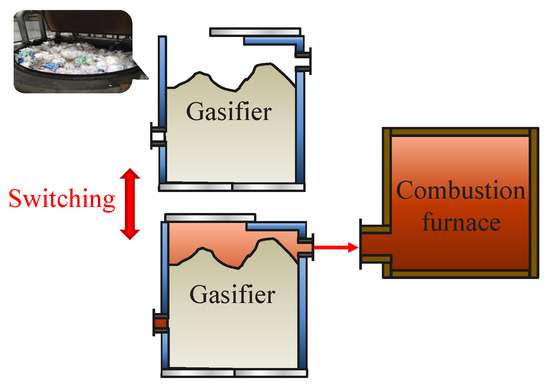
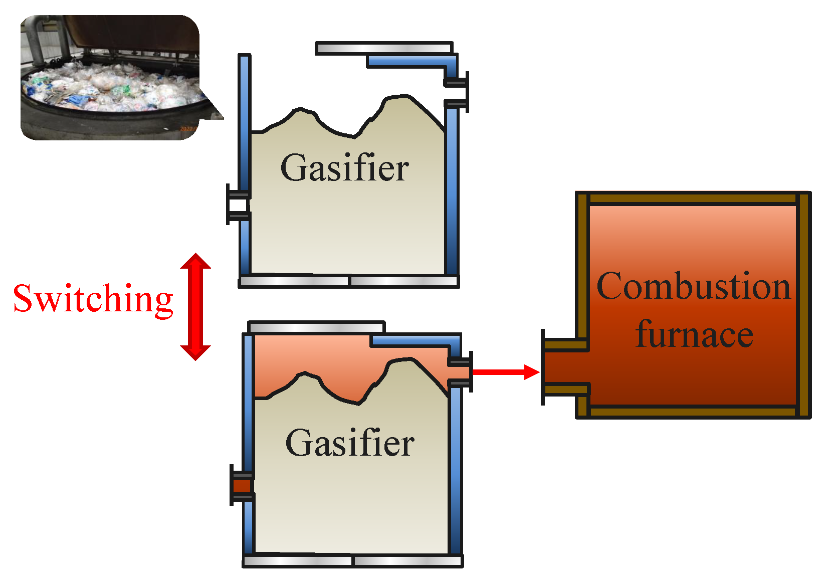
In this study, a waste treatment plant based on a gasification–incineration system is considered, in which waste is decomposed into combustible gas in a gasification furnace, and the generated gas is subsequently burned in a combustion furnace. Since the gasification process requires the furnace to be sealed and operated at high temperatures under oxygen-deficient conditions, waste charging and gasification cannot be performed simultaneously. Therefore, waste is charged into the gasification furnace in batches.

Combustion of the generated gas should be carried out within a temperature range that suppresses the formation of harmful substances. Therefore, in actual plant operation, a continuous gas supply is required to maintain a stable combustion furnace temperature. For this reason, as illustrated in Figure 1, multiple gasification furnaces are used, and the operation is alternated between furnaces for waste charging and for gasification, enabling continuous gas generation.

Figure 1. Process flow of the gasification-based waste treatment plant during operation.

In operation using multiple gasification furnaces, an ideal switching strategy requires that the preparation of the next furnace be completed before gas generation from the currently operating furnace ceases. However, several challenges arise in achieving this objective. One issue is that the internal state of the gasification furnace cannot be directly observed, making it impossible to directly determine the extent to which the charged waste has been gasified. Another issue is that several tons of waste are charged into the furnace at once. As a result, engineers determine the type of waste to be charged based on characteristics such as combustibility, and this process requires several hours. Due to these factors, achieving optimal operation timing requires estimating the gasification state from the present time to several hours ahead, so that subsequent operation can be appropriately planned.

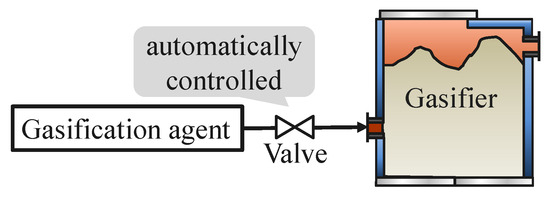
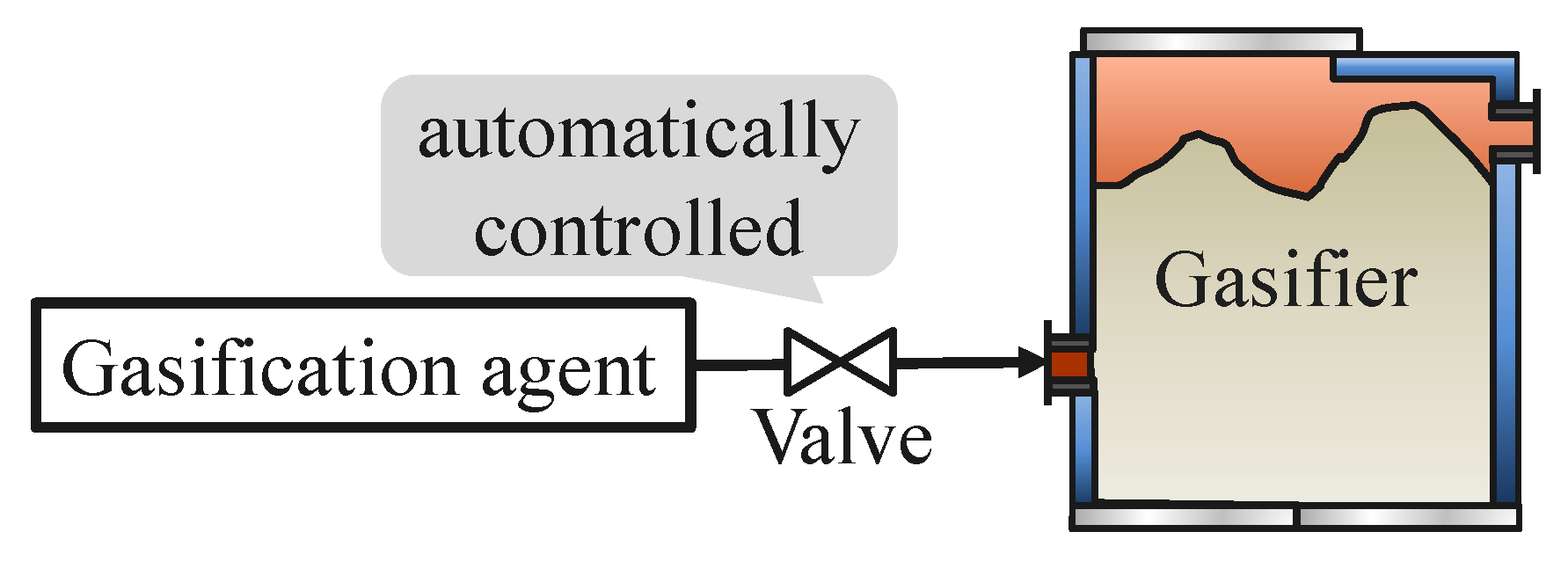
In this study, the valve opening that controls the injection of gasifying agents into the gasification furnace is used to characterize the gasification behavior, as shown in Figure 2, where a gasifying agent refers to a gas that assists the gasification process. The valve opening is automatically controlled to maintain the temperature of the combustion furnace at a constant level.

Figure 2. Relationship between the gasifier and the gasification agent supplied through an automatically controlled valve.

Under the automatic feedback control scheme, the valve opening is determined based on the balance between the gas generation rate in the gasification furnace and the thermal demand of the combustion furnace. When the gas generation rate increases, the combustion temperature rises, and the controller reduces the valve opening to suppress further gasification. Conversely, when the gas generation rate decreases, the valve opening is increased to promote gasification.

Therefore, although the valve opening is a control input rather than a direct measurement of the gasification process, it can be interpreted as an indirect indicator of the internal gasification state through the closed-loop control mechanism. In practical plant operation, operators also monitor the valve opening as an important indicator for decision-making.

The gasification state itself is not directly observable from the available data. Accordingly, the model considered in this study aims to capture the dynamics of the overall closed-loop system, which includes both the gasification process and the feedback control mechanism, rather than the intrinsic gasification process alone.

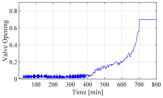
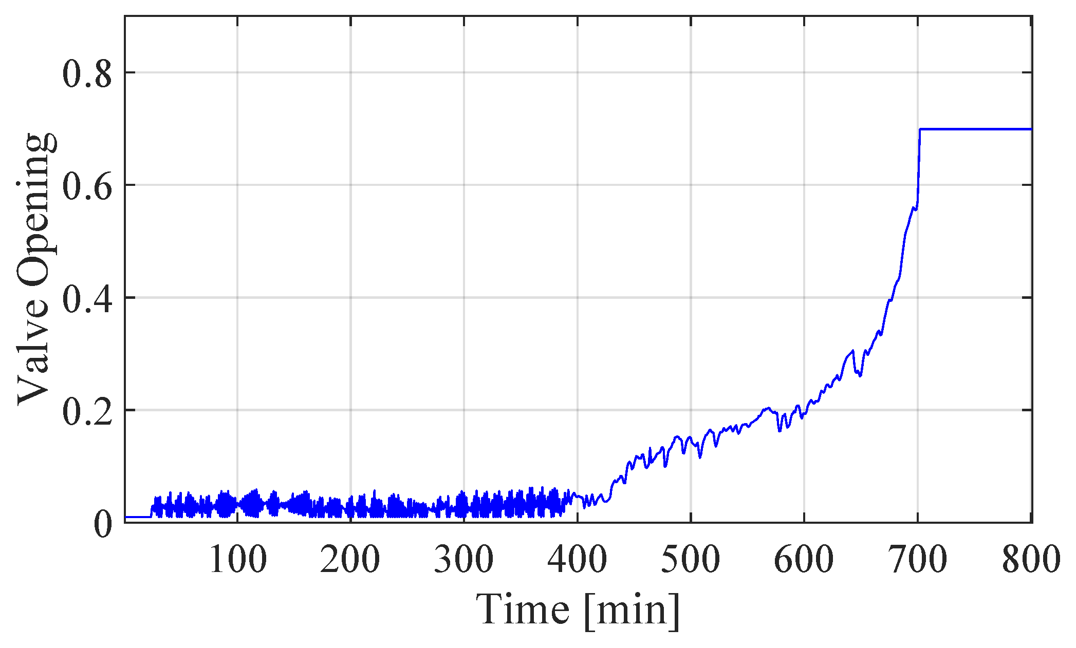
An example of the temporal variation in valve opening is shown in Figure 3. As shown in the figure, the valve opening increases over time and eventually levels off. Although there are slight variations depending on the specific plant, in this plant, the valve opening reaches approximately 0.7 and then stabilizes, as seen in Figure 3. Therefore, gasification is considered complete at this point.

Figure 3. Time-series transition of the valve opening during the gasification process in the waste treatment plant.

Based on the above operational background, this study aims to predict the progress of gasification by constructing a model that predicts the valve opening from the current time up to several hours ahead. In the following section, the modeling methods used to achieve this objective are described in detail.

3. Methodology

3.1. Problem Formulation

The operational data obtained from the plant include multiple physical quantities, such as the oxygen concentration and temperature of the combustion furnace and the temperature of the gasification furnace. Let these multivariate measurements be denoted by ${\mathbf{x}}_k\in {\mathbb{R}}^n$. In addition, let $y_k\in \mathbb{R}$ denote the valve opening to be predicted in this study, where k denotes the discrete time index.

Using the measurements ${\mathbf{x}}_k$, the objective is to predict the future valve openings at multiple prediction horizons. This multi-step prediction problem can be formulated as finding a function f that satisfies

$$\left[\begin{array}{c}{y}_{k+l_1}\\ y_{k+l_2}\\ ⋮\\ y_{k+l_p}\end{array}\right]=f\left({\mathbf{x}}_{k-o:h:k}, y_{k-o:h:k}\right),$$

(1)

where $l_1,\dots ,l_p$ represent the prediction horizons, o denotes the length of the past data used for prediction, and h represents the sampling interval of the input sequence. For a signal ${\xi }_k$, the notation ${\xi }_{a:h:b}$ denotes a sequence of values sampled at an interval of h from time a to time b, that is,

$${\xi }_{a:h:b}=\left\{{\xi }_k\mid k=a+\kappa h, 0\le \kappa \le {\displaystyle \frac{b-a}{h}}\right\},$$

(2)

where $\kappa$ is an integer index. When $h=1$, the notation is simplified and written as ${\xi }_{a:b}$.

In the following subsections, the model structures and implementation details required for constructing the function f in (1) are presented.

3.2. Hammerstein–Wiener Model

3.2.1. Block-Oriented Modeling Framework

In this study, block-oriented models are considered as a class of nonlinear system models that represent nonlinear dynamics by interconnecting linear dynamic elements and nonlinear static elements. Among various block-oriented structures, the HW model [9,10] is employed due to its flexibility and interpretability in modeling nonlinear dynamic systems. The HW model structure considered in this study is illustrated in Figure 4.

Figure 4. Structure of the Hammerstein–Wiener model, which represents a nonlinear system using nonlinear static blocks and a linear dynamic block.

The HW model consists of nonlinear static blocks placed before and after a linear dynamic block, enabling the representation of both nonlinear input–output relationships and temporal dynamics. This structure is particularly suitable for modeling plant operation data, where nonlinear effects and dynamic behavior are strongly coupled.

3.2.2. Linear Dynamic Element: Finite Impulse Response Model

The FIR model is employed as the linear dynamic element in the block-oriented structure. For a single-input single-output system, the FIR model is expressed as follows:

$${\widehat{y}}_k=\sum _{i=0}^m{g}_i{u}_{k-i},$$

(3)

where $u_k$ denotes the input to the model, ${\widehat{y}}_k$ represents the output of the model, $g_i$ denotes the impulse response coefficients, and m represents the model order.

For the multivariate case considered in this study, the FIR model is extended to

$${\widehat{\mathbf{y}}}_k={\mathbf{G}}_0{\mathbf{u}}_k+{\mathbf{G}}_1{\mathbf{u}}_{k-1}+\dots +{\mathbf{G}}_m{\mathbf{u}}_{k-m},$$

(4)

where ${\mathbf{u}}_k$ denotes the input vector, ${\widehat{\mathbf{y}}}_k$ represents the output vector, and ${\mathbf{G}}_i$ are the corresponding coefficient matrices.

This formulation represents a temporal convolution of the input sequence with FIR coefficients in the discrete-time domain. From this perspective, the FIR model can be interpreted as a special case of a temporal convolutional network (TCN) [17], where a fixed linear kernel is used and no nonlinear activation is applied. In this sense, the FIR model serves as a linear baseline for evaluating the effectiveness of nonlinear modeling approaches.

To unify the notation with subsequent nonlinear models, the multivariate FIR model in (4) is expressed as follows:

$$\mathrm{TCN}({\mathbf{u}}_{k-m:k}\mid \mathcal{G}):={\mathbf{G}}_0{\mathbf{u}}_k+{\mathbf{G}}_1{\mathbf{u}}_{k-1}+\dots +{\mathbf{G}}_m{\mathbf{u}}_{k-m},$$

(5)

where $\mathcal{G}=\{{\mathbf{G}}_0,\dots ,{\mathbf{G}}_m\}$ denotes the set of FIR coefficient matrices.

3.2.3. Nonlinear Static Element: Three-Layer Neural Network

The fully connected layer $\mathrm{FC}(·\mid ·,·)$ is defined as follows:

$$\mathrm{FC}(\mathbf{x}\mid \mathbf{W},\mathbf{b}):=\mathbf{W}\mathbf{x}+\mathbf{b},$$

(6)

where $\mathbf{W}$ and $\mathbf{b}$ denote the weight matrix and bias vector, respectively. The rectified linear unit (ReLU) activation function is given by

$$\mathrm{ReLU}\left(\mathbf{x}\right)=max(\mathbf{x},0),$$

(7)

where the maximum operation is applied element-wise.

In this study, a three-layer neural network (NN) is employed as the nonlinear static element in the HW model. The neural network is defined as follows:

$$\mathrm{NN}(\mathbf{x}\mid \mathcal{P}):=\mathrm{FC}\left(\mathrm{ReLU}\left(\mathrm{FC}(\mathbf{x}\mid {\mathbf{W}}_1,{\mathbf{b}}_1)\right) | {\mathbf{W}}_2,{\mathbf{b}}_2\right),$$

(8)

where $\mathbf{x}$ denotes the input feature vector to the neural network, and ${\mathbf{W}}_1,{\mathbf{W}}_2$ and ${\mathbf{b}}_1,{\mathbf{b}}_2$ are the weight matrices and bias vectors, respectively. The set of trainable parameters is defined as follows:

$$\mathcal{P}=\{{\mathbf{W}}_1,{\mathbf{b}}_1,{\mathbf{W}}_2,{\mathbf{b}}_2\}.$$

(9)

3.3. Deep Hammerstein–Wiener Model

When the FIR-based TCN and the three-layer neural network are employed as the linear dynamic and nonlinear static elements, respectively, a HW model is constructed. The model structure shown in Figure 4 is expressed as follows:

$$\begin{array}{cc}\hfill {\widehat{\mathbf{y}}}_k & =\mathrm{NN}\left({\mathbf{z}}_k^{\left(1\right)}\mid {\mathcal{P}}^{\left(1\right)}\right),\hfill \end{array}$$

(10)

$$\begin{array}{cc}\hfill {\mathbf{z}}_k^{\left(1\right)} & =\mathrm{TCN}\left({\mathbf{z}}_{k-m:k}^{\left(2\right)}\mid {\mathcal{G}}^{\left(2\right)}\right),\hfill \end{array}$$

(11)

$$\begin{array}{cc}\hfill {\mathbf{z}}_k^{\left(2\right)} & =\mathrm{NN}\left({\mathbf{u}}_k\mid {\mathcal{P}}^{\left(3\right)}\right).\hfill \end{array}$$

(12)

where ${\widehat{\mathbf{y}}}_k$ denotes the predicted output vector at time step k, ${\mathbf{u}}_k$ denotes the input vector, ${\mathbf{z}}_k^{\left(i\right)}$ represents the intermediate signal at the i-th layer of the HW model, and ${\mathcal{P}}^{\left(i\right)}$ and ${\mathcal{G}}^{\left(i\right)}$ denote the parameter sets of the i-th layer. Furthermore, a deep HW model can be constructed by stacking multiple nonlinear static and linear dynamic elements. The deep HW model is formulated as follows:

$$\begin{array}{cc}\hfill {\widehat{\mathbf{y}}}_k & =\mathrm{NN}\left({\mathbf{z}}_k^{\left(1\right)}\mid {\mathcal{P}}^{\left(1\right)}\right),\hfill \end{array}$$

(13)

$$\begin{array}{cc}\hfill {\mathbf{z}}_k^{\left(1\right)} & =\mathrm{TCN}\left({\mathbf{z}}_{k-n:k}^{\left(2\right)}\mid {\mathcal{G}}^{\left(2\right)}\right),\hfill \end{array}$$

(14)

$$\begin{array}{cc}\hfill {\mathbf{z}}_k^{\left(2\right)} & =\mathrm{NN}\left({\mathbf{z}}_k^{\left(3\right)}\mid {\mathcal{P}}^{\left(3\right)}\right),\hfill \\ \hfill & ⋮\hfill \end{array}$$

(15)

$$\begin{array}{cc}\hfill {\mathbf{z}}_k^{(M-2)} & =\mathrm{TCN}\left({\mathbf{z}}_{k-n:k}^{(M-1)}\mid {\mathcal{G}}^{(M-1)}\right),\hfill \end{array}$$

(16)

$$\begin{array}{cc}\hfill {\mathbf{z}}_k^{(M-1)} & =\mathrm{NN}\left({\mathbf{u}}_k\mid {\mathcal{P}}^{\left(M\right)}\right),\hfill \end{array}$$

(17)

where M denotes the number of stacked layers in the deep HW model.

Since both $\mathrm{NN}$ and $\mathrm{TCN}$ are neural network-based models, the entire HW structure can be interpreted as a single deep neural network. Accordingly, all model parameters can be efficiently trained using modern deep learning frameworks, such as PyTorch 2.10.0 or the Deep Learning Toolbox in MATLAB R2024b [18].

3.4. Transformer

Transformer models, originally proposed for natural language processing [19], have recently been extended to time-series prediction tasks through attention-based architectures, including recurrent attention-based models [20] and Transformer variants specialized for long-term forecasting [21,22,23]. In this subsection, the model structures required for implementation are described.

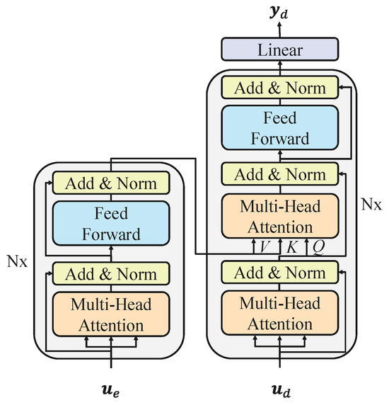
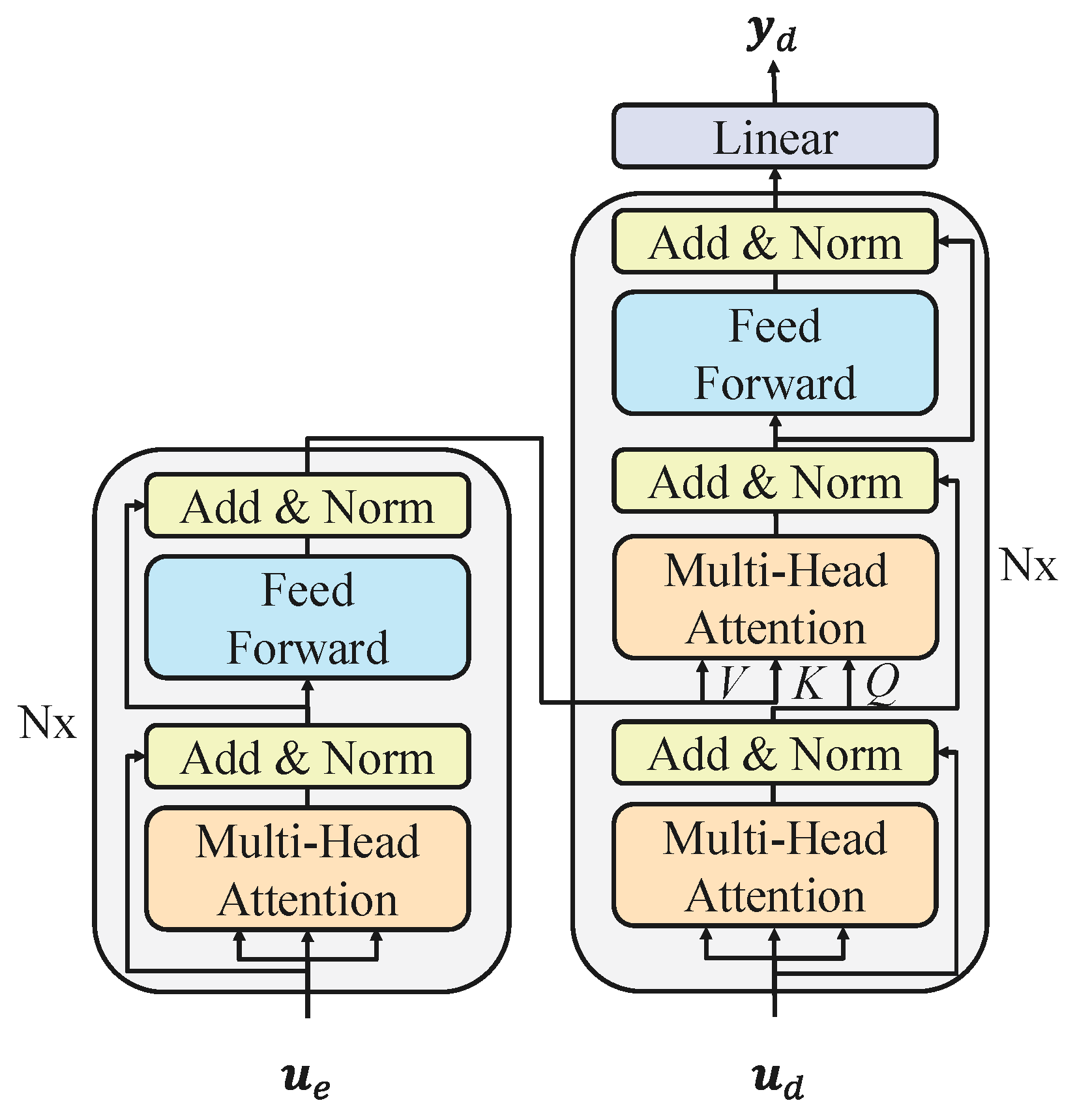
Figure 5 illustrates the overall structure of the Transformer-based model used in this study.

Figure 5. Architecture of the transformer-based prediction model.

The Transformer adopts an encoder–decoder architecture, which is widely used for sequence transformation tasks. Both the encoder and the decoder consist of attention mechanisms and feed-forward networks, and each component is connected via residual connections. Furthermore, the encoder and the decoder are each composed of N stacked layers.

The entire Transformer model used in this study is expressed as follows:

$${\mathbf{Y}}_d=\mathrm{Transformer}\left({\mathbf{U}}_e,{\mathbf{U}}_d\right),$$

(18)

where ${\mathbf{U}}_e\in {\mathbb{R}}^{n\times d_{\mathrm{model}}}$ is the input to the encoder, ${\mathbf{U}}_d\in {\mathbb{R}}^{m\times d_{\mathrm{model}}}$ is the input to the decoder, and ${\mathbf{Y}}_d\in {\mathbb{R}}^{m\times d_{\mathrm{output}}}$ is the output of the decoder. Here, n denotes the length of the encoder input sequence, m denotes the length of the decoder input and output sequences, and $d_{\mathrm{model}}$ and $d_{\mathrm{output}}$ represent the data dimensions. For time-series data, the temporal length corresponds to the encoder input sequence length n, while the feature dimension corresponds to $d_{\mathrm{model}}$.

3.4.1. Scaled Dot-Product Attention

The attention mechanism is a function with three inputs, namely Query ($\mathbf{Q}$), Key ($\mathbf{K}$), and Value ($\mathbf{V}$), and is defined as follows:

$$\mathrm{Attention}\left(\mathbf{Q},\mathbf{K},\mathbf{V}\right)=\mathrm{softmax}\left({\displaystyle \frac{\mathbf{Q}{\mathbf{K}}^{\top }}{\sqrt{d_k}}}\right)\mathbf{V}.$$

(19)

Here, $\mathbf{Q}\in {\mathbb{R}}^{p\times d_k}$, $\mathbf{K}\in {\mathbb{R}}^{q\times d_k}$, and $\mathbf{V}\in {\mathbb{R}}^{q\times d_v}$, where p and q denote the lengths of the query and key/value sequences, and $d_k$ and $d_v$ denote the dimensions of the key/query vectors and the value vectors, respectively. When $d_k$ is large, the gradients of the softmax function may become excessively small. To mitigate this issue, the dot product of $\mathbf{Q}$ and $\mathbf{K}$ is scaled by $\sqrt{d_k}$. This mechanism is referred to as scaled dot-product attention.

3.4.2. Multi-Head Attention

Instead of performing a single attention operation, multiple attention operations are computed in parallel. This mechanism is called multi-head attention and is defined as follows:

$$\mathrm{MultiHead}\left(\mathbf{Q},\mathbf{K},\mathbf{V}\right)=\mathrm{Concat}\left({\mathrm{head}}_1,\dots ,{\mathrm{head}}_h\right){\mathbf{W}}_O,$$

(20)

where h denotes the number of attention heads and $\mathrm{Concat}(·)$ represents the concatenation operation. Each head is given by

$${\mathrm{head}}_i=\mathrm{Attention}\left({\mathbf{QW}}_i^Q,{\mathbf{KW}}_i^K,{\mathbf{VW}}_i^V\right),$$

(21)

where ${\mathbf{W}}_i^Q\in {\mathbb{R}}^{d_{\mathrm{model}}\times d_k}$, ${\mathbf{W}}_i^K\in {\mathbb{R}}^{d_{\mathrm{model}}\times d_k}$, ${\mathbf{W}}_i^V\in {\mathbb{R}}^{d_{\mathrm{model}}\times d_v}$, and ${\mathbf{W}}_O\in {\mathbb{R}}^{h{d}_k\times d_{\mathrm{model}}}$. Multi-head attention enables the model to attend to information at different temporal positions simultaneously by projecting the inputs into multiple representation subspaces.

3.4.3. Position-Wise Feed-Forward Network

In addition to the attention mechanism, both the encoder and decoder include a feed-forward network (FFN) defined as follows:

$$\mathrm{FFN}(\mathbf{x}\mid \mathcal{P})=\mathrm{FC}\left(\mathrm{ReLU}\left(\mathrm{FC}(\mathbf{x}\mid {\mathbf{W}}_1,{\mathbf{b}}_1)\right) | {\mathbf{W}}_2,{\mathbf{b}}_2\right),$$

(22)

where $\mathrm{FC}(·)$ denotes a fully connected linear transformation and $\mathcal{P}=\{{\mathbf{W}}_1,{\mathbf{b}}_1,{\mathbf{W}}_2,{\mathbf{b}}_2\}$ denotes the parameter set of the FFN. The weight matrices satisfy ${\mathbf{W}}_1\in {\mathbb{R}}^{d_{\mathrm{model}}\times d_{\mathrm{ff}}}$ and ${\mathbf{W}}_2\in {\mathbb{R}}^{d_{\mathrm{ff}}\times d_{\mathrm{model}}}$. This operation is applied independently and identically to each position in the input sequence. The input and output dimensions are $d_{\mathrm{model}}$, while the internal dimension is denoted by $d_{\mathrm{ff}}$.

3.4.4. Residual Connection and Layer Normalization

In the Transformer architecture, residual connections and layer normalization are applied to each sublayer. This process is referred to as Add & Norm. The operation is expressed as follows:

$$\mathbf{y}=\mathrm{LayerNorm}\left(\mathbf{x}+\mathrm{Sublayer}\left(\mathbf{x}\right)\right),$$

(23)

where $\mathrm{Sublayer}\left(\mathbf{x}\right)$ denotes the output of the layer immediately preceding Add & Norm.

Residual connections facilitate optimization and enable performance improvements as the network depth increases [24]. Layer normalization is defined as follows:

$$\mathrm{LayerNorm}\left(x_i^{\left(l\right)}\right)={\gamma }_l{\displaystyle \frac{x_i^{\left(l\right)}-{\mu }_l}{{\sigma }_l}}+{\beta }_l,$$

(24)

with

$$\begin{array}{cc}\hfill {\mu }_l & ={\displaystyle \frac{1}{H}}\sum _{i=1}^H{x}_i^{\left(l\right)},\hfill \end{array}$$

(25)

$$\begin{array}{cc}\hfill {\sigma }_l & =\sqrt{{\displaystyle \frac{1}{H}}\sum _{i=1}^H{\left(x_i^{\left(l\right)}-{\mu }_l\right)}^2},\hfill \end{array}$$

(26)

where $x_i^{\left(l\right)}$ denotes the i-th element of the input vector ${\mathbf{x}}^{\left(l\right)}\in {\mathbb{R}}^H$ to the layer normalization, ${\mu }_l$ and ${\sigma }_l$ denote the mean and standard deviation of ${\mathbf{x}}^{\left(l\right)}$, and ${\gamma }_l$ and ${\beta }_l$ are learnable scaling and bias parameters. Layer normalization stabilizes gradients within the network and has been shown to reduce training time [25].

3.4.5. Output Layer

In the Transformer architecture, the input dimensions of the encoder and decoder, $d_{\mathrm{model}}$, must be identical, and the output of the decoder also has dimension $d_{\mathrm{model}}$. In this study, to allow the output dimension to be determined arbitrarily according to the prediction task, a linear output layer is added as follows:

$${\mathbf{Y}}_d={\mathbf{Y}}_d^{\prime }{\mathbf{W}}_o,$$

(27)

where ${\mathbf{Y}}_d^{\prime }\in {\mathbb{R}}^{m\times d_{\mathrm{model}}}$ denotes the decoder output before the linear layer, ${\mathbf{Y}}_d\in {\mathbb{R}}^{m\times d_{\mathrm{output}}}$ is the final model output, m denotes the decoder sequence length, and ${\mathbf{W}}_o\in {\mathbb{R}}^{d_{\mathrm{model}}\times d_{\mathrm{output}}}$ is a learnable weight matrix of the linear projection.

3.5. Comparison Between Hammerstein–Wiener and Transformer Models

The HW and Transformer models are based on distinct modeling philosophies for nonlinear time-series prediction. The HW model explicitly represents a system as a cascade of nonlinear static elements and linear dynamic elements, thereby enabling a structured modeling approach that can incorporate prior knowledge of system dynamics. This block-oriented formulation enhances interpretability and allows the temporal behavior of the system to be described in a physically meaningful manner.

In contrast, the Transformer model learns temporal dependencies in an end-to-end manner through attention mechanisms, without explicitly imposing a predefined dynamic structure. By exploiting self-attention, the Transformer can flexibly capture long-range temporal dependencies in time-series data, which is advantageous for long-horizon prediction tasks. While this approach provides high modeling flexibility and expressive power, the resulting model structure is generally less interpretable than that of block-oriented models.

By evaluating these two modeling approaches using the same operational dataset, this study aims to elucidate the trade-offs between structured nonlinear modeling and data-driven sequence modeling in the context of industrial plant operation prediction.

4. Prediction Modeling Using Actual Operational Data

In this section, the model structures described in the previous section are applied to the problem formulated in (1). Specifically, a prediction model is constructed using 24 measured variables obtained from the plant, including the valve opening. Five hours of past operational data are used to predict the valve openings at 30-min intervals from 30 min to 5 h ahead. The operational data are discrete time-series sampled at a period of 1 min.

Accordingly, the modeling problem considered in this study is to construct a function f that satisfies

$$\widehat{\mathbf{y}}=f\left({\chi }_{k-300:k}\right),$$

(28)

where the predicted valve openings are given by

$$\widehat{\mathbf{y}}={\left[{\widehat{y}}_{k+30},{\widehat{y}}_{k+60},\dots ,{\widehat{y}}_{k+300}\right]}^{\top },$$

(29)

and ${\chi }_k={[{\mathbf{x}}_k^{\top },y_k]}^{\top }$ denotes the operational data at time step k, where ${\mathbf{x}}_k\in {\mathbb{R}}^{23}$ represents the vector of plant variables other than the valve opening and $y_k$ denotes the valve opening.

4.1. Operational Dataset from the Gasification-Based Waste Treatment Plant

The dataset used in this study was obtained from an industrial gasification-based waste treatment plant. A total of 821 operational datasets is available. Among them, 738 datasets are used for training the models, while the remaining 83 datasets are reserved for validation. Although 738 operation datasets were used for training, each dataset was further divided into approximately 400–500 temporal slices for supervised learning. Therefore, the effective number of training samples was substantially larger than the number of operation datasets themselves. The training and validation datasets are separated on an operation-by-operation basis to avoid information leakage between datasets. Prior to model training, all input variables are normalized to improve training stability. The same normalization parameters are applied to both the training and validation datasets.

4.2. Prediction Model Configuration

In this subsection, the model structures described in Section 3 are instantiated for the valve opening prediction problem using actual operational data.

4.2.1. Finite Impulse Response Model

To discuss the necessity of nonlinear components in the valve opening prediction task, a prediction model based on a linear FIR model is constructed as a baseline. By applying (4) to the problem formulated in Section 3.2, the FIR-based prediction model is given by

$$\mathbf{y}={\mathbf{G}}_0{\chi }_k+{\mathbf{G}}_1{\chi }_{k-1}+\dots +{\mathbf{G}}_{300}{\chi }_{k-300},$$

(30)

where ${\chi }_k$ denotes the operational data, including the valve opening.

4.2.2. Hammerstein–Wiener Model

By applying the HW model described in Section 3.2 to the valve opening prediction problem, the model can be expressed as follows:

$$\begin{array}{cc}\hfill \widehat{\mathbf{y}} & =\mathrm{NN}\left({\mathbf{z}}_k^{\left(1\right)}\mid {\mathcal{P}}^{\left(1\right)}\right),\hfill \end{array}$$

(31)

$$\begin{array}{cc}\hfill {\mathbf{z}}_k^{\left(1\right)} & =\mathrm{TCN}\left({\mathbf{z}}_{k-300:k}^{\left(2\right)}\mid {\mathcal{G}}^{\left(2\right)}\right),\hfill \end{array}$$

(32)

$$\begin{array}{cc}\hfill {\mathbf{z}}_k^{\left(2\right)} & =\mathrm{NN}\left({\chi }_k\mid {\mathcal{P}}^{\left(3\right)}\right).\hfill \end{array}$$

(33)

4.2.3. Deep Hammerstein–Wiener Model

A deep HW model with $M=7$ layers is also considered following the framework described in Section 3.2. The model is formulated as follows:

$$\begin{array}{cc}\hfill {\widehat{\mathbf{y}}}_k & =\mathrm{NN}\left({\mathbf{z}}_k^{\left(1\right)}\mid {\mathcal{P}}^{\left(1\right)}\right),\hfill \end{array}$$

(34)

$$\begin{array}{cc}\hfill {\mathbf{z}}_k^{\left(1\right)} & =\mathrm{TCN}\left({\mathbf{z}}_{k-100:k}^{\left(2\right)}\mid {\mathcal{G}}^{\left(2\right)}\right),\hfill \end{array}$$

(35)

$$\begin{array}{cc}\hfill {\mathbf{z}}_k^{\left(2\right)} & =\mathrm{NN}\left({\mathbf{z}}_k^{\left(3\right)}\mid {\mathcal{P}}^{\left(3\right)}\right),\hfill \end{array}$$

(36)

$$\begin{array}{cc}\hfill {\mathbf{z}}_k^{\left(3\right)} & =\mathrm{TCN}\left({\mathbf{z}}_{k-100:k}^{\left(4\right)}\mid {\mathcal{G}}^{\left(4\right)}\right),\hfill \end{array}$$

(37)

$$\begin{array}{cc}\hfill {\mathbf{z}}_k^{\left(4\right)} & =\mathrm{NN}\left({\mathbf{z}}_k^{\left(5\right)}\mid {\mathcal{P}}^{\left(5\right)}\right),\hfill \end{array}$$

(38)

$$\begin{array}{cc}\hfill {\mathbf{z}}_k^{\left(5\right)} & =\mathrm{TCN}\left({\mathbf{z}}_{k-100:k}^{\left(6\right)}\mid {\mathcal{G}}^{\left(6\right)}\right),\hfill \end{array}$$

(39)

$$\begin{array}{cc}\hfill {\mathbf{z}}_k^{\left(6\right)} & =\mathrm{NN}\left({\chi }_k\mid {\mathcal{P}}^{\left(7\right)}\right).\hfill \end{array}$$

(40)

Note that the index ranges of ${\mathbf{z}}_k^{\left(2\right)}$, ${\mathbf{z}}_k^{\left(4\right)}$, and ${\mathbf{z}}_k^{\left(6\right)}$ are set to $k-100$:k instead of $k-300$:k. This configuration ensures that the total amount of past data used in the model corresponds to five hours (300 time steps). Specifically, in (37), the term ${\mathbf{z}}_{k-100}^{\left(4\right)}$ is used. As can be seen from (38) and (39), this term is computed from ${\mathbf{z}}_{k-200:k-100}^{\left(6\right)}$. This implies that the information in ${\chi }_{k-200:k}$ is effectively incorporated at this layer. By applying the same reasoning recursively to the preceding layers, it can be confirmed that the final prediction ${\widehat{\mathbf{y}}}_k$ utilizes the information contained in ${\chi }_{k-300:k}$.

4.2.4. Transformer-Based Model

As described in Section 3.4, when time-series data are applied to a Transformer model, the temporal length of the data corresponds to the number of rows in ${\mathbf{U}}_e$, while the feature dimension corresponds to the number of columns in ${\mathbf{U}}_e$ and ${\mathbf{U}}_d$. Although the encoder and decoder inputs may have different temporal lengths, their data dimensions must be identical. In addition, the temporal length of the decoder output corresponds to that of the decoder input.

Based on these conditions, a Transformer model that satisfies (1) is defined as follows:

$$\widehat{\mathbf{y}}=\mathrm{Transformer}\left({\chi }_{k-300:k},{\chi }_{k-300:30:k}\right).$$

(41)

In this configuration, the encoder receives raw operational data over the past five hours, while the decoder receives operational data sampled at 30-min intervals over the same period. By this design, the model predicts the valve openings at 30-min intervals for the next five hours.

4.3. Training Conditions and Hyperparameters

Each model includes several user-defined hyperparameters. In this study, the hyperparameters and the corresponding model sizes are summarized in Table 1 and Table 2, respectively. Table 2 provides the approximate numbers of trainable parameters for each model. In addition to the models described in Section 3, recurrent neural network-based models, namely the long short-term memory (LSTM) and gated recurrent unit (GRU) [26], are also included in Table 2 for reference, and their performance is evaluated in the subsequent section.

Table 1. Hyperparameter settings used for training the prediction models.

Hyperparameter	Value
Hidden nodes in three-layer NN ($d_h$)	128
Multi-head attention dimensions ($d_k$, $d_v$)	32
Number of attention heads (h)	4
Feed-forward network dimension ($d_{\mathrm{ff}}$)	128
Training epochs	100
Initial learning rate	$1\times {10}^{-5}$
Learning rate decay	$1\times {10}^{-8}$
Number of training datasets	738
Number of validation datasets	83

Table 2. Number of trainable parameters for each model.

Model	Number of Trainable Parameters
FIR model	∼$7.2\times {10}^4$
HW model	∼$3.7\times {10}^4$
Deep HW model	∼$4.3\times {10}^4$
LSTM model	∼$8.0\times {10}^4$
GRU model	∼$6.0\times {10}^4$
Transformer-based model	∼$7.6\times {10}^4$

The parameter $d_h$ denotes the number of hidden nodes in the hidden layer of the three-layer neural network used as the nonlinear static element in the block-oriented models. This parameter is shared by both the HW model and the deep HW model. In the Transformer model, $d_k$ and $d_v$ represent the dimensions used to project the input with dimension $d_{\mathrm{model}}=h\times d_k$ into the query, key, and value spaces, respectively. The parameter h denotes the number of parallel attention heads, and $d_{\mathrm{ff}}$ represents the dimension of the intermediate layer in the position-wise feed-forward network. The number of training epochs, the initial learning rate, and the learning rate decay are also listed in Table 1. For simplicity, all encoder layers share the same architecture and hyperparameter settings, and all decoder layers are configured in the same manner. The hyperparameters used in the Transformer model (i.e., $d_k=d_v=32$, $h=4$, and $d_{\mathrm{model}}=128$) are chosen to be consistent with commonly used configurations in Transformer-based models. In practice, these values were determined through preliminary trial-and-error experiments. A systematic hyperparameter tuning or sensitivity analysis has not been conducted in this study and is left as future work.

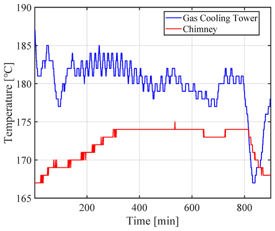
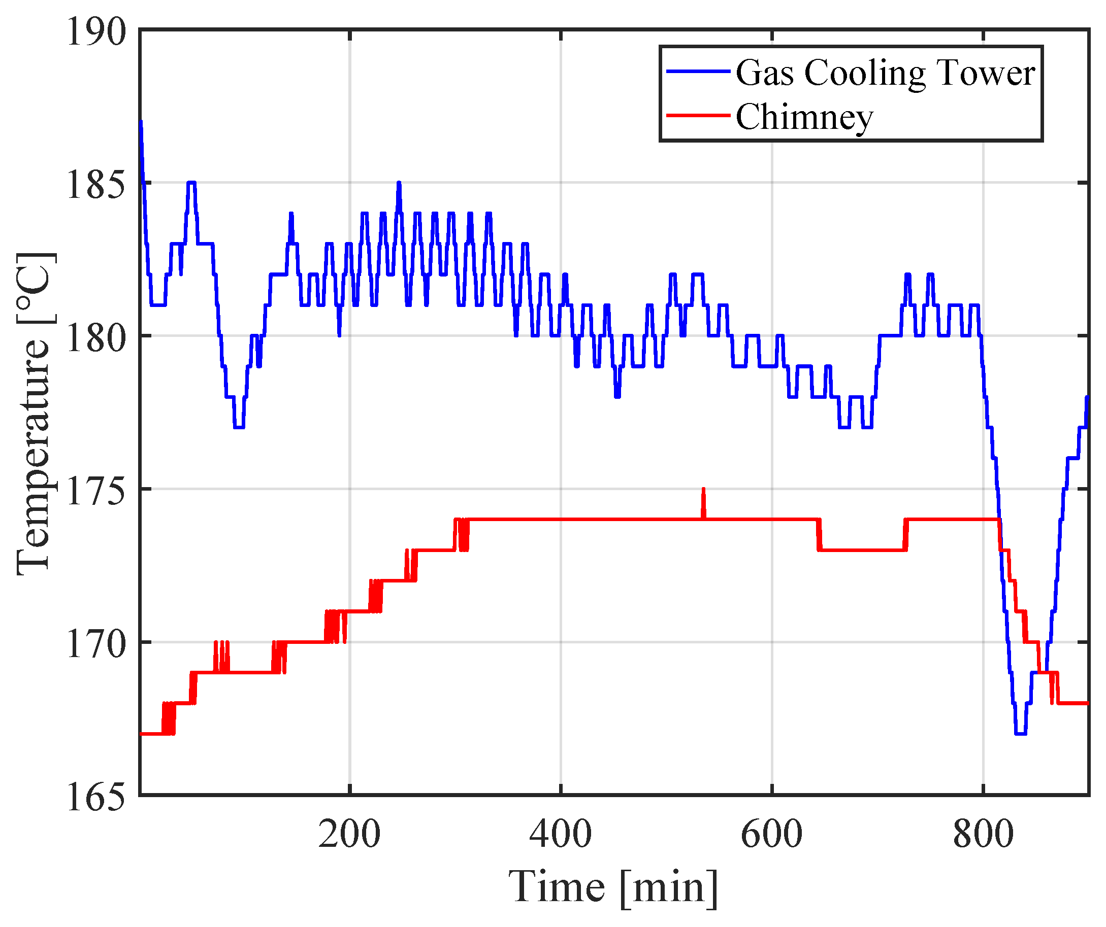
Figure 6 shows a subset of the operational data excluding the valve opening, specifically the temperatures of the quench tower used for exhaust gas cooling and the exhaust stack. These variables provide representative examples of the plant operating conditions used for model training and validation.

Figure 6. Example of operational data obtained from the waste treatment plant during plant operation.

4.4. Results

Table 3 summarizes the prediction performance of each model on both the training and validation datasets. In addition to the models described in Section 3, the LSTM and GRU models are also included as representative recurrent neural network-based baselines for comparison.

Table 3. Prediction performance of each model on the training and validation datasets.

	Training			Validation
Model	RMSE	MAE	R2	RMSE	MAE	R2
FIR	$0.125$	$0.090$	$0.614$	$0.128$	$0.092$	$0.596$
HW	$0.082$	$0.054$	$0.831$	$0.096$	$0.059$	$0.771$
Deep HW	$0.086$	$0.053$	$0.815$	$0.095$	$0.056$	$0.776$
LSTM	$0.073$	$0.045$	$0.867$	$0.086$	$0.051$	$0.817$
GRU	$0.074$	$0.048$	$0.864$	$0.087$	$0.053$	$0.810$
Transformer	$0.061$	$0.037$	$0.906$	$0.083$	$0.046$	$0.829$

Although the constructed models have relatively large numbers of trainable parameters, the performance gap between training and validation results remains limited overall. The Transformer-based model exhibits a slightly larger gap between training and validation performance; however, this gap remains moderate in magnitude (e.g., RMSE increases from 0.061 to 0.083 and MAE from 0.037 to 0.046). Importantly, the validation performance of the Transformer remains the best among all models, indicating that the improved predictive capability outweighs the mild increase in overfitting. In addition, the target problem involves multi-horizon prediction of a nonlinear and closed-loop industrial process based on multivariate time-series data. In such settings, a certain level of discrepancy between training and validation performance is generally unavoidable, as the model is required to capture complex temporal dependencies and system dynamics. Considering these characteristics, the observed level of performance gap can be regarded as acceptable within the scope of the present problem. From a practical perspective, the proposed model is intended for decision-support rather than direct control, as discussed in detail in Section 5.3. Therefore, the observed level of overfitting does not pose a critical issue for deployment.

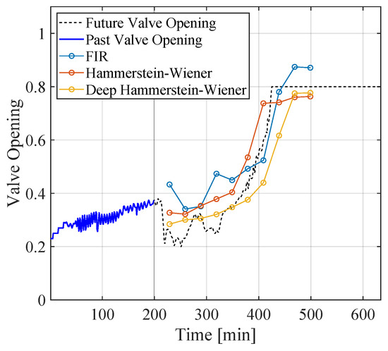
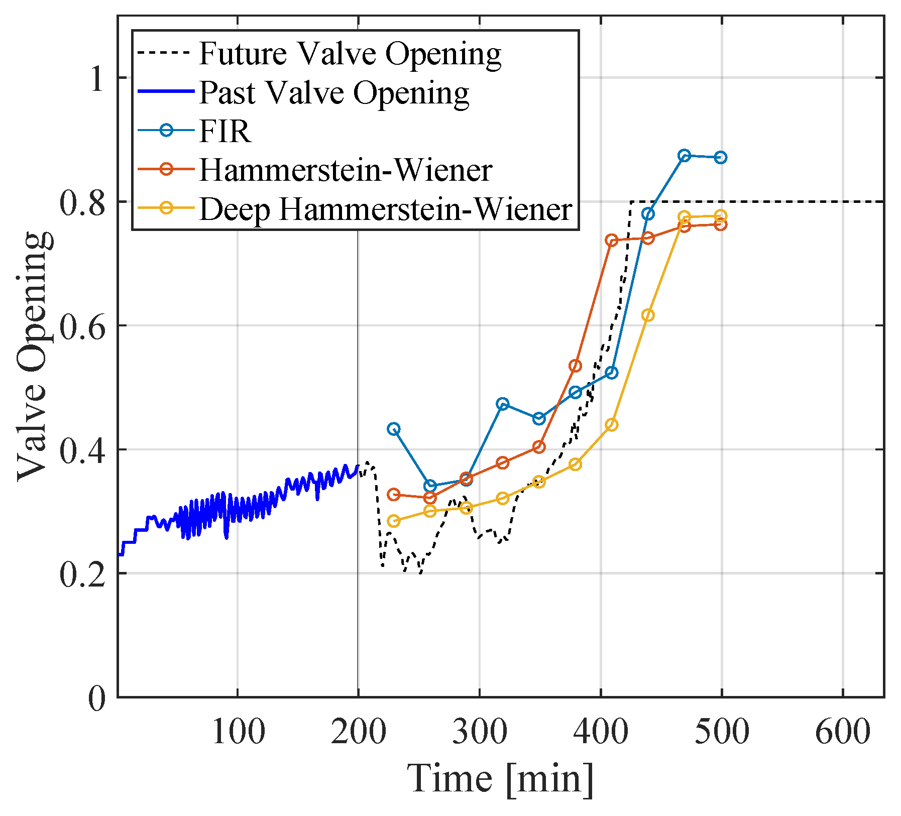
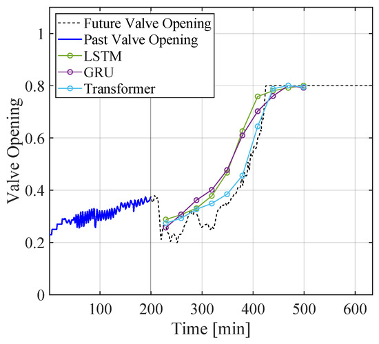
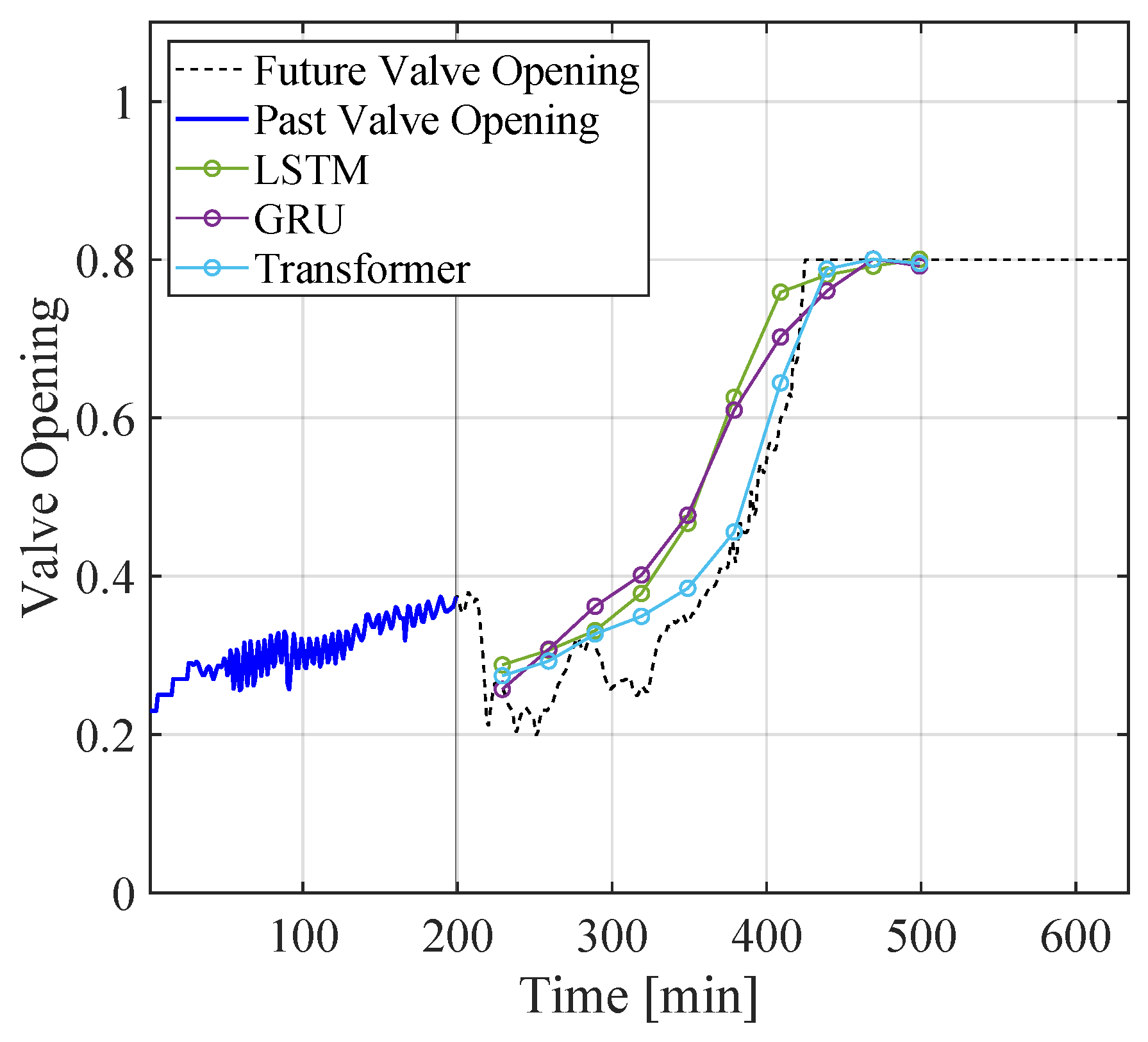
Figure 7 and Figure 8 show representative prediction results on the validation dataset for each model.

Figure 7. Representative time-series prediction results of valve opening obtained by neural network-based models (FIR, HW, and deep HW).

Figure 8. Representative time-series prediction results of valve opening obtained by neural network-based models (LSTM, GRU, and Transformer).

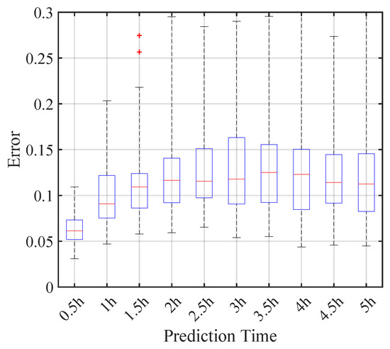
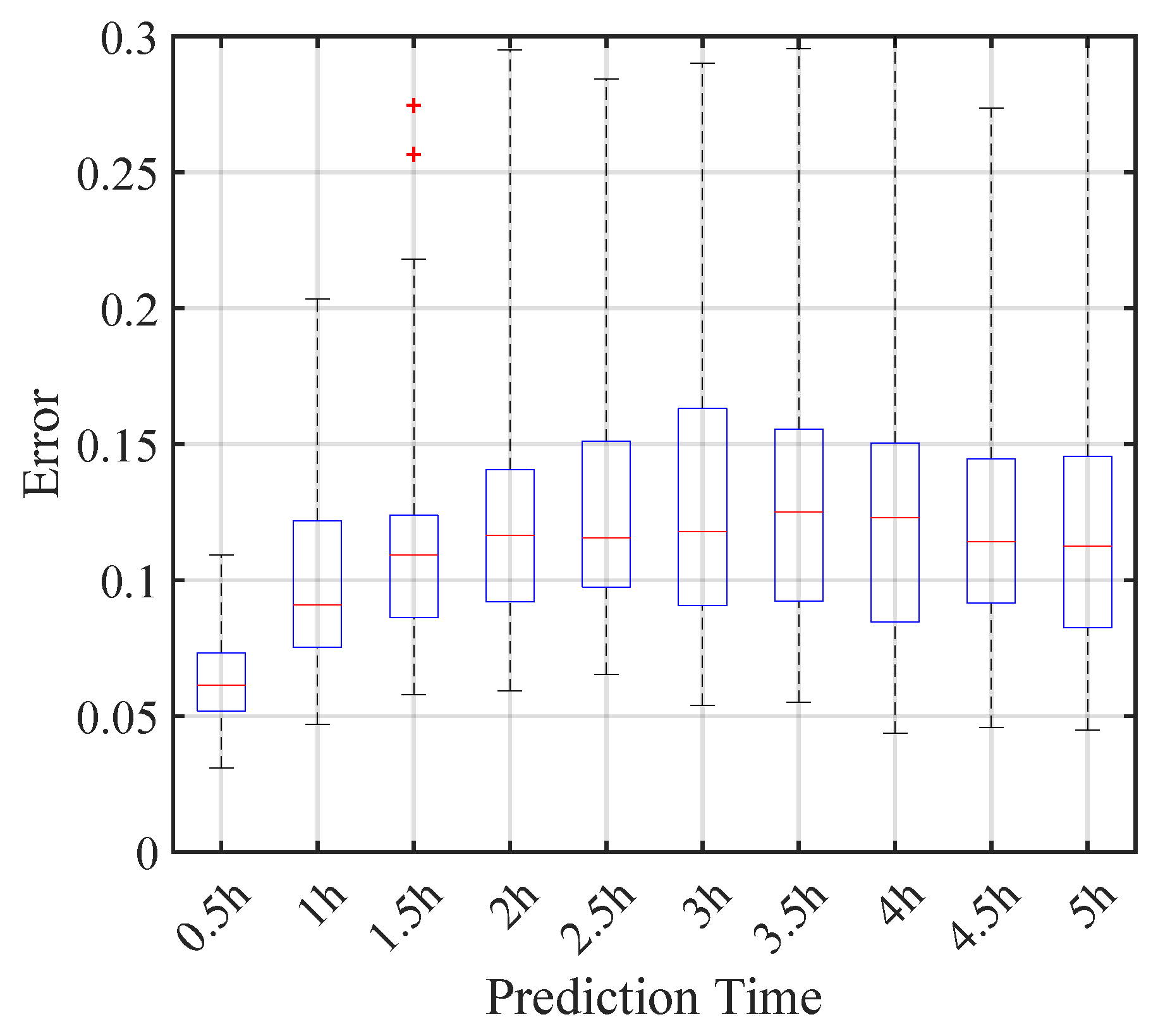
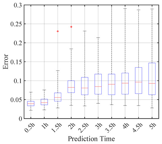
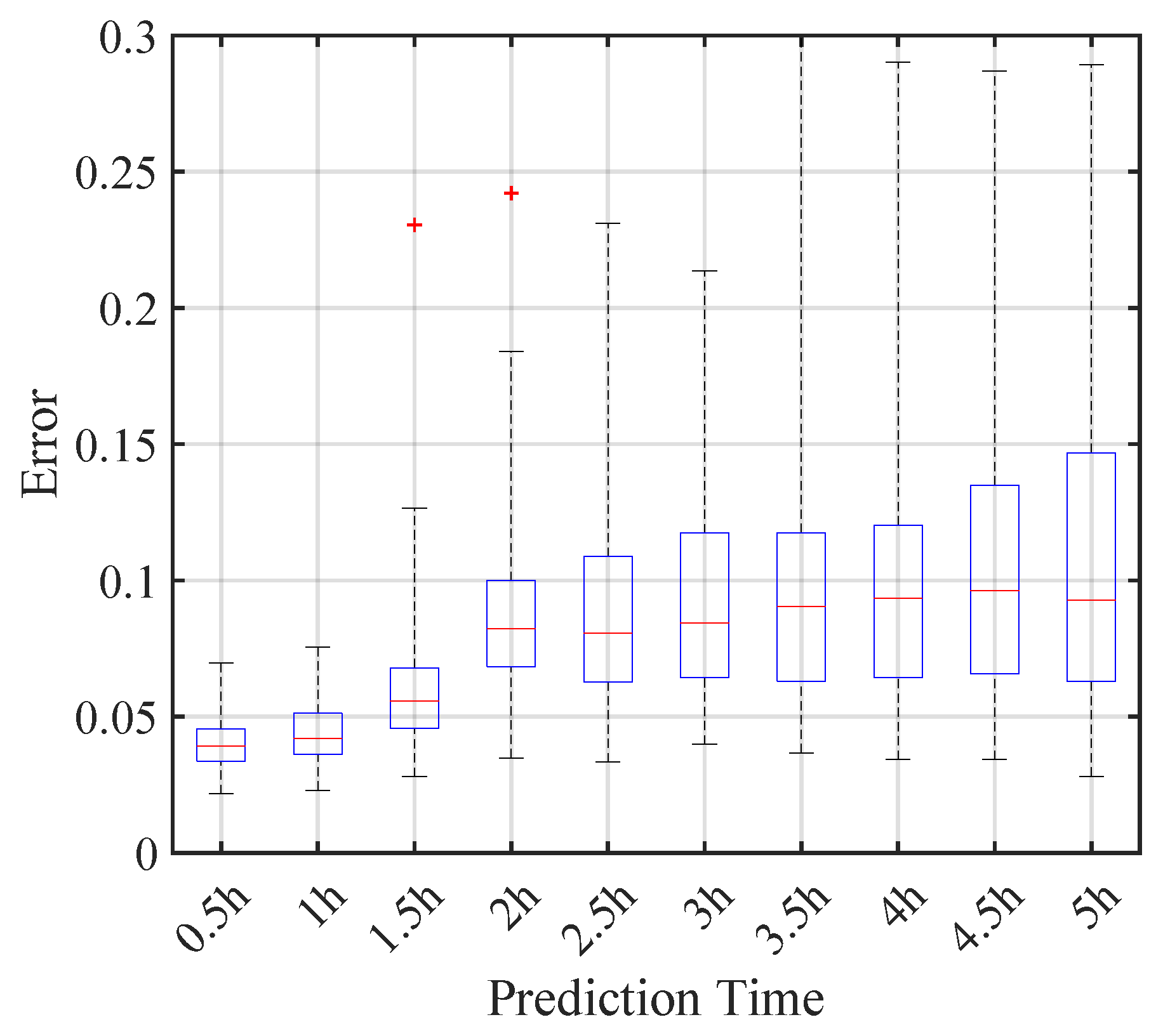
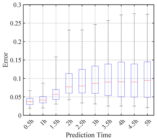
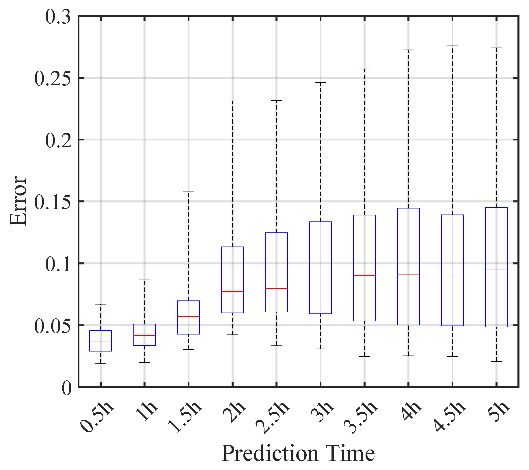
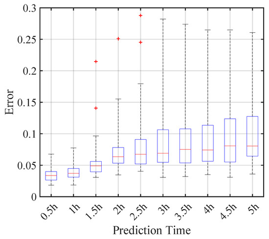
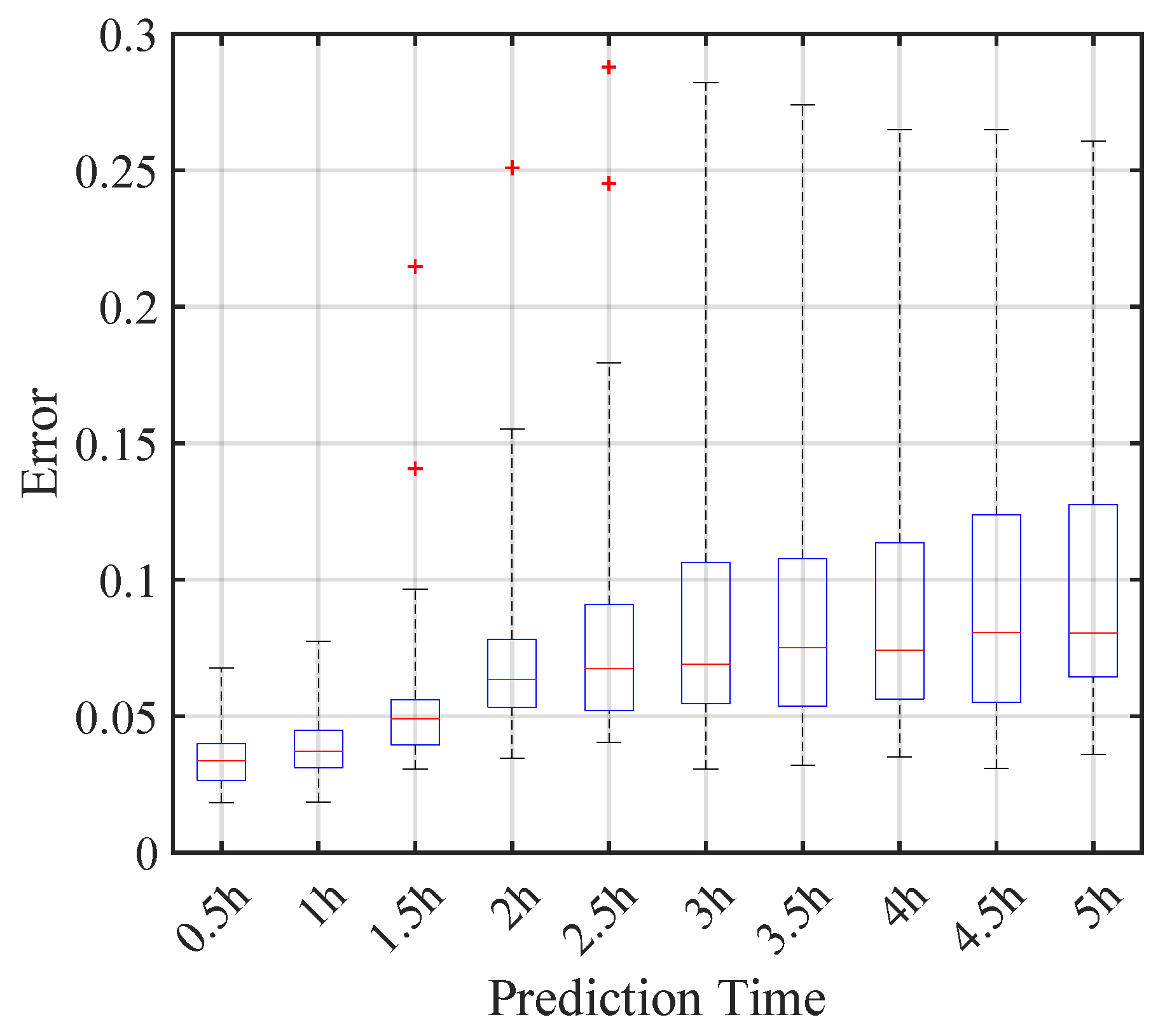
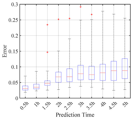
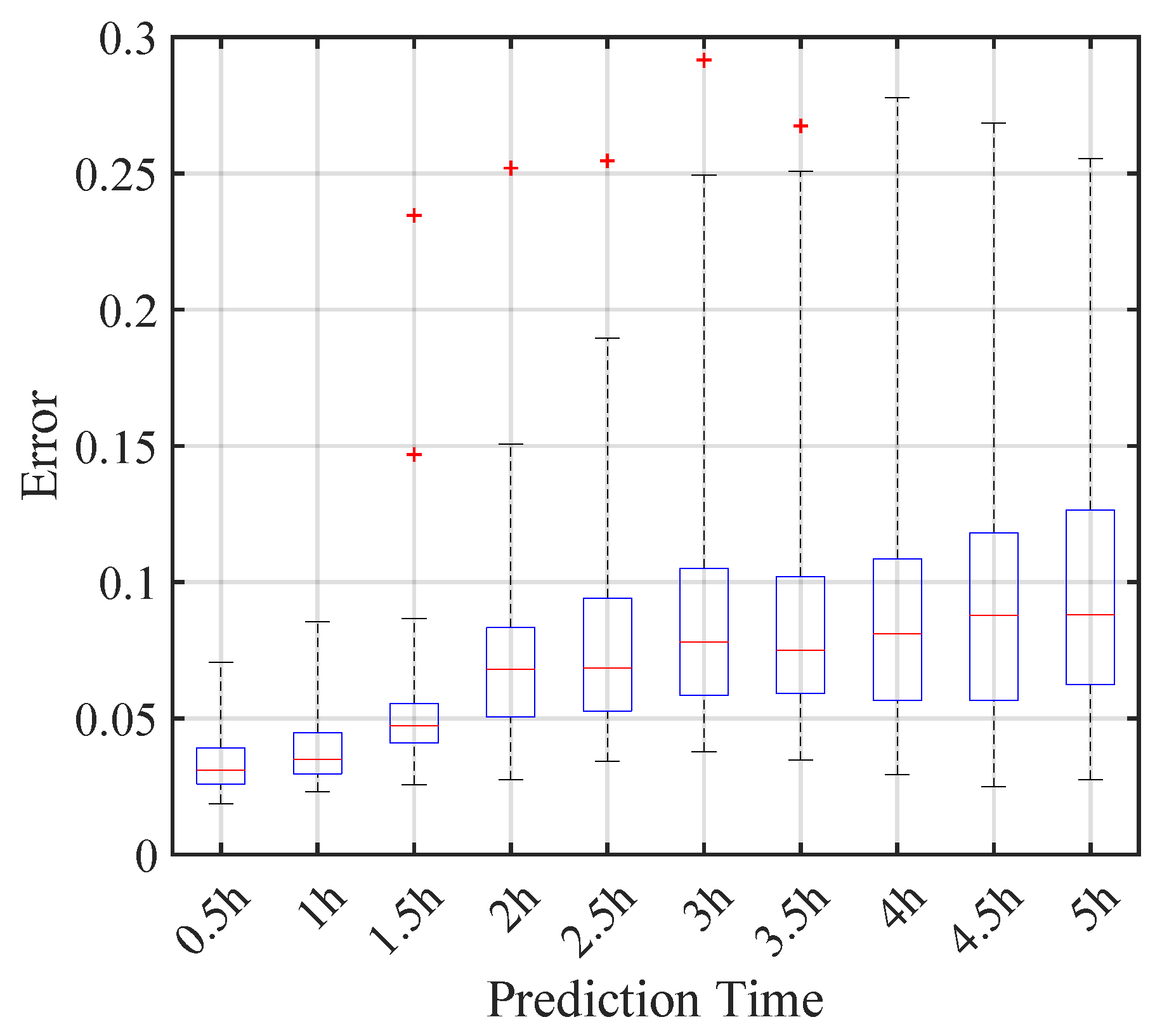
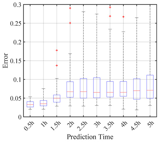
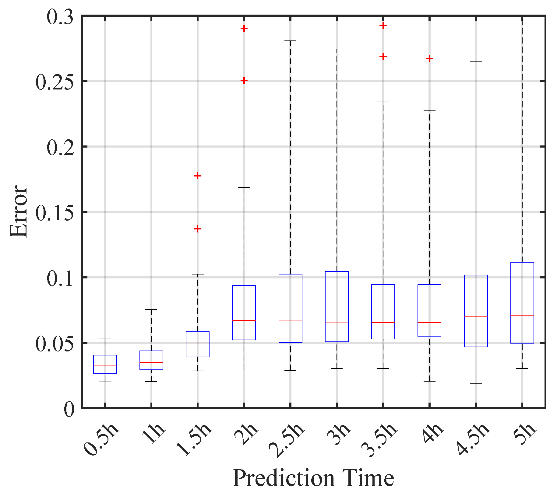
In the figure, the vertical line at 200 min indicates the current time step k. The solid blue line on the left side of the vertical line represents the historical valve opening, while the black dashed line on the right side represents the ground-truth valve opening to be predicted. The predicted valve openings obtained by the four models are compared with the ground truth. Figure 9, Figure 10, Figure 11, Figure 12, Figure 13 and Figure 14 are boxplots showing the prediction errors for each model.

Figure 9. Prediction errors of the FIR model for different prediction horizons.

Figure 10. Prediction errors of the HW model for different prediction horizons.

Figure 11. Prediction errors of the deep HW model for different prediction horizons.

Figure 12. Prediction errors of the LSTM model for different prediction horizons.

Figure 13. Prediction errors of the GRU model for different prediction horizons.

Figure 14. Prediction errors of the Transformer-based model for different prediction horizons.

The whiskers indicate the data range, the lower box edge represents the first quartile, the upper box edge represents the third quartile, and the red line indicates the median. The red plus symbols denote outliers. In these figures, the error shown on the vertical axis is defined as follows:

$$e=\sqrt{{\displaystyle \frac{1}{N}}\sum _{k=1}^N{\left(y_k-{\widehat{y}}_k\right)}^2},$$

(42)

where $y_k$ and ${\widehat{y}}_k$ represent the true valve opening and the predicted valve opening, respectively, and N denotes the number of segments in a single operation dataset. The results show that the error of the FIR model was larger than that of the other models, and the error increased as the prediction horizon increased.

The results presented in Table 3 indicate that the Transformer-based model achieves the best predictive performance on the validation dataset among all compared models. Furthermore, the box plots of prediction errors for each forecast horizon shown in Figure 14 reveal that the advantage of the Transformer becomes more pronounced as the prediction horizon increases. In particular, for long-term predictions (up to 5 h ahead), the Transformer yields smaller prediction errors compared with the other models. This tendency suggests that the Transformer is capable of effectively capturing long-term dependencies in the time series. Such a property is considered to contribute to its superior performance observed in Table 3.

5. Discussion

5.1. Effect of Nonlinearity in Valve Opening Prediction

The results indicate that linear modeling using the FIR model is insufficient for accurately predicting valve opening behavior over long prediction horizons. The observed increase in prediction error with respect to the prediction horizon suggests that the valve dynamics exhibit pronounced nonlinear characteristics, which cannot be adequately captured by linear models alone.

5.2. Contribution of Physical Variables Beyond Autoregression

The input vector used in this study includes the past history of the valve opening, which is also the output variable to be predicted. This configuration introduces an autoregressive component into the model, and thus raises the question of how much of the predictive performance is attributed to the valve opening itself versus other physical variables.

To clarify this point, an ablation study was conducted using two modified input settings. In the first setting (“Only Valve”), all input variables except the valve opening were replaced with zero, so that the model relies solely on the past valve opening. In the second setting (“Without Valve”), the valve opening in the input was replaced with zero, so that the prediction is based only on the remaining physical variables.

Table 4 summarizes the prediction performance of the Transformer-based model under these conditions. When only the valve opening is used as input, the prediction accuracy deteriorates significantly, yielding negative $R^2$ values for both training and validation datasets. This result indicates that the past valve opening alone is insufficient to explain the future system behavior.

Table 4. Prediction performance of the Transformer model under different input configurations on the training and validation datasets.

	Training			Validation
Model	RMSE	MAE	R2	RMSE	MAE	R2
Transformer (Full)	$0.061$	$0.037$	$0.906$	$0.083$	$0.046$	$0.829$
Transformer (Only Valve)	$0.308$	$0.239$	$-1.346$	$0.312$	$0.244$	$-1.406$
Transformer (Without Valve)	$0.082$	$0.049$	$0.833$	$0.093$	$0.054$	$0.788$

In contrast, when the valve opening is excluded from the input, the model still maintains relatively high prediction accuracy ($R^2=0.788$ on the validation dataset), although the performance is slightly degraded compared to the full-input model. This suggests that the physical variables contain substantial information relevant to the prediction of valve opening.

Overall, these results demonstrate that the proposed model does not rely solely on autoregressive information from the valve opening, but instead effectively utilizes the underlying physical variables to capture the system dynamics. This supports the validity of the modeling approach in representing the behavior of the plant beyond simple autoregressive prediction.

5.3. Practical Feasibility

To evaluate the computational efficiency of the models, the inference time per prediction step was measured. The results are summarized in Table 5.

Table 5. Inference time per prediction step for each model.

Model	Mean [ms]	Std [ms]
FIR	$2.1664$	$0.4320$
HW	$2.6719$	$0.4239$
Deep HW	$2.9401$	$0.4830$
LSTM	$5.0566$	$0.6800$
GRU	$3.3310$	$0.4515$
Transformer	$6.0512$	$1.3944$

As shown in Table 5, all models require only a few milliseconds per prediction step. Although differences in computational cost can be observed among the models, the overall inference time remains sufficiently small for practical use. Since model training is performed offline, the computational cost during operation is limited to forward inference, which is sufficiently lightweight for deployment on edge computing devices. Once deployed, the predicted valve opening can be presented to plant operators as a decision-support indicator. As described in Section 2, the prediction results can be used for planning operational actions such as waste feeding and resource allocation.

For example, as shown in Figure 8, the model predicts that the valve opening will exceed a certain threshold approximately five hours in advance. This enables operators to initiate necessary preparations ahead of time, which is sufficiently accurate for practical operational planning. It should be noted that the proposed model is not intended to directly control the switching operation, but rather to support human decision-making by providing advanced information. Therefore, prediction errors do not directly translate into control errors, but instead affect the amount of lead time available for preparation. From this perspective, the prediction horizon achieved in this study is considered sufficient to support stable and timely operational decisions.

5.4. Statistical Significance of Model Comparison

To assess whether the performance differences between models are statistically significant, the Wilcoxon signed-rank test was conducted for the prediction errors. The results are summarized in Table 6.

Table 6. Wilcoxon signed-rank test results for mean absolute error (MAE). Significance is determined at the 5% level ($p<0.05$).

Comparison	p-Value	Significant
FIR vs. Transformer	$1.34\times {10}^{-8}$	Yes
HW vs. Transformer	$2.31\times {10}^{-5}$	Yes
DeepHW vs. Transformer	$4.21\times {10}^{-3}$	Yes
LSTM vs. Transformer	$7.18\times {10}^{-2}$	No
GRU vs. Transformer	$2.24\times {10}^{-2}$	Yes

These results indicate that the Transformer model achieves statistically significant improvements over most baseline models in terms of MAE. In particular, significant differences are observed when compared with FIR, HW, DeepHW, and GRU models. On the other hand, the difference between the Transformer and LSTM models is not statistically significant at the 5% level. This suggests that the performance of these two models is comparable under the current experimental conditions. Further investigation, such as increasing the amount of training data or conducting additional validation, may be required to more clearly distinguish their performance.

5.5. Limitations and Practical Considerations

This study has several limitations related to dataset size, validation strategy, and robustness.

First, although the dataset used in this study was updated to include a larger number of operational samples compared to the initial experimental setting, the overall dataset size is still limited relative to typical large-scale learning scenarios. This may affect the generalization performance, particularly for deep learning models with a large number of parameters. Increasing the amount and diversity of data remains an important direction for future work.

Second, a fixed training–validation split was adopted for all models to ensure a consistent and fair comparison under the same experimental conditions. While K-fold cross-validation and external test sets are commonly used to evaluate generalization performance, they were not employed in this study in order to avoid excessive optimization for a specific dataset and to maintain a unified evaluation framework across different model structures.

Third, the dataset used in this study was obtained from a single plant. However, the intended application assumes that a separate model is constructed for each plant due to differences in equipment characteristics and operating conditions. Therefore, the use of a single-plant dataset is consistent with the practical deployment scenario rather than a limitation of the modeling framework itself.

Finally, this study does not explicitly evaluate robustness under distribution shifts, regime-specific performance, or sensitivity to dataset size. These aspects are important for real-world deployment, as plant operation conditions may vary depending on seasonal factors and operational strategies. Extending the analysis to include these perspectives, such as learning curve analysis and regime-based evaluation, is left for future work.

6. Conclusions

In this study, several nonlinear system identification approaches were investigated to construct prediction models for the operation of a gasification-based waste treatment plant. The models were trained and validated using actual operational data obtained from an industrial facility. The results demonstrate that incorporating nonlinear components is essential for accurately capturing the complex dynamics of the system, particularly for long-term valve opening prediction. Compared with the linear FIR model, the nonlinear models consistently achieved improved prediction accuracy, highlighting the importance of nonlinear modeling in complex industrial processes. Furthermore, the comparative analysis across different model structures, including block-oriented models and neural network-based approaches, indicates that advanced models can provide competitive and, in many cases, superior predictive performance. Statistical significance testing further supports these findings, confirming that several of the observed performance improvements are not due to random variation. Overall, the results suggest that nonlinear and data-driven modeling approaches provide a promising framework for supporting operational planning in gasification-based waste treatment systems.

7. Future Work

7.1. Model Interpretability

Interpretability is an important aspect for practical deployment, especially in industrial applications. In this study, interpretability is partially investigated through ablation analysis, which provides qualitative insights into the contribution of input variables. While block-oriented models such as the HW model offer a structurally interpretable framework, and Transformer models provide attention mechanisms that may reflect temporal dependencies, a detailed analysis of internal model representations is beyond the scope of this study. A more systematic investigation of model interpretability, including parameter-level analysis and attention-based interpretation, is left for future work.

7.2. Comparison with Advanced Transformer Variants

In recent years, several advanced Transformer-based architectures for time-series prediction, such as the Temporal Fusion Transformer (TFT) [21] and Autoformer [23], have been proposed. These models introduce additional mechanisms, including variable selection, decomposition, and improved attention structures, to enhance predictive performance.

In this study, the applicability of the baseline Transformer model to industrial operation data is evaluated under a unified experimental setting. From this perspective, the objective is not to exhaustively compare all possible Transformer variants, but to establish a clear reference point by assessing the effectiveness of the standard architecture. The results demonstrate that the Transformer-based approach provides competitive performance compared with conventional models, indicating its suitability for the target problem. Based on this finding, extending the analysis to more advanced Transformer variants such as TFT and Autoformer is considered an important direction for future work.

References

- Egusa, T.; Terasawa, Y.; Suzuki, W.; Masuyama, S.; Hayashi, K.; Tamura, H. Introduction of Remote Monitoring and Operational Support Systems Aiming at Optimal Management of Waste-to-Energy Plants. Mitsubishi Heavy Ind. Tech. Rev. 2020, 57, e572040. [Google Scholar]
- Kadlec, P.; Gabrys, B.; Strandt, S. Data-Driven Soft Sensors in the Process Industry. Comput. Chem. Eng. 2009, 33, 795–814. [Google Scholar] [CrossRef] [Scilit]
- Ljung, L. Perspectives on system identification. Annu. Rev. Control 2010, 34, 1–12. [Google Scholar] [CrossRef] [Scilit]
- Liu, Z.; Guo, H.; Zhang, Y.; Zuo, Z. A Comprehensive Review of Wind Power Prediction Based on Machine Learning: Models, Applications, and Challenges. Energies 2025, 18, 350. [Google Scholar] [CrossRef] [Scilit]
- Arena, U. Process and technological aspects of municipal solid waste gasification. A review. Waste Manag. 2012, 32, 625–639. [Google Scholar] [CrossRef] [Scilit] [PubMed]
- Box, G.; Jenkins, G. Time Series Analysis: Forecasting and Control; Holden-Day Series in Time Series Analysis and Digital Processing, Holden-Day; John Wiley & Sons: Hoboken, NJ, USA, 1976. [Google Scholar]
- Hyndman, R.; Athanasopoulos, G. Forecasting: Principles and Practice; OTexts: Melbourne, Australia, 2018. [Google Scholar]
- Yang, Y.; Shahbeik, H.; Shafizadeh, A.; Rafiee, S.; Hafezi, A.; Du, X.; Pan, J.; Tabatabaei, M.; Aghbashlo, M. Predicting municipal solid waste gasification using machine learning: A step toward sustainable regional planning. Energy 2023, 278, 127881. [Google Scholar] [CrossRef] [Scilit]
- Nelles, O. Nonlinear System Identification: From Classical Approaches to Neural Networks and Fuzzy Models; Engineering Online Library; Springer: Berlin/Heidelberg, Germany, 2001. [Google Scholar]
- Billings, S. Nonlinear System Identification: NARMAX Methods in the Time, Frequency, and Spatio-Temporal Domains; Matematicas (E-libro–2014/09); Wiley: Hoboken, NJ, USA, 2013. [Google Scholar]
- Pearson, R.K. Nonlinear input/output modelling. J. Process Control 1995, 5, 197–211. [Google Scholar] [CrossRef] [Scilit]
- Ascher, S.; Sloan, W.; Watson, I.; You, S. A comprehensive artificial neural network model for gasification process prediction. Appl. Energy 2022, 320, 119289. [Google Scholar] [CrossRef] [Scilit]
- Alfarra, F.; Ozcan, H.K.; Cihan, P.; Ongen, A.; Guvenc, S.Y.; Ciner, M.N. Artificial intelligence methods for modeling gasification of waste biomass: A review. Environ. Monit. Assess. 2024, 196, 309. [Google Scholar] [CrossRef] [Scilit] [PubMed]
- Sun, C.; Ai, L.; Liu, T. The PSO-ANN modeling study of highly valuable material and energy production by gasification of solid waste: An artificial intelligence algorithm approach. Biomass Convers. Biorefinery 2024, 14, 2173–2184. [Google Scholar] [CrossRef] [Scilit]
- Tang, J.; Wang, T.; Xia, H.; Cui, C. An Overview of Artificial Intelligence Application for Optimal Control of Municipal Solid Waste Incineration Process. Sustainability 2024, 16, 2042. [Google Scholar] [CrossRef] [Scilit]
- Ahmed, A.; del Rio-Chanona, E.A.; Mercangoz, M. Comparative study of machine learning and system identification for process systems engineering dynamics. Ind. Eng. Chem. Res. 2025, 64, 4450–4478. [Google Scholar] [CrossRef] [Scilit] [PubMed]
- Bai, S.; Kolter, J.Z.; Koltun, V. An Empirical Evaluation of Generic Convolutional and Recurrent Networks for Sequence Modeling. arXiv 2018. http://arxiv.org/abs/1803.01271.
- Paszke, A.; Gross, S.; Massa, F.; Lerer, A.; Bradbury, J.; Chanan, G.; Killeen, T.; Lin, Z.; Gimelshein, N.; Antiga, L.; et al. PyTorch: An Imperative Style, High-Performance Deep Learning Library. In Proceedings of the Advances in Neural Information Processing Systems; Wallach, H., Larochelle, H., Beygelzimer, A., d’Alché-Buc, F., Fox, E., Garnett, R., Eds.; Curran Associates, Inc.: Red Hook, NY, USA, 2019; Volume 32. [Google Scholar]
- Vaswani, A.; Shazeer, N.; Parmar, N.; Uszkoreit, J.; Jones, L.; Gomez, A.N.; Kaiser, L.u.; Polosukhin, I. Attention is All you Need. In Proceedings of the Advances in Neural Information Processing Systems; Guyon, I., Luxburg, U.V., Bengio, S., Wallach, H., Fergus, R., Vishwanathan, S., Garnett, R., Eds.; Curran Associates, Inc.: Red Hook, NY, USA, 2017; Volume 30. [Google Scholar]
- Qin, Y.; Song, D.; Chen, H.; Cheng, W.; Jiang, G.; Cottrell, G. A Dual-Stage Attention-Based Recurrent Neural Network for Time Series Prediction. arXiv 2017. http://arxiv.org/abs/1704.02971.
- Lim, B.; Arık, S.Ö.; Loeff, N.; Pfister, T. Temporal Fusion Transformers for interpretable multi-horizon time series forecasting. Int. J. Forecast. 2021, 37, 1748–1764. [Google Scholar] [CrossRef] [Scilit]
- Li, S.; Jin, X.; Xuan, Y.; Zhou, X.; Chen, W.; Wang, Y.X.; Yan, X. Enhancing the Locality and Breaking the Memory Bottleneck of Transformer on Time Series Forecasting. arXiv 2020. http://arxiv.org/abs/1907.00235.
- Wu, H.; Xu, J.; Wang, J.; Long, M. Autoformer: Decomposition Transformers with Auto-Correlation for Long-Term Series Forecasting. In Proceedings of the Advances in Neural Information Processing Systems; Ranzato, M., Beygelzimer, A., Dauphin, Y., Liang, P., Vaughan, J.W., Eds.; Curran Associates, Inc.: Red Hook, NY, USA, 2021; Volume 34, pp. 22419–22430. [Google Scholar]
- He, K.; Zhang, X.; Ren, S.; Sun, J. Deep Residual Learning for Image Recognition. In Proceedings of the 2016 IEEE Conference on Computer Vision and Pattern Recognition (CVPR), Los Alamitos, CA, USA, 27–30 June 2016; pp. 770–778. [Google Scholar] [CrossRef] [Scilit]
- Ba, J.L.; Kiros, J.R.; Hinton, G.E. Layer Normalization. arXiv 2016. http://arxiv.org/abs/1607.06450.
- Ławryńczuk, M.; Zarzycki, K. LSTM and GRU type recurrent neural networks in model predictive control: A Review. Neurocomputing 2025, 632, 129712. [Google Scholar] [CrossRef] [Scilit]
Disclaimer/Publisher’s Note: The statements, opinions and data contained in all publications are solely those of the individual author(s) and contributor(s) and not of MDPI and/or the editor(s). MDPI and/or the editor(s) disclaim responsibility for any injury to people or property resulting from any ideas, methods, instructions or products referred to in the content. |
© 2026 by the authors. Licensee MDPI, Basel, Switzerland. This article is an open access article distributed under the terms and conditions of the Creative Commons Attribution (CC BY) license.