Braking Control Strategy for Battery Electric Buses Based on Dynamic Load Estimation

Abstract

In real-world operation, battery electric buses often encounter conditions with significant and rapid load variations. To improve regenerative braking energy recovery efficiency under such dynamic load conditions, this paper proposes a braking control strategy based on dynamic load estimation. First, a load estimation method based on a time-varying interactive multiple-model unscented Kalman filter (TVIMM-UKF) is developed by leveraging the vehicle longitudinal dynamics model and IMU sensor data, achieving high-accuracy online load estimation. Second, a multi-objective constrained optimization model is established, and an improved artificial bee colony algorithm is introduced to realize optimal brake force distribution under time-varying loads. Based on this, a regenerative braking control strategy is designed by incorporating motor characteristics and system-level operational constraints, enabling precise adjustment of braking torque across the full load range. Finally, simulation studies are conducted under two typical driving cycles, CHTC-B and C-WTVC, to verify the effectiveness of the proposed strategy. The results show that under dynamic load conditions, the proposed strategy can effectively improve braking energy recovery efficiency in both driving cycles.

1. Introduction

With the ongoing global shift in energy structures and the implementation of increasingly stringent environmental policies, battery electric vehicles (BEVs) have emerged as a key direction for the transformation and upgrading of the automotive industry, owing to their remarkable advantages of zero emissions, low energy consumption, and reduced noise [1]. Among them, battery electric buses (BEBs), as an essential component of public transportation, play a vital role in promoting sustainable mobility and advancing green transportation initiatives [2,3]. Within BEBs, the braking control system is not only responsible for ensuring vehicle deceleration and safety but also serves as a critical mechanism for regenerative braking, thereby contributing significantly to energy recovery [4,5].

Research on braking control strategies encompasses several key aspects, primarily including brake force distribution, braking stability control, and regenerative braking [6,7,8]. In recent years, numerous scholars have proposed innovative methods in the field of braking system control. Brake force distribution directly affects vehicle safety, stability, and energy efficiency. By optimizing the allocation ratio between the front and rear axles, vehicles can achieve stable and efficient braking performance under varying operating conditions [9]. For example, Wang designed a hierarchical braking precision control algorithm that improves control accuracy and energy recovery efficiency by considering the effects of multiple resistive forces and applying compensatory control of hydraulic braking torque, thereby eliminating the need for an explicit torque distribution process [10]. Liu et al. proposed a dynamic braking force distribution strategy based on a PID algorithm, in which a PID controller targeting the desired slip ratio is employed to dynamically adjust the braking force distribution coefficient between the front and rear axles, significantly enhancing braking efficiency and driving stability [11]. Li et al. coordinated motor braking and hydraulic braking under different operating modes based on an ideal braking force distribution strategy, and further proposed an anti-lock braking strategy relying solely on motor torque regulation. This approach avoids interference between hydraulic and motor braking, effectively achieves the target braking intensity, and maintains vehicle stability [12]. Wang et al. developed a braking force control strategy based on explicit nonlinear model predictive control (ENMPC) to replace conventional ABS schemes, and employed the grey wolf optimization algorithm to rationally allocate mechanical and electrical braking forces, thereby improving braking performance under varying road conditions [13]. Liu et al. established a seven-degree-of-freedom full-vehicle dynamics model and formulated an adaptive braking force distribution control strategy based on the I-curve and the Economic Commission for Europe (ECE) regulations. The results demonstrate that the proposed strategy exhibits superior adaptability to complex and varying driving conditions [14].

In the field of regenerative braking research, Faghihian et al. proposed an Eco-Regen system that employs a continuously variable transmission ratio to maximize energy recovery during braking events. A fuzzy logic controller is further adopted to select the optimal transmission ratio within the Eco-Regen system, and the results demonstrate a significant increase in total recovered energy [15]. Li et al. introduced a game-theory-based optimization strategy for regenerative braking control in electric vehicles, which enhances energy recovery, braking stability, and ride comfort throughout the entire braking process [16]. Cai et al. developed an improved model predictive control strategy that ensures smooth and safe regenerative braking while improving energy recovery efficiency. Simulation and real-vehicle experiments indicate that the proposed method exhibits superior real-time performance and adaptability under complex driving conditions, with a significantly reduced average computation time [17]. Qiu et al. optimized the regenerative braking energy recovery system of pure electric vehicles based on driving styles and established an IDP-BLSTM-based management and control strategy. Road tests verified that the proposed approach satisfies the personalized requirements of different drivers and achieves efficient energy recovery while enhancing safety and driving experience [18]. Zhou et al. addressed the coupling effect between braking jerk and energy recovery efficiency by employing a multi-objective cuckoo search algorithm to jointly optimize regenerative braking torque and gear-shift timing, resulting in a 47.06% improvement in energy recovery rate [19].

It can be observed that current research on braking control strategies for BEVs largely overlooks the critical impact of load as a dynamic variable on overall vehicle braking performance. In the specific application scenario of BEBs, wide variations in load result in significant changes in vehicle mass, center of gravity position, and the dynamic distribution of front and rear axle loads, necessitating braking control strategies with high adaptability and robustness. Under different load conditions, the vehicle’s inertial characteristics, braking requirements, and regenerative braking potential all vary, imposing higher demands on the real-time responsiveness and precise adjustment capabilities of the braking control system.

To overcome the aforementioned limitations, this study proposes a braking control strategy for battery electric buses based on dynamic load estimation. First, to address the poor transient performance of traditional methods under frequent stop-and-go conditions, which rely heavily on longitudinal vehicle dynamics parameters, an IMU-enhanced dynamic model incorporating high-frequency acceleration measurements is introduced. The longitudinal acceleration and gravitational components provided by the IMU effectively compensate for the information insufficiency of the dynamics model at low speeds and during mild acceleration or deceleration, thereby significantly improving the observability and real-time performance of load estimation. Building on this, a dynamic load estimation method using a TVIMM-UKF is developed. By constructing parallel models of vehicle dynamics and IMU observation, and employing model probability updates with state fusion mechanisms, the proposed method achieves adaptive load estimation. This approach resolves the inherent trade-off in single-model estimators between steady-state accuracy and transient responsiveness, ensuring high estimation accuracy and robustness under complex operating conditions.

Second, based on the real-time estimated load, a multi-constraint braking force distribution model is formulated, integrating the I-curve, ECE regulations, and motor characteristics into a unified optimization framework. To avoid the drawbacks of traditional optimization algorithms—such as susceptibility to local optima and low convergence efficiency—an improved Artificial Bee Colony (ABC) algorithm incorporating Bernoulli chaotic mapping is employed to obtain the optimal front–rear braking force distribution. Furthermore, a regenerative braking control strategy is designed by jointly considering motor constraints, battery State of Charge (SoC) limits, and braking-intensity boundaries, thereby enabling precise torque regulation and maximizing energy recovery under dynamically varying load conditions.

The main contributions of this study can be summarized as follows:

• A dynamic load estimation method based on TVIMM-UKF is developed to improve estimation accuracy under varying passenger loading conditions.
• An improved ABC optimization algorithm is introduced to determine the optimal brake force distribution considering dynamic load variations.
• The proposed strategy is validated under CHTC-B and C-WTVC driving cycles, demonstrating improved regenerative braking efficiency and SoC performance.

The structure of this paper is as follows. Section 2 presents real-time vehicle load estimation based on the TVIMM-UKF algorithm. In Section 3, under the constraints of the ideal brake force distribution curve and ECE regulations, an improved Artificial Bee Colony algorithm is proposed for optimal brake force distribution, and a regenerative braking control strategy that integrates motor characteristics and system operating constraints is developed. Section 4 introduces the relevant parameters of the studied vehicle model and the simulation platform, followed by the presentation of simulation results. Finally, Section 5 provides a summary of the paper.

2. Vehicle Load Estimation Using the TVIMM-UKF Algorithm

This section presents the vehicle dynamic load estimation method. A longitudinal dynamics model and an IMU-enhanced dynamic model are established, and the TVIMM-UKF algorithm is employed to estimate the bus load online, providing real-time input for the subsequent braking control strategy.

2.1. Formulation and Discretization of Longitudinal Vehicle Dynamics

To achieve accurate online identification of the vehicle load, a longitudinal dynamic model is first established to capture the actual operating characteristics of the vehicle, where the balance between the driving force and various resistance components is comprehensively considered.

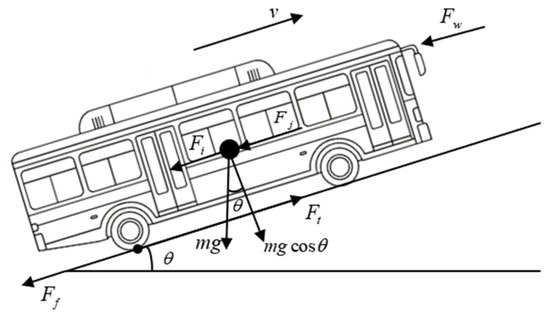
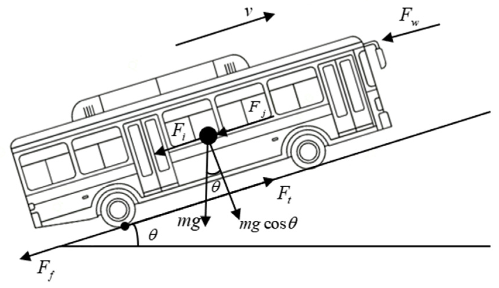
The longitudinal vehicle dynamics model is shown in Figure 1. Where $F_t$ is the driving force, $F_f$ is the rolling resistance, $F_w$ is the aerodynamic drag, $F_j$ is the acceleration resistance, $F_i$ is the grade resistance, $v$ is the longitudinal vehicle speed, $m$ is the vehicle mass, $g$ is the gravitational acceleration, and $\theta$ is the road slope.

Figure 1. Longitudinal dynamics model of the vehicle.

According to Newton’s second law, the longitudinal force balance equation of the vehicle is expressed as [20]

$$m{\displaystyle \frac{d\nu }{dt}}={\displaystyle \frac{T_m{i}_g\eta }{r}}-f_{r}mg\cos \theta -{\displaystyle \frac{1}{2}}{C}_{d}A\rho {\nu }^2-mg\sin \theta$$

(1)

where $T_m$ represents the motor output torque, $i_g$ the total transmission ratio of the drivetrain, $\eta$ the drivetrain efficiency,$r$ the wheel rolling radius, $f_r$ the rolling resistance coefficient, $C_d$ the aerodynamic drag coefficient, $A$ the vehicle frontal area, and $\rho$ the air density.

Since urban buses usually operate on roads with relatively small gradients, the road slope angle $\theta$ is assumed to be small. Therefore, the approximations $\cos \theta \approx 1$ and $\sin \theta \approx \theta$ can be applied to simplify the model. Under this assumption, Equation (1) can be rewritten as

$$m{\displaystyle \frac{d\nu }{dt}}={\displaystyle \frac{T_m{i}_g\eta }{r}}-f_{r}mg-{\displaystyle \frac{1}{2}}{C}_{d}A\rho {\nu }^2-mg\theta$$

(2)

By selecting the vehicle speed and the vehicle mass as the system state variables, with the vehicle speed serving as the measured output, the vehicle mass is treated as a slowly time-varying parameter and is included in the state vector for online estimation. Its time evolution is modeled as a random-walk process with zero mean, which allows the estimator to capture gradual variations caused by passenger loading changes under normal driving conditions. Based on this assumption, the time derivative of the vehicle mass is approximated as zero in the deterministic sense. The continuous-time state equation of the system can therefore be expressed as follows:

$$\left\{\begin{array}{c}\dot{v}={\displaystyle \frac{T_m{i}_g\eta }{rm}}-f_{r}g-{\displaystyle \frac{1}{2m}}{C}_{d}A\rho {\nu }^2-g\theta \\ \dot{m}=0\end{array}\right.$$

(3)

By applying the forward Euler method to discretize Equation (3), and assuming that the system noise and measurement noise are mutually independent zero-mean Gaussian white noises, denoted by $W_{1k}$ and $V_{1k}$, respectively, the model can be expressed in matrix form as follows.

$$\left[\begin{array}{c}{v}_k\\ m_k\end{array}\right]=\left[\begin{array}{c}{v}_{k-1}+\Delta t\left({\displaystyle \frac{T_{m,k-1}{i}_g\eta }{m_{k-1}r}}-f_{r}g-{\displaystyle \frac{C_{d}A\rho {v_{k-1}}^2}{2m_{k-1}}}-g\theta \right)\\ m_{k-1}\end{array}\right]+W_{1k}$$

(4)

The system measurement equation is given by

$$z_k=[1\hspace{1em}0]\left[\begin{array}{c}{v}_k\\ m_k\end{array}\right]+V_{1k}$$

(5)

2.2. Construction of an IMU-Enhanced Dynamic Model

The inertial measurement unit (IMU) integrated into the studied vehicle provides high-frequency longitudinal acceleration data. By incorporating this information, an IMU-enhanced dynamic model is constructed to improve the fidelity of the vehicle dynamics representation and support vehicle load estimation.

The measured accelerations along the slope direction and perpendicular to the slope direction are given as follows:

$$\left\{\begin{array}{c}{a}_{senx}=g\sin \theta +{\displaystyle \frac{dv}{dt}}\\ a_{senz}=g\cos \theta \end{array}\right.$$

(6)

By combining Equation (6) with Equation (1), the following expression is obtained:

$${\displaystyle \frac{T_m{i}_g\eta }{r}}-{\displaystyle \frac{1}{2}}{C}_{d}A\rho {\nu }^2=m\left(a_{senx}+f_r{a}_{senz}\right)$$

(7)

The vehicle mass is selected as the state variable:

$$x_k=M_k$$

(8)

The system state equation is expressed as follows:

$$x_{k+1}=x_k+W_{2k}$$

(9)

where $W_{2k}$ represents the process noise, which follows a zero-mean Gaussian distribution with covariance $Q$.

The observation equation is given by

$$z_k=H_k{x}_k+V_{2k}$$

(10)

2.3. The TVIMM-UKF Algorithm

The longitudinal vehicle dynamics considered in this study are inherently nonlinear. The extended Kalman filter (EKF) is a widely used method for nonlinear state estimation; however, it relies on a first-order Taylor series expansion to linearize the nonlinear state and measurement equations around the current mean and covariance. This approximation introduces linearization errors and only achieves first-order accuracy. In scenarios involving frequent stop-and-go operations and time-varying vehicle loads, such as electric bus applications, these limitations may degrade estimation accuracy and even lead to filter divergence.

To overcome these limitations, the unscented Kalman filter UKF is adopted as the core estimation algorithm. The UKF employs the unscented transformation (UT) to handle nonlinear state propagation without explicit linearization. Specifically, a set of deterministically selected sigma points is generated around the state mean to capture the underlying probability distribution. These sigma points are propagated through the nonlinear system dynamics, and the posterior mean and covariance are reconstructed via weighted statistics. This approach can accurately capture the posterior statistics up to the third order for Gaussian distributions, thereby significantly improving estimation accuracy and robustness under nonlinear conditions.

Load estimation methods based on the baseline longitudinal dynamic model and the IMU-enhanced dynamic model each exhibit distinct advantages and limitations. The former is straightforward to implement and relies on physically interpretable parameters, but it is sensitive to modeling inaccuracies and may exhibit poor transient performance under frequent acceleration and deceleration [21]. The latter incorporates acceleration measurements to rapidly capture load variations during dynamic maneuvers; however, it is susceptible to sensor noise and external disturbances [22]. In addition, since vehicle mass is a slowly varying parameter, its observability may be weakened under low-speed or quasi-steady driving conditions due to insufficient system excitation.

To leverage the complementary strengths of these two models and improve estimation performance under varying operating conditions, a time-varying interacting multiple model TVIMM framework is introduced and combined with the UKF to form the proposed TVIMM-UKF algorithm. Through probabilistic model interaction and adaptive weighting, the TVIMM framework dynamically adjusts the contribution of each model, enabling more accurate and robust estimation of the vehicle mass.

The TVIMM-UKF algorithm assumes that two state estimation models run in parallel within the system, collaboratively performing the task of inferring the system states through five functional modules [23].

(1)

Model Input Interaction

To enable information sharing between models and account for model transition probabilities, a Markov chain mechanism is employed to perform a weighted mixture of the state estimates from the previous time step.

The transition probability matrix between the two models at time step $k-1$ is defined as follows:

$$\pi =\left[\begin{array}{cc}{\pi }_{11}\left(k-1\right)& {\pi }_{12}\left(k-1\right)\\ {\pi }_{21}\left(k-1\right)& {\pi }_{22}\left(k-1\right)\end{array}\right]$$

(11)

where ${\pi }_{ij}(k-1)$ denotes the transition probability from model $i$ to model $j$. The $i\text{-}\mathrm{th}$ row of the matrix represents the probabilities that model $i$ at time step $k-1$ transitions to other models, while the $j\text{-}\mathrm{th}$ column represents the probabilities of other models transitioning to model $j$ at time step $k-1$.

The mixing probability from model $i$ to model $j$ is given by

$${\mu }_{ij}(k-1|k-1)={\displaystyle \frac{{\mu }_i(k-1){\pi }_{ij}(k-1)}{{\displaystyle \sum _{i=1}^2}{\mu }_i(k-1){\pi }_{ij}(k-1)}}$$

(12)

where ${\mu }_i(k-1)$ represents the probability of model $i$ at time step $k-1$.

The mixed initial state of model $j$ is given by

$${\widehat{x}}_j^0(\left.k-1\right|k-1)=\sum _{i=1}^2{\mu }_{ij}(k-1|k-1)·{\widehat{x}}_i(k-1\left|k-1\right.)$$

(13)

where $j=1,2$, and ${\widehat{x}}_i(k-1\left|k-1\right.)$ denotes the estimated state of model $i$ at time step $k-1$.

The mixed covariance of model $j$ is given by

$$\begin{array}{l}{P}_j^0(k-1\left|k-1\right.)={\displaystyle \sum _{i=1}^2}{\mu }_{ij}(k-1|k-1)·\\ \left\{P_i(k-1\left|k-1\right.)+[{\widehat{x}}_i(k-1\left|k-1\right.)-{\widehat{x}}_j^0(k-1\left|k-1\right.)]·\right.\\ \left.{[{\widehat{x}}_i(k-1\left|k-1\right.)-{\widehat{x}}_j^0(k-1\left|k-1\right.)]}^T\right\}\end{array}$$

(14)

where $P_i(k-1\left|k-1\right.)$ is the covariance matrix of model $i$ at time step $k-1$.

(2)

UKF Output

For each model $j$, the Unscented Kalman Filter (UKF) is used to perform nonlinear state prediction and update [24]. First, the model state is predicted, with the Kalman gain given by

$$K_j(k)=P_{xz,j}(k|k-1){\left[P_{z,j}(k|k-1)\right]}^{-1}$$

(15)

where $P_{xz}$ is the cross-covariance between the state and the measurement, and $P_z$ is the measurement covariance.

The state is then updated as

$${\widehat{x}}_j(k|k)={\widehat{x}}_j(k|k-1)+K_j(k)\left[z(k)-{\widehat{z}}_j(k|k-1)\right]$$

(16)

The covariance is updated as

$$P_j(k|k)=P_j(k|k-1)-K_j(k)P_{z,j}(k|k-1)K_j^T(k)$$

(17)

(3)

Model State Fusion

Bayesian posterior probability density estimation is employed to perform a weighted fusion of the state outputs from all models, yielding the overall system state estimate. The fused state and its covariance are given by

$$P(k|k)={[\sum _{j=1}^2{P}_j^{-1}(k|k)]}^{-1}$$

(18)

$$\widehat{x}(k|k)=P(k|k)·{[\sum _{j=1}^2{P}_j^{-1}(k|k)]}^{-1}·{\widehat{x}}_j(k|k)$$

(19)

This step fuses the target states to obtain the optimal estimate of the Bayesian posterior probability distribution.

(4)

Model Probability Update

The model probabilities are updated according to the likelihood of each model with respect to the fused state. For each model $j$, the likelihood of the fused state at the current time step is defined as

$${\mathsf{\Lambda }}_j(k)=N[{\widehat{x}}_j(k|k);\widehat{x}(k|k),P(k|k)]$$

(20)

where $N[·]$ represents the probability density function of the normal distribution.

Based on the likelihood function, the model probabilities are normalized to obtain the posterior probability of each model at the current time step:

$${\mu }_j(k)={\displaystyle \frac{{\mathsf{\Lambda }}_j(k)}{{\displaystyle \sum _{j=1}^2}{\mathsf{\Lambda }}_j(k)}}$$

(21)

(5)

Model Transition Probability Update

The likelihood function of the filtered estimate of model $i$ under the target state distribution of model $j$ can be regarded as the probability of model $i$ under the probability distribution of model $j$. The likelihood of model $j$ is calculated based on its own model. Therefore, the likelihood function from model $i$ to model $j$ can be expressed as follows:

$${\mathsf{\Lambda }}_{ij}(k)=N[{\widehat{x}}_i(k|k);{\widehat{x}}_j(k|k),P_j(k|k)]$$

(22)

The updated model transition probabilities are obtained through normalization as follows:

$${\pi }_{ij}={\displaystyle \frac{{\mathsf{\Lambda }}_{ij}(k)}{{\displaystyle \sum _{j=1}^2}{\mathsf{\Lambda }}_{ij}(k)}}$$

(23)

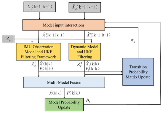
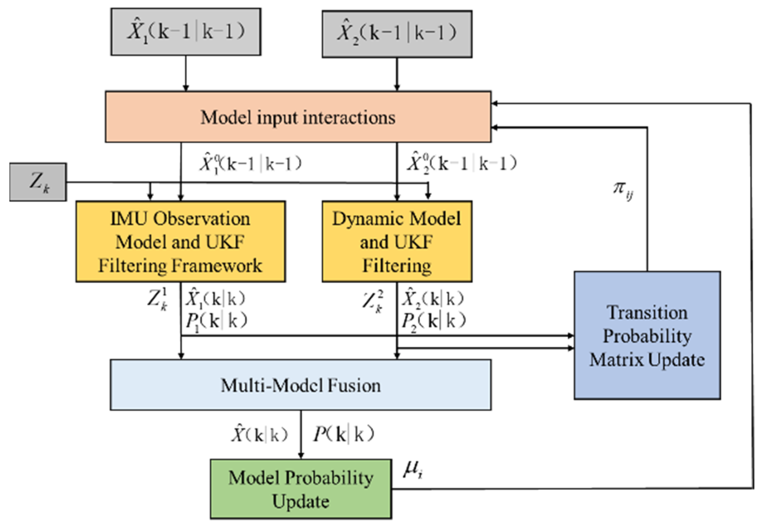
The overall TVIMM-UKF algorithm procedure is illustrated in Figure 2. The vehicle mass identified by the TVIMM-UKF algorithm is used as a real-time input for the brake force distribution optimization. According to the estimated mass, the braking control strategy dynamically updates the load-related constraints, including the ECE regulation boundaries and the ideal brake force distribution curve (I-curve).

Figure 2. Flowchart of the TVIMM-UKF algorithm.

3. Braking Control Strategy

This section presents the braking control strategy based on the estimated vehicle load. The estimated load is used to update the braking constraints, and an improved ABC algorithm is employed to optimize the front–rear braking force distribution. Based on the obtained braking force allocation, the regenerative braking and mechanical braking torques are further distributed to improve braking performance and energy recovery.

3.1. Ideal Brake Force Distribution

During braking, the force analysis of the vehicle indicates that the normal reactions exerted on the front and rear axles by the ground can be expressed as

$$\left\{\begin{array}{l}{F}_{zf}={\displaystyle \frac{mg}{L}}(b+z{h}_g)\\ F_{zr}={\displaystyle \frac{mg}{L}}(a-z{h}_g)\end{array}\right.$$

(24)

$$z={\displaystyle \frac{dv}{dt}}·{\displaystyle \frac{1}{g}}$$

(25)

where $F_{zf}$ and $F_{zr}$ denote the normal reaction forces on the front and rear tires, respectively; $L$ is the wheelbase; $a$ and $b$ are the distances from the vehicle’s center of gravity (CG) to the front and rear axles, respectively; $z$ is the braking intensity; and h_g is the height of the CG.

According to Equation (24), when the position of the vehicle’s CG changes, the normal forces on the front and rear axles fluctuate significantly. Assuming that the passengers are evenly distributed inside the bus, the relationship between the CG position and the vehicle load can be approximated as linear, as described in Equation (26). Therefore, the total load of the vehicle, identified through the load recognition model, can be further used to estimate the approximate position of the CG under the current loading condition.

$$\left\{\begin{array}{l}a={\displaystyle \frac{a_{Full}-a_{Empty}}{M_{Full}-M_{Empty}}}(M-M_{Empty})+a_{Empty}\\ b=L-a\\ h_g={\displaystyle \frac{h_{gFull}-h_{gEmpty}}{M_{Full}-M_{Empty}}}(M-M_{Empty})+h_{gEmpty}\end{array}\right.$$

(26)

Through dynamic analysis, it can be shown that under any given road adhesion coefficient, the condition for simultaneous wheel lock-up of the front and rear wheels can be expressed as

$$\left\{\begin{array}{l}{F}_{uf}+F_{ur}=\phi mg\\ F_{uf}=F_{xbf}=\phi F_{zf}\\ F_{ur}=F_{xbr}=\phi F_{zr}\end{array}\right.$$

(27)

where $F_{uf}$ and $F_{ur}$ denote the braking forces generated by the front and rear wheel brake actuators, respectively. By combining Equations (26) and (27) and eliminating the intermediate variable, Equation (28) is obtained.

$$F_{ur}={\displaystyle \frac{1}{2}}\left[{\displaystyle \frac{mg}{h_g}}\sqrt{b^2+{\displaystyle \frac{4h_{g}L}{mg}}{F}_{uf}}-\left({\displaystyle \frac{mgb}{h_g}}+2F_{uf}\right)\right]$$

(28)

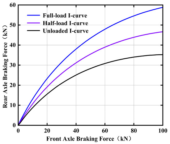
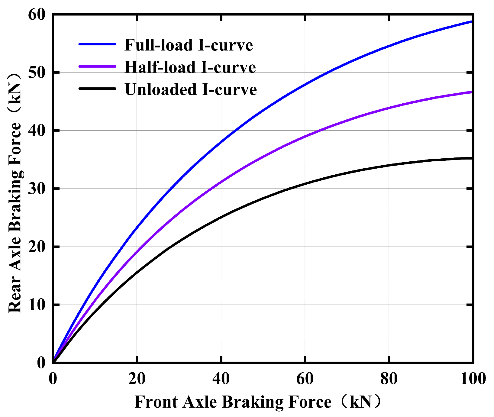
The theoretically derived Equation (28) describes the optimal distribution of braking force under the condition of simultaneous lock-up of the front and rear wheels. By substituting the technical parameters of the investigated vehicle into this mathematical model, as shown in Table 1. The I-curves of the vehicle under three representative loading conditions—fully loaded, half-loaded, and unloaded—are obtained, as shown in Figure 3. From the perspective of vehicle dynamics, the I-curve represents the ideal brake force distribution that allows the front and rear wheels to reach the adhesion limit simultaneously. When the vehicle load changes, the normal forces acting on the front and rear axles vary accordingly, which results in a shift in the feasible braking force distribution envelope defined by the ECE regulations.

Table 1. Main parameters of the vehicle.

Component	Description
Vehicle	Total mass: 15,500 kg; Wheelbase: 6150 mm Tire specification: 265/70R19.5 $\mathrm{Frontal} \mathrm{area}: 7.3 {\mathrm{m}}^2$; Drag coefficient: 0.6
IMU	$\mathrm{Accelerometer} \mathrm{measurement} \mathrm{range}: \pm 4 \mathrm{g}$ Shock resistance: 3000 g
Motor	Type: Permanent magnet synchronous motor Gear ratio: 19.22 Rated torque/speed/power: 325 N m/3250 rpm/ 110 kW Peak torque/speed/power: 650 N m/9000 rpm/ 220 kW
Battery	Type: Lithium iron phosphate Nominal voltage: 579.6 V; Rated capacity: 585 Ah Maximum discharge current: 426.24 A

Figure 3. I-curves under different load conditions.

3.2. Braking Force Constraints on Front and Rear Axles

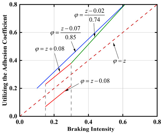
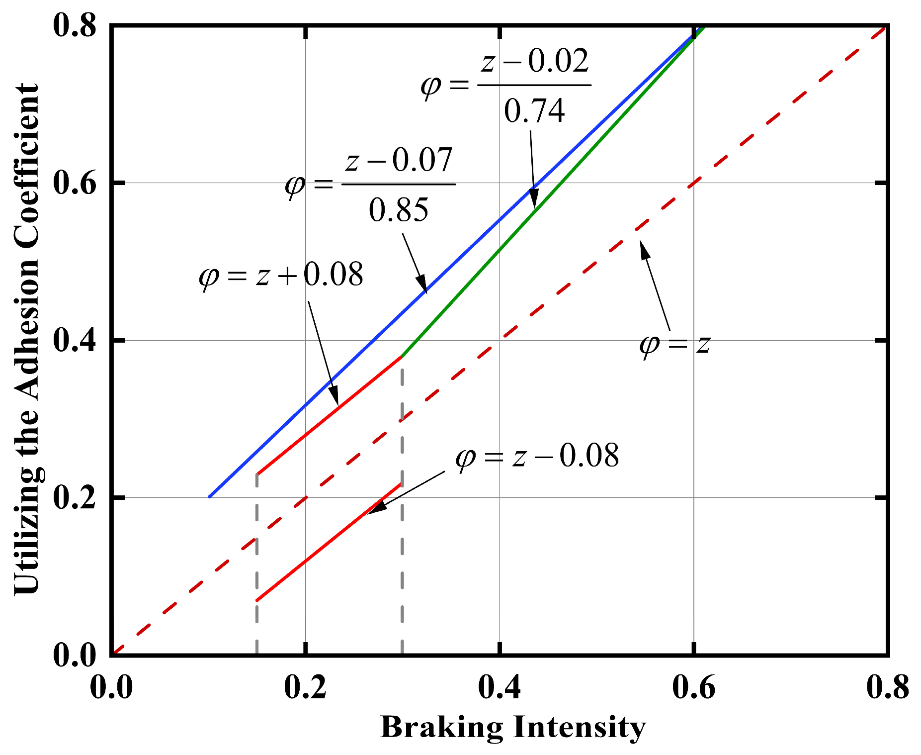
According to the ECE regulations, the braking forces on the front and rear axles are subject to specific constraints, as illustrated in Figure 4. For all M3-category vehicles, these constraints must be satisfied when the road adhesion coefficient lies within the range of 0.15 to 0.8.

Figure 4. Adhesion coefficient and brake intensity regulatory constraints.

Under regulatory constraints, the adhesion utilization coefficients of the front and rear axles, ${\phi }_f$ and ${\phi }_r$, can be expressed in terms of the braking intensity $z$:

$$\left\{\begin{array}{cc}z-0.08⩽{\phi }_r<{\phi }_f⩽z+0.08\hfill & 0.15⩽z⩽0.30\\ {\phi }_f⩽{\displaystyle \frac{z+0.07}{0.85}}\hfill & 0.10⩽z⩽0.61\\ {\phi }_r⩽{\displaystyle \frac{z+0.07}{0.85}}\hfill & 0.10⩽z⩽0.61\\ {\phi }_r⩽{\displaystyle \frac{z-0.02}{0.74}}\hfill & 0.30⩽z⩽0.61\end{array}\right.$$

(29)

The adhesion utilization coefficients of the front and rear axles, together with the braking force distribution coefficient $\beta$, can be expressed as

$$\left\{\begin{array}{l}{\phi }_f={\displaystyle \frac{F_{xbf}}{F_{zf}}}={\displaystyle \frac{\beta zL}{b+z{h}_g}}\\ {\phi }_r={\displaystyle \frac{F_{xbr}}{F_{zr}}}={\displaystyle \frac{(1-\beta )zL}{a-z{h}_g}}\end{array}\right.$$

(30)

$$\left\{\begin{array}{l}\beta ={\displaystyle \frac{F_{\mu f}}{F_{\mu }}}\\ F_{\mu }=F_{\mu f}+F_{\mu r}\\ {\displaystyle \frac{F_{\mu f}}{F_{\mu r}}}={\displaystyle \frac{\beta }{1-\beta }}\end{array}\right.$$

(31)

where $F_{xbf}$ and $F_{xbr}$ represent the ground-breaking forces acting on the front and rear axles, respectively.

By combining Equations (29)–(31), the admissible range of the braking force distribution coefficient $\beta$ under different braking intensities can be obtained.

$$\left\{\begin{array}{c}1-{\displaystyle \frac{\left(z+0.07\right)\left(a-z{h}_g\right)}{0.85zL}}⩽\beta ⩽{\displaystyle \frac{\left(z+0.07\right)\left(b+z{h}_g\right)}{0.85zL}}\hfill \\ 0.10⩽z⩽0.15\\ {\displaystyle \frac{b+z{h}_g}{L}}⩽\beta ⩽{\displaystyle \frac{\left(z+0.08\right)\left(b+z{h}_g\right)}{zL}}\hfill \\ 0.15⩽z⩽0.30\\ 1-{\displaystyle \frac{\left(z-0.02\right)\left(a-z{h}_g\right)}{0.74zL}}⩽\beta ⩽{\displaystyle \frac{\left(z+0.07\right)\left(b+z{h}_g\right)}{0.85zL}}\hfill \\ 0.30⩽z⩽0.61\end{array}\right.$$

(32)

Given that the regulations impose constraints when the road adhesion coefficient ranges from 0.15 to 0.8—corresponding to a braking intensity range of 0.1 to 0.61—the allowable distribution range of the braking forces between the front and rear axles can be calculated using Equation (32). Combining this with Equation (31) yields

$$\left\{\begin{array}{l}{F}_{uf}=\beta zmg\\ F_{ur}=zmg-F_{uf}\end{array}\right.$$

(33)

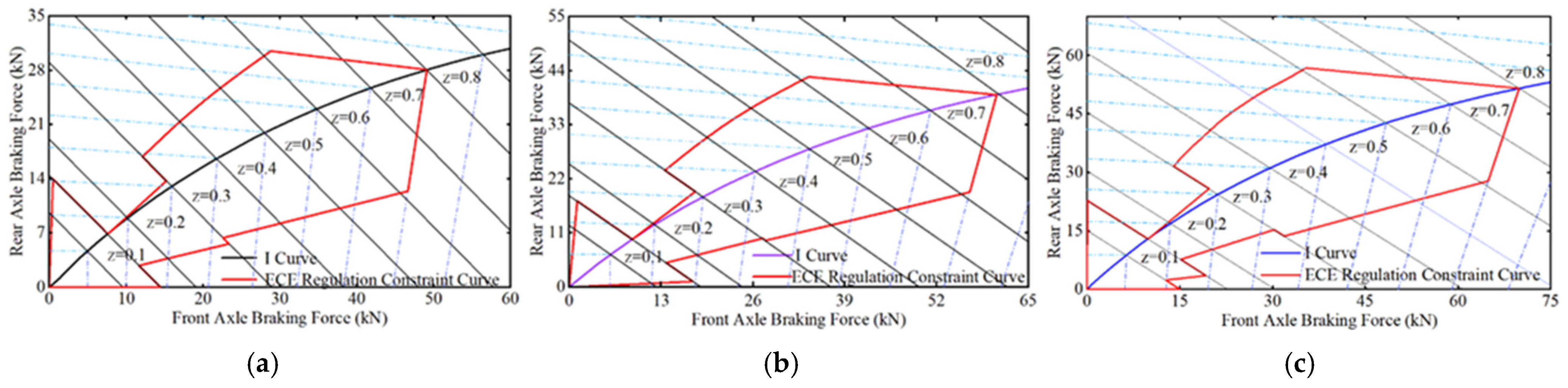
By substituting Equation (32) into Equation (33) and defining the range of braking intensity, the regulatory front–rear braking force distribution envelope of the target vehicle can be obtained. When the braking intensity lies between 0.1 and 0.61, the distribution curve satisfies the regulatory requirements. At a braking intensity of 0.61, the upper and lower boundary curves intersect the r- and f-lines at $\phi =0.8$. To ensure braking safety, when the braking intensity exceeds 0.61, the regulatory constraint curves continue along the r- and f-lines at $\phi =0.8$, intersecting with the I-curve. Conversely, when the braking intensity falls below 0.1, the upper and lower constraint lines coincide with the boundary, thereby imposing limitations.

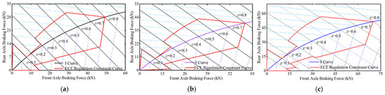
Figure 5a–c illustrate the regulatory constraint curves of the front and rear axle braking forces for the vehicle under three typical load conditions: unloaded, half-loaded, and fully loaded, respectively. The area between the two red lines represents the feasible region for front–rear braking force distribution that complies with regulations. As shown in the figures, with increasing vehicle load, the range of the regulatory constraint curves changes accordingly, imposing different requirements on the braking system’s control capabilities under varying load conditions.

Figure 5. Brake-force regulatory envelopes: (a) unladen; (b) half-load; (c) full-load.

3.3. Brake Force Distribution Using an Improved ABC Algorithm

The subject of this study is a pure electric rear-wheel-drive bus. To achieve coordinated braking control under varying load and braking intensity conditions, this section proposes an optimal front–rear brake force distribution scheme by integrating multiple constraints, including ECE regulations and I-curve considerations, while accounting for different load states and braking intensity demands. The ABC algorithm, a typical swarm intelligence optimization method, offers advantages such as few control parameters, a simple structure, and ease of implementation [25].

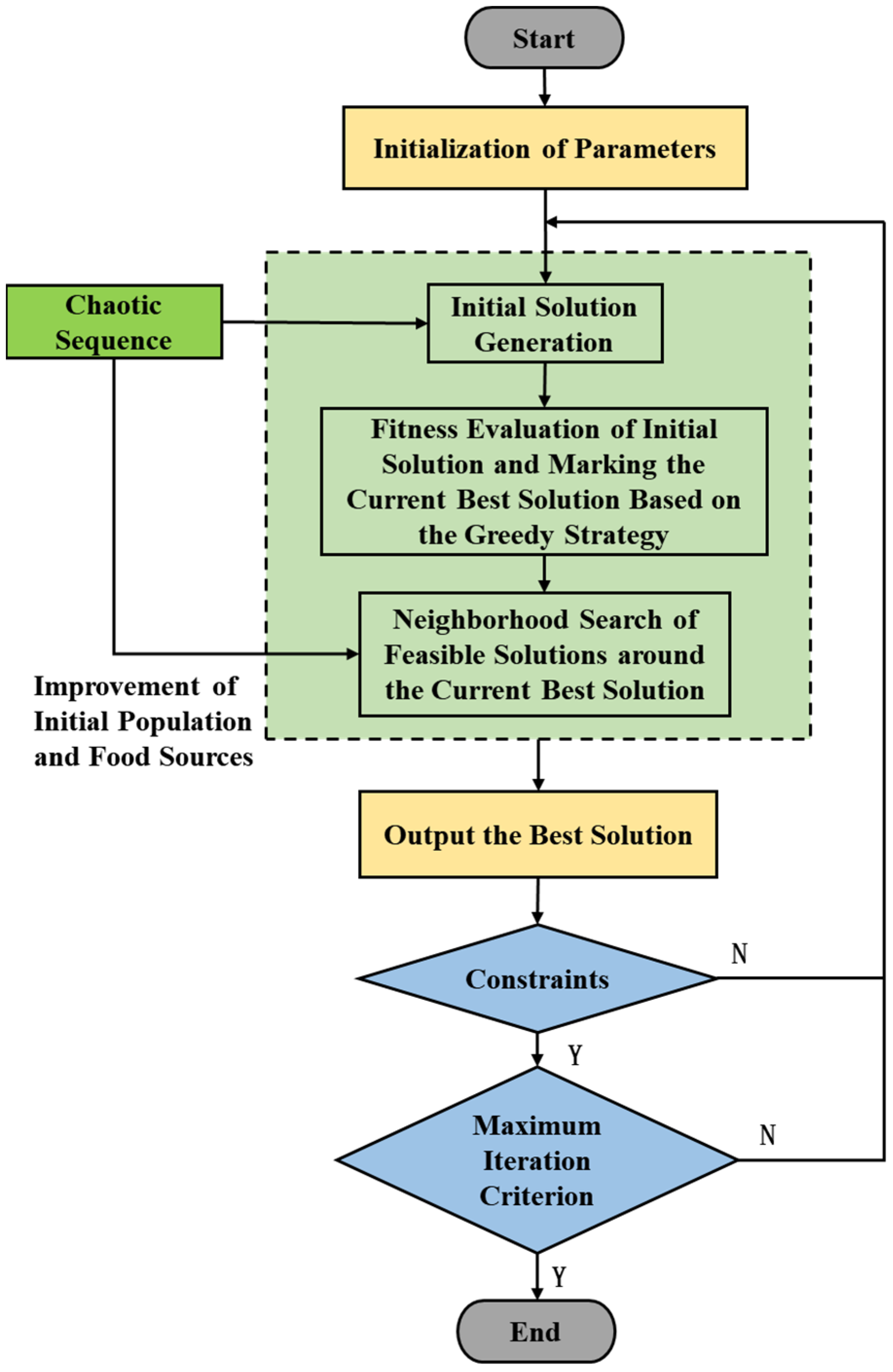
However, the standard ABC algorithm still has inherent limitations, including susceptibility to local optima and slow convergence. To address these issues, an improved ABC algorithm is proposed by embedding the Bernoulli chaotic map into the ABC algorithm to enhance population diversity and search exploration. The Bernoulli chaotic map is expressed as

$$x_{n+1}=\left\{\begin{array}{cc}{\displaystyle \frac{x_n}{1+\sigma }}\hfill & ,x_n\in (0,1-\sigma ]\\ {\displaystyle \frac{x_n-1+\sigma }{\sigma }}\hfill & ,x_n\in (1-\sigma ,1)\end{array}\right.$$

(34)

where $x_n$ denotes the chaotic sequence value at generation $n$, and $\sigma$ is the control parameter.

Before running the ABC algorithm, a chaotic sequence of a certain length is generated using the chaotic map. The improved initial population generation formula is given by

$$Z_k^j=Z_{\min }^j+x_{n+1}(Z_{max}^j-Z_{\min }^j)$$

(35)

where $Z_k^j$ is the $j$ dimension of the $k$ food source, $x_{n+1}$ is the value from the Bernoulli chaotic map, and $Z_{\min }^j$ and $Z_{max}^j$ denote the minimum and maximum values for the $j$ dimension.

By introducing the chaotic map into the food source update formula, the improved food source update is defined as

$${\nu }_k^j=X_k^j+{\phi }_k^j\left(X_k^j-X_i^j\right)+(x_{n+1}-0.5)$$

(36)

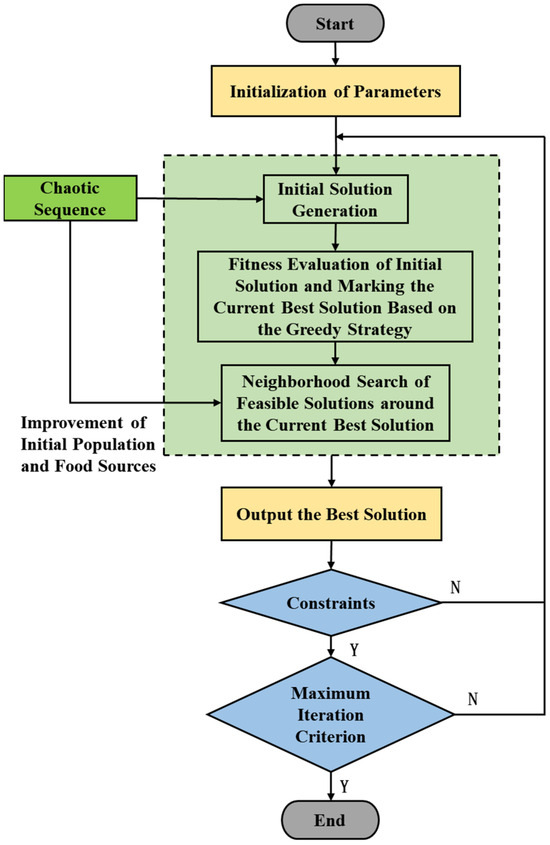
where ${\phi }_k^j$ is a random number within [−1, 1] and $X_i^j$ represents the initial neighborhood of the food source. All other steps follow the conventional ABC algorithm [26], and the workflow of the improved ABC algorithm is illustrated in Figure 6.

Figure 6. Flowchart of the improved ABC algorithm.

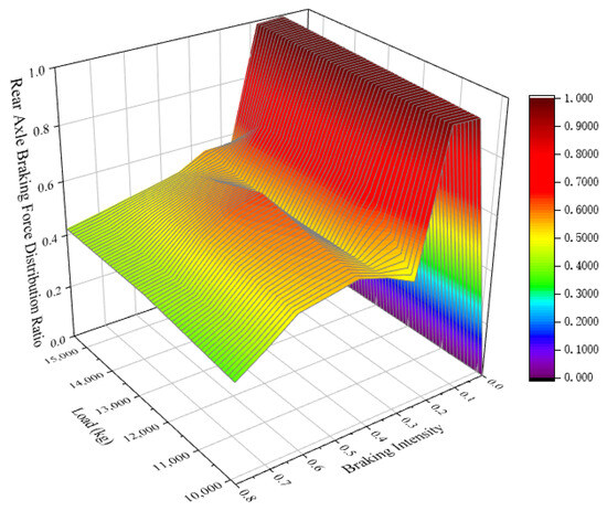
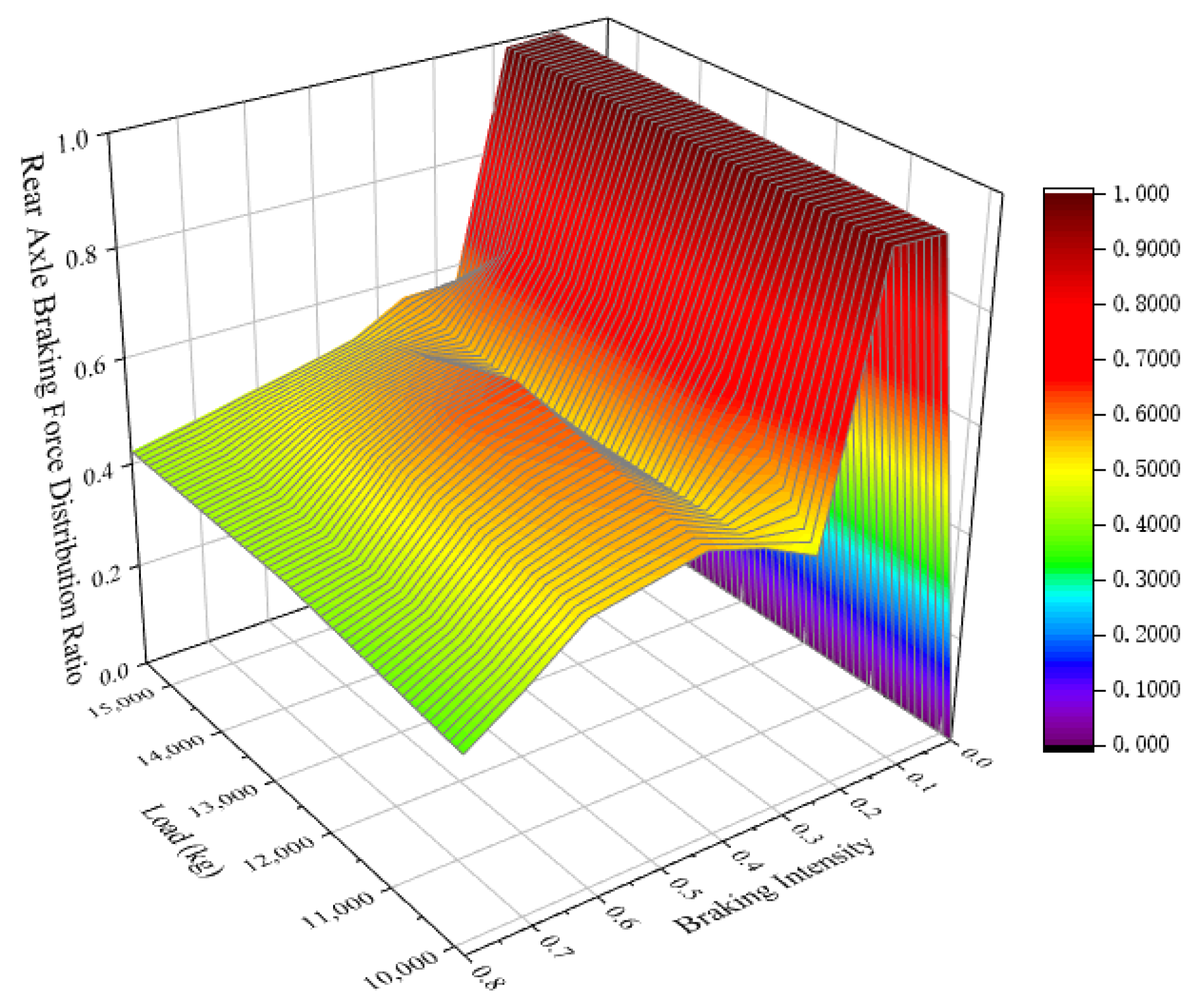
After determining the feasible region of the front–rear brake force distribution coefficients under the imposed constraints, the rear-axle brake force distribution coefficient is taken as the food source vector, and the improved ABC algorithm is then applied to optimize the brake force distribution parameters under different load and braking intensity conditions. The optimization results are shown in Figure 7.

Figure 7. Illustration of rear-axle brake force distribution coefficients under different load conditions.

3.4. Regenerative Braking Control Strategy Development

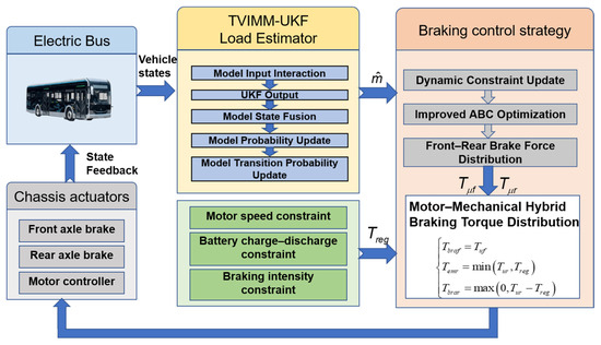
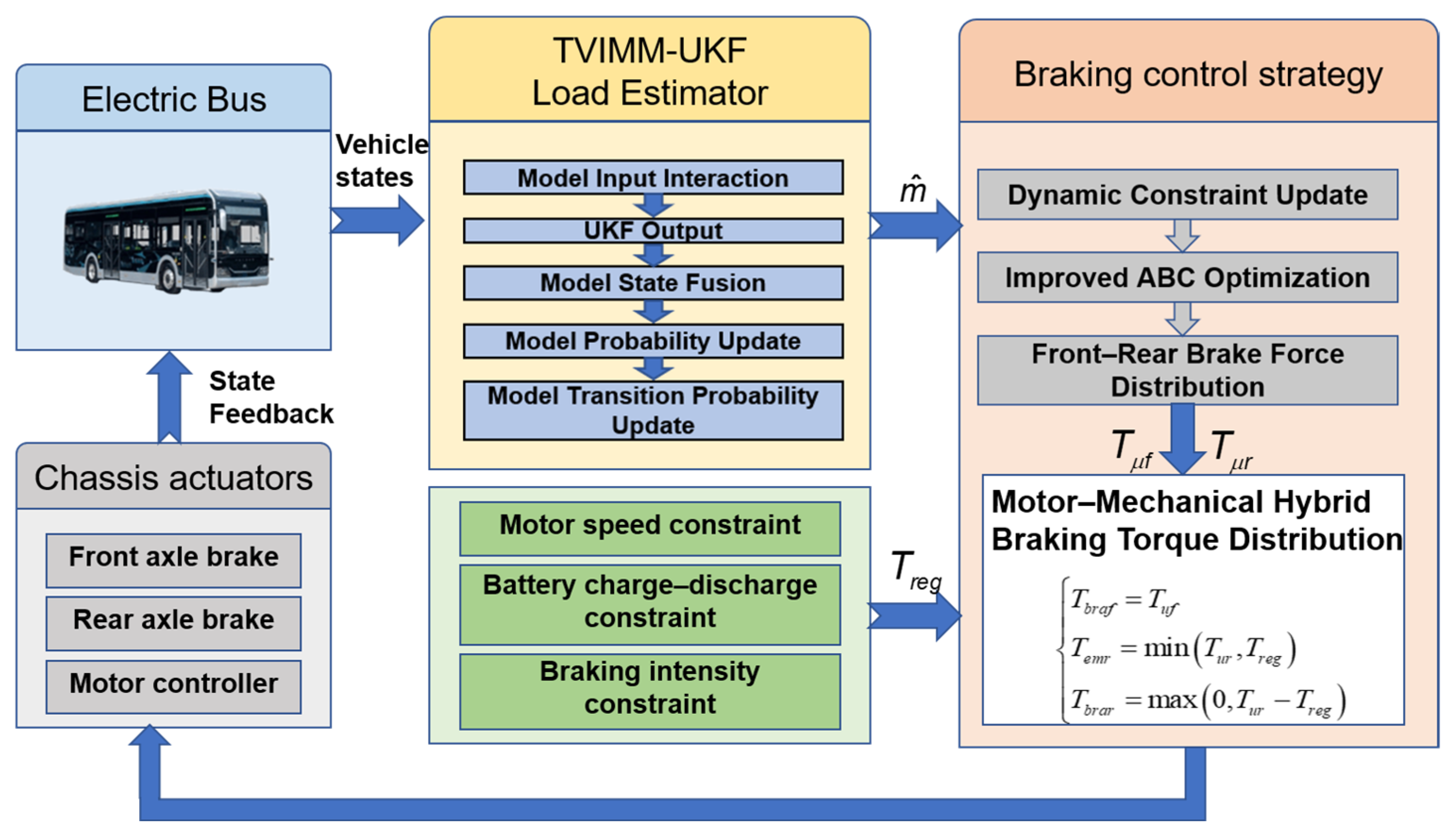
To optimize the coordinated control of braking performance and regenerative energy recovery, a load-estimation-based braking control strategy is developed. The overall control framework is illustrated in Figure 8. The vehicle load is identified online using a TVIMM-UKF-based algorithm. After the load estimation is completed, the identified load parameters together with the braking-intensity information are transmitted to the control module. The control module then computes the braking force distribution strategy appropriate for the current load condition and determines the optimal braking distribution curve based on vehicle parameters.

Figure 8. Overall framework of the control algorithm.

During practical implementation, a distribution principle that prioritizes motor regenerative braking with mechanical braking as compensation is adopted. Specifically, the maximum regenerative braking force achievable by the motor is first calculated according to the vehicle operating state, and any insufficient portion is compensated for by mechanical braking. The relationship of this distribution is expressed as follows:

$$\left\{\begin{array}{l}{T}_{braf}=T_{uf}\\ T_{emr}=\min \left(T_{ur},T_{reg}\right)\\ T_{brar}=\max \left(0,T_{ur}-T_{reg}\right)\end{array}\right.$$

(37)

where $T_{uf}$ and $T_{ur}$ denote the front and rear axle braking torques, $T_{emr}$ is the braking torque provided by the rear axle motor, and $T_{braf}$ and $T_{brar}$ are the mechanical friction braking torques of the front and rear axles, respectively. $T_{reg}$ represents the regenerative braking torque of the motor.

Subsequently, the calculated target brake force commands are sent to the chassis actuator controller to execute the complete braking control process.

A constraint model under high-adhesion road conditions is established, which describes the quantitative relationship between the maximum motor regenerative braking torque and its influencing factors, without considering wheel lock-up. The limitations on the maximum motor braking torque are described as follows.

(1)

Motor Speed Limitation

The maximum regenerative braking torque of the motor can be expressed as

$$T_{Reg(\max )}=\left\{\begin{array}{cc}0\hfill & 0<n⩽668.9\\ T_{\max }\hfill & 668.9<n⩽3250\\ {\displaystyle \frac{9550P_{\max }}{n}}\hfill & 3250<n\end{array}\right.$$

(38)

where $T_{\max }$ and $P_{\max }$ represent the maximum braking torque available at motor speed $n$ and the peak power, respectively. The critical speed of the motor in this study is 668.9 rpm, with a base speed of 3250 rpm. When the motor operates below the critical speed, regenerative braking is disabled, and the braking force is entirely provided by mechanical friction braking. As the vehicle speed increases, the proportion of braking force supplied by the motor can be appropriately raised to enhance energy recovery efficiency. Specifically, the motor critical speed of 668.9 rpm corresponds to a vehicle speed of 5.68 km/h, while the base speed of 3250 rpm corresponds to 27.62 km/h. A motor braking force influence coefficient, defined as a function of vehicle speed, is introduced to adjust the braking force. The formula for this influence coefficient is as follows:

$${\eta }_1=\left\{\begin{array}{cc}0& \nu ⩽5.68\hfill \\ 0.0456\nu -0.259& 5.68<\nu ⩽27.62\hfill \\ 1& 36⩽\nu \hfill \end{array}\right.$$

(39)

(2)

Battery Charge/Discharge Limitation

The SoC working range of the traction battery is 10–100%. To balance energy recovery efficiency and battery lifespan, the SoC range for regenerative braking is further limited to 15–85%. A corresponding correction coefficient is established to dynamically adjust the maximum regenerative braking torque of the motor, ensuring safe and effective energy recovery:

$${\eta }_2=\left\{\begin{array}{cc}0\hfill & 0<SOC⩽10\\ 0.2SOC-2\hfill & 10<SOC⩽15\\ 1\hfill & 15<SOC⩽85\\ -0.2SOC+18\hfill & 85<SOC⩽90\\ 0\hfill & 90<SOC⩽100\end{array}\right.$$

(40)

(3)

Braking Intensity Limitation

During emergency braking scenarios with braking intensity above 0.7, the system relies entirely on the mechanical friction braking system of the front and rear wheels to ensure driving safety. In this case, regenerative braking is disabled. A correction coefficient model is developed to adjust the calculation of the motor’s maximum regenerative braking torque:

$${\eta }_3=\left\{\begin{array}{cc}1& 0<z⩽0.65\\ -20z+14& 0.65<z⩽0.70\\ 0& 0.70<z\end{array}\right.$$

(41)

Based on the above limitations, the desired rear-axle braking torque and the regenerative braking torque are analyzed as follows.

(1)

Desired Rear-Axle Braking Torque

The deceleration demand during braking can be calculated from the current braking intensity:

$${\displaystyle \sum F=mgz}$$

(42)

According to the vehicle’s dynamic equilibrium during braking and its motion equations, the total braking force required for the electric vehicle is derived as

$$\begin{array}{l}{F}_b=F_{uf}+F_{ur}=F_{uf}+(F_{reg}+F_{brar})=\\ {\displaystyle \sum F-F_w-F_f-F_i}\end{array}$$

(43)

The desired rear-axle braking force is then expressed as

$$F_{ur}=(1-\beta )F_b$$

(44)

(2)

Maximum Motor Regenerative Braking Force

During braking, the maximum regenerative braking force the motor can provide is derived from its maximum braking torque:

$$F_{reg(\max )}={\displaystyle \frac{T_{reg(\max )}{i}_g{i}_0{\eta }_T}{r}}$$

(45)

(3)

Comparison of Desired Braking Force and Motor Capability

If the desired rear-axle braking force is less than or equal to the maximum regenerative braking force, the entire rear-axle braking demand is met by the motor to maximize energy recovery:

$$\left\{\begin{array}{l}{F}_{reg}=F_{ur}\\ F_{brar}=F_{ur}-F_{reg}=0\end{array}\right.$$

(46)

If the desired rear-axle braking force exceeds the motor’s maximum regenerative braking force, the motor provides its maximum available regenerative braking, and the remaining torque is supplied by the rear-axle mechanical friction brakes:

$$\left\{\begin{array}{l}{F}_{reg}=F_{reg(\max )}\\ F_{brar}=F_{ur}-F_{reg}\end{array}\right.$$

(47)

Thus, the maximum regenerative braking torque the motor can provide is

$$T_{reg}=T_{reg(\max )}·{\eta }_1·{\eta }_2·{\eta }_3$$

(48)

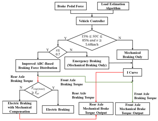
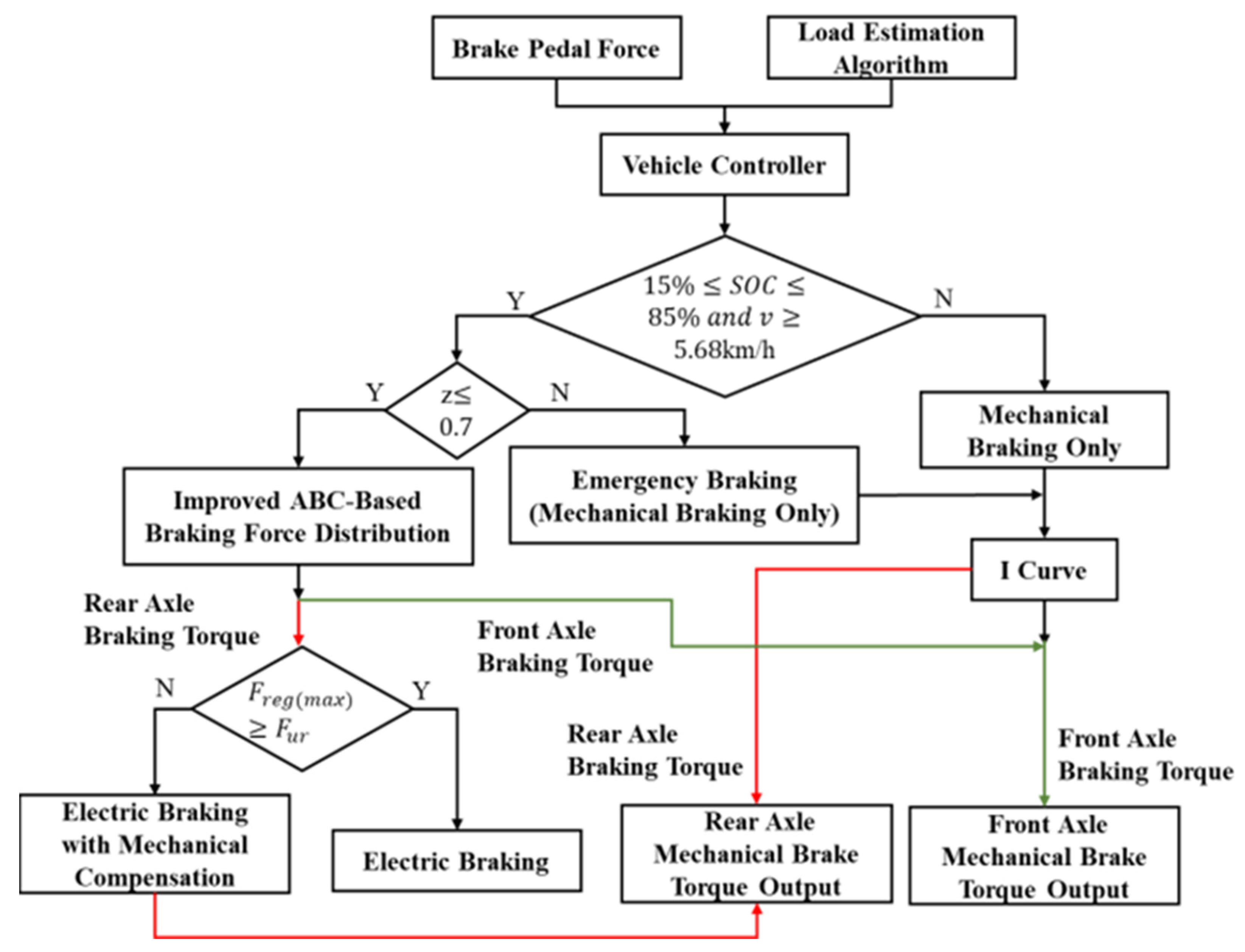
The workflow of the proposed regenerative braking control strategy is illustrated in Figure 9. In the flowchart, the red line denotes the rear axle braking torque path, whereas the green line denotes the front axle braking torque path.

Figure 9. Flowchart of the regenerative braking control strategy.

Specifically, the vehicle control unit (VCU) receives the brake pedal signal to determine the driver’s braking demand while simultaneously obtaining the current vehicle load state. The system then evaluates whether the battery SoC and vehicle speed satisfy the conditions for regenerative braking. If the SoC is below 15% or above 85%, or the vehicle speed is less than 5.68 km/h, regenerative braking is not allowed, and the front–rear axle braking forces are distributed according to the I-curve corresponding to the current load state.

If the regenerative braking constraints are satisfied and the braking intensity $z\le 0.7$, the front–rear braking forces are allocated based on the pre-defined distribution strategy, taking into account the brake pedal signal, load parameters, and vehicle operating conditions. When the motor braking torque is sufficient to meet the desired rear-axle braking force, the braking force is entirely provided by the motor; otherwise, the mechanical braking system supplements the remaining torque. For emergency braking scenarios where $z>0.7$, mechanical braking is applied according to the I-curve without regenerative braking.

4. Simulation Validation

A full-vehicle model of a pure electric rear-wheel-drive city bus was developed using AVL Cruise, based on the specific parameters provided by the project partner. The braking control strategy was implemented on the MATLAB (R2024a)/Simulink platform, forming an integrated co-simulation framework. The main vehicle parameters are summarized in Table 1.

4.1. Validation of Vehicle Load Estimation Using the TVIMM-UKF Algorithm

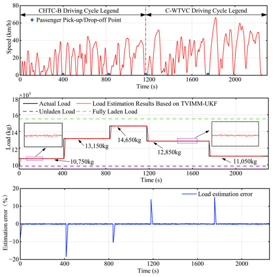
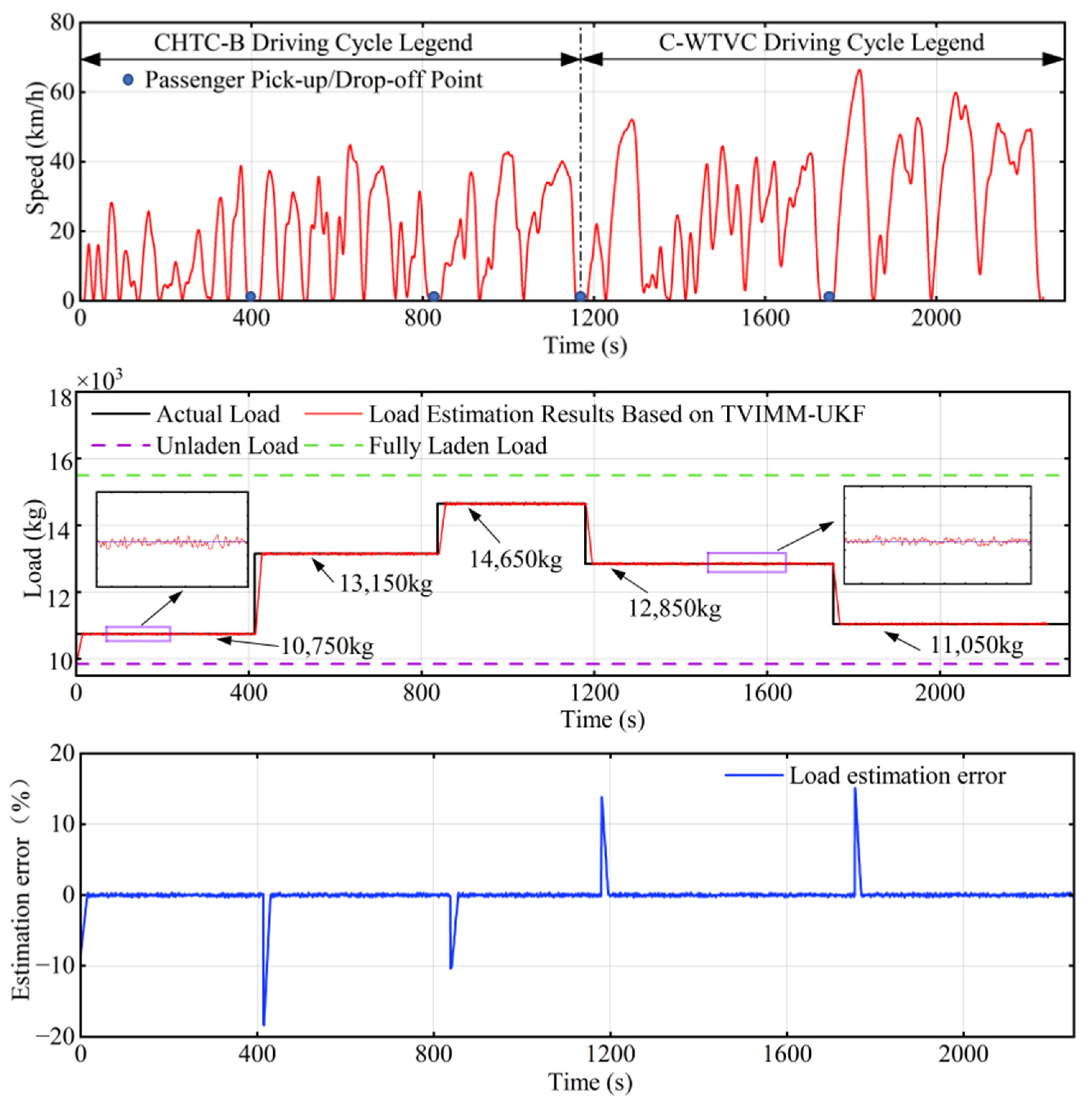
To evaluate the robustness of the proposed algorithm under dynamically varying operating conditions, a composite driving cycle with a total duration of 2250 s was constructed by integrating the CHTC-B and C-WTVC driving cycles. This composite cycle effectively represents the typical operational characteristics of urban buses.

During the simulation, dynamic load variations were modeled by introducing passenger boarding and alighting events during vehicle idle periods. The initial vehicle mass was set to 10,750 kg, and several load change events were introduced during the driving cycle to simulate passenger flow at bus stops. Specifically, the vehicle mass increased to 13,150 kg at 415 s, further increased to 14,650 kg at 840 s, then decreased to 12,850 kg at 1180 s, and finally reduced to 11,050 kg at 1750 s. These settings created a time-varying load scenario consisting of five distinct loading stages for offline simulation analysis. The corresponding results are presented in Figure 10.

Figure 10. Load estimation results of the TVIMM-UKF algorithm.

The simulation results indicate that the TVIMM-UKF algorithm can respond rapidly to dynamic input variations, completing the update of the vehicle’s load estimation within a short period. The algorithm demonstrates good real-time performance and tracking capability. In terms of estimation accuracy, the maximum absolute error remains consistently low. Although minor fluctuations occur during load transition phases, the estimated values quickly converge to the actual load. Across the entire driving cycle, the relative mean error of the estimation is 3.68%. These results demonstrate that the proposed algorithm maintains robust and accurate performance under complex and variable loading conditions, thereby validating its effectiveness for vehicle load estimation in dynamic operational environments.

4.2. Validation of Regenerative Braking Performance

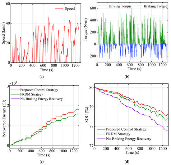
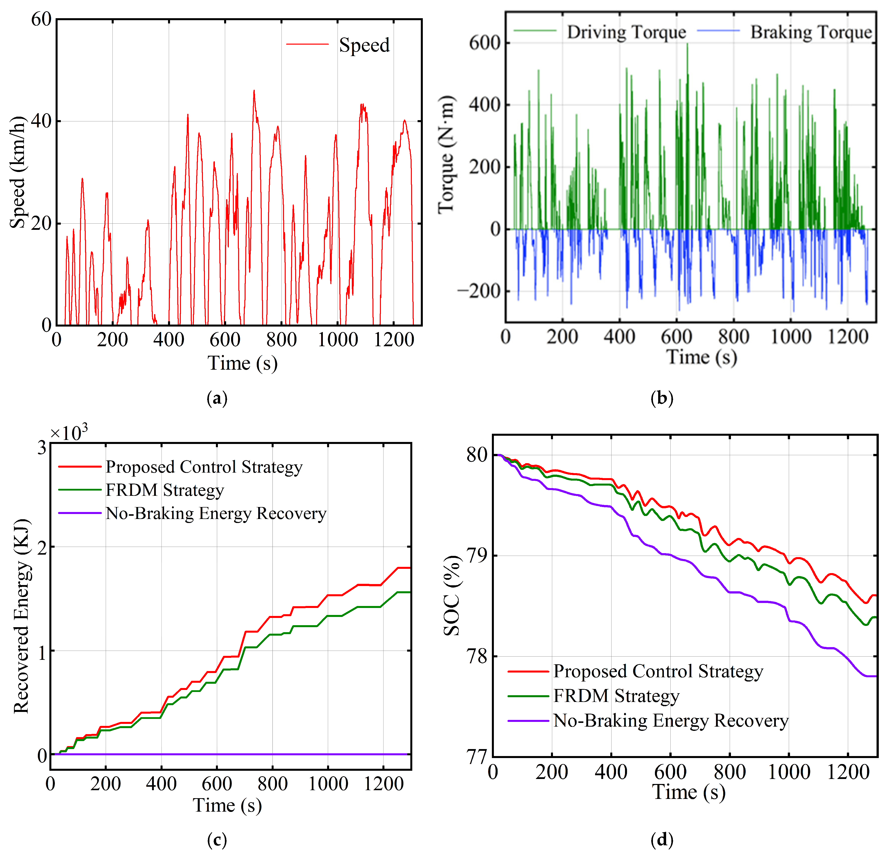
To verify the braking energy recovery capability of the proposed control strategy, evaluations were conducted under the CHTC-B driving cycle, which has a total duration of 1310 s, a maximum vehicle speed of 45.6 km/h, and a single-cycle distance of 5.49 km. During the cycle, three different vehicle load conditions were applied: near full load (15,010 kg), near empty load (10,210 kg), and near half load (12,370 kg), representing peak-hour full-load operation, light-load operation after passenger alighting, and partial passenger load conditions, respectively. The experimental results are presented in Figure 11 and Table 2.

Figure 11. Results under the CHTC-B driving cycle: (a) vehicle speed; (b) driving and braking torques; (c) comparison of energy recovery capability; (d) comparison of SoC consumption.

Table 2. Results under the CHTC-B driving cycle.

	No-Braking Energy Recovery	FRDM Strategy	Proposed Control Strategy
Total regenerative braking energy (kJ)	0	1573.2	1807.6
SoC consumption (%)	2.2	1.61	1.39

The results demonstrate that the proposed load-estimation-based braking control strategy achieves superior energy optimization under identical driving conditions. Without any energy recovery strategy, the vehicle’s SoC decreased by 2.2%, and no braking energy was recovered. With the FRDM method, the recovered braking energy increased to 1573.2 kJ, and SoC consumption was reduced to 1.61%. In contrast, the proposed strategy dynamically identifies the vehicle load and optimizes the braking force distribution, achieving a recovered braking energy of 1807.6 kJ and further reducing SoC to 1.39%, representing a 12.9% improvement in braking energy recovery compared with the FRDM method.

Considering that the effectiveness of regenerative braking energy recovery is highly sensitive to driving cycles, significant differences exist in vehicle speed distribution and braking frequency under different operating conditions. Validation under a single driving cycle is therefore insufficient to fully reflect the universality of the proposed strategy in bus operation scenarios. Accordingly, in addition to the typical comprehensive bus driving cycle CHTC-B, the urban driving cycle C-WTVC with more pronounced stop-and-go characteristics is further selected to evaluate the energy recovery performance of the proposed regenerative braking control strategy under different load conditions.

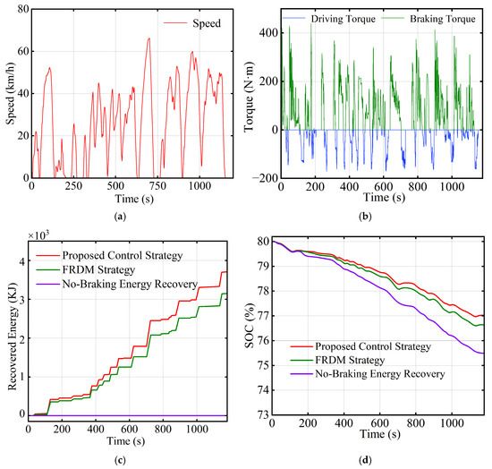
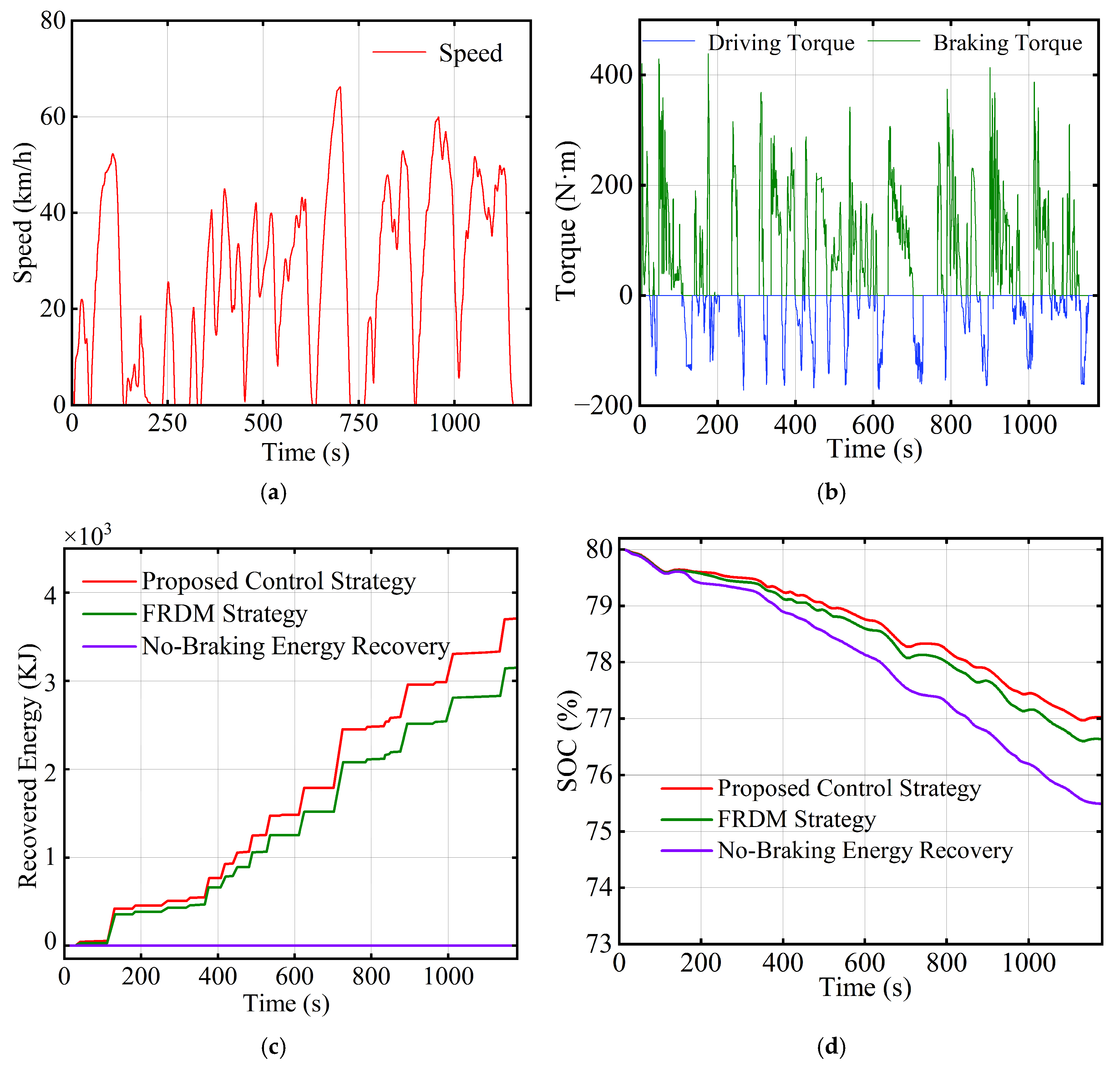
The total duration of the C-WTVC driving cycle is 1800 s, with a maximum vehicle speed of 87.8 km/h. Considering that the maximum speed of the research object in this study is 69 km/h, which cannot satisfy the high-speed operation requirements of the original cycle, only the urban and suburban segments are extracted for simulation. The resulting truncated cycle has a total duration of 1310 s and a maximum speed of 45.6 km/h. The load conditions are set identically to those in the CHTC-B cycle. The simulation results are presented in Figure 12 and Table 3.

Figure 12. Results under the C-WTVC driving cycle: (a) vehicle speed; (b) driving and braking torques; (c) comparison of energy recovery capability; (d) comparison of SoC consumption.

Table 3. Results under the C-WTVC driving cycle.

	No-Braking Energy Recovery	FRDM Strategy	Proposed Control Strategy
Total regenerative braking energy (kJ)	0	3142.2	3713.6
SoC consumption (%)	4.5	3.38	2.98

Under the C-WTVC driving cycle, the simulation results further verify the effectiveness of the proposed strategy. Without any regenerative braking strategy, no braking energy is recovered and the battery SoC decreases by 4.5%. When the FRDM strategy is applied, the recovered braking energy increases to 3142.2 kJ and the SoC consumption is reduced to 3.38%. By contrast, the proposed strategy dynamically identifies the vehicle load and optimizes the brake force distribution, achieving a higher recovered braking energy of 3713.6 kJ while further reducing the SoC consumption to 2.98%. Compared with the FRDM strategy, the proposed method improves braking energy recovery by 18.2% under the C-WTVC driving cycle. Moreover, due to the frequent stop-and-go behavior and intensive braking events of the C-WTVC cycle, the proposed strategy exhibits a more pronounced advantage in energy recovery, demonstrating its good applicability to typical urban bus operating conditions.

By comparing the results obtained under the CHTC-B and C-WTVC driving cycles, it can be observed that the proposed strategy consistently outperforms the benchmark FRDM method under different operating conditions. Although the absolute amount of recovered braking energy varies with driving cycle characteristics, the proposed strategy maintains a stable advantage in both energy recovery and SoC reduction across the two cycles. It demonstrates that the proposed strategy exhibits strong adaptability and robustness to different braking distribution characteristics and speed profiles, validating the engineering potential and value of the proposed dynamic strategy in extending the driving range of electric buses.

5. Conclusions

To enhance the adaptive capability of the braking system and improve braking energy recovery performance under varying vehicle load conditions, this study proposes a braking control strategy for pure electric buses operating under time-varying loads. The main conclusions of this study are summarized as follows.

Vehicle Load estimation: To address the challenge that a single model cannot fully capture dynamic changes in the target state, a TVIMM-UKF-based load estimation method was developed. Simulation results indicate that this method exhibits good estimation accuracy and robustness under various load-changing scenarios, with a relative mean error of 3.68% across the entire cycle, providing a reliable foundation for subsequent braking control research.

Braking Force Distribution and Regenerative Braking Control: An improved ABC algorithm was proposed to achieve optimal braking force distribution for different loads under varying braking intensities. Based on this, a regenerative braking control strategy was developed by considering motor characteristics and system operational constraints. Simulation results based on the two typical bus driving cycles, CHTC-B and C-WTVC, demonstrate that the proposed load-estimation-based regenerative braking control strategy can effectively improve braking energy recovery performance under different load conditions. Compared with the FRDM method, the proposed strategy increases braking energy recovery by 12.9% under the CHTC-B cycle, and the improvement further rises to 18.2% under the more frequent-braking C-WTVC cycle, validating that the strategy possesses good adaptability and robustness across different driving conditions.

References

- Jia, C.; Liu, W.; He, H.; Chau, K.T. Superior energy management for fuel cell vehicles guided by improved DDPG algorithm: Integrating driving intention speed prediction and health-aware control. Appl. Energy 2025, 394, 126195. [Google Scholar] [CrossRef] [Scilit]
- Li, K.; Zhou, J.; Jia, C.; Yi, F.; Zhang, C. Energy sources durability energy management for fuel cell hybrid electric bus based on deep reinforcement learning considering future terrain information. Int. J. Hydrogen Energy 2024, 52, 821–833. [Google Scholar] [CrossRef] [Scilit]
- Eliyan, A.F.; Haouari, M.; Sleiti, A. Decarbonizing Public Transportation: A Multi-Criteria Comparative Analysis of Battery Electric Buses and Fuel Cell Electric Buses. Sustainability 2024, 16, 9354. [Google Scholar] [CrossRef] [Scilit]
- Ekici, Y.E.; Karadağ, T.; Akdağ, O. Redefining urban mobility: Real-world regenerative braking optimization via bio-inspired AI for electric buses energy efficiency. Energy 2025, 338, 138854. [Google Scholar] [CrossRef] [Scilit]
- Cai, W.; Liu, C. Long Downhill Braking and Energy Recovery of Pure Electric Commercial Vehicles. World Electr. Veh. J. 2024, 15, 51. [Google Scholar] [CrossRef] [Scilit]
- Wu, T.; Wang, F.; Ye, P. Regenerative braking strategy of dual-motor EV considering energy recovery and brake stability. World Electr. Veh. J. 2023, 14, 19. [Google Scholar] [CrossRef] [Scilit]
- Girovský, P.; Žilková, J.; Kaňuch, J. Optimization of vehicle braking distance using a fuzzy controller. Energies 2020, 13, 3022. [Google Scholar] [CrossRef] [Scilit]
- Mirzaei, M.; Vali, A.R.; Allahverdizadeh, F.; Behnamgol, V. Fixed-time dynamic control allocation for the distribution of braking forces in a vehicle ESC system. Nonlinear Dyn. 2024, 112, 22009–22037. [Google Scholar] [CrossRef] [Scilit]
- He, Q.; Yang, Y.; Luo, C.; Zhai, J.; Luo, R.; Fu, C. Energy recovery strategy optimization of dual-motor drive electric vehicle based on braking safety and efficient recovery. Energy 2022, 248, 123543. [Google Scholar] [CrossRef] [Scilit]
- Wang, J.C. Hierarchical braking accurate control of electrohydraulic composite braking system for electric vehicles. ISA Trans. 2025, 158, 594–608. [Google Scholar] [CrossRef] [Scilit] [PubMed]
- Liu, J.; Hua, Y.; Zhou, Z.; Pan, Y. Research on Braking Force Distribution Strategy for Race Cars Based on PID Algorithm. World Electr. Veh. J. 2025, 16, 653. [Google Scholar] [CrossRef] [Scilit]
- Li, H.; Jin, L.; Li, J.; Xiao, F.; Wang, Z.; Zhang, G. Braking Force Coordination Control for In-Wheel Motor Drive Electric Vehicles with Electro-Hydraulic Composite Braking System. Vehicles 2025, 7, 119. [Google Scholar] [CrossRef] [Scilit]
- Wang, Y.; Zhou, L.; Chu, L.; Zhao, D.; Guo, Z.; Jiang, Z. A Multi-Source Braking Force Control Method for Electric Vehicles Considering Energy Economy. Energies 2024, 17, 2032. [Google Scholar] [CrossRef] [Scilit]
- Liu, J.; Bu, L.; Fu, B.; Zheng, J.; Wang, G.; He, L.; Hu, Y. Research on adaptive distribution control strategy of braking force for pure electric vehicles. Processes 2023, 11, 1152. [Google Scholar] [CrossRef] [Scilit]
- Faghihian, H.; Sargolzaei, A. A novel energy-efficient automated regenerative braking system. Appl. Energy 2025, 390, 125746. [Google Scholar] [CrossRef] [Scilit]
- Li, C.; Zhang, L.; Lian, S.; Liu, M. Research on regenerative braking control of electric vehicles based on game theory optimization. Sci. Prog. 2024, 107, 00368504241247404. [Google Scholar] [CrossRef] [Scilit]
- Cai, L.; Yan, P.; Yang, X.; Yang, L.; Liu, Y.; Huang, G.; Liu, S.; Fan, J. Braking Energy Recovery Control Strategy Based on Instantaneous Response and Dynamic Weight Optimization. Machines 2025, 14, 10. [Google Scholar] [CrossRef] [Scilit]
- Chengqun, Q.; Wan, X.; Wang, N.; Cao, S.; Ji, X.; Wu, K.; Hu, Y.; Meng, M. A novel regenerative braking energy recuperation system for electric vehicles based on driving style. Energy 2023, 283, 129055. [Google Scholar] [CrossRef] [Scilit]
- Zhou, X.; Wu, G.; Wang, C.; Zhang, R.; Shi, S.; Zhao, W. Cooperative optimization of energy recovery and braking feel based on vehicle speed prediction under downshifting conditions. Energy 2024, 301, 131699. [Google Scholar] [CrossRef] [Scilit]
- Jia, C.; Liu, W.; Chau, K.T.; He, H.; Zhou, J.; Niu, S. Passenger-aware reinforcement learning for efficient and robust energy management of fuel cell buses. eTransportation 2026, 27, 100537. [Google Scholar] [CrossRef] [Scilit]
- Ritter, A.; Widmer, F.; Vetterli, B.; Onder, C.H. Optimization-based online estimation of vehicle mass and road grade: Theoretical analysis and experimental validation. Mechatronics 2021, 80, 102663. [Google Scholar] [CrossRef] [Scilit]
- Feng, J.; Qin, D.; Liu, Y.; You, Y. Real-time estimation of road slope based on multiple models and multiple data fusion. Measurement 2021, 181, 109609. [Google Scholar] [CrossRef] [Scilit]
- Gao, J.; Zhang, Q.; Sun, H.; Wang, W. A multi-sensor interacted vehicle-tracking algorithm with time-varying observation error. Remote Sens. 2022, 14, 2176. [Google Scholar] [CrossRef] [Scilit]
- Yuen, K.V.; Liu, Y.S.; Yan, W.J. Estimation of time-varying noise parameters for unscented Kalman filter. Mech. Syst. Signal Process. 2022, 180, 109439. [Google Scholar] [CrossRef] [Scilit]
- Yu, H.; Kang, Y.; Kang, L.; Zeng, J. Bi-preference linkage-driven artificial bee colony algorithm with multi-operator fusion. Complex Intell. Syst. 2023, 9, 6729–6751. [Google Scholar] [CrossRef]
- Jiang, Y.; Qian, H.; Chu, Y.; Liu, J.; Jiang, Z.; Dong, F.; Jia, L. Convergence analysis of ABC algorithm based on difference model. Appl. Soft Comput. 2023, 146, 110627. [Google Scholar] [CrossRef] [Scilit]
Disclaimer/Publisher’s Note: The statements, opinions and data contained in all publications are solely those of the individual author(s) and contributor(s) and not of MDPI and/or the editor(s). MDPI and/or the editor(s) disclaim responsibility for any injury to people or property resulting from any ideas, methods, instructions or products referred to in the content. |
© 2026 by the authors. Licensee MDPI, Basel, Switzerland. This article is an open access article distributed under the terms and conditions of the Creative Commons Attribution (CC BY) license.