On Mechanical and Chaotic Problem Modeling and Numerical Simulation Using Electric Networks

Abstract

After reviewing the use of electrical circuit elements to model dynamic processes or the operation of devices or equipment, both in real laboratory implementations and through ideal circuits implemented in simulation software, a network model design protocol is proposed. This approach, following the basic rules of circuit theory, makes use of controlled generators to implement any type of nonlinearity contained in the governing equations. Such a protocol constitutes an interesting educational tool that makes it possible for nonexpert students in mathematics to design and numerically simulate complex physical processes. Three applications to mechanical and chaotic problems are presented to illustrate the versatility of the proposed protocol.

1. Introduction

The simulation of physical or engineering processes by means of models designed in the laboratory is a very old resource that allows predicting both the steady state solution and the time evolution of these systems in a simpler, more economical, and often reliable way. For the elaboration of these models, based on the mathematical equivalence of the physical equations of the real process and the equations of the laboratory prototype, different techniques were used, such as the use of membranes (soap film analogy), chemical solutions (electrolytic tank), graph paper (analog field plotter), construction of electrical circuits, and reduced models based on scale factors. Thus, and sticking to the subject of electrical analogy, based on the laws of electric circuits, we should mention the first attempts to successfully simulate processes governed by Laplace’s equation through the construction of an electrolytic tank [1], or a century later with the use of graphite paper (analog field plotter [2]). More recently, Arvinti et al. [3] implemented a laboratory electrical model to solve the Laplace equation in the whole domain, approaching the solutions using Lagrange polynomials. During the decades between 1940 and 1970, large analog equipment consisting of resistors and capacitors were developed that allowed the simulation of heat and mass flow processes both linear, with the ‘heat and mass analyzer’ of Paschkis and Heisler [4], and nonlinear, by means of the ‘differential analyzer’ of Karplus and Soroka [5]. After the development of computers, these physical models were replaced by numerical computational techniques that directly address the solution to governing equations using a variety of precise methods, such as finite elements, finite differences, and variational techniques. Table 1 lists the different models developed in historical order with their applications.

Table 1. History of laboratory and computer-developed models.

Authors	Year	Model	Problem
Kirchhoff [1]	1845	Electrolytic tank	Electrical currents on conductive surfaces
Paschkis and Heisler [4]	1944	Resistors and capacitors (laboratory)	Heat transfer
Kayan [2]	1945	Graphite paper	Heat fluxes
Karplus and Soroka [5]	1959	Resistors and capacitors (laboratory)	Heat and mass transfer
Horno et al. [6]	1990	Network method (Pspice)	Transport through membranes
López-García et al. [7]	1996	Network method (Pspice)	Colloidal systems
López-García et al. [8]	1999	Network method (Pspice)	Thermodynamic colloidal systems
Chen et al. [9]	2006	Pspice	Heat transfer
Meca et al. [10]	2007	Network method (Pspice)	Flow and salt transport
Bég et al. [11]	2009	Network method (Pspice)	Magnetohydrodynamic systems
Serna et al. [12]	2014	Network method (Pspice)	Lid cavity problem
Cánovas et al. [13]	2015	Network method (Pspice)	Flow and heat transport
Cánovas et al. [14]	2017	Network method (Pspice)	Density driven flow
García-Ros et al. [15]	2017	Network method (Pspice)	Soil consolidation systems
Rossi et al. [16]	2018	Network models	Semiconductors
Akram et al. [17]	2019	Network models (LTspice)	Thermal heating
Yaqoob and Obed [18]	2019	Semiconductor networks (Proteus)	Photovoltaic
Arvinti et al. [3]	2020	Electrical resistors (laboratory)	Electrostatic
Garratón et al. [19]	2023	Network models (Pspice)	Delay differential equations
Lineykin et al. [20]	2023	Electric analogy	Thermoelectric harvest equipment
Sánchez-Pérez et al. [21]	2023	Network method (Ngspice)	Burgers-Huxley problems

Thanks to the evolution of digital computers, the ideal zero-tolerance electrical models that replaced the nonzero tolerance models—abandoned in the 1960s—have, in recent decades, come back into use as a very useful simulation tool [9,16,20]. Nowadays, the protocol of elaboration of these models and their numerical simulation is called the network method [7,19,21,22]. We can say that the modeling technique based on electrical analogy has been recycled so that the real circuits developed in the laboratory are now implemented by ideal circuits, equivalent to the previous ones, that are numerically solved in the computer by means of a suitable circuit simulation program, such as Pspice [23], Proteus [18], LTspice [17], and others. The equivalence between these ideal circuits and the physical processes to be simulated is ensured by the fact that both are formally ruled by the same governing equations although with different dependent variables. The reliability of the results, which has been verified by the solution of several benchmark problems [10,13], is ensured by the powerful computational algorithms implemented in these programs that allow the quasi-exact solution of the circuit when the only independent variable is time–ordinary differential equations. Such is the case of the dynamic problems presented in this work.

Advantages of models based on electrical analogy include (i) the circuits containing ideal electrical devices (zero manufacturing tolerance) and ideal electric contact between them, which does not induce errors in the solutions for this reason; (ii) the circuit resolution programs containing in their libraries a wide range of electrical devices and programming sentences, which allows for implementing any type of physical problem in the models, particularly the so-called controlled generators, which allow for implementing any nonlinear or coupled term that is part of the governing equations; (iii) the computer algorithms developed in these programs being perhaps the most up-to-date, optimized, and computationally powerful, which results in the reliability of the numerical solutions and the reduction of computation time [24]; and (iv) the programming rules for preparing the text files of the models being relatively few and established on the basic theory of electric circuits, i.e., on the constitutive laws of their elements and on the theorems of uniqueness of the electric potential and conservation of electric charge (Kirchhoff’s theorems) [22]. In fact, the researcher only has to worry about the correct design of the network model—or equivalent circuit—which has to collect the boundary and initial conditions of the problem, forgetting about the algorithms for numerical computation.

Numerous researchers have used this analogy by applying it to complex problems in different fields of physics and engineering, as shown in Table 1. Horno et al. [22] apply it to charge transfer processes in membranes, López-García et al. [7] to the study of the electric double layer in colloids, Cánovas et al. [14] to the Bénard convection cell problem, Bég et al. [11] to magneto-hydrodynamics processes, Serna et al. [12] to lid cavity problems, and García-Ros et al. [15] to the nonlinear consolidation of soils.

The contributions of this work include (i) establishing a protocol for the design of electrical circuit models (network models) ruled by ordinary differential equations, linear or not; (ii) adapting the above design to the programming language of the Pspice software, exploring the use of controlled generators as essential elements for the implementation of second-order derivative terms and other complex terms of the equation; and (iii) to make use of the above protocol as an educational tool to make it possible for students who are not experts in mathematical and/or numerical calculation to simulate the solution of any kind of ordinary differential equations.

Section 2 illustrates, step by step, the application of the protocol of the network simulation method. The analytical solution to such problems, when it exists, is neither immediate nor simple. In this section, constitutive laws of the basic passive elements (resistor and capacitor) and the types of controlled sources or generators are described, explaining also the use of theorems for the model design. Section 3 includes three applications to dynamic problems, presenting the network models of each problem, the numerical simulation, the graphical solutions with Pspice, and other aspects of the physical behavior of the system, added or derived from these solutions. Finally, the conclusions are presented in the last section.

2. Design of the Network Models—The Electrical Components of the Model

The starting point is the mathematical model of the problem, i.e., the governing equation and the initial conditions. Each term of the governing equation is considered an electric current that is implemented in the model by means of a single component that is arranged in parallel—between the main node and the common or mass—with the components associated with the other terms. All components are connected between the main node and the common or ground node in such a way the balance of the equation is ensured by the conservation of the currents converging at the main node (Kirchhoff’s first theorem, which is valid in quasi-stationary regime) [25]. There are as many components as there are terms in the differential equation. The equilibrium imposed by the law of conservation of the free electric charges (inherent in the circuit theory software itself) forces the potential at the main node (value of the variable sought) to be univocally the one that satisfies this equilibrium, i.e., the solution to the problem.

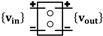
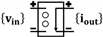
Whatever the terms of the governing equation and its complexity, its simulation can be carried out by means of a network model (electrical circuit) consisting of only a few electrical components: (i) capacitors and resistors to implement the linear terms; and (ii) constant or controlled sources to implement the rest of the terms. Table 2 lists the symbols of all components and their constitutive equations. For resistors and capacitors, the constitutive equations or relationships between the electric current (${\mathrm{i}}_{\mathrm{R}}$) and the potential difference at their ends (${\mathrm{v}}_{\mathrm{R}}$) are ${\mathrm{i}}_{\mathrm{R}}$ = $\frac{{\mathrm{v}}_{\mathrm{R}}}{\mathrm{R}}$ and ${\mathrm{i}}_{\mathrm{C}}$ = $\mathrm{C}${$\frac{\mathrm{d}{\mathrm{v}}_{\mathrm{C}}}{\mathrm{d}\mathrm{t}}$}, respectively. For the correct implementation of the component in the model, the directions of the electric current and the potential difference must be consistent with those indicated in the table. In the constitutive equations of the controlled sources, the output variable (voltage or current, ${\mathrm{v}}_{\mathrm{o}\mathrm{u}\mathrm{t}}$ or ${\mathrm{i}}_{\mathrm{o}\mathrm{u}\mathrm{t}}$) is an arbitrary function—which is defined by programming—of the input variable (voltage or current, ${\mathrm{v}}_{\mathrm{i}\mathrm{n}}$ or ${\mathrm{i}}_{\mathrm{i}\mathrm{n}}$). Constant sources implement constant terms of the equation and time-dependent sources implement time-dependent terms.

Table 2. Electrical components of network models and their constitutive equations.

Component	Symbol	Constitutive Equation
Resistor		${\mathrm{i}}_{\mathrm{R}}=\frac{{\mathrm{v}}_{\mathrm{R}}}{\mathrm{R}}$
Capacitor		${\mathrm{v}}_{\mathrm{C}}=\mathrm{C}\frac{\mathrm{d}{\mathrm{i}}_{\mathrm{C}}}{\mathrm{d}\mathrm{t}}$
Constant voltage source		${\mathrm{v}}_{\mathrm{C}}=\mathrm{c}\mathrm{o}\mathrm{n}\mathrm{s}\mathrm{t}\mathrm{a}\mathrm{n}\mathrm{t}$
Constant current source		${\mathrm{I}}_{\mathrm{C}}=\mathrm{c}\mathrm{o}\mathrm{n}\mathrm{s}\mathrm{t}\mathrm{a}\mathrm{n}\mathrm{t}$
Voltage-controlled voltage-source		${\mathrm{v}}_{\mathrm{o}\mathrm{u}\mathrm{t}}={\mathrm{f}(\mathrm{v}}_{\mathrm{i}\mathrm{n}})$
Voltage-controlled current-source		${\mathrm{i}}_{\mathrm{o}\mathrm{u}\mathrm{t}}={\mathrm{f}(\mathrm{v}}_{\mathrm{i}\mathrm{n}})$
Current-controlled voltage-source		${\mathrm{v}}_{\mathrm{o}\mathrm{u}\mathrm{t}}={\mathrm{f}(\mathrm{i}}_{\mathrm{i}\mathrm{n}})$
Current-controlled current-source		${\mathrm{i}}_{\mathrm{o}\mathrm{u}\mathrm{t}}={\mathrm{f}(\mathrm{i}}_{\mathrm{i}\mathrm{n}})$

There are four types of controlled sources, although the most commonly used are the voltage-controlled current sources, to implement terms of the equation (linear or not) that are a function of the dependent variable, and current-controlled current sources to implement the second- and higher-order derivative terms. For some applications, for example, when the governing equation contains time-dependent terms, it is necessary to implement in the model an auxiliary circuit to define the time variable.

2.1. Basic Circuits

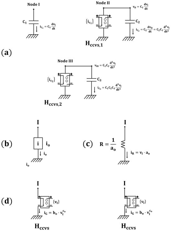
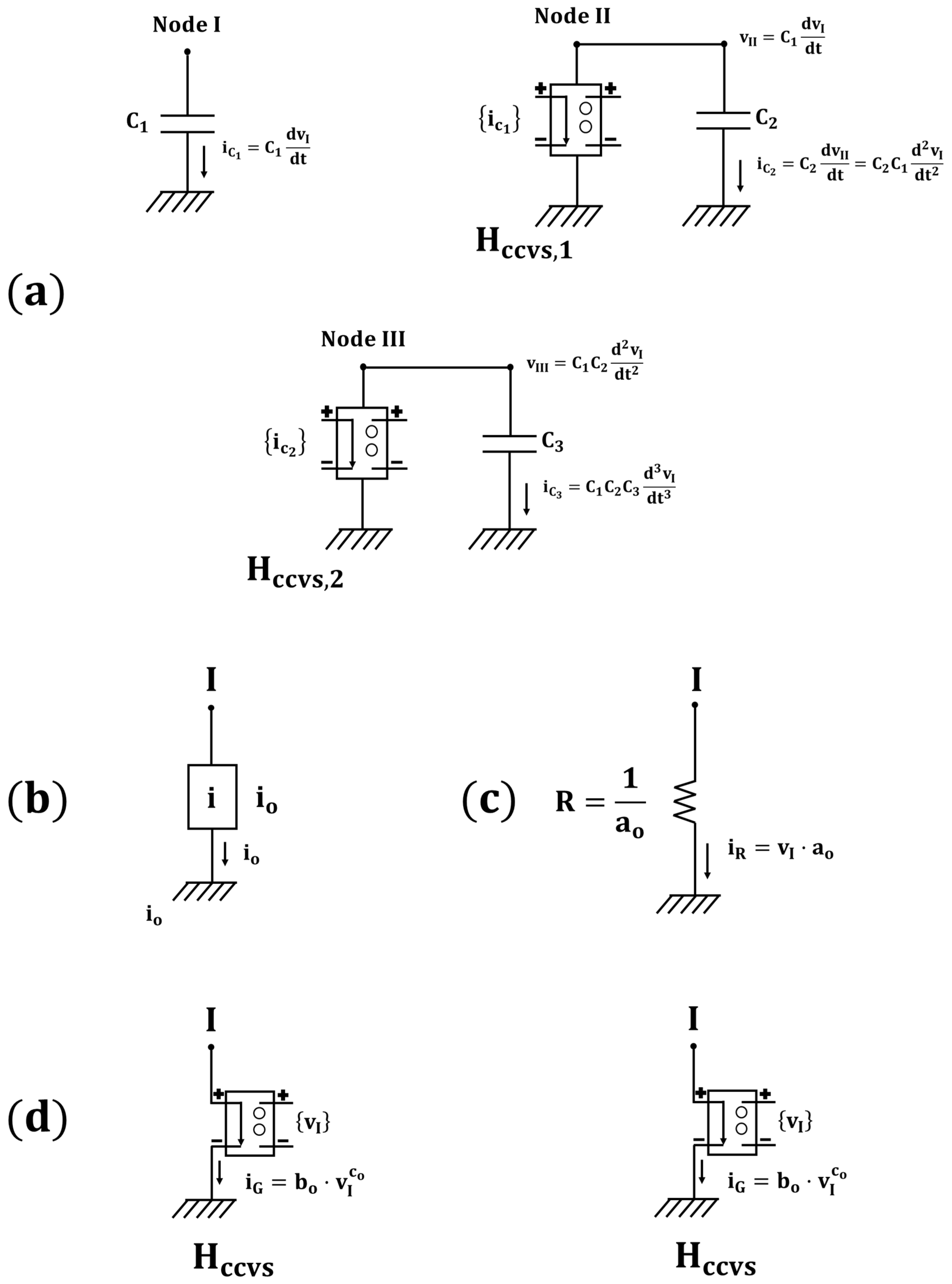
Among the most common summands or terms of a differential equation, we first distinguish the derivative terms. The order of the largest existing derivative classifies the type of equation: first order, second order, etc. Since the solution sought is going to be the voltage ${\mathrm{v}}_{\mathrm{I}}\left(\mathrm{t}\right)$ at the main node of the model (node I), the implementation of a capacitor (${\mathrm{C}}_1$) in one of the branches of the circuit of that node sets a current of value ${\mathrm{i}}_{{\mathrm{C}}_1}$ = ${\mathrm{C}}_1$($\mathrm{d}{\mathrm{v}}_{\mathrm{I}}/\mathrm{d}\mathrm{t}$), which is equivalent to implement the equivalent term of the first derivative (when it exists). The value of ${\mathrm{C}}_1$ allows us to adjust the coefficient of this term to its particular value in the equation. Each of the following derivatives is implemented by two components: a current-controlled voltage generator (${\mathrm{H}}_{\mathrm{c}\mathrm{c}\mathrm{v}\mathrm{s}}$) and a new capacitor ($\mathrm{C}$). For example, the second derivative (node II) does with the pair ${\mathrm{H}}_{\mathrm{c}\mathrm{c}\mathrm{v}\mathrm{s},1}$ and ${\mathrm{C}}_2$. The input of ${\mathrm{H}}_{\mathrm{c}\mathrm{c}\mathrm{v}\mathrm{s},1}$, defined by programming in the source specification, is the current ${\mathrm{i}}_{{\mathrm{C}}_1}$, while the output voltage (connected to the ends of ${\mathrm{C}}_2$) has the same numerical value as that current, i.e., ${\mathrm{v}}_{{\mathrm{H}}_{\mathrm{c}\mathrm{c}\mathrm{v}\mathrm{s},1}}={\mathrm{i}}_{{\mathrm{C}}_1}={\mathrm{C}}_1\left(\frac{\mathrm{d}{\mathrm{v}}_{\mathrm{I}}}{\mathrm{d}\mathrm{t}}\right)$. Thus, the current in ${\mathrm{C}}_2$ is ${\mathrm{i}}_{{\mathrm{C}}_2}$ = ${\mathrm{C}}_2\left(\frac{\mathrm{d}{\mathrm{v}}_{{\mathrm{H}}_{\mathrm{c}\mathrm{c}\mathrm{v}\mathrm{s},1}}}{\mathrm{d}\mathrm{t}}\right)$ = ${\mathrm{C}}_1{\mathrm{C}}_2\{{\mathrm{d}}^2{\mathrm{v}}_{\mathrm{I}}/{\mathrm{d}\mathrm{t}}^2$}, i.e., the second derivative term of the equation. Again, the value of ${\mathrm{C}}_2$ allows for the adjustment of the coefficient of such a term. The third and successive derivative terms follow the same rule for their implementation in the model, using the pair ${\mathrm{C}}_3-{\mathrm{H}}_{\mathrm{c}\mathrm{c}\mathrm{v}\mathrm{s},2}$ to implement the third derivative, and so on. Figure 1a shows these components within the network model.

Figure 1. Implementation of (a) derivative terms, (b) positive constant term, (c) first-degree term of the dependent variable, and (d) nonlinear first-degree term in the dependent variable.

The independent term of constant value is implemented directly by a constant-current generator ($\mathrm{I}$) with a sense consistent with the algebraic sign of the term in the equation. Figure 1b implements a constant-valued term of numerical value equal to that of the generator current, ${\mathrm{i}}_{\mathrm{G}}$. A term of the form ${\mathrm{a}}_{\mathrm{o}}\mathrm{x}$ (with $\mathrm{x}$ the dependent variable, ${\mathrm{v}}_{\mathrm{I}}$) is implemented, according to its constitutive equation, by a resistor ($\mathrm{R}$) of value $\mathrm{R}$ = $1/{\mathrm{a}}_{\mathrm{o}}$, as shown in Figure 1c. The remaining terms are always implemented with a new ${\mathrm{H}}_{\mathrm{c}\mathrm{c}\mathrm{v}\mathrm{s}}$, and as many as there are summands in the equation. The expression of these terms, sometimes complex, may require auxiliary circuits for implementation. Figure 1d implements a term of the form ${\mathrm{b}}_{\mathrm{o}}{\mathrm{x}}^{{\mathrm{c}}_{\mathrm{o}}}$. The output current of the generator ${\mathrm{H}}_{\mathrm{c}\mathrm{c}\mathrm{v}\mathrm{s}}$ (defined by programming) is ${\mathrm{i}}_{{\mathrm{H}}_{\mathrm{c}\mathrm{c}\mathrm{v}\mathrm{s}}}$ = ${\mathrm{b}}_{\mathrm{o}}{\mathrm{x}}^{{\mathrm{c}}_{\mathrm{o}}}$ = ${\mathrm{b}}_{\mathrm{o}}{\mathrm{v}}_{\mathrm{I}}^{{\mathrm{c}}_{\mathrm{o}}}$. Other examples are shown in the Section 3.

2.2. Text Files

The model can be entered into the program using the schematics tool included in the software itself, which uses the standard circuit theory symbols, or through a text file using a minimal set of writing rules. For resistors, capacitors, and constant sources, it is sufficient to indicate their name, the nodes of the circuit to which they are connected, and their value, and for controlled sources, their name, the nodes or element from which they read the input, the nodes where their output is connected, and the control function that is specified by programming. Table 3 shows the specification of the text lines corresponding to the elements listed in Table 2 (Pspice [23]). In the Section 3, the text files of the studied models are shown and explained.

Table 3. Lines of the text file specifying the electrical components of the network model.

Component	Sentence
	Symbol	Connection Nodes		Value
		Input	Output
Resistor	$\mathrm{R}$	${\mathrm{R}}_{\mathrm{I}}$	${\mathrm{R}}_{\mathrm{I}\mathrm{I}}$	${\mathrm{R}}_{\mathrm{o}}$
Capacitor	$\mathrm{C}$	${\mathrm{C}}_{\mathrm{I}}$	${\mathrm{C}}_{\mathrm{I}\mathrm{I}}$	${\mathrm{C}}_{\mathrm{o}}$
Constant voltage source	$\mathrm{v}$	${\mathrm{v}}_{\mathrm{I}}$	${\mathrm{v}}_{\mathrm{I}\mathrm{I}}$	${\mathrm{v}}_{\mathrm{o}}$
Constant current source	$\mathrm{i}$	${\mathrm{i}}_{\mathrm{I}}$	${\mathrm{i}}_{\mathrm{I}\mathrm{I}}$	${\mathrm{i}}_{\mathrm{o}}$
Voltage-controlled voltage-source	$\mathrm{E}$	${\mathrm{E}}_{\mathrm{I},\mathrm{i}\mathrm{n}}$  ${\mathrm{E}}_{\mathrm{I}\mathrm{I},\mathrm{i}\mathrm{n}}$	${\mathrm{E}}_{\mathrm{I},\mathrm{o}\mathrm{u}\mathrm{t}}$  ${\mathrm{E}}_{\mathrm{I}\mathrm{I},\mathrm{o}\mathrm{u}\mathrm{t}}$	${\mathrm{v}}_{\mathrm{o}\mathrm{u}\mathrm{t}}={\mathrm{f}(\mathrm{v}}_{\mathrm{i}\mathrm{n}})$
Voltage-controlled current-source	$\mathrm{G}$	${\mathrm{G}}_{\mathrm{I},\mathrm{i}\mathrm{n}}$  ${\mathrm{G}}_{\mathrm{I}\mathrm{I},\mathrm{i}\mathrm{n}}$	${\mathrm{G}}_{\mathrm{I},\mathrm{o}\mathrm{u}\mathrm{t}}$  ${\mathrm{G}}_{\mathrm{I}\mathrm{I},\mathrm{o}\mathrm{u}\mathrm{t}}$	${\mathrm{i}}_{\mathrm{o}\mathrm{u}\mathrm{t}}={\mathrm{f}(\mathrm{v}}_{\mathrm{i}\mathrm{n}})$
Current-controlled voltage-source	$\mathrm{H}$	${\mathrm{H}}_{\mathrm{I},\mathrm{i}\mathrm{n}}$  ${\mathrm{H}}_{\mathrm{I}\mathrm{I},\mathrm{i}\mathrm{n}}$	${\mathrm{H}}_{\mathrm{I},\mathrm{o}\mathrm{u}\mathrm{t}}$  ${\mathrm{H}}_{\mathrm{I}\mathrm{I},\mathrm{o}\mathrm{u}\mathrm{t}}$	${\mathrm{v}}_{\mathrm{o}\mathrm{u}\mathrm{t}}={\mathrm{f}(\mathrm{i}}_{\mathrm{i}\mathrm{n}})$
Current-controlled current-source	$\mathrm{F}$	${\mathrm{F}}_{\mathrm{I},\mathrm{i}\mathrm{n}}$  ${\mathrm{F}}_{\mathrm{I}\mathrm{I},\mathrm{i}\mathrm{n}}$	${\mathrm{F}}_{\mathrm{I},\mathrm{o}\mathrm{u}\mathrm{t}}$  ${\mathrm{F}}_{\mathrm{I}\mathrm{I},\mathrm{o}\mathrm{u}\mathrm{t}}$	${\mathrm{i}}_{\mathrm{o}\mathrm{u}\mathrm{t}}={\mathrm{f}(\mathrm{i}}_{\mathrm{i}\mathrm{n}})$

3. Applications and Simulation

Three applications to mechanical and chaotic dynamic processes have been selected that sufficiently illustrate the application of the protocol of the network simulation method. These processes contain in their governing equations both linear and nonlinear summands—terms in the first and second derivative, terms as a function of the dependent variable, rational exponents, etc.—and can therefore be taken as very representative of any kind of dynamic process. For each application, the design of the network model is described in detail, showing its text file to be read and executed in the software. The simulation results obtained with the graphical output environment of the software itself are also briefly discussed.

3.1. Mass Falling in Air or Viscous Fluid

This simple process, ruled by a differential equation of three addends and nonlinear because of the existence of the exponent b_o in general different from unity, governs the motion of a mass falling in air or viscous fluid. It is also named the skydiver equation, as it governs the movement of a parachutist falling towards the earth by the action of gravitational force but slowed down by air friction with a force dependent on the instantaneous velocity. The balance of forces (Newton’s second law) is given by the equation $\sum \mathrm{f}=\mathrm{W}\mathrm{e}\mathrm{i}\mathrm{g}\mathrm{h}\mathrm{t}-{\mathrm{f}}_{\mathrm{f}\mathrm{r}\mathrm{i}\mathrm{c}\mathrm{t}\mathrm{i}\mathrm{o}\mathrm{n}}=\mathrm{m}\frac{{\mathrm{d}}^2\mathrm{x}}{\mathrm{d}{\mathrm{t}}^2}$. With $\mathrm{P}=\mathrm{m}\mathrm{g}$, and expressing the frictional force in the form ${\mathrm{f}}_{\mathrm{f}\mathrm{r}\mathrm{i}\mathrm{c}\mathrm{t}\mathrm{i}\mathrm{o}\mathrm{n}}=\mathsf{\gamma }{\mathrm{v}}^{{\mathrm{a}}_{\mathrm{o}}}=\mathsf{\gamma }{\left(\frac{\mathrm{d}\mathrm{x}}{\mathrm{d}\mathrm{t}}\right)}^{{\mathrm{a}}_{\mathrm{o}}}$, the balance equation yields

$$\frac{{\mathrm{d}}^2\mathrm{x}}{\mathrm{d}{\mathrm{t}}^2}+\frac{\mathsf{\gamma }}{\mathrm{m}}{\left(\frac{\mathrm{d}\mathrm{x}}{\mathrm{d}\mathrm{t}}\right)}^{{\mathrm{a}}_{\mathrm{o}}}-\mathrm{g}=0,$$

(1)

with $\mathrm{m}$ the mass of the parachutist, $\mathrm{v}$ its instantaneous velocity, $\mathrm{g}$ the acceleration of gravity, $\mathsf{\gamma }$ and ${\mathrm{a}}_{\mathrm{o}}$ constants of the friction force expression, and $\mathrm{x}$ the dependent variable position. The initial conditions are: ${\mathrm{x}}_{\mathrm{t}=0}={\mathrm{v}}_{\mathrm{t}=0}=0$.

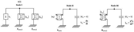
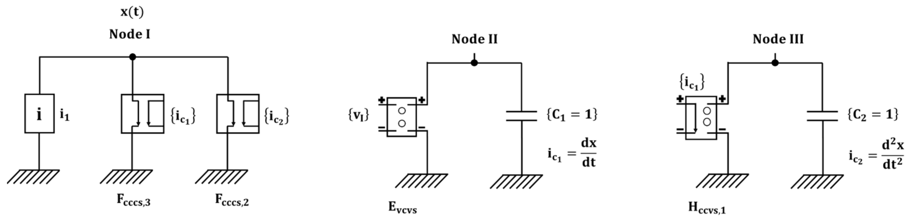
The network model, shown in Figure 2, consists of a main circuit (node I) with three branches corresponding to the three summands of the equation and two auxiliary circuits (nodes II and III), which implement the first and second derivatives. The solution to the problem is the main node voltage, $\mathrm{x}\left(\mathrm{t}\right)={\mathrm{v}}_{\mathrm{I}}\left(\mathrm{t}\right)$. In the first auxiliary circuit, formed by ${\mathrm{E}}_{\mathrm{v}\mathrm{c}\mathrm{v}\mathrm{s},1}$ and ${\mathrm{C}}_1$, with ${\mathrm{C}}_1=1$, the generator output current is equal to the input voltage, ${\mathrm{i}}_{{\mathrm{E}}_{\mathrm{v}\mathrm{c}\mathrm{v}\mathrm{s},1}}={\mathrm{v}}_{\mathrm{I}}$, so ${\mathrm{i}}_{{\mathrm{C}}_1}={\mathrm{C}}_1\frac{\mathrm{d}{\mathrm{v}}_{\mathrm{I}}}{\mathrm{d}\mathrm{t}}=\frac{\mathrm{d}\mathrm{x}}{\mathrm{d}\mathrm{t}}$. The second auxiliary circuit consists of ${\mathrm{H}}_{\mathrm{c}\mathrm{c}\mathrm{v}\mathrm{s},1}$ and ${\mathrm{C}}_2$, with ${\mathrm{C}}_2=1$. The output current of this controlled source (${\mathrm{i}}_{{\mathrm{H}}_{\mathrm{c}\mathrm{c}\mathrm{v}\mathrm{s},1,\mathrm{o}\mathrm{u}\mathrm{t}}}={\mathrm{i}}_{{\mathrm{C}}_2}$) has the same value as the current ${\mathrm{i}}_{{\mathrm{C}}_1}$. Thus, ${\mathrm{i}}_{{\mathrm{H}}_{\mathrm{c}\mathrm{c}\mathrm{v}\mathrm{s},1,\mathrm{o}\mathrm{u}\mathrm{t}}}={\mathrm{C}}_2\frac{\mathrm{d}{\mathrm{v}}_{\mathrm{N}\mathrm{o}\mathrm{d}\mathrm{e}\mathrm{I}\mathrm{I}\mathrm{I}}}{\mathrm{d}\mathrm{t}}=\frac{{\mathrm{d}}^2\mathrm{x}}{\mathrm{d}{\mathrm{t}}^2}$.

Figure 2. Network model of the mass falling in air or viscous fluid.

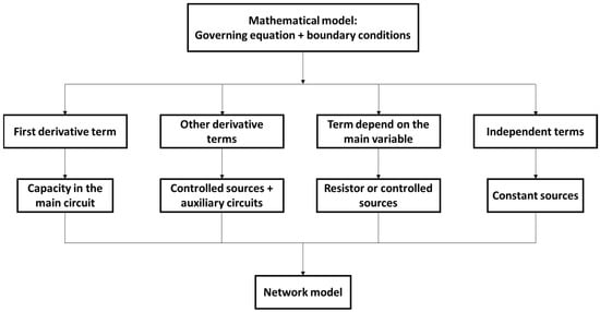
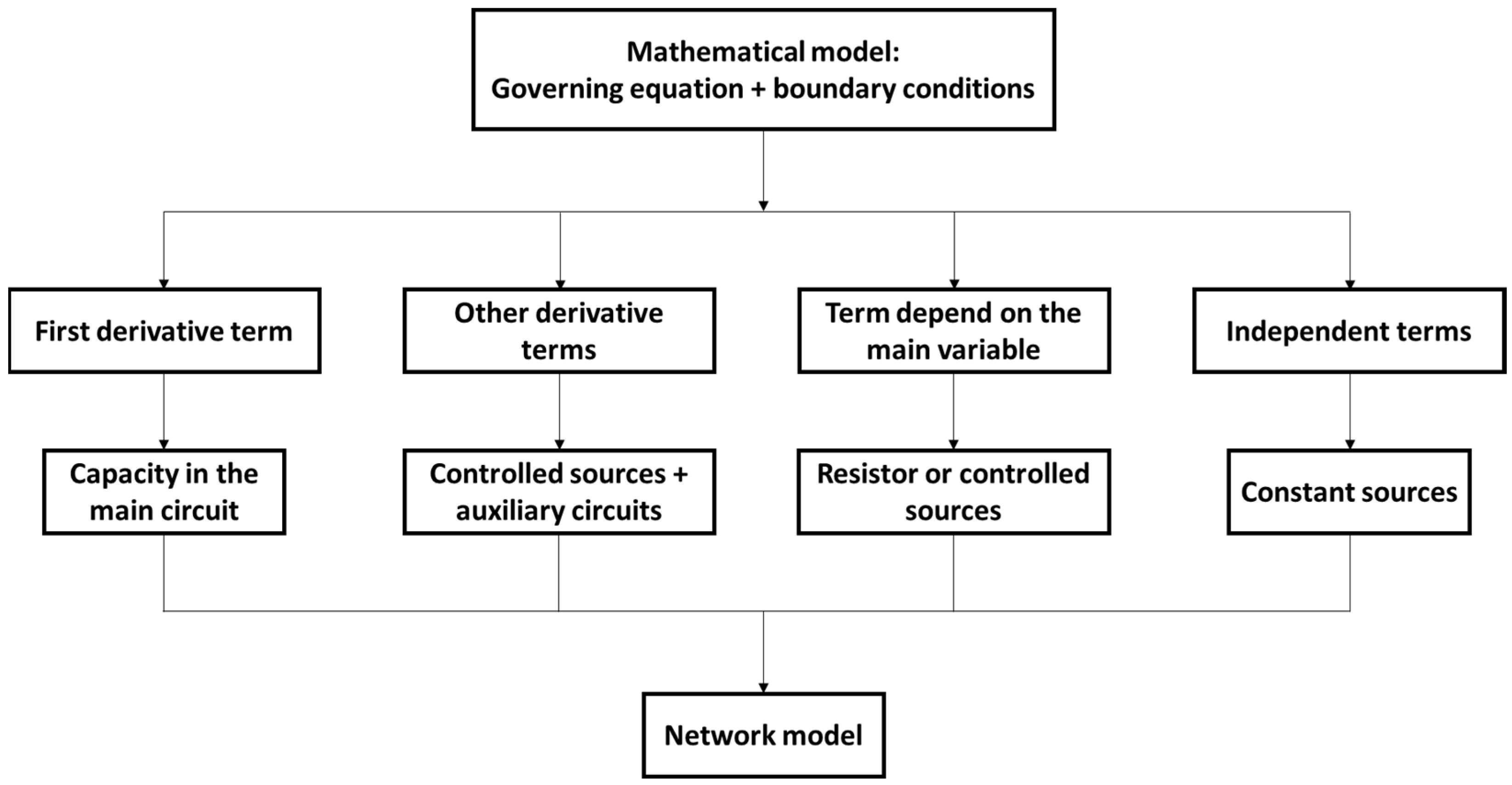
Having the first derivatives as currents in ${\mathrm{C}}_1$ and ${\mathrm{C}}_2$, ${\mathrm{i}}_{{\mathrm{C}}_1}=$ $\frac{\mathrm{d}\mathrm{x}}{\mathrm{d}\mathrm{t}}$ and ${\mathrm{i}}_{{\mathrm{C}}_2}=\frac{{\mathrm{d}}^2\mathrm{x}}{\mathrm{d}{\mathrm{t}}^2}$, it is immediate to implement the branches of the main circuit corresponding to the summands $\frac{{\mathrm{d}}^2\mathrm{x}}{\mathrm{d}{\mathrm{t}}^2}$ and $\frac{\mathsf{\gamma }}{\mathrm{m}}{\left(\frac{\mathrm{d}\mathrm{x}}{\mathrm{d}\mathrm{t}}\right)}^{{\mathrm{a}}_{\mathrm{o}}}$. The first contains generator ${\mathrm{F}}_{\mathrm{c}\mathrm{c}\mathrm{c}\mathrm{s},2}$, whose input and output have the same value, ${\mathrm{i}}_{\mathrm{o}\mathrm{u}\mathrm{t},{\mathrm{F}}_{\mathrm{c}\mathrm{c}\mathrm{c}\mathrm{s},2}}$ = ${\mathrm{i}}_{\mathrm{i}\mathrm{n},{\mathrm{F}}_{\mathrm{c}\mathrm{c}\mathrm{c}\mathrm{s},2}}$= ${\mathrm{i}}_{{\mathrm{C}}_2}$ = $\frac{{\mathrm{d}}^2\mathrm{x}}{\mathrm{d}{\mathrm{t}}^2}$. The second contains generator ${\mathrm{F}}_{\mathrm{c}\mathrm{c}\mathrm{c}\mathrm{s},3}$, whose input is ${\mathrm{i}}_{\mathrm{i}\mathrm{n},{\mathrm{F}}_{\mathrm{c}\mathrm{c}\mathrm{c}\mathrm{s},3}}$ = ${\mathrm{i}}_{{\mathrm{C}}_1}$ = $\frac{\mathrm{d}\mathrm{x}}{\mathrm{d}\mathrm{t}}$, and with output a function of this value defined by programming, ${\mathrm{i}}_{\mathrm{o}\mathrm{u}\mathrm{t},{\mathrm{F}}_{\mathrm{c}\mathrm{c}\mathrm{c}\mathrm{s},3}}$= $\frac{\mathsf{\gamma }}{\mathrm{m}}{\left({\mathrm{i}}_{\mathrm{i}\mathrm{n},{\mathrm{F}}_{\mathrm{c}\mathrm{c}\mathrm{c}\mathrm{s},3}}\right)}^{{\mathrm{a}}_{\mathrm{o}}}=\frac{\mathsf{\gamma }}{\mathrm{m}}{\left(\frac{\mathrm{d}\mathrm{x}}{\mathrm{d}\mathrm{t}}\right)}^{{\mathrm{a}}_{\mathrm{o}}}$. Finally, the constant term $\mathrm{g}$ is implemented with the constant current generator ${\mathrm{I}}_1$ towards the main node (because of the negative sign), ${\mathrm{i}}_{\mathrm{o}\mathrm{u}\mathrm{t},{\mathrm{I}}_1}$ = $\mathrm{g}$. Figure 2 shows the network model of the problem. The initial conditions of position and velocity, ${\mathrm{x}}_{\mathrm{i}\mathrm{n}\mathrm{i}}$ and ${\mathrm{v}}_{\mathrm{i}\mathrm{n}\mathrm{i}}$, are applied as initial voltage on capacitors ${\mathrm{C}}_1$ and ${\mathrm{C}}_2$, ${\mathrm{v}}_{\mathrm{i}\mathrm{n}\mathrm{i},{\mathrm{C}}_1}$ = ${\mathrm{v}}_{\mathrm{t}=0}$ = 0, and ${\mathrm{v}}_{\mathrm{i}\mathrm{n}\mathrm{i},{\mathrm{C}}_2}$ = ${\mathrm{x}}_{\mathrm{t}=0}$ = 0, respectively. The flow chart in Figure 3 explains the procedure for creating the network model text file.

Figure 3. Flow chart for creating the network model text file.

The text file of the model is as follows:

• *Solution of ordinary differential equations
• *Governing equation: m × g − (γ) × (${\mathrm{v}}^{{\mathrm{a}}_{\mathrm{o}}}$) − m × a = 0.
• G1 I 0 VALUE = {m × g}
• G_cccs,3 I 0 VALUE = {γ × ${\mathrm{v}}^{{\mathrm{a}}_{\mathrm{o}}}$}
• G_cccs,2 0 I VALUE = {m × a}
• G_vccs,1 II 0 VALUE = {V(I)}
• C1 II 0 1
• G_cccs,1 III 0 VALUE = {i_C1}
• C2 III 0 1
• V_time 100 0 PWL(0,0 500,500)
• .TRAN 1 s 1.5 s 0 UIC
• .END

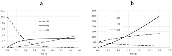
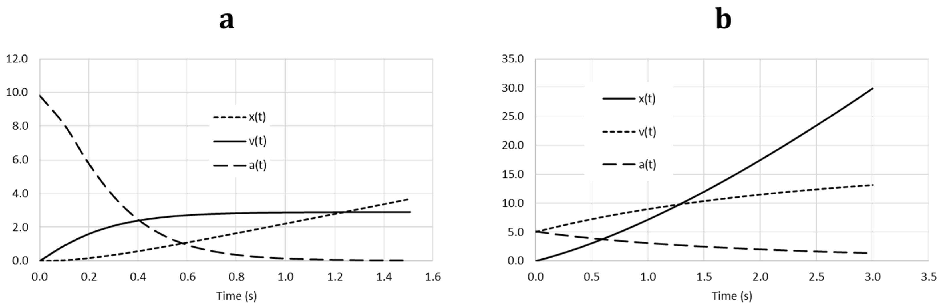
The asterisk implies that this line of text is not executed by the program. In the voltage source, time is read is ${\mathrm{v}}_{\mathrm{t}\mathrm{i}\mathrm{m}\mathrm{e}}$, while the sentence ‘.TRANS’ specifies the time interval to be simulated. The curves in Figure 4, in the Pspice graphical environment, show the simulation results—position ($\mathrm{x}$), velocity ($\mathrm{v}$) and acceleration (a), as a function of time—for the parameters g = 9.81, m = 1, ${\mathrm{x}}_{\mathrm{i}\mathrm{n}\mathrm{i}}$ = 0, $\mathsf{\gamma }$ = 2 and 1.8, ${\mathrm{a}}_{\mathrm{o}}$ = 1.5 and 0.6, and ${\mathrm{v}}_{\mathrm{i}\mathrm{n}\mathrm{i}}$ = 0 and 5. Note that in both cases, as expected, the location increases monotonically until lineal, and velocity increases progressively until a steady value is reached and acceleration diminished, converging to a zero value. Initial conditions determine the starting point of the curves.

Figure 4. Simulation results of the mass falling in a viscous fluid. (a): g = 9.81, $\mathsf{\gamma }$ = 2, m = 1, ${\mathrm{a}}_{\mathrm{o}}$ = 1.5, ${\mathrm{x}}_{\mathrm{i}\mathrm{n}\mathrm{i}}$ = ${\mathrm{v}}_{\mathrm{i}\mathrm{n}\mathrm{i}}$ = 0. (b): g = 9.81, $\mathsf{\gamma }$ = 1.8 m = 1, ${\mathrm{a}}_{\mathrm{o}}$ = 0.6, ${\mathrm{x}}_{\mathrm{i}\mathrm{n}\mathrm{i}}$ = 0, ${\mathrm{v}}_{\mathrm{i}\mathrm{n}\mathrm{i}}$ = 5.

3.2. Crimped Bead Sliding on a Parabolic Shaped Wire

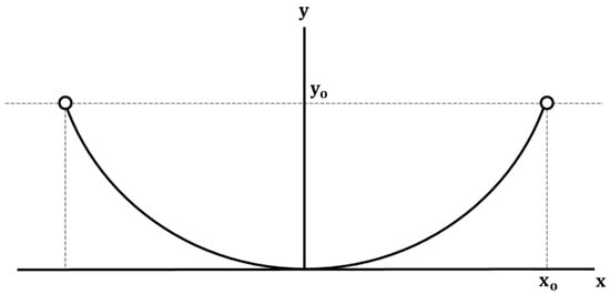
In Figure 5, by the action of gravity, the ball attached to the wire falls (sliding without friction) following the parabolic trajectory $\mathrm{y}={\mathrm{a}}_{\mathrm{o}}{\mathrm{x}}^2$. The balance between the gravitational force and the normal reaction of the wire (Newton’s law) allows us to write the governing equation in the following form:

$$\left(\frac{{\mathrm{d}}^2\mathrm{x}}{\mathrm{d}{\mathrm{t}}^2}\right)\left(1+{\mathrm{a}}_{\mathrm{o}}{\mathrm{x}}^2\right)+{\mathrm{a}}_{\mathrm{o}}\mathrm{x}{\left(\frac{\mathrm{d}\mathrm{x}}{\mathrm{d}\mathrm{t}}\right)}^2+{\mathrm{b}}_{\mathrm{o}}\mathrm{x}=0,$$

(2)

Figure 5. Sliding bead strung on a fixed wire.

The mathematical model is completed with the initial conditions that we will choose simply, as ${\mathrm{x}}_{\mathrm{t}=0}=5$ and ${\mathrm{v}}_{\mathrm{t}=0}=0$. The position y(t) is given by the trajectory equation once the solution x(t) is obtained.

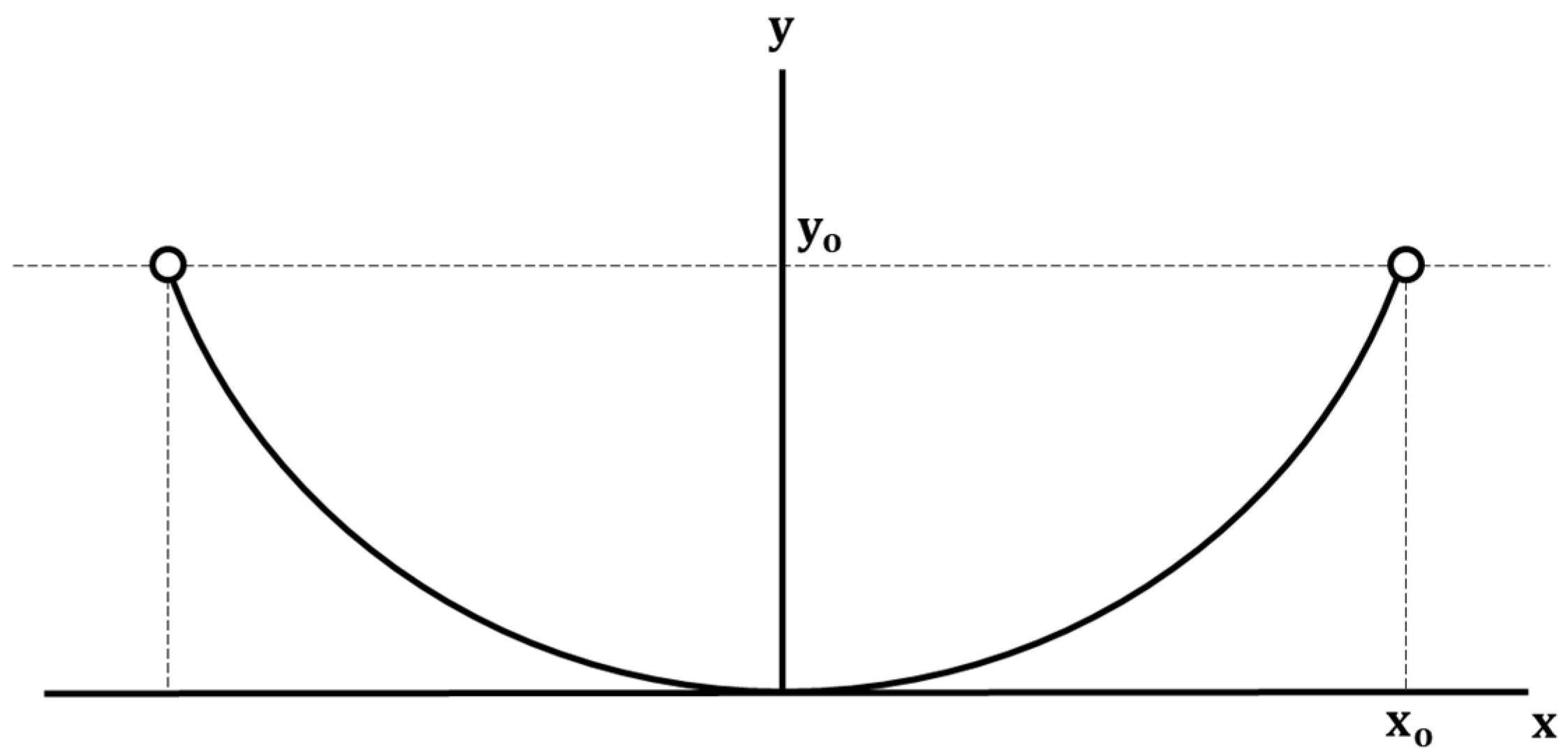
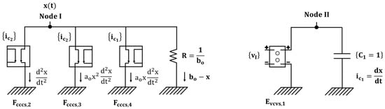
The network model is shown in Figure 6. The derivative factors $\left(\frac{\mathrm{d}\mathrm{x}}{\mathrm{d}\mathrm{t}}\right)$ and $\left(\frac{{\mathrm{d}}^2\mathrm{x}}{\mathrm{d}{\mathrm{t}}^2}\right)$ are implemented with circuits similar to those explained in the previous application, auxiliary circuits of nodes II and III. The terms $\left(\frac{{\mathrm{d}}^2\mathrm{x}}{\mathrm{d}{\mathrm{t}}^2}\right)$ and ${\mathrm{a}}_{\mathrm{o}}{\mathrm{x}}^2\left(\frac{{\mathrm{d}}^2\mathrm{x}}{\mathrm{d}{\mathrm{t}}^2}\right)$ are implemented in the main circuit by the current generators ${\mathrm{F}}_{\mathrm{c}\mathrm{c}\mathrm{c}\mathrm{s},2}$ and ${\mathrm{F}}_{\mathrm{c}\mathrm{c}\mathrm{c}\mathrm{s},3}$, the term ${\mathrm{a}}_{\mathrm{o}}\mathrm{x}{\left(\frac{\mathrm{d}\mathrm{x}}{\mathrm{d}\mathrm{t}}\right)}^2$ is implemented by ${\mathrm{F}}_{\mathrm{c}\mathrm{c}\mathrm{c}\mathrm{s},4}$, and finally, the term ${\mathrm{b}}_{\mathrm{o}}\mathrm{x}$ is implemented by a resistor of value $\mathrm{R}=1/{\mathrm{b}}_{\mathrm{o}}$.

Figure 6. Network model of the bead crimped to the wire.

The text file of the model is as follows:

• *Solution of ordinary differential equations
• *Governing equation: $\left(\frac{{\mathrm{d}}^2\mathrm{x}}{\mathrm{d}{\mathrm{t}}^2}\right)\left(1+{\mathrm{a}}_{\mathrm{o}}{\mathrm{x}}^2\right)+{\mathrm{a}}_{\mathrm{o}}\mathrm{x}{\left(\frac{\mathrm{d}\mathrm{x}}{\mathrm{d}\mathrm{t}}\right)}^2+{\mathrm{b}}_{\mathrm{o}}\mathrm{x}=0$
• G_cccs,2 I 0 VALUE = {$\frac{{\mathrm{d}}^2\mathrm{x}}{\mathrm{d}{\mathrm{t}}^2}$}
• G_cccs,3 I 0 VALUE = {${\mathrm{a}}_{\mathrm{o}}{\mathrm{x}}^2\frac{{\mathrm{d}}^2\mathrm{x}}{\mathrm{d}{\mathrm{t}}^2}$}
• G_cccs,4 I 0 VALUE = {${\mathrm{a}}_{\mathrm{o}}\mathrm{x}{\left(\frac{\mathrm{d}\mathrm{x}}{\mathrm{d}\mathrm{t}}\right)}^2$}
• R 1 0 b_o⁻¹
• G_vcvs,1 II 0 VALUE = {V(I)}
• C1 II 0 1
• G_vccs,1 III 0 VALUE = {iC1}
• C2 III 0 1
• .TRAN 1 s 50 s 0 UIC
• .END

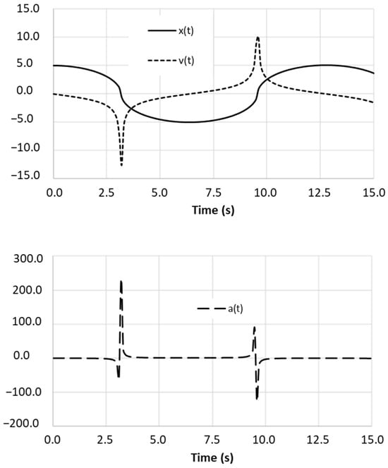
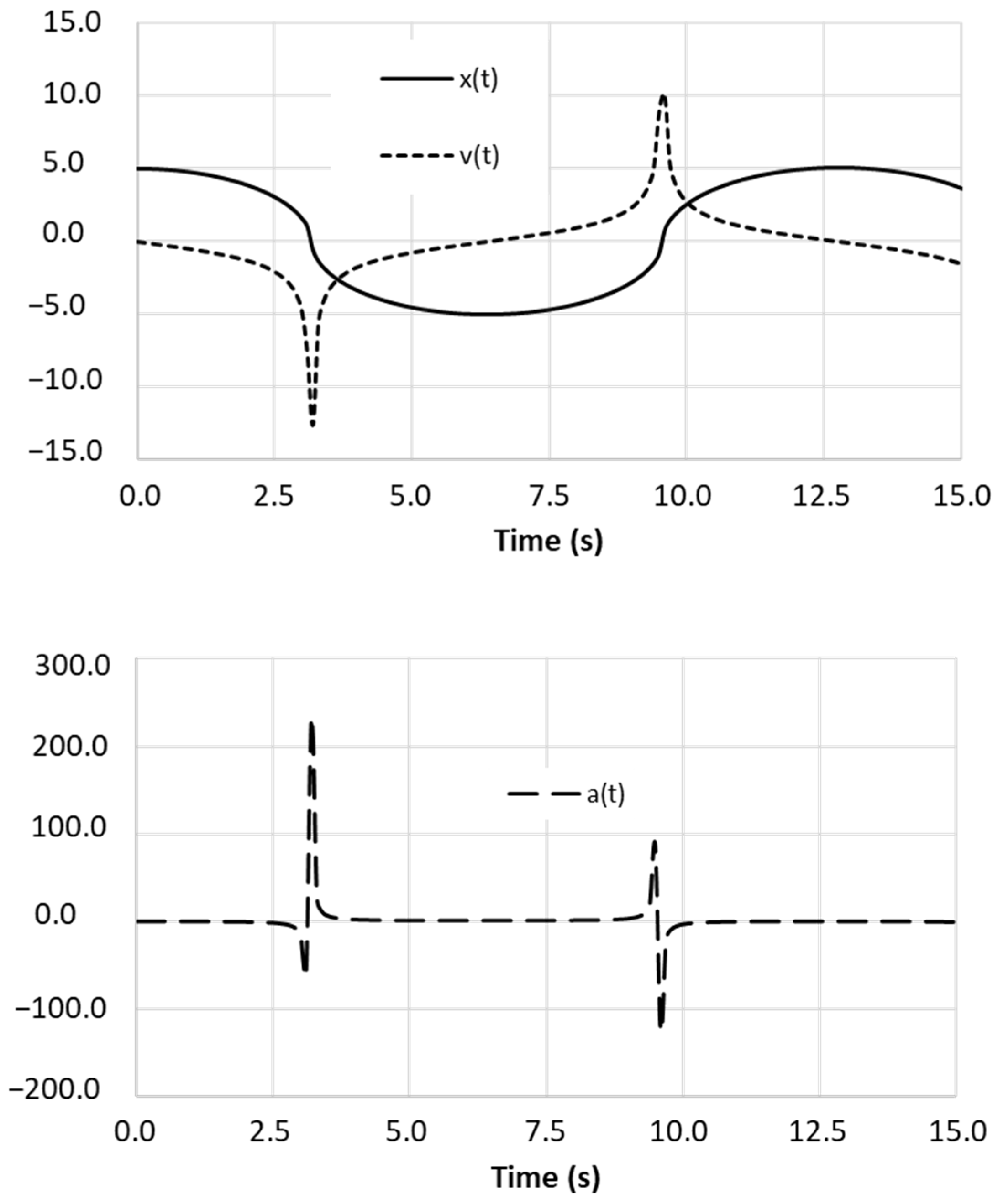
Figure 7 shows the solutions x(t) and v(t) (above figure), and a(t) (below figure), of the problem for the following values of its parameters: m = 1, b = 2, g = 10, ${\mathrm{x}}_{\mathrm{i}\mathrm{n}\mathrm{i}}$ = 5, and ${\mathrm{v}}_{\mathrm{i}\mathrm{n}\mathrm{i}}$ = 0. Curves show a clear influence of the nonlinear terms of the equation. On the one hand, as it is an undamped harmonic motion, there is no loss of energy due to friction, so the height reached by the ball at the ends of the motion is the same and its value is a_o${\left({\mathrm{x}}_{\mathrm{t}=0}\right)}^2$. Because of the symmetry of the parabola, the maximum and minimum horizontal positions are also the same and their absolute value is ${\mathrm{x}}_{\mathrm{t}=0}$. On the other hand, Table 4 shows the influence of the parameters a_o and b_o on the maximum velocity (which occurs at x = 0) and on the oscillation period (τ). While the coefficient b_o associated with the elastic restoring force is a clear determinant of the maximum velocity, the coefficient a_o, which affects the concavity of the parabola, does not influence this velocity. As for the period of oscillation, it decreases with increasing b_o and increases with increasing a_o.

Figure 7. Dynamic solutions of the motion of the bead strung on a wire.

Table 4. Influence of parameters a_o and b_o on solutions ${\mathrm{x}}_{\mathrm{m}\mathrm{a}\mathrm{x}}$, ${\mathrm{y}}_{\mathrm{m}\mathrm{a}\mathrm{x}}$, ${\mathrm{v}}_{\mathrm{m}\mathrm{a}\mathrm{x}}$, and τ.

${\mathrm{a}}_{\mathrm{o}}$	4.00	4.00	4.00	1.00	2.00	3.00
${\mathrm{b}}_{\mathrm{o}}$	1.00	2.00	3.00	1.00	1.00	1.00
${\mathrm{x}}_{\mathrm{m}\mathrm{a}\mathrm{x}}$(m)	5.00	5.00	5.00	5.00	5.00	5.00
${\mathrm{y}}_{\mathrm{m}\mathrm{a}\mathrm{x}}$(m)	100.00	100.00	100.00	25.00	50.00	75.00
${\mathrm{v}}_{\mathrm{m}\mathrm{a}\mathrm{x}}$(m·s−1)	22.53	31.77	39.00	22.53	22.53	22.53
τ (s)	8.15	6.48	5.28	4.76	6.57	7.96

3.3. The van der Pol Oscillator

The mathematical model of this nonlinear oscillator [26] is

$$\frac{{\mathrm{d}}^2\mathrm{x}}{\mathrm{d}{\mathrm{t}}^2}-{\mathrm{x}}^2\left(\frac{\mathrm{d}\mathrm{x}}{\mathrm{d}\mathrm{t}}\right)+\mathrm{x}+1=0,$$

(3)

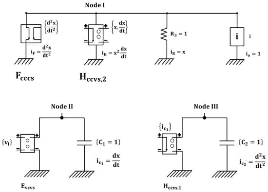
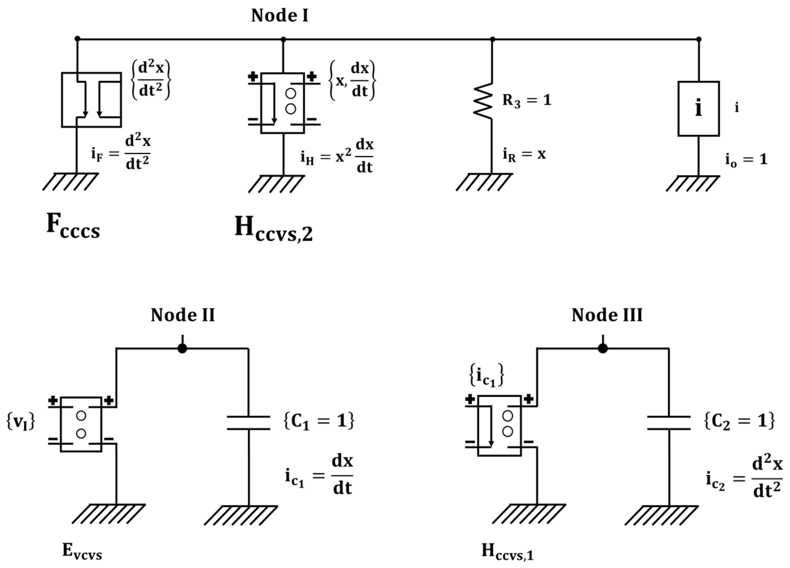
with the initial conditions ${\mathrm{v}}_{\mathrm{t}=0}={\mathrm{v}}_{\mathrm{o}}$ and ${\mathrm{x}}_{\mathrm{t}=0}={\mathrm{x}}_{\mathrm{o}}$, respectively. The network model, shown in Figure 8, which retains the auxiliary circuits of the first application (to implement the current $\frac{{\mathrm{d}}^2\mathrm{x}}{\mathrm{d}{\mathrm{t}}^2}$) and of the second (to implement the voltage $\frac{\mathrm{d}\mathrm{x}}{\mathrm{d}\mathrm{t}}$), has four branches in its main circuit (node I). The first one implements the term $\frac{{\mathrm{d}}^2\mathrm{x}}{\mathrm{d}{\mathrm{t}}^2}$ through the controlled source F_cccs. The second branch, which implement the term ${\mathrm{x}}^2$($\frac{\mathrm{d}\mathrm{x}}{\mathrm{d}\mathrm{t}}$) through the controlled source H_ccvs,2, is controlled by the voltages ${\mathrm{v}}_{\mathrm{I}}=\mathrm{x}$ and ${\mathrm{v}}_{\mathrm{I}\mathrm{I}\mathrm{I}}=\frac{\mathrm{d}\mathrm{x}}{\mathrm{d}\mathrm{t}}$, according to the mathematical expression of the term. The summand x is implemented directly by a resistor (${\mathrm{R}}_3$) of unity value, while the independent term is implemented by the constant current generator Io, whose output is ${\mathrm{i}}_{{\mathrm{i}}_{\mathrm{o}}}=1$.

Figure 8. Network model of the van der Pol oscillator.

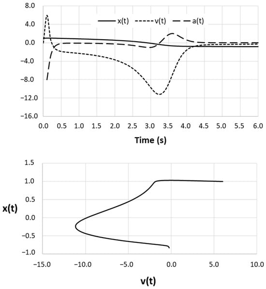
The solutions for position, velocity, and acceleration evolution over time and the position versus velocity phase diagram are shown in Figure 9. For the initial conditions imposed, the motion of this oscillator converges over time to a point where both velocity and acceleration cancel out after a run where these variables oscillate chaotically.

Figure 9. Dynamic solutions of van der Pol’s oscillator.

4. Discussions and Conclusions

The numerical solution of differential equations is not currently a problem for students or researchers thanks to the existence of specific software capable of reliably solving any type of equation, linear or nonlinear. However, the application of this software does not allow the user to deepen complementary aspects of knowledge such as the physical meaning of each term of the equation and its direct effect on the solution. The network models based on the electrical analogy proposed in this work, and the necessary association between physical and electrical variables that such an analogy entails for the elaboration of the model, allows the user to delve into and better understand the phenomenological and physical aspects involved in the governing equation. For this reason, the protocol proposed to design the network model can be considered a powerful educational tool, as it allows students unfamiliar with numerical or differential calculus techniques to easily access the solution and understand the physical processes once the numerical simulation has been carried out.

The design of network models (electrical circuits) has proven to be a useful and accurate tool for simulating a wide range of dynamic processes. The design protocol presented in this work, based on the elementary rules of circuit theory and the constitutive equations of its basic components, includes the incorporation of so-called controlled current or voltage generators. These are capable of implementing in the model any type of summands of the governing equation, such as nonlinear second-order derivative terms, terms that depend on time or on the main variable, etc. Each term of the equation is assumed as an electric current that balances at a common node with the currents of the other terms. The fulfillment of such balancing imposes a unique instantaneous value on the voltage at that node, a value that is the solution to the problem.

The numerical solution is carried out by standard circuit simulation software, such as Pspice. There are two main advantages in the use of electric models: (i) few rules are needed for the design, as the elements that compose the model are very few (resistors, capacitors, and constant or controlled sources); and (ii) the use of powerful computer algorithms contained in these programs, meaning the numerical computation provides a quasi-exact solution to the network model. In addition, the graphical output environment of these programs offers the user an immediate representation of the solutions from which the temporal evolution of the variables, phase diagrams, spectral representation of the harmonic responses, etc., can be selected.

The applications of the proposed protocol to two problems of nonlinear dynamics and one of chaotic motion illustrate the advantages mentioned in the previous paragraph. In all three cases, it is immediate to infer first the dependence of the unknowns of interest, position, velocity, and acceleration on the parameters of the equation, and second, the convergence or not of these unknowns to a stationary final position.

References

- Kirchhoff, S. Ueber den Durchgang eines elektrischen Stromes durch eine Ebene, insbesondere durch eine kreisförmige. Ann. Phys. 1845, 140, 497–514. [Google Scholar] [CrossRef] [Scilit]
- Kayan, C.F. An electrical geometrical analogue for complex heat flow. Trans. Am. Soc. Mech. Eng. 1945, 67, 713–716. [Google Scholar] [CrossRef] [Scilit]
- Arvinti, B.; Toader, D.; Vesa, D.; Costache, M. Experimental and Analytical Study of the Electric Potential using Lagrange Polynomials. In Proceedings of the 2020 International Symposium on Electronics and Telecommunications (ISETC), Timisoara, Romania, 5–6 November 2020; IEEE: New York, NY, USA, 2020. [Google Scholar]
- Paschkis, V.; Heisler, M.P. The Influence of Through-Metal on the Heat Loss From Insulated Walls. Trans. Am. Soc. Mech. Eng. 1944, 66, 653–661. [Google Scholar] [CrossRef] [Scilit]
- Karplus, W.J.; Soroka, W.W. Analog Methods: Computation and Simulation; McGraw-Hill: New York, NY, USA, 1959. [Google Scholar]
- Horno, J.; González-Caballero, F.; González-Fernández, C.F. A network thermodynamic method for numerical solution of the Nernst-Planck and Poisson equation system with application to ionic transport through membranes. Eur. Biophys. J. 1990, 17, 307–313. [Google Scholar] [CrossRef] [Scilit] [PubMed]
- López-García, J.J.; Moya, A.A.; Horno, J.; Delgado, A.; González-Caballero, F. A network model of the electrical double layer around a colloid particle. J. Colloid Interface Sci. 1996, 183, 124–130. [Google Scholar] [CrossRef] [Scilit]
- López-García, J.J.; Horno, J.; Delgado, A.V.; González-Caballero, F. Use of a network simulation method for the determination of the response of a colloidal suspension to a constant electric field. J. Phys. Chem. B 1999, 103, 11297–11307. [Google Scholar] [CrossRef] [Scilit]
- Chen, M.; Rosendahl, L.A.; Bach, I.; Condra, T.; Pedersen, J.K. Transient behavior study of thermoelectric generators through an electro-thermal model using SPICE. In Proceedings of the 2006 25th International Conference on Thermoelectrics, Vienna, Austria, 6–10 August 2006; IEEE: New York, NY, USA, 2006. [Google Scholar]
- Meca, A.S.; Alhama, F.; Fernandez, C.G. An efficient model for solving density driven groundwater flow problems based on the network simulation method. J. Hydrol. 2007, 339, 39–53. [Google Scholar] [CrossRef] [Scilit]
- Bég, O.A.; Zueco, J.; Bhargava, R.; Takhar, H.S. Magnetohydrodynamic convection flow from a sphere to a non-Darcian porous medium with heat generation or absorption effects: Network simulation. Int. J. Therm. Sci. 2009, 48, 913–921. [Google Scholar] [CrossRef] [Scilit]
- Serna, J.; Velasco, F.J.S.; Meca, A.S. Application of network simulation method to viscous flows: The nanofluid heated lid cavity under pulsating flow. Comput. Fluids 2014, 91, 10–20. [Google Scholar] [CrossRef] [Scilit]
- Cánovas, M.; Alhama, I.; Trigueros, E.; Alhama, F. Numerical simulation of Nusselt-Rayleigh correlation in Bénard cells. A solution based on the network simulation method. Int. J. Numer. Methods Heat Fluid Flow 2015, 25, 986–997. [Google Scholar] [CrossRef] [Scilit]
- Cánovas, M.; Alhama, I.; García, G.; Trigueros, E.; Alhama, F. Numerical simulation of density-driven flow and heat transport processes in porous media using the network method. Energies 2017, 10, 1359. [Google Scholar] [CrossRef] [Scilit]
- García-Ros, G.; Alhama, I.; Cánovas, M. An electrical analogy to compute general scenarios of soil consolidation. WSEAS Trans. Circuits Syst. 2017, 16, 131–140. [Google Scholar]
- Rossi, C.; Buccella, P.; Stefanucci, C.; Sallese, J.M. SPICE modeling of photoelectric effects in silicon with generalized devices. IEEE J. Electron Devices Soc. 2018, 6, 987–995. [Google Scholar] [CrossRef] [Scilit]
- Akram, S.; Bertilsson, K.; Siden, J. LTspice electro-thermal model of joule heating in high density polyethylene optical fiber microducts. Electronics 2019, 8, 1453. [Google Scholar] [CrossRef] [Scilit]
- Yaqoob, S.J.; Obed, A.A. Modeling, simulation and implementation of PV system by proteus based on two-diode model. J. Tech. 2019, 1, 39–51. [Google Scholar] [CrossRef] [Scilit]
- Garratón, M.C.; del Carmen García-Onsurbe, M.; Soto-Meca, A. A new Network Simulation Method for the characterization of delay differential equations. Ain Shams Eng. J. 2023, 14, 102066. [Google Scholar] [CrossRef] [Scilit]
- Lineykin, S.; Kuperman, A.; Sitbon, M. Estimation of the power of a thermoelectric harvester for low and ultra-low temperature gradients using a dimensional analysis method. In Proceedings of the 2023 IEEE 17th International Conference on Compatibility, Power Electronics and Power Engineering (CPE-POWERENG), Estonia, Tallinn, 14–16 June 2023; pp. 1–6. [Google Scholar]
- Sánchez-Pérez, J.F.; Marín-García, F.; Castro, E.; García-Ros, G.; Conesa, M.; Solano-Ramírez, J. Methodology for Solving Engineering Problems of Burgers–Huxley Coupled with Symmetric Boundary Conditions by Means of the Network Simulation Method. Symmetry 2023, 15, 1740. [Google Scholar] [CrossRef] [Scilit]
- Horno, J. Network Simulation Method; Research Signpost: Trivandrum, India, 2002. [Google Scholar]
- PSPICE. Version 6.0: Microsim Corporation. 20 Fairbanks, Irvine, California 92718. 1994. Available online: https://www.pspice.com (accessed on 23 December 2023).
- Nagel, L.W. SPICE2: A Computer Program to Simulate Semiconductor Circuits; College of Engineering, University of California: Berkeley, CA, USA, 1975. [Google Scholar]
- Wing, O. Classical Circuit Theory; Springer Science & Business Media: Berlin/Heidelberg, Germany, 2008; Volume 773. [Google Scholar]
- Guckenheimer, J. Dynamics of the van der Pol equation. IEEE Trans. Circuits Syst. 1980, 27, 983–989. [Google Scholar] [CrossRef]
Disclaimer/Publisher’s Note: The statements, opinions and data contained in all publications are solely those of the individual author(s) and contributor(s) and not of MDPI and/or the editor(s). MDPI and/or the editor(s) disclaim responsibility for any injury to people or property resulting from any ideas, methods, instructions or products referred to in the content. |
© 2024 by the authors. Licensee MDPI, Basel, Switzerland. This article is an open access article distributed under the terms and conditions of the Creative Commons Attribution (CC BY) license (https://creativecommons.org/licenses/by/4.0/).